2. General considerations

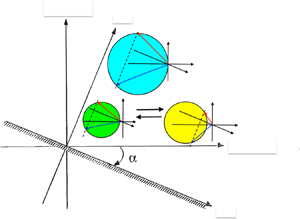
Consider a $\beta$-plane with a coordinate system $(x,y,z)$ in which $x$ is parallel and $y$ is perpendicular to the coast or channel and $z$ is vertically upwards (figure 1). For the coast, there is a vertical wall at the plane $y = 0$ and for the channel, of width $W$, there is another vertical wall at the plane $y = W$. The origin is somewhere in a mid-latitude region. The governing equation is the QGPVE, which in this coordinate system reads

(2.1)\begin{equation} \left\{ \left[ \partial_{t} + J(\psi,\cdot) \right] \left[ \nabla^2 + \partial_{z} (\varGamma^2 \partial_{z}) \right] + \beta (\cos \alpha \, \partial_{x} + \sin \alpha \, \partial_{y}) \right\} \psi = 0 , \end{equation}

where $\alpha$ is the angle that the coast makes with the circles of latitude (positive clockwise), $J(a,b) \equiv \partial _{x} a\,\partial _{y} b - \partial _{x} b \, \partial _{y} a$ the Jacobian operator, $\nabla ^2 = \partial _{x} \partial _{x} + \partial _{y} \partial _{y}$, $t$ is the time, $\psi$ is the quasi-geostrophic streamfunction, $\beta$ is the northward gradient of the planetary vorticity and $\varGamma ^2(z) \equiv f_0^2/N^2(z)$, where $f_0$ is the Coriolis parameter and $N(z)$ is the Brunt–Väisälä frequency.

Figure 1. Coordinate system. The rotated coordinate system has $x$ parallel and $y$ perpendicular to the coast; $\alpha$ is measured positive clockwise. For the channel of width $W$, there is another coast at $y = W$.

For the coast, the kinematic boundary condition of no normal flow is $\partial _{x} \psi = 0$ at $y = 0$; and for the channel it is $\partial _{x} \psi = 0$ at $y = 0, W$. Since the domain is partially open, an explicit mass conservation constraint or time-independent circulation is not required (Pinardi & Milliff Reference Pinardi and Milliff1989). Besides, for the type of solutions we will be considering (a sum of Rossby modes), the coasts’ condition implies $\psi = 0$ there. The boundary conditions in $z$ are those for a flat bottom and a rigid lid, i.e. $[ \partial _{t} + J(\psi ,\cdot ) ] \partial _{z} \psi = 0$ at $z = -H, 0$, where $H$ is the constant water depth. These conditions will be automatically satisfied, since the $z$-dependence of the Rossby modes is given in terms of eigenfunctions $\varphi _{n_j}(z)$ of the familiar vertical Sturm–Liouville problem (Pedlosky Reference Pedlosky2013).

Without going into the details, the general approach to studying the weakly nonlinear interaction between two Rossby modes of a coast or a channel is as follows. One first obtains the non-dimensional version of the QGPVE (2.1) by choosing suitable scaling parameters. There appears a parameter $\varepsilon = U \beta ^{-1} L^{-2}$ multiplying the nonlinear terms, which is the $\beta$-Rossby number, where $U$ and $L$ are the scales for the horizontal velocity and length. One then assumes $\varepsilon \ll 1$ and writes the solution as a perturbation expansion $\psi = \psi ^{(0)} + \varepsilon \psi ^{(1)} + \ldots\ $.

Therefore, mathematically, the problem is to solve the (dimensional) equation

(2.2)\begin{equation} \mathcal{L}\psi ^{(1)} ={-}J\left( \psi ^{(0)},\nabla ^{2}\psi ^{(0)}+\partial _{z}\left[ \varGamma ^{2}\partial _{z}\psi ^{(0)}\right] \right) , \end{equation}

where

(2.3)\begin{equation} \mathcal{L}\equiv \partial _{t}\left( \nabla ^{2}+\partial _{z}\left[ \varGamma ^{2}\partial _{z}\right] \right) +\beta \left( \cos \alpha \partial _{x}+\sin \alpha \partial _{y}\right) , \end{equation}

and $\psi ^{(0)}$ is the leading-order solution, chosen to be the superposition of any two free Rossby modes for a straight coast or a channel

(2.4)\begin{align} \psi ^{(0)} &=\psi _{1}^{(0)}+\psi _{2}^{(0)} \nonumber\\ &=\sum_{j=1}^{2}A_{j}\varphi_{n_j}(z)\left[ \cos \left( \theta_{1j}\right) - \cos \left( \theta _{2j}\right) \right] \nonumber\\ &\equiv \psi _{11}^{(0)}-\psi _{21}^{(0)}+\psi _{12}^{(0)}-\psi _{22}^{(0)}. \end{align}

In the last expression, we have defined the streamfunctions of the four RWs, two of each mode, given by

(2.5)\begin{align} \psi _{ij}^{(0)} &=A_{j}\varphi _{n_{j}}(z) \cos \left( \theta_{ij} \right) \nonumber\\ &\equiv A_{j}\varphi _{n_{j}}(z) \cos \left( k_{j}x+l_{ij}y-\omega _{j}t + \vartheta_j \right) ,\quad j=1,2;\ i=1,2 , \end{align}

where for the $j$th mode, $A_j$ and $\vartheta _j$ are the (real) amplitude and phase, respectively, $k_j$ is the wavenumber parallel to the coast or channel and $\omega _j$ is the frequency; and $l_{ij}$ is the wavenumber perpendicular to the coast or channel of the $i$th RW of the $j$th mode.

Our interest is in studying the possibility of having resonant interactions between three Rossby modes on a coast or channel of arbitrary orientation. Therefore, we ask whether the forcing of (2.2), i.e. its right-hand side, with $\psi ^{(0)}$ given by (2.4), could produce a third mode, namely,

(2.6)\begin{equation} \psi_3^{(1)} = A_{3}\varphi_{n_3}(z)\left[ \cos \left( \theta_{13} \right) - \cos \left( \theta _{23}\right) \right] , \end{equation}

which is a solution (or free Rossby mode) in the geometry considered.

Of course, each Rossby mode, including the forced mode, must satisfy the relationships

(2.7)\begin{gather} 2\omega _{j}l_{0j}+\beta \sin \alpha =0, \end{gather}

(2.8)\begin{gather}\omega _{j}\left( k_{j}^{2}+l_{0j}^{2}+\varDelta_{j}^{2}+\hat{a} _{n_{j}}^{{-}2}\right) +\beta \left( k_{j}\cos \alpha +l_{0j}\sin \alpha \right) =0, \end{gather}

or, in compact form, the relation

(2.9)\begin{equation} \varDelta_{j}^{2}=\,f_{n_{j}}\left( k_{j},\omega _{j}\right) \equiv \frac{\beta ^{2}}{4\omega _{j}^{2}}-\hat{a}_{n_{j}}^{{-}2}-\left( k_{j}+\frac{\beta \cos \alpha }{2\omega _{j}}\right) ^{2}, \end{equation}

for $j=1,2,3$, where $\hat {a}_{n_j}$ is the baroclinic Rossby radius of the $n_j$ vertical mode. We know that the component of the wavenumber vector perpendicular to the wall(s) that form each of the modes, is determined by

(2.10)\begin{equation} l_{1j,2j} = l_{0j} \pm \varDelta_{j} , \quad j=1,2,3, \end{equation}

with $l_{0j}$ given by (2.7). In what follows, we will call $l_{1j}$ the incident wave and $l_{2j}$ the reflected wave of the $j$th mode (this holds true for all orientations of the straight coast if $\varDelta _j > 0$ – see Graef & Magaard Reference Graef and Magaard1994). Obviously, in the case of a channel, the terms incident and reflected make no sense; however, this denomination helps us not to introduce new terms and clearly does not lead to confusion.

Finally, we note that, upon using some trigonometric identities, the streamfunction of the $j$th mode (see (2.4)) can be written as

(2.11)\begin{equation} \psi_j^{(0)} ={-} 2 A_j \varphi_{n_j}(z) \, \sin \left( k_j x + l_{0j} y -\omega_j t + \vartheta_j \right) \, \sin(\varDelta_j y) , \end{equation}

i.e. the mode is ‘sort of’ a standing wave in the direction perpendicular to the coast or channel ($y$-direction), but still propagating in the $(k_j,l_{0j})$ horizontal direction. Also, for a channel, it is $\varDelta _j = m_j {\rm \pi}/W$, where $m_j = 1,2,3, \ldots$ and it is easy to see from (2.11) that $\psi _j^{(0)}$ satisfies the boundary condition at $y = 0$ for the coast, or at $y = 0, W$ for the channel.

3. Which forcings could produce a third mode?

We know that the nonlinear interaction between two waves produces forcing terms with the sum and difference of the wave phases, and that to form a mode we need to have two RWs, of equal wavenumber in the $x$-direction, with the same frequency and identical vertical structures. We will now see which of the forcings (produced by the interaction of the waves of the ‘initial’ or primary modes) we should consider to form a third Rossby mode. For both problems (coast and channel), we will point out the difference between the zonal and non-zonal orientations.

3.1. Forcings produced by the self-interaction of one or both modes

This case only applies when the geometries are not zonally oriented. First, we analyse the forcings produced by the self-interaction of both primary modes. As the forced mode must be the sum of two RWs of equal frequency and equal wavenumber component in the $x$-direction, we obtain that $\omega _3 = 2 \omega _1 = 2 \omega _2$, and $k_3 = 2k_1 = 2k_2$. Therefore, the modes ‘initially’ considered or primary modes are equal, and this has already been studied by Graef (Reference Graef1993) for the straight coast and by García & Graef (Reference García and Graef1998) for the channel.

Now we analyse the case in which one of the forcings is produced by the self-interaction of one mode, and the other forcing is produced by the interaction of one of the RWs of one mode with one of the RWs of the other mode. In such a situation we get

(3.1)\begin{equation} \left. \begin{gathered} \omega _{3} =2\omega _{1}=\omega _{1}\pm \omega _{2} \quad \Longrightarrow \quad \omega_{2}={\pm} \omega _{1} ,\\ k_{3} =2k_{1}=k_{1}\pm k_{2} \quad \Longrightarrow \quad k_{2}={\pm} k_{1}, \end{gathered} \right\} \end{equation}

where the $\pm$ sign indicates the sum or difference of the wave phases in the forcing terms produced by the interacting waves. Again, the primary modes match, and we are in the previous case. Another possibility from (3.1) arises if we exchange $\omega _1$ and $\omega _2$, so that we consider the self-interaction of mode 2. In such a case

(3.2)\begin{equation} \left. \begin{gathered} \omega_{3} =2\omega_{2}=\omega _{1}\pm \omega _{2} \quad \Longrightarrow \quad \omega_{1} = 3\omega_{2} , \\ k_{3} =2k_{2}=k_{1}\pm k_{2} \quad \Longrightarrow \quad k_{1} = 3 k_{2}, \end{gathered} \right\} \end{equation}

where we chose the waves’ phase difference, otherwise we are in the case in which the primary modes match. Let us call $\omega _2 = \omega$, then $\omega _1 = 3 \omega$ and $\omega _3 = 2 \omega$. Then the wavenumbers perpendicular to the coast or channel of mode 3 are

(3.3)\begin{equation} \left. \begin{gathered} l_{13} =l_{12} + l_{22} = 2 l_{02} \quad (\text{self-interaction of mode 2}), \\ l_{23} =l_{11} - l_{12} . \end{gathered} \right\} \end{equation}

If it is a mode, necessarily $l_{13} + l_{23} = 2 l_{03} = -\beta \sin \alpha /(2 \omega ) = l_{02}$, since $\omega _3 = 2 \omega$ (in fact, from (2.7), it follows that $3 l_{01} = l_{02} = 2 l_{03}$). Thus, $l_{23} = - l_{02}$, which in combination with the second equation of (3.3) yields $l_{01} = \varDelta _2 - \varDelta _1$, upon using (2.10). Also $l_{13} - l_{23} = 2 \varDelta _3 = 3 l_{02}$. Thus, between the variables $\varDelta _j$, only one is independent, say $\varDelta _2$. Therefore, for this particular case in which the frequencies are multiples of $\omega$, we have three equations, one for each mode, i.e. (2.9) for $j=1,2,3$, and three unknowns: $\omega$, $k$ and $\varDelta _2$. If there is a solution for the coast, it is unique (there are no degrees of freedom). For the channel, since $\varDelta _j = m_j {\rm \pi}/W$ must be prescribed, there are two unknowns, the system is incompatible, and there are no solutions. We will not consider this particular case in any further analysis in what follows in this paper. Note, however, that only three RWs participate in exciting, in principle, a third mode.

Thus, it follows from the above considerations that: for a channel, a third Rossby mode can never be excited if we consider the forcing produced by the self-interaction of any one of the Rossby modes.

3.2. Forcings produced by the interaction of the four RWs

Let us take, without loss of generality, the forcing produced by the interaction of the incident waves of each mode and the forcing produced by the interaction of the reflected waves of each one. Thus, the four waves, two of each mode, participate in the formation of a third mode, whose wave parameters are given by

(3.4)\begin{equation} \left. \begin{gathered} \omega _{3} =\omega _{1}\pm \omega _{2}, \\ k_{3} =k_{1}\pm k_{2}, \\ l_{13} =l_{11}\pm l_{12}, \\ l_{23} =l_{21}\pm l_{22}. \end{gathered} \right\} \end{equation}

The sum of the last two relations of (3.4) establishes that

(3.5)\begin{equation} l_{03}=l_{01}\pm l_{02}, \end{equation}

which is trivially satisfied if the coast or channel is zonal ($\sin \alpha = 0$). On the other hand, if the coast or channel is not zonally oriented, (3.5) yields, upon substituting (2.7)

(3.6)\begin{equation} \left( \omega _{2}\pm \omega _{1}\right) \left( \omega _{1}\pm \omega _{2}\right) -\omega _{1}\omega _{2} = 0, \end{equation}

which is satisfied only if

(3.7)\begin{equation} \omega_{2} = \tfrac{1}{2} \left({-}1\pm \textrm{i}\sqrt{3}\right) \omega _{1}, \end{equation}

if the sum of the phases is considered; or

(3.8)\begin{equation} \omega_{2} = \tfrac{1}{2} \left( 1\pm \textrm{i}\sqrt{3}\right) \omega _{1}, \end{equation}

if the difference of the phases is considered (in these solutions for $\omega _2$, the $\pm$ refers obviously to the two roots). From (3.7) or (3.8), which are the product of the sum or difference of the wave phases, one can see that if the frequency of one of the modes is real (as it must be), the frequency of the other is complex, which does not constitute a free Rossby mode. The case $\omega _1 = \omega _2 = 0$ is not possible because we are in the non-zonal orientation $\sin \alpha \neq 0$, in which stationary currents cannot be solutions of the QGPVE without an external forcing.

Therefore, for a non-zonally oriented coast or channel, the forcings produced by the interaction between the four RWs of the primary modes can never excite a third mode.

3.2.1. Zonal case

We already saw that the sum $l_{13} + l_{23}$ from (3.4) is trivially satisfied if the coast or channel is zonal. However, the difference $l_{13} - l_{23}$ yields $\varDelta _3 = \varDelta _1 \pm \varDelta _2$, which means that a new horizontal structure is produced by the resonant interactions, i.e. there is ‘barotropic transfer’. Therefore, for the zonal case, the kinematic conditions that must be satisfied for resonance to occur between three Rossby modes are

(3.9)\begin{equation} \left. \begin{gathered} \omega_{j}\left( k_{j}^{2}+\varDelta_{j}^{2}+\hat{a}_{n_{j}}^{{-}2}\right) +\beta k_{j} = 0 ,\quad j=1,2,3, \\ \omega_{3} = \omega_{1} \pm \omega _{2}, \\ k_{3} = k_{1} \pm k_{2}, \\ \varDelta_{3} = \varDelta_{1} \pm \varDelta_{2}. \end{gathered} \right\} \end{equation}

These conditions are identical to those posed by Longuet-Higgins & Gill (Reference Longuet-Higgins and Gill1967) in their study on resonant interactions between barotropic planetary waves. However, our case is a generalization of that work, since here we consider a continuously stratified ocean and the coupling between the vertical structure of the modes. Incidentally, we should mention the work by Vanneste (Reference Vanneste1995), who treated the nonlinear interaction among normal modes in a multilayer QG (zonal) channel.

In general, there are six equations and twelve variables: $\omega _j$, $k_j$, $\varDelta _j$ and $n_j$. The last three (the $n_j$) must be specified, and therefore we end up with a system with three degrees of freedom. It is convenient to note that the variables that define the third Rossby mode, except for its vertical structure $n_3$, may not be taken into account to determine the degrees of freedom of the resonance conditions. In such a case the last three relations of (3.9) are eliminated, to obtain the system

(3.10)\begin{equation} \left. \begin{gathered} \omega _{1}\left( k_{1}^{2}+\varDelta _{1}^{2}+a_{n_{1}}^{{-}2}\right) +\beta k_{1} = 0, \\ \omega _{2}\left( k_{2}^{2}+\varDelta _{2}^{2}+a_{n_{2}}^{{-}2}\right) +\beta k_{2} = 0, \\ \left( \omega _{1}\pm \omega _{2}\right) \left[ \left( k_{1}\pm k_{2}\right) ^{2}+\left( \varDelta _{1}\pm \varDelta _{2}\right) ^{2}+a_{n_{3}}^{{-}2} \right] +\beta \left( k_{1}\pm k_{2}\right) = 0 . \end{gathered} \right\} \end{equation}

Now we have three equations and nine unknowns, but when we specify the discrete variables $n_j$, we get a system with three degrees of freedom.

For a channel of constant width $W$, however, the variables $\varDelta _1 = m_1 {\rm \pi}/W$ and $\varDelta _2 = m_2 {\rm \pi}/W$ need to be specified. Thus, the system (3.10) has only one degree of freedom. This case is similar to the study of Plumb (Reference Plumb1977).

Finally, we note the following fact. In the zonal case, and this is true for the coast or channel, if the nonlinear interaction between one RW of mode 1 and one RW of mode 2 excites a free RW, i.e. if for example $\{\psi _{11}^{(0)}, \psi _{12}^{(0)},\psi _{13}^{(0)}\}$ form a resonant triad, then it follows that the interaction between the other RW of mode 1 and the other RW of mode 2, also forces another free RW, i.e. $\{\psi _{21}^{(0)}, \psi _{22}^{(0)},\psi _{23}^{(0)}\}$ also form a resonant triad; and further, these two new waves form a third mode. In other words, the forcing of a third mode occurs automatically. This does not happen in the non-zonal case. Therefore, the zonal orientation is less restrictive in terms of finding resonance among modes.

3.3. Forcings produced by the interaction of three RWs

Let us now consider the forcing that is produced by the interaction of one of the RWs of one mode with the two RWs of the other mode. In that case, without loss of generality, we have

(3.11)\begin{equation} \left. \begin{gathered} \omega _{3} =\omega _{1}\pm \omega _{2}, \\ k_{3} =k_{1}\pm k_{2}, \\ l_{13} =l_{11}\pm l_{12}, \\ l_{23} =l_{11}\pm l_{22}. \end{gathered} \right\} \end{equation}

The sum of the last two relations of (3.11) yields

(3.12)\begin{align} l_{03} &=l_{11}\pm l_{02}, \end{align}

(3.13)\begin{align} &=l_{01}+\varDelta _{1}\pm l_{02} , \end{align}

which, in terms of the frequencies, i.e. using (2.7), is

(3.14)\begin{equation} \varDelta _{1}= \left( \frac{\pm \omega _{3}^{2}-\omega _{1}\omega _{2}}{2\omega _{1}\omega _{2}\omega _{3}} \right) \, \beta \sin \alpha . \end{equation}

Equation (3.14) that relates $\omega _1$, $\omega _2$ and $\varDelta _1$, is additional to the three equations (one for each Rossby mode), and distinguishes the non-zonal case from the zonal case. It also reduces the degrees of freedom.

If the coast or channel is zonally oriented, from (3.14) it follows that $\varDelta _1 = 0$, but this implies that $l_{11} = l_{21} = 0$, i.e. only one RW with the group velocity parallel to the coast and whose solution is ${\sim }y \cos (k x - \omega t)$, physically there is no reflection; and for the channel this means that there is no mode 1 (see Graef Reference Graef2017). Thus, the interaction of three RWs cannot produce a third mode in the zonal case.

On the other hand, the difference of the last two relations of (3.11) yields

(3.15)\begin{equation} l_{13} - l_{23} ={\pm} \left(l_{12} - l_{22} \right) \quad \Longrightarrow \quad \varDelta_3 ={\pm} \varDelta_2 . \end{equation}

Therefore, the horizontal structure of the ‘standing’ part of the forced mode is identical to that of the mode whose two RWs participate in the interaction (mode 2 in this case). Resonant interactions do not produce new horizontal structure in the non-zonal case.

From the results obtained above it follows that:

1. (i) If the coast or channel is zonally oriented, we need the participation or interaction of the four RWs, two of each mode, to excite a third Rossby mode that can resonantly interact with the modes that originate it.

2. (ii) If the coast or channel is not zonally oriented, only three waves (of the four RWs) can participate in exciting, in principle, a third mode that can resonantly interact with the modes that originate it.

3. (iii) Only in the zonal case is a new horizontal structure created, i.e. there is ‘barotropic transfer’.

In the non-zonal case, the kinematic conditions for resonance to occur between three Rossby modes can be written as

(3.16)\begin{gather} \left( k_{1}+\frac{\beta \cos \alpha }{2\omega _{1}}\right) ^{2}+\varDelta _{1}^{2}-\frac{\beta ^{2}}{4\omega _{1}^{2}}+\hat{a}_{n_{1}}^{{-}2} =0, \end{gather}

(3.17)\begin{gather}\left( k_{2}+\frac{\beta \cos \alpha }{2\omega _{2}}\right) ^{2}+\varDelta _{2}^{2}-\frac{\beta ^{2}}{4\omega _{2}^{2}}+\hat{a}_{n_{2}}^{{-}2} =0, \end{gather}

(3.18)\begin{gather}\left[ \left( k_{1}\pm k_{2}\right) +\frac{\beta \cos \alpha }{2\left( \omega _{1}\pm \omega _{2}\right) }\right] ^{2}+\varDelta _{2}^{2}-\frac{\beta ^{2}}{4\left( \omega _{1}\pm \omega _{2}\right) ^{2}}+a_{n_{3}}^{{-}2} =0, \end{gather}

(3.19)\begin{gather}\varDelta _{1}^{2}-\frac{\left[ \left( \omega _{1}\pm \omega _{2}\right) ^{2}\mp \omega _{1}\omega _{2}\right]^2}{4\omega _{1}^{2}\omega _{2}^{2}\left( \omega _{1}\pm \omega _{2}\right) ^{2}} \, \beta ^{2}\sin ^{2}\alpha =0 . \end{gather}

Thus, unlike the zonal case, in the non-zonal case we have a system with nine unknowns: $k_1$, $k_2$, $\varDelta _1$, $\varDelta _2$, $n_1$, $n_2$, $n_3$, $\omega _1$ and $\omega _2$, but four equations. Once we specify the $n_j$, we have a system with two degrees of freedom. For a channel of width $W$, where $\varDelta _1 = m_1 {\rm \pi}/W$ and $\varDelta _2 = m_2 {\rm \pi}/W$ need to be specified, the system (3.16)–(3.19) is compatible and determined; that is to say, there are no degrees of freedom. If a solution exists, it is unique.

The solutions of (3.16)–(3.19), for both geometries, will be discussed in the next two sections.

4. Resonant interactions of Rossby modes in a straight coast

We will only treat the non-zonal orientation since, as discussed before, the case of a zonal coast is identical to the work done by Longuet-Higgins & Gill (Reference Longuet-Higgins and Gill1967). The resonant conditions (3.16)–(3.19) can be rewritten as

(4.1)\begin{gather} \varDelta _{1}^{2} =\,f_{n_{1}}\left( k_{1},\omega _{1}\right), \end{gather}

(4.2)\begin{gather}\varDelta _{2}^{2} =\,f_{n_{2}}\left( k_{2},\omega _{2}\right), \end{gather}

(4.3)\begin{gather}\varDelta _{2}^{2} =\,f_{n_{3}}\left( k_{1}\pm k_{2},\omega _{1}\pm \omega _{2}\right), \end{gather}

(4.4)\begin{gather}\varDelta _{1}^{2} =g\left( \omega _{1},\omega _{2}\right) , \end{gather}

where

(4.5)\begin{equation} f_{n}\left( k,\omega \right) \equiv \frac{\beta ^{2}}{4\omega ^{2}}-\hat{a}_{n}^{{-}2}- \left( k+\frac{\beta \cos \alpha }{2\omega }\right) ^{2} \end{equation}

and

(4.6)\begin{equation} g\left( \omega _{1},\omega _{2}\right) \equiv \frac{\left[ \left( \omega _{1}\pm \omega _{2}\right) ^{2}\mp \omega _{1}\omega _{2}\right] ^{2}} {4\omega _{1}^{2}\omega _{2}^{2}\left( \omega _{1}\pm \omega _{2}\right)^{2}} \, \beta ^{2}\sin ^{2}\alpha . \end{equation}

Equating (4.1) and (4.4) to eliminate $\varDelta _1$, we get a quadratic in $k_1$

(4.7) \begin{align} & 4\omega _{1}^{2}\omega _{2}^{2}\omega _{3}^{2}k_{1}^{2}+4\omega _{1}\omega _{2}^{2}\omega _{3}^{2}\beta \left( \cos \alpha \right) k_{1}+\omega _{3}^{4}\beta ^{2}\sin ^{2}\alpha + \omega _{2}\omega _{3}^{2} \nonumber\\ &\quad \times \left[ 4\omega _{1}^{2}\omega _{2}\hat{a}_{n_{1}}^{{-}2}-\left( \omega _{2}\pm 2\omega _{1}\right) \beta ^{2}\sin^{2}\alpha \right] + \omega _{1}^{2}\omega _{2}^{2}\beta^{2} \sin ^{2}\alpha = 0 , \end{align}

where the variable $\omega _3$ has been left in (4.7) for simplicity. Solving for $k_1$, after substituting $\omega _3$ by $\omega _1 \pm \omega _2$, and some algebra and simplifications, we obtain

(4.8)\begin{equation} k_1^{(1,2)} ={-} \frac{\beta \cos \alpha}{2 \omega_1} \pm \frac{1}{2} \left[ \beta^2 \left( \frac{\cos^2 \alpha} {\omega_1^2} - \frac{\sin^2 \alpha}{\omega_2^2} \right) - 4\hat{a}_{n_1}^{{-}2} - \frac{\beta^2 \sin^2 \alpha}{(\omega_1 \pm \omega_2)^2} \right]^{1/2} . \end{equation}

Thus, there are two roots or solutions: $k_1^{(1)}$ and $k_1^{(2)}$, corresponding to the $+$ and $-$ in front of $\tfrac {1}{2} [\ldots ]^{1/2}$, respectively, for the phase sum ($\omega _1 + \omega _2)$, or for the phase difference ($\omega _1 - \omega _2)$. We could not find a condition that only involves the coast orientation $\alpha$ to have $k_1^{(1,2)}$ real. However, it is easy to see that there are no real solutions for a meridional coast ($\alpha = {\rm \pi}/2$). The real solutions are restricted to more zonally oriented coasts. We need real wavenumbers parallel to the coast, otherwise, the solution blows up as $x \longrightarrow \pm \infty$. A necessary condition to have $k_1^{(1,2)}$ real is

(4.9)\begin{equation} |\sin \alpha| \leq \left[ \frac{(1 \pm r)^2 \, r^2} {(1+r^2)(1\pm r)^2 + r^2} \right]^{1/2}, \end{equation}

where $r = \omega _2/\omega _1 = T_1/T_2$ and $T_1 = 2 {\rm \pi}/\omega _1$, $T_2 = 2 {\rm \pi}/\omega _2$ are the primary modes’ periods. This condition is in terms of $|\sin \alpha |$, as in previous works (Graef Reference Graef1993; García & Graef Reference García and Graef1998), and one can easily see special cases. For example, if $r=1$ (initial modes have equal frequency) it reduces to $|\sin \alpha | \leq 2/3$ (see (4.11) below) and if $r=2$ (i.e. $\omega _2=2\omega _1$) $|\sin \alpha | \leq 6/7$.

Figure 2 shows the function $X_{\pm }(r,\alpha ) = |\sin \alpha |^2 - (1 \pm r)^2 \, r^2/[(1+r^2)(1\pm r)^2 + r^2]$ in which the yellow regions are prohibited ($X_{\pm } > 0$); note the region around a meridional coast ($\alpha = 90^{\circ }$). If $k_1^{(1,2)}$ are real then $r$ and $\alpha$ must be in the green and blue regions where $X_{\pm } < 0$. Large values of $r$ or $T_1 \gg T_2$ favour real solutions for more meridionally oriented coasts ($\alpha \in (70,85)$ or $\alpha \in (95,110)\, ^{\circ }$).

Figure 2. The function $X_{\pm }(r,\alpha )$, where $r = \omega _2/\omega _1$ and $\alpha$ is the angle between the eastern direction and the coast (in degrees). If $k_1^{(1,2)}$ are real, then $r$ and $\alpha$ must be in the green and blue regions $X_{\pm } < 0$. Yellow regions have $X_{\pm } > 0$, for which $k_1^{(1,2)}$ are complex: (a) is $X_+$; (b) is $X_-$.

To complete the story, however, we still need to calculate the wavenumber $k_2$ of the second mode. This is accomplished by equating (4.2) and (4.3) to eliminate $\varDelta _2$, but this time the term $k_2^2$ drops out, and we get a linear equation in $k_2$

(4.10) \begin{align} \left( \pm2k_1 \pm \frac{\beta \cos \alpha}{\omega_1 \pm \omega_2} - \frac{\beta \cos \alpha}{\omega_2} \right) k_2 &= \frac{\beta^2 \sin^2 \alpha}{4} \left[ \frac{1}{(\omega_1 \pm \omega_2)^2} - \frac{1}{\omega_2^2} \right] \nonumber\\ &\quad + \hat{a}_{n_2}^{{-}2} - \hat{a}_{n_3}^{{-}2} - k_1^2 - \frac{\beta \cos \alpha}{\omega_1 \pm \omega_2} k_1 \end{align}

From (4.10) we can easily solve for $k_2$ and substitute the roots $k_1^{(1,2)}$ to obtain $k_2^{(1,2)}$ for either the sum or phase difference. It is worth remarking that both (4.8) and (4.10) are necessary conditions to have solutions of the system (4.1)–(4.4). That is, with the roots $k_1^{(1,2)}$ we have to go back to (4.1) to calculate $\varDelta _1^2$; similarly, with $k_2^{(1,2)}$, we go back to (4.2) or (4.3) to calculate $\varDelta _2^2$. Thus, the whole solution is obtained.

In the previous section, we showed that we have two degrees of freedom in this problem. Given the frequencies of the primary modes $\omega _1$ and $\omega _2$, we can get the wavenumbers along the coast of the first mode $k_1^{(1,2)}$ and second mode $k_2^{(1,2)}$, for either the sum or phase difference of the interacting RWs. Thus, for each $\omega _1$ and $\omega _2$, there are two solutions $k_{1p}^{(1,2)}$ for the phase sum and two solutions $k_{1m}^{(1,2)}$ for the phase difference.

In figure 3 we show the real solutions $k_{1p,m}^{(1,2)}$ as a function of the mode periods $T_1$ and $T_2$ for values appropriate for the Hawaiian Ridge: reference latitude $\phi _0 = 21^{\circ }$ and $\alpha = 25^{\circ }$; we choose a first baroclinic mode $n_1=1$ for Rossby mode 1. Note that the ($T_1,T_2$) space of real solutions is more restrictive ($T_1 > T_2$) for the phase difference than for the phase sum. Due to (4.10), if $k_1$ is complex, then $k_2$ is complex. Thus, the white regions of figure 3 will be exactly the same for the wavenumber $k_2$ of the second mode.

Figure 3. The solutions for the wavenumbers $k_1^{(1,2)}$ from (4.8) as a function of the mode periods $T_1$ and $T_2$ in years. Panels (a,b) and (c,d) correspond to the phase sum and phase difference, respectively. Panels (a,c) and (b,d) show $k_1^{(1)}$ and $k_1^{(2)}$, respectively. The white regions yield complex solutions. Reference latitude $\phi _0 = 21^{\circ }$, $\alpha = 25^{\circ }$, which are values appropriate for the Hawaiian Ridge; $n_1 = 1$.

To give an idea of the RWs of each mode of the resonant triad, we calculate their wavelengths as a function of $T_1$ and $T_2$ for values of the Hawaiian Ridge and vertical mode numbers $n_1 = 1$, $n_2 = 1$ and $n_3 = 2$ (see figures 4–7). A few notes about these four figures are in order. First, the allowed ($T_1,T_2$) space is reduced further for the wavelengths (as compared with the one for $k_1$ of figure 3) because we only permit solutions that yield real wavenumber components perpendicular to the coast (otherwise the solution blows up as $y \longrightarrow \infty$). That is, the fact that the $k$ values are real does not guarantee that the $l$ values are real, so when calculating the $l$ values, we must require $\varDelta ^2_2 > 0$ (see (2.9) and (2.10)); note that $\varDelta ^2_1 > 0$ by (4.4) and (4.6) and we have $\varDelta ^2_3 = \varDelta ^2_2$. Therefore, the approach to correctly understanding figures 4–7 is to choose the periods $(T_1, T_2)$ such that they fall on coloured regions in all 6 panels of each figure. Figures 4 and 5 show the wavelengths of the incident and reflected RWs of the three modes corresponding to the solutions $k_{1p}^{(1)}$ and $k_{1m}^{(1)}$, respectively. For the phase sum $\omega _1 + \omega _2$ (figure 4), the range of wavelengths for the first mode is $\lesssim 1000\ \textrm {km}$ for the incident RW (note the white wedge in modes 2 and 3) and $\lesssim 50$ for the reflected RW; for the second mode, the ranges are [100, 240] km and [20, 120] km, respectively; and for the third mode they are [100, 1400] km and $[\lesssim 50,200]\ \textrm {km}$, respectively. Note, however, that in general the space for the larger wavelengths is squeezed into a very small region. For the phase difference $\omega _1 - \omega _2$ (figure 5), the range of wavelengths is: $\lesssim 1000$ (note the small white wedge in modes 2 and 3 for very small $T_2$) and $[\lesssim 20,100]$; $[\lesssim 50,200]$ and [20, 140]; and $[\lesssim 100,2000]$ and $[\lesssim 20,120]$, for the incident and reflected and for modes 1, 2 and 3, respectively.

Figure 4. Wavelengths (in km) of the incident (a,c,e) and reflected (b,d,f) RWs of mode 1 (a,b), mode 2 (c,d) and mode 3 (e,f) corresponding to the solution $k_{1p}^{(1)}$ as a function of the mode periods $T_1$ and $T_2$ in years. Here, $\phi _0$ and $\alpha$ are appropriate for the Hawaiian Ridge and the vertical mode numbers are $n_1 = 1$, $n_2 = 1$, $n_3 = 2$.

Figure 5. As in figure 4, but for the solution $k_{1m}^{(1)}$.

Figures 6 and 7 show the wavelengths corresponding to the solutions $k_{1p}^{(2)}$ and $k_{1m}^{(2)}$, respectively. It is noteworthy that there is a dramatic reduction in the allowable ($T_1,T_2$) space for the solution superscript (2). This is mainly due to the fact, that for western coasts facing north, such as the Hawaiian Ridge, $\alpha \in (0, 90)$ degrees, $\cos \alpha > 0$ and $|k_1^{(2)}| > |k_1^{(1)}|$ (see (4.8)), so that in general $|k_2^{(2)}| > |k_2^{(1)}|$, making $\varDelta _2^2$ negative in a much larger region of the ($T_1,T_2$) space, thus reducing the space for real $l$ values. The real solutions for both $k$ and $l$ lie only within the very tiny region (resembling a slice of a pie), with $T_2 > T_1$ for solution $k_{1p}^{(2)}$ and $T_1 > T_2$ for $k_{1m}^{(2)}$. In both figures all the wavelengths are small: they range approximately between 20 and 200 km.

Figure 6. As in figure 4, but for the solution $k_{1p}^{(2)}$.

Figure 7. As in figure 4, but for the solution $k_{1m}^{(2)}$.

We produced figures 4–7 for a reference latitude $\phi _0 = 21^{\circ }$ and a coastal orientation $\alpha = 25^{\circ }$, which are values appropriate for the Hawaiian Ridge. We conclude that, in this case, the nonlinear interaction between two $n_1 = 1$ (first mode baroclinic) annual Rossby modes cannot excite a semi-annual $n_3 = 2$ Rossby mode. However, if instead we consider that the third or excited mode is barotropic with a free surface $n_3 = 0$ (depth $H = 4000\ \textrm {m}$), then those annual modes can resonantly interact to force a semi-annual mode (not shown here).

A general characteristic emerges by looking at different coastal orientations: the ($T_1,T_2$) space of real solutions is smaller for the phase difference than for the phase sum.

4.1. Modes of equal frequency

If the initial modes have equal frequencies, the number of variables is reduced by one (from 6 to 5), but the number of equations remains the same (four). There is still one degree of freedom, and we can exploit it to examine the possibilities to find resonance easily. This case is compelling because of its similarity to resonance occurring in the self-interaction of a Rossby mode (Graef Reference Graef1993).

For $\omega _1 = \omega _2 = \omega$, the solution (4.8), which only makes sense for the sum of the phases, is given by

(4.11)\begin{equation} k_1^{(1,2)} ={-} \frac{\beta \cos \alpha}{2 \omega} \pm \left[ \frac{\beta^2}{4 \omega^2} \left( 1 - \frac{9}{4} \sin^2 \alpha \right) - \hat{a}_{n_1}^{{-}2} \right]^{1/2} . \end{equation}

It is obvious that, to have $k_1^{(1,2)}$ real, it is necessary that $| \sin \alpha | \leq 2/3$. Again, the orientation of the coast or wall imposes a restriction for resonance to occur. We note that this value (of $|\sin \alpha |$) is twice that obtained by Graef (Reference Graef1993) when considering the self-interaction of a Rossby mode in a coast.

As can be observed from figure 4, there are solutions for $T_1 = T_2$ (i.e. $\omega _1 = \omega _2$) because a good part of the diagonal straight line lies within the coloured regions of all panels. But there are no solutions $\omega _1 = \omega _2$ for figure 6, since the diagonal is outside the coloured regions for modes 2 and 3.

5. Resonant interactions of Rossby modes in a channel

In a channel, we have already shown that there are no degrees of freedom. Once the 5 discrete variables (i.e. the three vertical mode numbers $n_j$, $j = 1,2,3$ and the two horizontal mode numbers $m_1$ and $m_2$) are specified, the kinematic conditions (3.16)–(3.19) or (4.1)–(4.4) form a closed system for the four unknowns: $\omega _1$, $\omega _2$, $k_1$ and $k_2$. If a solution exists, it is unique. The presence of a second boundary, as compared with the straight coast case (only one boundary), makes it a much more restrictive problem.

We tried but did not succeed in arriving at a single equation for any one of the four unknowns. However, using the solutions for the straight coast (4.8) and (4.10), we developed the following graphical method to seek for solutions:

1. (i) First, we give the mode number $m_1$ (i.e. $\varDelta _1$) and $\omega _1$. Then from (4.4) we solve for $\omega _2$, yielding

   (5.1)\begin{equation} \pm \omega_2^2 + \omega_1 \omega_2 \pm \omega_1 \left( \frac{1}{\omega_1} - \frac{2 \varDelta_1}{\beta \sin \alpha} \right)^{{-}1} = 0 , \end{equation}
   whose solution is
   (5.2)\begin{equation} \omega_2 ={\mp} \frac{\omega_1}{2} \pm \left[ \frac{\omega_1^2}{4} - \omega_1 \left( \frac{1}{\omega_1} - \frac{2 \varDelta_1}{\beta \sin \alpha} \right)^{{-}1} \right]^{1/2} ,\end{equation}
   in which, as usual, the $\mp$ in front of $\omega _1/2$ corresponds to the RWs’ phase sum (upper sign) and difference (lower sign), and the $\pm$ in front of the square root refers to the roots of $\omega _2$. A necessary and sufficient condition to have the frequency $\omega _2$ real is $2 \varDelta _1 \omega _1 > \beta \sin \alpha$, i.e. $T_1 < 4{\rm \pi} \varDelta _1/(\beta \sin \alpha )$. This condition (which could be derived by noting that, for a non-zonal channel, $\alpha \in (0,{\rm \pi} )$ covers all possible orientations so that $\sin \alpha > 0$) imposes a restriction on large periods for the first mode, but at the same time from the Rossby mode dispersion relation, (4.1) and (4.5), we need to have $\beta > 2 \omega _1 \varDelta _1$ or $T_1 > 4 {\rm \pi}\varDelta _1/\beta$. The conditions are opposed, showing us how restrictive it would be to find real solutions.

   Now, using (4.8), upon substituting (5.2), we draw the curves $k_1 = \mathcal {F} (\omega _1)$ (there will be four curves corresponding to the two roots $k_1^{(1,2)}$ and the two roots of (5.2) for the phase sum, and other four curves for the phase difference, eight curves total).

2. (ii) From (4.10) we have $k_2$ as a function of $k_1$. Draw the curve $k_2 = \mathcal {G}(k_1) = \mathcal {G}[\mathcal {F}(\omega _1)]$, i.e. $k_2$ as a function of $\omega _1$ only.

3. (iii) Now considering $k_2$ of step 2, for it to be a solution, must also satisfy (4.2) or (3.17), which is the equation for mode 2, quadratic in $k_2$. That is, given $m_2$ (i.e. $\varDelta _2$) and substituting $\omega _2$ from (5.2) of step 1 into (3.17), we could draw the curve $\,f_{n_2}(k_2,\omega _2) = \varDelta _2^2$ of this mode for each $\omega _1$.

4. (iv) The intersections of the curves of step 2 and step 3, if they exist, are the solutions for $k_2$ (it could be for more than one frequency $\omega _1$ if there is more than one intersection).

5. (v) The solutions for $k_1$ would correspond to the same abscissas $\omega _1$ at which the curves for $k_2$ intersect, but on the curve of step 1: $k_1 = \mathcal {F} (\omega _1)$.

In figures 8–10 we show an example of the graphical method just described, where we have chosen the period of the first mode $T_1$ as the independent variable instead of the frequency $\omega _1$. The chosen parameters are: $\phi _0 = 20^{\circ }$, $\alpha = 15^{\circ }$, channel width $W = 500\ \textrm {km}$, horizontal mode numbers $m_1 = 2$, $m_2 = 1$ (recall $m_3 = \pm m_2$) and vertical mode numbers $n_j = (0,0,0)$, i.e. a fully barotropic case with a free surface and a depth $H = 4000\ \textrm {m}$. Figure 8 shows solution (5.2) in terms of the periods, i.e. $T_2$ as a function of $T_1$. There are four curves, two in each panel, which correspond to the positive (blue) and negative (red) root of $\omega _2$ (or $T_2$). The upper (lower) panel refers to the RWs’ phase sum (difference). Note that, for the chosen parameters, $T_1$ cannot be larger than 0.9 years (recall the restriction $4 {\rm \pi}\varDelta _1/\beta < T_1 < 4{\rm \pi} \varDelta _1/(\beta \sin \alpha )$).

Figure 8. Periods $T_2$ of the second mode as a function of $T_1$ (years) from solution (5.2). Here, $\phi _0 = 20^{\circ }$, $\alpha = 15^{\circ }$, channel width $W = 500\ \textrm {km}$, horizontal mode number $m_1 = 2$ and vertical mode number $n_1 = 0$ (free surface, depth $H = 4000\ \textrm {m}$). Panels (a) and (b) show the phase sum and phase difference, respectively. Blue (red) curve refers to the positive (negative) root of $\omega _2$.

As regards to the solution of the resonance conditions, we observe that, for the phase sum (figure 9), there is only one solution, since the $k_2$-curves of steps 2 and 3 (blue and red, respectively) intersect in one panel only (a). Such a solution corresponds to the along channel wavenumbers $k_{1p1}^{(1)}$ of mode 1 and $k_{2p1}^{(1)}$ of mode 2, where the additional subscript (1 or 2) in $k_1$ and $k_2$ refers to the ($+$ or $-$) root of $\omega _2$ in (5.2).

Figure 9. Along channel wavenumbers ($\textrm {km}^{-1}$) $k_1$ (black) from step 1 and $k_2$ from steps 2 (blue) and 3 (red) of the graphical method (see text) as a function of $T_1$ (years). Panel (a) is $k_{1p1}^{(1)}$, where the additional subscript (1 or 2) in $k_1$ refers to the (+ or $-$) root of $\omega _2$ in (5.2), obtained from (4.8) and (5.2), and the corresponding $k_2$ from (4.10) (blue) and from (3.17) (red). Panel (b) is for $k_{1p1}^{(2)}$, (c) is for $k_{1p2}^{(1)}$ and (d) is for $k_{1p2}^{(2)}$. If the blue and red curves intersect (step 4), there is a real solution (as in a). Parameters as in figure 8, with $n_1 = 0$, $n_2 = 0$, $n_3 = 0$ (free surface, $H = 4000\ \textrm {m}$) and $m_1 = 2$, $m_2 = 1$.

On the other hand, for the phase difference (figure 10), there are three solutions, since the $k_2$-curves of steps 2 and 3 (blue and red, respectively) intersect in three panels (a,b,d), corresponding to solutions $(k_{1m1}^{(1)},k_{2m1}^{(1)})$, $(k_{1m1}^{(2)},k_{2m1}^{(2)})$ and $(k_{1m2}^{(2)},k_{2m2}^{(2)})$, respectively. However, the solutions of (b,d) represent the same Rossby modes (same mode parameters), but with mode 2 in one panel being mode 3 in the other panel, and vice versa. This can be seen by realizing that the solutions of these panels have identical $T_1$ (the blue and red curves intersect at the same abscissa) and identical $k_1$, so both solutions have equal first mode parameters. Also, the solution of (b) $(k_{1m1}^{(2)},k_{2m1}^{(2)})$ has $m_2 = 1$, $k_2 \approx -0.02\ \textrm {km}^{-1}$ from the graph, $m_3 = - 1$ (recall $\varDelta _3 = -\varDelta _2$ for the phase difference) and $k_3 = k_1 - k_2 \approx 0$; whereas the solution of (d) has $m_2 = -1$, $k_2 \approx 0$, $m_3 = 1$ and $k_3 = k_1 - k_2 \approx -0.02 \ \textrm {km}^{-1}$. Thus, mode 2 of (b) is mode 3 of (d) and vice versa; they are symmetric solutions with respect to modes 2 and 3.

Figure 10. As in figure 9, but for the phase difference, i.e. $k_{1m1}^{(1)}$ and $k_{1m1}^{(2)}$ for (a,b), respectively, and $k_{1m2}^{(1)}$ and $k_{1m2}^{(2)}$ for (c,d), respectively. Note that the blue and red curves intersect in (a,b,d), so there are real solutions.

Curiously enough, the only solution of the phase sum (figure 9a) and the solution of the phase difference corresponding to the figure 10(a), also represent the same Rossby modes, but with the parameters of mode 2 in one panel (or solution) being equal to minus the parameters of mode 3 in the other panel, and vice versa. We call these anti-symmetric solutions concerning modes 2 and 3. To explain, one solution is the phase sum (subscript $p$) and the other is the phase difference (subscript $m$), thus we have $k_{2p} = - k_{3m}$, $\omega _{2p} = - \omega _{3m}$ and $l_{12,22} = -l_{13,23}$. Now, if one computes the eastward phase speed $C_E = \omega /k_E$ of the RWs of each mode (2 and 3), where $k_E = k \cos \alpha + l \sin \alpha$ is the eastward wavenumber, the result is that the $C_E$ of mode 2 of the solution $p$ are equal to the $C_E$ of mode 3 of the solution $m$ and vice versa, and negative, i.e. all RWs have westward phase speed, as it should be. Thus, the anti-symmetric solutions with identical Rossby mode 1 and Rossby modes 2 and 3 exchanged have one of the modes (2 or 3) with the slowness circle on the $k_E < 0$ space (if the frequency is positive) and the other mode (3 or 2) on the $k_E > 0$ space (if the frequency is negative).

The graphical method of searching for the intersections of the $k_2$-curves of steps 2 and 3 (i.e. a change of sign of the difference between the $k_2$-curves) proved efficient in finding the solutions numerically. By choosing a sufficiently small time step of $10^{-5}$ year for the period $T_1$, we achieved numerical errors in the solutions for modes 1 and 2 of $O(10^{-18})$ and mode 3 of $O(10^{-10})$. The solution corresponding to figure 9(a) is: $(T_1, T_2, T_3) = (0.67, 0.52, 0.29)$ years, $(k_1, k_2, k_3) = (-0.0010,0.0002,-0.0008)\ \textrm {km}^{-1}$ and the wavelengths are: (1894, 286) km, (6254, 464) km and (2713, 604) km for modes 1, 2 and 3, respectively. And the solution corresponding to figure 10(d) is: $(T_1, T_2, T_3) = (0.26,-0.84,0.200)$ years, $(k_1, k_2, k_3) = (-0.0203,-0.0011,-0.0192)$ and the wavelengths are: (283, 242) km, (349, 1139) km and (296, 322) km for modes 1, 2 and 3, respectively.

If we just change the inclination of the channel to $\alpha = 5^{\circ }$, i.e. a more zonally oriented channel, and leave the rest of the input parameters used in figures 8–10 unchanged, we get intersections (solutions) in the same four panels. However, the periods are larger than the case $\alpha = 15^{\circ }$, although the wavelengths are similar.

As a possible oceanographic application, we searched for solutions in four channels with parameters resembling the Mozambique Channel ($\phi _0 = 19.5\,^{\circ }\textrm {S}$, $\alpha = 115^{\circ }$, $W = 750\ \textrm {km}$, $H = 3292\ \textrm {m}$), the Tasman Sea ($\phi _0 = 38^{\circ }$S, $\alpha = 110.5^{\circ }$, $W = 1750\ \textrm {km}$, $H = 2500\ \textrm {m}$), the Denmark Strait ($\phi _0 = 67\,^{\circ }\textrm {N}$, $\alpha = 146.5^{\circ }$, $W = 300\ \textrm {km}$, $H = 400\ \textrm {m}$) and the English Channel ($\phi _0 = 49\,^{\circ }\textrm {N}$, $\alpha = 157^{\circ }$, $W = 150\ \textrm {km}$, $H = 63\ \textrm {m}$) (Graef Reference Graef2017) and for the vertical and horizontal mode numbers used to produce figures 8–10, namely $n_j = (0,0,0)$ (all three modes barotropic, free surface) and $m_1 = 2$, $m_2 = 1$. There were no (real) solutions for the Mozambique Channel and the Tasman Sea because these channels are too inclined with respect to the eastern direction. However, we found solutions for the Denmark Strait and the English Channel. Again, there were four solutions (two and their mirror or symmetric or anti-symmetric solution with identical Rossby mode 1 and Rossby modes 2 and 3 exchanged) in each case, although the intersections of the curves (solutions) were for $k_{1p1}^{(2)}$ and its mirror or anti-symmetric $k_{1m1}^{(2)}$, and for $k_{1m1}^{(1)}$ and its mirror or symmetric $k_{1m2}^{(1)}$ (i.e. in different panels than in figures 9 and 10). The Rossby mode periods for the Denmark Strait are between 0.54 and 1.30 years, and the wavelengths between 167 and 2724 km. The second mode period of solution for $k_{1p1}^{(2)}$ is 1.00 year with wavelengths of 273 and 2724 km, which is also the period and wavelengths of the third mode of the solution $k_{1m1}^{(2)}$. Thus, if barotropic Rossby modes get excited in the Strait, out of all possible nonlinear interactions among them, the annual Rossby mode $m_2 = 1$ would have a larger amplitude since it is in resonance with two other modes of periods 0.56 and 1.24 years. The periods range between 0.79 and 2.47 years for the English Channel, and the wavelengths range between 79 and 1696 km.

After obtaining solutions for other parameters, in particular for various $\alpha$ values, i.e. for a diversity of channel orientations, the following picture emerges:

1. (a) There were always four solutions: one for the RWs’ phase sum and three for the RWs’ phase difference. The solutions came in pairs: a solution and its anti-symmetric or symmetric companion.

2. (b) The solution and its anti-symmetric or symmetric companion always correspond to the same root of $k_1$, either $k_1^{(1)}$ or $k_1^{(2)}$. They represent the same Rossby modes, but with modes 2 and 3 exchanged.

3. (c) The anti-symmetric solution arises from solutions corresponding to the RWs’ phase sum and phase difference, i.e. $k_{1p}$ and $k_{1m}$.

4. (d) The last two characteristics of the solutions are because $\varDelta _3 = \pm \varDelta _2$, which is a consequence of the non-zonal orientation and our choice that wave 1 of mode 1 (i.e. $l_{11}$) be the one that interacts with the two waves of mode 2 to produce a third channel mode. Had we chosen that the single wave is one of mode 2, then $\varDelta _3 = \pm \varDelta _1$, and the solution pair would come with modes 1 and 3 exchanged.

Therefore, we have found real solutions of the resonance conditions for three Rossby modes in a non-zonal channel, for both the RWs’ phase sum and difference. Because of the symmetric solutions, we could say that there are only two independent solutions for the waves’ phase difference. However, we must realize that, even though the symmetric solutions represent the same channel Rossby modes (with modes 2 and 3 exchanged), the amplitudes of modes 2 and 3 are different if we calculate the resonant solutions of the QGPVE at $O(\varepsilon )$.

Finally, we note that, in a non-zonal channel, the interaction of two Rossby modes of equal frequency can never excite a third Rossby mode. This is simply because, when two unknowns of the system (3.16)–(3.19) or (4.1)–(4.4) are made equal, the number of unknowns is reduced by one (from 4 to 3), but the number of equations remains the same (four). For instance, if $\omega _1 = \omega _2 = \omega$, the solution of (5.1) for $\omega \neq 0$ is $\omega = 3 \beta \sin \alpha /(4 \varDelta _1)$, which can be plugged into (4.11) to get $k_1^{(1,2)} = F(\varDelta _1)$. Up to here, (3.16) and (3.19) would be satisfied, but we are left with two equations, (3.17) and (3.18), and only one remaining unknown $k_2$. Now since $\varDelta _2$ is given (by virtue of having to specify $m_2$), $k_2 = G(\varDelta _2,\varDelta _1)$ could be computed from (3.17), but this $k_2$ will not satisfy in general (3.18). Thus, it is generally impossible to satisfy the resonance conditions.

The last result that there is no resonance between three channel modes if two of them have equal frequencies has the following implication. The self-interaction of a gulf Rossby mode (which is the superposition of two channel modes of equal frequency and vertical mode number) can never excite a third channel mode. Also, it corroborates one result obtained by García & Graef (Reference García and Graef1998).

6. Solution in the resonant case

In this section, we show the solution for the resonant forcings, based upon the works of Graef (Reference Graef1993), García & Graef (Reference García and Graef1998) and Graef (Reference Graef2017).

The streamfunctions of the three RWs of the initial modes 1 and 2 that nonlinearly interact in exciting the third mode, for both the straight coast and the channel in the non-zonal case, are, upon dropping the superscript (0) for simplicity

(6.1a,b)\begin{equation} \psi_{11} = A_1 \varphi_{n_1}(z) \cos \theta_{11} \quad \textrm{and} \quad \psi_{i2} = A_2 \varphi_{n_2}(z) \cos \theta_{i2} ,\quad i = 1,2 , \end{equation}

where recall that $\theta _{ij} = k_j x + l_{ij} y - \omega _j t + \vartheta _j$, $j = 1, 2, 3$. The difference between the coast and the channel is that, in the latter, $\varDelta _1$ and $\varDelta _2$ are fixed, i.e. wavenumbers perpendicular to the channel take on discrete values. Therefore the resonant forcings are

(6.2) \begin{align} F_{res} &= J\left(\psi_{11},q_{12}\right) + J\left(\psi_{12},q_{11}\right) - J\left(\psi_{11},q_{22}\right) - J\left(\psi_{22},q_{11}\right) \nonumber\\ &={-} \varphi_{n_1}(z) \varphi_{n_2}(z) \left\{ \mathcal{B}_{112} \left[ \cos \left( \theta_{11} - \theta_{12} \right) - \cos \left( \theta_{11} + \theta_{12} \right) \right]\right. \nonumber\\ &\quad - \left.\mathcal{B}_{122} \left[ \cos \left( \theta_{11} - \theta_{22} \right) - \cos \left( \theta_{11} + \theta_{22} \right) \right] \right\} , \end{align}

where $q_{ij} \equiv [ \nabla ^{2}+\partial _{z} ( \varGamma ^{2}\partial _{z} ) ] \psi _{ij}$, the minus sign in the last two Jacobians is due to the minus sign of RW 2 of mode 2: $\psi _2 = \psi _{12} - \psi _{22}$, and the coupling coefficients are, for $i = 1,2$

(6.3)\begin{equation} \mathcal{B}_{1i2} = \tfrac{1}{2} A_1 A_2 \left( k_2^2 + l_{i2}^2 + \hat{a}_{n_2}^{{-}2} - k_1^2 - l_{11}^2 - \hat{a}_{n_1}^{{-}2} \right) \left( k_1 l_{i2} - k_2 l_{11} \right) . \end{equation}

We studied both possibilities: (i) the forced mode corresponding to the phase sum of the RWs, i.e. ${\sim }\cos (\theta _{11} + \theta _{12})$ and ${\sim }\cos (\theta _{11} + \theta _{22})$; and (ii) the forced mode corresponding to the phase difference of the RWs, i.e. ${\sim }\cos (\theta _{11} - \theta _{12})$ and ${\sim }\cos (\theta _{11} - \theta _{22})$. Note that, unless $l_{12} = l_{22}$, which implies that $\varDelta _2 = 0$, the coefficients of the forced RWs of mode 3 are different. But $\varDelta _2 = 0$ means that there is no reflection or the group velocity of the single RW in this case is parallel to the coast, and there is no mode 2 for the channel (see Graef Reference Graef2017).

6.1. The straight coast

Taking here the barotropic case for simplicity, we need a solution for

(6.4)\begin{equation} \mathcal{L} \psi^{(1)} ={-} \mathcal{B}_{112} \cos(\theta_{11} + \theta_{12}) ={-} \mathcal{B}_{112} \cos \theta_{13} , \end{equation}

where $\mathcal {L}$ is given by (2.3), but replacing the operator $\partial _z( \varGamma ^{2}\partial _z)$ by $-\hat {a}_0^{-2}$ (where $\hat {a}_0$ is the barotropic Rossby radius).

Following Graef (Reference Graef2017), we put the ansatz $\psi ^{(1)} = G_1(y) \cos \theta _{13}$ in (6.4) and since $\omega _3 = \sigma _0(k_3,l_{13})$, where $\sigma _0(k,l) \equiv -\beta (k \cos \alpha + l \sin \alpha )/(k^2 + l^2 + \hat {a}_0^{-2})$ is the RW dispersion relation, i.e. the forcing is resonant (a free RW), we end up with

(6.5)\begin{equation} \left( 2 \omega_3 l_{13} + \beta \sin \alpha \right) G_1' ={-}\mathcal{B}_{112} \quad \Longrightarrow \quad G_1(y) = \frac{-\mathcal{B}_{112} \, y} {2 \omega_3 l_{13} + \beta \sin \alpha}, \end{equation}

i.e. the particular solution grows linearly in the offshore coordinate. Note that the denominator $2 \omega _3 l_{13} + \beta \sin \alpha \neq 0$ because we precisely require that $\varDelta _3 \neq 0$, i.e. that the forced mode be a mode or $l_{13} \neq l_{23}$. In an identical way, the solution for the other forced RW of mode 3 proportional to $\cos (\theta _{11} + \theta _{22})$ is

(6.6)\begin{equation} G_2(y) = \frac{\mathcal{B}_{122} \, y} {2 \omega_3 l_{23} + \beta \sin \alpha} . \end{equation}

The solution for the forced mode $\psi ^{(1)} = G_1(y) \cos \theta _{13} + G_2(y) \cos \theta _{23}$ obviously satisfies the boundary condition at the coast. An analogous procedure can be done for the RWs of the forced mode corresponding to the phase difference.

Therefore, the solution for forced mode 3 is unbounded, and we reject it on physical grounds. To obtain uniformly valid solutions, we need to invoke the method of multiple scales, as was done in Graef (Reference Graef1993) for the resonant case of the self-interaction of a single mode.

6.1.1. Multiple scales

The main idea behind multiple scales is that the mode amplitudes are slowly varying functions of the offshore coordinate $y$, namely $Y_1 = \varepsilon y$. Generalizing the work by Graef (Reference Graef1993), the leading-order solution is written as a superposition of the three modes participating in the resonant triad, allowing their otherwise constant amplitudes to be functions of $Y_1$, i.e.

(6.7) \begin{align} \psi &= \varphi_{n_1}(z) \left[ A_{11}(Y_1) \cos \theta_{11} - A_{21}(Y_1) \cos \theta_{21} \right] + \varphi_{n_2}(z) [ A_{12}(Y_1) \cos \theta_{12} \nonumber\\ &\quad - A_{22}(Y_1) \cos \theta_{22} ] + \varphi_{n_3}(z) \left[ A_{13}(Y_1)\cos \theta_{13} - A_{23}(Y_1)\cos \theta_{23} \right] \nonumber\\ &= \sum_{j=1}^3 \sum_{i=1}^2 ({-}1)^{i+1} \varphi_{n_j}(z) A_{ij}(Y_1) \cos \theta_{ij} . \end{align}

With the new dependence on $Y_1$, there will be additional forcing terms on the right-hand side of (2.2) besides the Jacobians, namely $-2\partial _t \partial _{yY_1} \psi - \beta \sin \alpha \,\partial _{Y_1} \psi$, to $O(\varepsilon )$. To find a solution to (2.2), $\psi ^{(1)}$ is expanded in terms of the complete set of eigenfunctions $\{ \varphi _{q}(z) \}$

(6.8)\begin{equation} \psi^{(1)} = \sum_{q=0}^\infty \varPhi_q(x,y,t) \varphi_q(z) , \end{equation}

where $\varPhi _q = \int _{-H}^0 \psi ^{(1)} \, \varphi _q(z) \, \textrm {d}z$. The equation governing $\varPhi _q$ is obtained by multiplying (2.2) by $\varphi _{q}(z)$, integrating over the depth and using the boundary conditions (b.c.s) in $z$; the result is, after substituting (6.7) into the right-hand side of the QGPVE (2.2)

(6.9)\begin{align} \mathcal{L}' \varPhi_q & ={-}\sum_{i=1}^2 \left\{ ({-}1)^i \xi_{n_1 n_2 q} \, \mathcal{B}_{11i2} \left[ \cos \left( \theta_{11} - \theta_{i2} \right) - \cos \left( \theta_{11} + \theta_{i2} \right) \right] \right.\nonumber\\ &\quad+ ({-}1)^i \xi_{n_1 n_3 q} \, \mathcal{B}_{11i3} \left[ \cos \left( \theta_{11} - \theta_{i3} \right) - \cos \left( \theta_{11} + \theta_{i3} \right) \right]\nonumber\\ & \quad+ ({-}1)^i \xi_{n_2 n_3 q} \, \mathcal{B}_{12i3} \left[ \cos \left( \theta_{12} - \theta_{i3} \right) - \cos \left( \theta_{12} + \theta_{i3} \right) \right]\nonumber\\ &\left.\quad+ ({-}1)^{i+1} \xi_{n_2 n_3 q} \, \mathcal{B}_{22i3} \left[ \cos \left( \theta_{22} - \theta_{i3} \right) - \cos \left( \theta_{22} + \theta_{i3} \right) \right] \right\} \nonumber\\ &\quad+ \sum_{j=1}^3 \sum_{i=1}^2 ({-}1)^i \delta_{n_j q} \left( 2 \omega_j l_{ij} + \beta \sin \alpha \right) ( \partial_{Y_1} A_{ij} ) \cos \theta_{ij} + \textrm{NRF} , \end{align}

where

(6.10)\begin{gather} \mathcal{L}' \equiv \partial_{t} \left( \nabla ^{2} - \hat{a}_q^{{-}2} \right) + \beta \left( \cos \alpha \, \partial_{x} + \sin \alpha \,\partial_{y} \right), \end{gather}

(6.11)\begin{gather}\xi_{p q l} \equiv \int_{{-}H}^0 \varphi_{p}(z) \varphi_{q}(z) \varphi_{l}(z) \, \textrm{d}z \end{gather}

is the interaction between vertical eigenfunctions (Flierl Reference Flierl1977), and the coupling coefficients between the modes’ RWs are, for $i=1,2$

(6.12)\begin{equation} \left. \begin{gathered} \mathcal{B}_{11i2} = \tfrac{1}{2} A_{11} A_{i2} \left( k_2^2 + l_{i2}^2 + \hat{a}_{n_2}^{{-}2} - k_1^2 - l_{11}^2 - \hat{a}_{n_1}^{{-}2} \right) \left( k_1 l_{i2} - k_2 l_{11} \right) , \\ \mathcal{B}_{11i3} = \tfrac{1}{2} A_{11} A_{i3} \left( k_3^2 + l_{i3}^2 + \hat{a}_{n_3}^{{-}2} - k_1^2 - l_{11}^2 - \hat{a}_{n_1}^{{-}2} \right) \left( k_1 l_{i3} - k_3 l_{11} \right) ,\\ \mathcal{B}_{12i3} = \tfrac{1}{2} A_{12} A_{i3} \left( k_3^2 + l_{i3}^2 + \hat{a}_{n_3}^{{-}2} - k_2^2 - l_{12}^2 - \hat{a}_{n_2}^{{-}2} \right) \left( k_2 l_{i3} - k_3 l_{12} \right) ,\\ \mathcal{B}_{22i3} = \tfrac{1}{2} A_{22} A_{i3} \left( k_3^2 + l_{i3}^2 + \hat{a}_{n_3}^{{-}2} - k_2^2 - l_{22}^2 - \hat{a}_{n_2}^{{-}2} \right) \left( k_2 l_{i3} - k_3 l_{22} \right) . \end{gathered} \right\} \end{equation}

NRF refers to the non-resonant forcing terms, which include the interactions between the RW of amplitude $A_{21}$ (reflected of mode 1) with the other modes’ four RWs, and the self-interaction of each mode. The self-interaction gives rise to a steady flow parallel to the coast and a transient flow oscillating at twice the frequency of each mode (Graef & Magaard Reference Graef and Magaard1994).

If we consider the phase sum and difference $\theta _{i3} = \theta _{11}\pm \theta _{i2}$, then the secular terms on the right-hand side of (6.9) (homogeneous solutions of (6.9)) are: ${\sim } \cos (\theta _{11}\pm \theta _{i2})$ if $q=n_3$ because they are vertical mode $n_3$ RWs; ${\sim } \cos (\theta _{11}-\theta _{i3}) = \cos (\mp \theta _{i2})$ if $q=n_2$ because they are vertical mode $n_2$ RWs; ${\sim } \cos (\theta _{12}\mp \theta _{i3}) = \cos (\mp \theta _{11})$, for $i=1$, and ${\sim } \cos (\theta _{22}\mp \theta _{i3}) = \cos (\mp \theta _{11})$, for $i=2$, if $q=n_1$ because they are vertical mode $n_1$ RWs; and for all these we must have $\xi _{n_1 n_2 n_3} \neq 0$. Finally, we have the secular terms with a Kronecker delta factor, but only when $q=n_j$. The requirement $\xi _{n_1 n_2 n_3} \neq 0$ physically means that, to have resonance, each vertical mode $\varphi _{n_j}(z)$ must have a non-zero projection on the product of the other two vertical modes, which is the vertical structure of the forcing that produces the $j$th mode. In summary, we have secular terms only when $q = n_j$, $j=1,2,3$ (all other $q$ values do not produce secular terms).

Therefore, there are six secular terms on the right-hand side of (6.9) proportional to $\cos \theta _{ij}$, $i = 1,2$, $j = 1,2,3$, with $\theta _{i3} = \theta _{11} \pm \theta _{i2}$, noting that the term $\sim \cos \theta _{11}$ has two contributions: one from the interactions of RW $A_{12}$ with RWs $A_{i3}$, and other from the interactions of RW $A_{22}$ with RWs $A_{i3}$.

We note that

(6.13)\begin{equation} 2 \omega_j l_{ij} + \beta \sin \alpha = ({-}1)^i \omega_j \left( l_{2j} - l_{1j} \right) = ({-}1)^{i+1} \, \omega_j \, 2 \varDelta_j , \end{equation}

which follows from (2.7) and (2.10), and which is non-zero if we have a mode (i.e. an incident–reflected RW pair) for a non-zonal coast (and also a mode for the channel).

Finally, we remove the secular terms by requiring that the coefficient of any homogeneous solution of (6.9) be zero, leading to the following system of six (actually five) first-order nonlinear ODEs:

(6.14)\begin{equation} \left. \begin{gathered} \left( 2 \omega_1 l_{11} + \beta \sin \alpha \right) \partial_{Y_1} A_{11} ={\pm} \xi_{n_1 n_2 n_3} \left[\mathcal{B}_{1213} + \mathcal{B}_{2223} \right] , \\ \partial_{Y_1} A_{21} = 0 , \\ \left( 2 \omega_2 l_{i2} + \beta \sin \alpha \right) \partial_{Y_1} A_{i2} = \xi_{n_1 n_2 n_3} \mathcal{B}_{11i3} , \quad i=1,2,\\ \left( 2 \omega_3 l_{i3} + \beta \sin \alpha \right) \partial_{Y_1} A_{i3} ={\mp} \xi_{n_1 n_2 n_3} \mathcal{B}_{11i2} , \quad i=1,2 , \end{gathered} \right\} \end{equation}

where the upper (lower) sign in the equations for $A_{11}$ and $A_{i3}$ refers to the phase sum (difference). The system (6.14) is subject to the boundary conditions $A_{1j} = A_{2j} = A_j$, $j=1,2,3$, at $Y_1 = 0$, i.e. at $y = 0$, to warrant no normal flow at the coast. The second equation implies that $A_{21} = \text {constant} = A_1$. This system is relatively more complicated than the typical one found in three-wave resonance problems. Here, the coast's non-zonality obliges that only three RWs (not four as in the zonal case) of the primary modes participate in forcing the third mode. That is why five RWs (out of six RWs of the three modes) have their amplitudes slowly varying in the offshore coordinate to have a bounded solution when the modes are in resonance.

After substituting the coupling coefficients, the dispersion relations and (6.13), the system (6.14) becomes

(6.15)\begin{equation} \left. \begin{gathered} \partial_{Y_1} A_{11} = \xi_{n_1 n_2 n_3} \frac{\varDelta_3}{\varDelta_1} \left( \gamma_{12} A_{12} A_{13} - \gamma_{22} A_{22} A_{23} \right) , \\ \partial_{Y_1} A_{21} = 0 , \\ \partial_{Y_1} A_{i2} = \xi_{n_1 n_2 n_3} \gamma_{i2} A_{11} A_{i3} , \quad i=1,2 , \\ \partial_{Y_1} A_{i3} ={-}\xi_{n_1 n_2 n_3} \gamma_{i2} A_{11} A_{i2} ,\quad i=1,2 , \end{gathered} \right\} \end{equation}

which is valid for both the phase sum and difference, where $\varDelta _3 = \pm \varDelta _2$, $\gamma _{i2} = \pm \gamma _{i3}$ and

(6.16)\begin{align} \gamma_{i2} & = \frac{\frac{1}{2} \left( k_3^2 + l_{i3}^2 + \hat{a}_{n_3}^{{-}2} - k_1^2 - l_{11}^2 - \hat{a}_{n_1}^{{-}2} \right) \left( k_1 l_{i3} - k_3 l_{11} \right)} {2 \omega_2 l_{i2} + \beta \sin \alpha} \nonumber\\ & = \frac{\pm \frac{1}{2} \left( k_2^2 + l_{i2}^2 +\hat{a}_{n_2}^{{-}2} - k_1^2 -l_{11}^2 - \hat{a}_{n_1}^{{-}2} \right) \left( k_1 l_{i2} - k_2 l_{11} \right)} {2 \omega_3 l_{i3} + \beta \sin \alpha} ={\pm} \gamma_{i3} . \end{align}

The details are given in Appendix A.

There are three functionally independent first integrals of system (6.15). For example, the last four equations directly imply that $\partial _{Y_1} ( A_{i2}^2 + A_{i3}^2 ) = 0$ for $i=1,2$ (two integral constraints). Also, multiplying the first equation by $\varDelta _1 A_{11}/\varDelta _3$, minus the third equation times $A_{12}$, plus the fourth equation times $A_{22}$ yields $\partial _{Y_1} ( \varDelta _1 A_{11}^2/\varDelta _3 - A_{12}^2 + A_{22}^2 ) = 0$; analogously we can obtain $\partial _{Y_1} ( \varDelta _1 A_{11}^2/\varDelta _3 + A_{13}^2 - A_{23}^2 ) = 0$. However, only three of these four first integrals of system (6.15) are independent.

In figures 11 and 12 we show the numerical solution of the wave amplitudes of the resonant quintet for parameters of the Hawaiian Ridge and for $(n_1,n_2,n_3) = (1,1,0)$ and $(T_1,T_2) = (1,1.7)$ years, corresponding to solutions $k_{1p}^{(1)}$ and $k_{1p}^{(2)}$, respectively. The solution (1) with larger wavelengths exhibits a clear periodic behaviour in $A_{22}$ and $A_{23}$, whereas $A_{12}$ and $A_{13}$ vary much more slowly, which is because $\gamma _{12} \ll \gamma _{22}$ in this case, and $A_{11}$ oscillates at a higher frequency but with a lower amplitude. If we extended the integration farther, say to $Y_1 = 10^5\ \textrm {km}$, one could see that $A_{11}$, $A_{12}$ and $A_{13}$ are also periodic. Solution (2) shows clearly that all four RW amplitudes of modes 2 and 3 oscillate with similar frequencies (equal for $A_{i2}$ and $A_{i3}$) and equal amplitudes, whereas $A_{11}$ displays a rather different behaviour as in solution (1), but it is periodic.

Figure 11. Wave amplitudes of a resonant quintet of RWs, which are solution of system (6.15), as a function of $Y_1 = \varepsilon y$. (a) $A_{11}$ (blue); $A_{12}$ (red); $A_{22}$ (dashed red). (b) $A_{13}$ (magenta); $A_{23}$ (dashed magenta). The corresponding wavelengths are indicated on each curve. The amplitude value at the coast of modes 1 and 2 is $1 \ \text {km}^2\,\text {day}^{-1}$, which corresponds to a maximum horizontal particle speed of the mode 1 incident RW $U_{11} = 0.038\ \textrm {km}\,\textrm {day}^{-1}$ and $\varepsilon _{11} = U_{11} |\boldsymbol {k}_{11}|^2/\beta = 0.03$. More realistic values can be adjusted accordingly. Parameters: $\phi _0$ and $\alpha$ for the Hawaiian Ridge, vertical mode numbers are $(n_1,n_2,n_3) = (1,1,0)$ and the Rossby mode periods are $(T_1,T_2,T_3) = (1,1.7,0.63)$ years for solution $k_{1p}^{(1)}$.

Figure 12. As in figure 11, but for solution $k_{1p}^{(2)}$.

We plot the wavenumber vectors and the slowness circles (i.e. the curves of constant $\omega _j$ for given $n_j$) of the resonant quintet corresponding to figures 11 and 12, in figures 13 and 14, respectively. There we indicate the coastal orientation (parallel to the $k$-axis) and one can see graphically that, indeed, $\boldsymbol {k}_{i3} = \boldsymbol {k}_{11} + \boldsymbol {k}_{i2}$ for $i=1,2$, and that $\varDelta _3 = \varDelta _2$.

Figure 13. The wavenumber vectors and the slowness circles of the resonant quintet of RWs corresponding to figure 11. We indicate the coastal orientation (parallel to the $k$-axis) making an angle $\alpha$ with respect to the eastern direction. In blue, the RW $(n_1,\omega _1,\boldsymbol {k}_{11})$ of mode 1; in red the RWs $(n_2,\omega _2,\boldsymbol {k}_{i2})$, $i=1,2$ of mode 2; and in magenta the RWs $(n_3,\omega _1+\omega _2,\boldsymbol {k}_{i3})$, $i=1,2$ of mode 3. Note that $\boldsymbol {k}_{i3} = \boldsymbol {k}_{11} + \boldsymbol {k}_{i2}$ for $i=1,2$, and that $\varDelta _3 = \varDelta _2$.

Figure 14. As in figure 13, but corresponding to figure 12, i.e. for solution $k_{1p}^{(2)}$. The frequencies and vertical mode numbers are those of figure 13, but the wavenumbers $\boldsymbol {k}_{11}$, $\boldsymbol {k}_{i2}$ and $\boldsymbol {k}_{i3}$ are different. Note the larger scale here, which is why the whole circles appear in the graph. This graph is a zoom out of figure 13.

In general, the envelope of the incident wave packet $A_{11}$ is nowhere zero. The envelopes of incident RW packets (of modes 2 and 3) oscillate around zero out of phase and at the same frequency; this is also true for the reflected RW packets, but with a different frequency. Because we choose the b.c. of zero amplitude of mode 3 at the coast, it starts there and grows approximately linearly near the coast, as indicated by the straightforward expansion (6.5) and (6.6). The incident (reflected) RW packet of mode 3 reaches an extreme when the incident (reflected) packet of mode 2 is zero.

After running several cases, we observe that, if the b.c.s at $Y_1 = 0$ are $A_{11} = A_{12} = A_{22} = A_1$ and $A_{13} = A_{23} = 0$, the solution for another b.c. $A'_1 = d A_1$ is simply $A'_{ij}(Y_1) = d A_{ij}(Y_1/d)$. This is because multiplying the b.c. by $d$ means that $\varepsilon$ gets multiplied by $d$, and $Y_1 = \varepsilon y$. Thus, it is convenient to simply set $A_1 = 1$ (in units of $\text {km}^2\,\text {day}^{-1}$, appropriate to typical RW length and time scales).

An interesting situation occurs if the primary Rossby modes 1 and 2 have an annual period (the rest of parameters as in figure 11) so $(T_1,T_2,T_3) = (1,1,\tfrac {1}{2})$ years. In this case $\gamma _{12} \approx 0$ which implies that $A_{12} \approx A_1$ and $A_{13} \approx 0$, so the incident RW amplitudes of modes 2 and 3 remain almost constant (equal to the b.c.), whereas the reflected RW amplitudes oscillate at the same frequency. The resonant interaction is such that it preferably excites the reflected RWs.

As an aside remark, it can be shown that, unless the coast is zonal, particular solutions $\sim t \, \cos \theta _{i3}$, $i=1,2$, which satisfy the forced QGPVE, cannot satisfy the boundary condition at the coast $y = 0$. The forced or excited mode 3 cannot grow linearly in time, which ultimately is why the wave amplitudes cannot be slowly varying functions of time. The speculation of Graef (Reference Graef1993) ‘on what would happen if three modes are taken, allowing each mode amplitude to be slowly varying in time’, failed in the non-zonal case.

In the zonal coast, the incident and reflected RWs’ wavelengths of each mode are equal, and their wavenumber vectors satisfy the relations $\boldsymbol {k}_{11} \times \boldsymbol {k}_{12} = - \boldsymbol {k}_{21} \times \boldsymbol {k}_{22}$ and $\boldsymbol {k}_{11} \times \boldsymbol {k}_{22} = - \boldsymbol {k}_{21} \times \boldsymbol {k}_{12}$. Thus, the coupling coefficients of the four interactions $\boldsymbol {k}_{11} \leftrightarrow \boldsymbol {k}_{12}$, $\boldsymbol {k}_{11} \leftrightarrow \boldsymbol {k}_{22}$, $\boldsymbol {k}_{21} \leftrightarrow \boldsymbol {k}_{12}$ and $\boldsymbol {k}_{21} \leftrightarrow \boldsymbol {k}_{22}$ are such that the forced mode 3 satisfies the boundary condition at the coast $y = 0$. So, when applying multiple scales, it is sufficient to allow for each mode's amplitude to be a slowly varying function of time.

6.2. The channel

For the channel, the solution for the forced mode 3 is uncertain; we could not find it. However, if the resonant forcing given by (6.2) is such that only one RW is excited, i.e. we do not excite a channel Rossby mode, then we could easily find a solution. Suppose, without loosing generality, that the excited RW is proportional to $\cos (\theta _{13}) = \cos (\theta _{11} \pm \theta _{12})$. This is equivalent to saying that the resonant triad is $\{\psi _{11},\psi _{12},\psi _{13}\}$. The solution is, adapted from García & Graef (Reference García and Graef1998) and Graef (Reference Graef2017)

(6.17)\begin{equation} \varPhi_{n_3} ={\mp} A_1 A_2 \xi_{n_1 n_2 n_3} \gamma_{13} \, \text{Re} \left[ y \, \textrm{e}^{\textrm{i} \theta_{13}} + \frac{ W \ \textrm{e}^{\textrm{i} l_{13} W}}{\textrm{e}^{\textrm{i} \mu W}-\textrm{e}^{\textrm{i} l_{13} W}} \left( \textrm{e}^{\textrm{i} \theta_{13}} - \textrm{e}^{\textrm{i} \theta_{\mu 3}} \right) \right] , \end{equation}

where the upper (lower) sign refers to the phase sum (difference), $\mu$ is the other root (besides $l_{13}$) of the RW dispersion relation $\omega _1 \pm \omega _2 = \sigma _{n_3}(k_1 \pm k_2,\mu )$ or $\omega _3 = \sigma _{n_3}(k_3,\mu )$ and $\theta _{\mu 3} = (k_3 x + \mu y - \omega _3 t + \vartheta _3)$. It is easy to see that $\varPhi _{n_3} = 0$ at $y = 0, W$. It is worth remarking that $l_{13}$ is not $-\beta \sin \alpha /(2 \omega _3) + m_3 {\rm \pi}/W$, i.e. the excited RW $\psi _{13}$ is not a wave of a channel mode, or equivalently $\varDelta _3 \neq m_3 {\rm \pi}/W$. But we need the other RW $\sim \textrm {e}^{\textrm {i}\theta _{\mu 3}}$ in order to fulfil the boundary condition at $y = W$. This physically means that a coastal mode gets excited, not a channel mode, because $\textrm {e}^{\textrm {i} \theta _{13}} - \textrm {e}^{\textrm {i} \theta _{\mu 3}}$ is just a coastal mode.

The resonant solution (6.17) is bounded, and there is no need to consider multiple scales. It consists of a term proportional to $y\, \cos \theta _{13}$, plus a term proportional to the real part of $C (\textrm {e}^{\textrm {i} \theta _{13}} - \textrm {e}^{\textrm {i} \theta _{\mu 3}})$, where $C$ is a complex constant, which is a coastal mode (it vanishes at $y = 0$, but not at $y = W$). This solution is reminiscent of the solution when there is resonance in the self-interaction of a channel Rossby mode (García & Graef Reference García and Graef1998).