1 Introduction
The proper prediction of reflection configurations is crucial in many engineering applications, e.g. shock-wave focusing, supersonic flights and protection against blasts. While the criterion for non-stationary transitions is in dispute, the criterion for the transitions from regular reflection (RR) to Mach reflection (MR) in pseudo-steady and steady flow reflections is well established (Ben-Dor Reference Ben-Dor2007). The reflection configuration in pseudo-steady flows forms when a plane shock wave propagates at a constant Mach number
 $M_{s}$
and interacts with a plane surface inclined at an angle
$M_{s}$
and interacts with a plane surface inclined at an angle
 $\unicode[STIX]{x1D703}_{w}$
. The orientation of the waves in this scenario remains constant throughout the incident shock propagation along the surface. Hence, the boundary condition does not change. The reflection is a regular reflection when
$\unicode[STIX]{x1D703}_{w}$
. The orientation of the waves in this scenario remains constant throughout the incident shock propagation along the surface. Hence, the boundary condition does not change. The reflection is a regular reflection when
 $\unicode[STIX]{x1D703}_{w}$
is higher than a certain value. Figure 1(a,b) depicts an RR configuration comprising the incident shock,
$\unicode[STIX]{x1D703}_{w}$
is higher than a certain value. Figure 1(a,b) depicts an RR configuration comprising the incident shock,
 $i$
, and the reflected shock,
$i$
, and the reflected shock,
 $r$
, both intersecting at the reflection point, R.
$r$
, both intersecting at the reflection point, R.

Figure 1. Schematic illustrations of a reflection over a wedge. (a) Regular reflection in a laboratory reference frame; (b) regular reflection in a reference frame attached to the reflection point; and (c) Mach reflection in a reference frame attached to the reflection point.
The analytical treatment of pseudo-steady flows usually requires the use of a Galilean transformation, such that the flow passing through the shock can be considered steady. The transformation is performed by moving the laboratory reference frame (figure 1
a) to a frame attached to the reflection point (figure 1
b). Both frames differ only by a constant relative motion
 $M_{0}=M_{s}/\text{sin}(\unicode[STIX]{x1D719}_{1})$
along the surface. The RR configuration can be analytically solved using the standard two-shock theory (2ST) developed by von Neumann (Reference von Neumann1943a
). This theory solves the conservation equations of both shock waves under the geometrical restrain that dictates an equality of the deflection angles,
$M_{0}=M_{s}/\text{sin}(\unicode[STIX]{x1D719}_{1})$
along the surface. The RR configuration can be analytically solved using the standard two-shock theory (2ST) developed by von Neumann (Reference von Neumann1943a
). This theory solves the conservation equations of both shock waves under the geometrical restrain that dictates an equality of the deflection angles,
 $\unicode[STIX]{x1D703}_{1}=\unicode[STIX]{x1D703}_{2}$
(figure 1
b). The MR consists of a three shock waves configuration (i.e.
$\unicode[STIX]{x1D703}_{1}=\unicode[STIX]{x1D703}_{2}$
(figure 1
b). The MR consists of a three shock waves configuration (i.e.
 $i$
,
$i$
,
 $r$
and a Mach stem
$r$
and a Mach stem
 $m$
) intersecting at the triple point, T (figure 1
c). The analytical solution of the three-shock theory (3ST) was developed by von Neumann (Reference von Neumann1943b
).
$m$
) intersecting at the triple point, T (figure 1
c). The analytical solution of the three-shock theory (3ST) was developed by von Neumann (Reference von Neumann1943b
).
von Neumann (Reference von Neumann1943a
) argued that the RR
 $\leftrightarrow$
MR transition depends on whether the corner-generated signals, emanating from the wedge corner, can catch up with the reflection point. Later, Hornung, Oertel & Sandeman (Reference Hornung, Oertel and Sandeman1979) introduced the length scale criterion. This criterion is based on the assumption that an MR, which includes a finite length of the Mach stem, must be related to a finite length scale. In pseudo-steady flows, this length is the distance between the corner and reflection point. Hence, for the RR to communicate with the corner, the flow behind the reflection point must be subsonic. This criterion is also known as the ‘sonic criterion’, which is very close to the ‘detachment criterion’ (the maximum deflection point,
$\leftrightarrow$
MR transition depends on whether the corner-generated signals, emanating from the wedge corner, can catch up with the reflection point. Later, Hornung, Oertel & Sandeman (Reference Hornung, Oertel and Sandeman1979) introduced the length scale criterion. This criterion is based on the assumption that an MR, which includes a finite length of the Mach stem, must be related to a finite length scale. In pseudo-steady flows, this length is the distance between the corner and reflection point. Hence, for the RR to communicate with the corner, the flow behind the reflection point must be subsonic. This criterion is also known as the ‘sonic criterion’, which is very close to the ‘detachment criterion’ (the maximum deflection point,
 $\unicode[STIX]{x1D703}_{m}$
, is very close to the sonic point,
$\unicode[STIX]{x1D703}_{m}$
, is very close to the sonic point,
 $\unicode[STIX]{x1D703}_{s}$
). The termination of the RR can be calculated using the 2ST while constraining the deflection angle behind the reflected shock,
$\unicode[STIX]{x1D703}_{s}$
). The termination of the RR can be calculated using the 2ST while constraining the deflection angle behind the reflected shock,
 $\unicode[STIX]{x1D703}_{2}$
, to be
$\unicode[STIX]{x1D703}_{2}$
, to be
 $\unicode[STIX]{x1D703}_{2}=\unicode[STIX]{x1D703}_{2m}$
or
$\unicode[STIX]{x1D703}_{2}=\unicode[STIX]{x1D703}_{2m}$
or
 $\unicode[STIX]{x1D703}_{2}=\unicode[STIX]{x1D703}_{2s}$
(figure 1
b). Although the conditions are practically similar (Ben-Dor Reference Ben-Dor2007), Lock & Dewey (Reference Lock and Dewey1989) experimentally showed that in pseudo-steady flows, transitions occur at the sonic criterion, where the corner-generated signals can catch up with the reflection point. However, readers should note that this delicate observation was made based on experiments having certain resolution limits that were common 30 years ago. Hence, the reliability of accurately identifying the exact sonic point is uncertain. Han (Reference Han1991) applied modified shock dynamic relations, originally developed by Whitham (Reference Whitham1968), to pseudo-steady reflections in which a uniform flow exists ahead of the shock wave. He was able to describe the mechanism through which the reflected shock is disturbed and curved by sound waves emanating from the corner (figure 2). The incident and reflected shock waves travel at
$\unicode[STIX]{x1D703}_{2}=\unicode[STIX]{x1D703}_{2s}$
(figure 1
b). Although the conditions are practically similar (Ben-Dor Reference Ben-Dor2007), Lock & Dewey (Reference Lock and Dewey1989) experimentally showed that in pseudo-steady flows, transitions occur at the sonic criterion, where the corner-generated signals can catch up with the reflection point. However, readers should note that this delicate observation was made based on experiments having certain resolution limits that were common 30 years ago. Hence, the reliability of accurately identifying the exact sonic point is uncertain. Han (Reference Han1991) applied modified shock dynamic relations, originally developed by Whitham (Reference Whitham1968), to pseudo-steady reflections in which a uniform flow exists ahead of the shock wave. He was able to describe the mechanism through which the reflected shock is disturbed and curved by sound waves emanating from the corner (figure 2). The incident and reflected shock waves travel at
 $M_{s}$
and
$M_{s}$
and
 $M_{r0}$
, respectively. The first sound wave originating from the corner, O, interacts with the reflected shock and forms the first disturbance point, F. The part of the reflected shock between R and F is straight and is not affected by the surface. Beyond this point, the shock becomes curved. Evaluating the reflected shock strength and orientation in this section is possible using the shock dynamic theory. Although Han’s modification is useful, further improvements are still needed (Han & Yin Reference Han and Yin1993). The RR
$M_{r0}$
, respectively. The first sound wave originating from the corner, O, interacts with the reflected shock and forms the first disturbance point, F. The part of the reflected shock between R and F is straight and is not affected by the surface. Beyond this point, the shock becomes curved. Evaluating the reflected shock strength and orientation in this section is possible using the shock dynamic theory. Although Han’s modification is useful, further improvements are still needed (Han & Yin Reference Han and Yin1993). The RR
 $\rightarrow$
MR transition, according to this method, is acquired when the first disturbance originating from the corner reaches the reflection point, R.
$\rightarrow$
MR transition, according to this method, is acquired when the first disturbance originating from the corner reaches the reflection point, R.

Figure 2. Schematic description of the interaction between a signal originating from the corner, OF, and the reflected shock wave over a wedge (Han Reference Han1991).
The unsteady shock-wave reflection over convex surfaces is far more complicated than steady and pseudo-steady reflections. The complications arise because a continuous change in the surface angle introduces a continuous change of the boundary conditions. The flow Mach number,
 $M_{0}$
, and its orientation,
$M_{0}$
, and its orientation,
 $\unicode[STIX]{x1D719}_{1}$
, are continually changing. In the convex plane case, the reflection begins as an RR (figure 3
a). The reflection then transforms into an MR as the surface wedge angle decreases and the RR configuration can no longer deflect the flow (figure 3
b). Takayama & Sasaki (Reference Takayama and Sasaki1983) performed an extensive set of experiments in order to investigate the RR
$\unicode[STIX]{x1D719}_{1}$
, are continually changing. In the convex plane case, the reflection begins as an RR (figure 3
a). The reflection then transforms into an MR as the surface wedge angle decreases and the RR configuration can no longer deflect the flow (figure 3
b). Takayama & Sasaki (Reference Takayama and Sasaki1983) performed an extensive set of experiments in order to investigate the RR
 $\rightarrow$
MR transitions over convex cylindrical models. They found that the curvature radii, initial angles and incident shock-wave strengths affect the transition. The RR
$\rightarrow$
MR transitions over convex cylindrical models. They found that the curvature radii, initial angles and incident shock-wave strengths affect the transition. The RR
 $\rightarrow$
MR transition occurs at smaller angles than those predicted by the known criteria both in steady and pseudo-steady flows. Similar trends were observed by Skews & Kleine (Reference Skews and Kleine2009, Reference Skews and Kleine2010) and Skews & Blitterswijk (Reference Skews and Blitterswijk2011) which utilised the perturbation technique. Yet, as the radii increases, the transition approaches the known pseudo-steady criterion (Ben-Dor Reference Ben-Dor2007). Several analytical attempts were made to model the complexity of the transition process.
$\rightarrow$
MR transition occurs at smaller angles than those predicted by the known criteria both in steady and pseudo-steady flows. Similar trends were observed by Skews & Kleine (Reference Skews and Kleine2009, Reference Skews and Kleine2010) and Skews & Blitterswijk (Reference Skews and Blitterswijk2011) which utilised the perturbation technique. Yet, as the radii increases, the transition approaches the known pseudo-steady criterion (Ben-Dor Reference Ben-Dor2007). Several analytical attempts were made to model the complexity of the transition process.

Figure 3. Illustration of the reflection configurations over a convex circular cylindrical surface having an initial angle
 $\unicode[STIX]{x1D703}_{i}$
and a radius
$\unicode[STIX]{x1D703}_{i}$
and a radius
 $R$
: (a) RR, which consists of an incident shock wave,
$R$
: (a) RR, which consists of an incident shock wave,
 $i$
, and a reflected shock wave,
$i$
, and a reflected shock wave,
 $r$
, and (b) MR, which consists of an incident shock wave,
$r$
, and (b) MR, which consists of an incident shock wave,
 $i$
, a reflected shock wave,
$i$
, a reflected shock wave,
 $r$
, and a Mach stem,
$r$
, and a Mach stem,
 $m$
.
$m$
.
Bryson & Gross (Reference Bryson and Gross1961) applied the shock dynamic theory to the shock wave diffraction by a cylinder. They found an analytical solution that describes the growth of the Mach stem in an MR. Heilig (Reference Heilig1969) utilised the shock dynamic theory to form an RR
 $\rightarrow$
MR transition criterion. Later on, Itoh, Okazaki & Itaya (Reference Itoh, Okazaki and Itaya1981) adjusted Heilig’s criterion by considering Milton’s (Reference Milton1975) modifications. Li (Reference Li1988) used the concept of disturbance propagation to obtain an RR
$\rightarrow$
MR transition criterion. Later on, Itoh, Okazaki & Itaya (Reference Itoh, Okazaki and Itaya1981) adjusted Heilig’s criterion by considering Milton’s (Reference Milton1975) modifications. Li (Reference Li1988) used the concept of disturbance propagation to obtain an RR
 $\rightarrow$
MR transition criterion. Unfortunately, the proposed criteria that were mentioned above did not consider the effect of the radius of curvature on the transition (Han & Yin Reference Han and Yin1993). Furthermore, these criteria did not agree with the RR
$\rightarrow$
MR transition criterion. Unfortunately, the proposed criteria that were mentioned above did not consider the effect of the radius of curvature on the transition (Han & Yin Reference Han and Yin1993). Furthermore, these criteria did not agree with the RR
 $\rightarrow$
MR transition recorded in any of the high-resolution numerical and experimental studies (Kleine et al.
Reference Kleine, Timofeev, Hakkaki-Fard and Skews2014; Ram, Geva & Sadot Reference Ram, Geva and Sadot2015).
$\rightarrow$
MR transition recorded in any of the high-resolution numerical and experimental studies (Kleine et al.
Reference Kleine, Timofeev, Hakkaki-Fard and Skews2014; Ram, Geva & Sadot Reference Ram, Geva and Sadot2015).
Several recent studies claimed that the inconsistency between the unsteady and the pseudo-steady measured transition angles simply arises from an insufficient optical resolution. Thus, the transition criterion is the same as that in the pseudo-steady case (Timofeev et al.
Reference Timofeev, Skews, Voinovich and Takayama1999; Hakkaki-Fard & Timofeev Reference Hakkaki-Fard and Timofeev2012; Kleine et al.
Reference Kleine, Timofeev, Hakkaki-Fard and Skews2014). In the high-resolution computational study by Hakkaki-Fard & Timofeev (Reference Hakkaki-Fard and Timofeev2012), only a small deviation was found between the RR
 $\rightarrow$
MR transition and sonic criterion. Their results were obtained for a single unspecified radius of curvature and single initial angle. The reflection was deemed as an MR if at least one grid cell had a subsonic speed in the reference frame attached to the reflection point. To compute this condition, three equivalent methods were demonstrated. Kleine et al. (Reference Kleine, Timofeev, Hakkaki-Fard and Skews2014) discussed the problematic detection of the transition. Many studies determined the transition at the moment in which the Mach stem is first observed. Since it is easier to resolve a Mach stem when larger radii are involved, the transition seems to approach the pseudo-steady criterion. However, if a proper experimental set-up that resolves 0.05 mm is used, the radii dimension should not affect the transition. Ram et al. (Reference Ram, Geva and Sadot2015) experimentally investigated the RR
$\rightarrow$
MR transition and sonic criterion. Their results were obtained for a single unspecified radius of curvature and single initial angle. The reflection was deemed as an MR if at least one grid cell had a subsonic speed in the reference frame attached to the reflection point. To compute this condition, three equivalent methods were demonstrated. Kleine et al. (Reference Kleine, Timofeev, Hakkaki-Fard and Skews2014) discussed the problematic detection of the transition. Many studies determined the transition at the moment in which the Mach stem is first observed. Since it is easier to resolve a Mach stem when larger radii are involved, the transition seems to approach the pseudo-steady criterion. However, if a proper experimental set-up that resolves 0.05 mm is used, the radii dimension should not affect the transition. Ram et al. (Reference Ram, Geva and Sadot2015) experimentally investigated the RR
 $\rightarrow$
MR transition at high spatial and temporal resolutions. Their experimental set-up could realise, for the first time, the desirable spatial resolution suggested by Kleine et al. (Reference Kleine, Timofeev, Hakkaki-Fard and Skews2014). In this study, they also addressed the problematic detection of the transition angle from the trajectory of the triple point and showed that a clear difference exists between the detachment criterion and actual transition in the experiments. Among the researchers who study transient shock reflections, there is still a major debate concerning the proper RR
$\rightarrow$
MR transition at high spatial and temporal resolutions. Their experimental set-up could realise, for the first time, the desirable spatial resolution suggested by Kleine et al. (Reference Kleine, Timofeev, Hakkaki-Fard and Skews2014). In this study, they also addressed the problematic detection of the transition angle from the trajectory of the triple point and showed that a clear difference exists between the detachment criterion and actual transition in the experiments. Among the researchers who study transient shock reflections, there is still a major debate concerning the proper RR
 $\rightarrow$
MR criterion and the accurate method to detect the transition.
$\rightarrow$
MR criterion and the accurate method to detect the transition.
In the present study, high-resolution numerical computations were validated using high-resolution spatial experiments. The tested convex models had varying radii, initial angles and surface change rates. In the following sections of this paper, we show that the RR evolution, the transition to MR and the Mach stem growth rate depend on a single geometrical scale, i.e. the radius of curvature. We present a modification of the standard 2ST to suit the unsteady reflections. The modified 2ST solution is then compared with validated numerical computations. We provide a physical explanation to the inconsistency between the pseudo-steady and unsteady reflections, including the possible reason for the delay in the RR
 $\rightarrow$
MR transition. Finally, we suggest a new simple geometrical criterion for the transition based on the ‘no penetration’ of the flow condition.
$\rightarrow$
MR transition. Finally, we suggest a new simple geometrical criterion for the transition based on the ‘no penetration’ of the flow condition.
To the best of the authors’ knowledge, this is the first study to present a solution that resolves the flow conditions around an unsteady shock-wave reflection and this is the first time that all the parameters suggested by Takayama & Sasaki (Reference Takayama and Sasaki1983) are tested by numerical and experimental means.
2 Methodology
2.1 Numerical simulations
Computations were carried out using a commercial computational fluid dynamics solver (Fluent, ANSYS® Academic Research, Release 15.0), which employed a control-volume-based technique. The program solved the inviscid Euler equations approximated with second-order (space and time) schemes. The spatial discretisation of the convection and diffusion terms was evaluated using a second-order upwinding total variation diminishing method that employed the Barth–Jespersen minmod limiter (Barth & Jespresen Reference Barth and Jespresen1989). Gradients in the upstream cell were calculated by the Green–Gauss node-based gradient evaluation (Holmes & Connell Reference Holmes and Connell1989; Rausch, Batina & Yang Reference Rausch, Batina and Yang1992). Transient terms in the differential equations were calculated by second-order explicit time-stepping integration based on a four-stage Runge–Kutta method (Jameson, Schmidt & Turkel Reference Jameson, Schmidt and Turkel1981). A structured grid was refined at several levels. Thus, the results presented in this paper are grid independent. Since a commercial software was used, extra caution was taken during the experimental validation of the results.
2.2 Experiments
The experiments were performed using a fully automated experimental apparatus located at the shock tube laboratory in the Mechanical Engineering Department, Faculty of Engineering Sciences of the Ben-Gurion University of the Negev. The entire operation of the vertical shock tube together with single-frame schlieren image-capturing system was computer controlled. The shock tube consists of a 4.5 m driven section having a square cross-section of
 $80\times 80~\text{mm}$
and a 2 m driver section having a 90 mm circular section. The driver and driven sections are separated by a fast opening valve (KB-40A, ISTA Inc.). The incident shock-wave Mach number was measured using two piezoresistive pressure transducers (8530B-500, Endevco), which were installed 600 mm apart. In each experiment, a single 16.2 Megapixel frame was captured by a digital SLR camera (D7000, Nikon). The spatial resolution provided a pixel size of 0.03 mm, which facilitated the tracing of features in the flow with characteristic sizes of 0.06 mm. The temporal resolution obtained was
$80\times 80~\text{mm}$
and a 2 m driver section having a 90 mm circular section. The driver and driven sections are separated by a fast opening valve (KB-40A, ISTA Inc.). The incident shock-wave Mach number was measured using two piezoresistive pressure transducers (8530B-500, Endevco), which were installed 600 mm apart. In each experiment, a single 16.2 Megapixel frame was captured by a digital SLR camera (D7000, Nikon). The spatial resolution provided a pixel size of 0.03 mm, which facilitated the tracing of features in the flow with characteristic sizes of 0.06 mm. The temporal resolution obtained was
 $1{-}2~\unicode[STIX]{x03BC}\text{s}$
. More details on the experimental set-up can be found in Geva, Ram & Sadot (Reference Geva, Ram and Sadot2013) and Ram et al. (Reference Ram, Geva and Sadot2015).
$1{-}2~\unicode[STIX]{x03BC}\text{s}$
. More details on the experimental set-up can be found in Geva, Ram & Sadot (Reference Geva, Ram and Sadot2013) and Ram et al. (Reference Ram, Geva and Sadot2015).
2.3 Image-processing procedure
Both the numerical and experimental results were analysed using the same in-house user-independent image-processing procedure, which is described in detail by Geva et al. (Reference Geva, Ram and Sadot2013). In each frame, the procedure located the triple point and the reflection point automatically. The reflection point was found to be the intersection of the Mach stem and surface. Then, the length of the Mach stem and the surface angle were computed. The major advantage of this procedure is the elimination of selective interpretations that are sensitive to optical distortions and resolution limitations. A discussion on obtaining the error estimation when using this method can be found in Ram et al. (Reference Ram, Geva and Sadot2015).
3 Results and discussion
3.1 Validation of the numerical computations
The investigation of the RR
 $\rightarrow$
MR transitions was initially performed using four circular–cylindrical convex reflecting surfaces having different radii and initial angles (figure 4). The different radii were 40, 70 and 100 mm, and the initial angles varied between
$\rightarrow$
MR transitions was initially performed using four circular–cylindrical convex reflecting surfaces having different radii and initial angles (figure 4). The different radii were 40, 70 and 100 mm, and the initial angles varied between
 $60$
and
$60$
and
 $90^{\circ }$
. Numerical computations were carried out for models (a–d) at an incident shock-wave Mach number of 1.3. Experimental validations were executed for models (b–d) which account for changes in curvature and initial angle. When the reflection occurs over a cylindrical surface, the rate of change is held constant during the process. However, to the best of the authors’ knowledge, the evolution of RR and the transition to MR has not been analysed under a varying rate of change. To analyse this effect, two elliptical convex models were examined numerically. The dimensions of the models are shown in figure 5. As the reflection advances downstream (figure 5
a), the radius of curvature of the ellipse increases and the rate of change decreases. However, the ellipse in figure 5(b) exhibits the opposite behaviour. Figure 6 shows the successive reflection process over cylindrical model (d) having a radius of 100 mm. Figure 6(a,b) shows the experimental results, whereas figure 6(c,d) is obtained by the simulations. The incident shock wave travels from left to right. In the early stages, the reflection is an RR (figure 6
a,c). As the shock continue to propagate, the transition to MR occurs (figure 6
b,d). As can be seen, the simulation results are in excellent agreement with the experimental results in terms of the shape of the reflection.
$90^{\circ }$
. Numerical computations were carried out for models (a–d) at an incident shock-wave Mach number of 1.3. Experimental validations were executed for models (b–d) which account for changes in curvature and initial angle. When the reflection occurs over a cylindrical surface, the rate of change is held constant during the process. However, to the best of the authors’ knowledge, the evolution of RR and the transition to MR has not been analysed under a varying rate of change. To analyse this effect, two elliptical convex models were examined numerically. The dimensions of the models are shown in figure 5. As the reflection advances downstream (figure 5
a), the radius of curvature of the ellipse increases and the rate of change decreases. However, the ellipse in figure 5(b) exhibits the opposite behaviour. Figure 6 shows the successive reflection process over cylindrical model (d) having a radius of 100 mm. Figure 6(a,b) shows the experimental results, whereas figure 6(c,d) is obtained by the simulations. The incident shock wave travels from left to right. In the early stages, the reflection is an RR (figure 6
a,c). As the shock continue to propagate, the transition to MR occurs (figure 6
b,d). As can be seen, the simulation results are in excellent agreement with the experimental results in terms of the shape of the reflection.

Figure 4. Dimension specifications of the circular–cylindrical convex models: (a)
 $R=40~\text{mm}$
,
$R=40~\text{mm}$
,
 $\unicode[STIX]{x1D703}_{i}=60^{\circ }$
; (b)
$\unicode[STIX]{x1D703}_{i}=60^{\circ }$
; (b)
 $R=70~\text{mm}$
,
$R=70~\text{mm}$
,
 $\unicode[STIX]{x1D703}_{i}=60^{\circ }$
; (c)
$\unicode[STIX]{x1D703}_{i}=60^{\circ }$
; (c)
 $R=70~\text{mm}$
,
$R=70~\text{mm}$
,
 $\unicode[STIX]{x1D703}_{i}=90^{\circ }$
; and (d)
$\unicode[STIX]{x1D703}_{i}=90^{\circ }$
; and (d)
 $R=100~\text{mm}$
,
$R=100~\text{mm}$
,
 $\unicode[STIX]{x1D703}_{i}=60^{\circ }$
.
$\unicode[STIX]{x1D703}_{i}=60^{\circ }$
.

Figure 5. Dimensions of the elliptical models: (a) ellipse with an increasing radius of curvature and (b) ellipse with a decreasing radius of curvature.
However, further analysis is required near the reflection point so that the reflection type can be accurately assessed (squares in figure 6). Therefore, images from both the simulations and the experiments were analysed using the image-processing program. The reflection was classified as an MR or an RR according to the calculated length of the Mach stem. If the Mach stem length was zero or larger, the reflection was classified as an MR or RR, respectively. The results of the procedure can be seen in figure 7. In figure 7(a,c), the program identified an RR, and in figure 7(b,d), it identified an MR having a Mach stem length of approximately 0.8 mm. A noticeable difference between the experiments and simulations was in the shock-wave width; in the experiments, the shock appeared to be more dispersed. Because the program locates the centre of the shock waves, it may yield a slight deviation between the triple points identified by the procedure and its real location. The lengths of the Mach stem and the related reflecting surface angle were obtained from the entire numerical and experimental results and are plotted in figure 8. In this figure, the validation for models (b–d) is shown. To account for the possible error in the evaluation of the Mach stem length caused by the shock width,
 $\pm 5$
pixel limiters were added, which are 65 times the standard deviation of the experimental results. The simulation results were compared to hundreds of experimental images and showed great agreement with the experimental results for the entire reflection process. Owing to the high spatial resolution of the experimental set-up, the numerical computations were validated in the early stages of the Mach stem formation. To the best of the authors’ knowledge, no numerical computations have so far been validated below 1.5 mm. Thus, any previous attempts to describe the behaviour at these minuscule lengths, measured so close to the reflecting surface, cannot be considered as validated. Being rigorously validated, the numerical simulation used in the following sections can be considered comparable to using experimental results.
$\pm 5$
pixel limiters were added, which are 65 times the standard deviation of the experimental results. The simulation results were compared to hundreds of experimental images and showed great agreement with the experimental results for the entire reflection process. Owing to the high spatial resolution of the experimental set-up, the numerical computations were validated in the early stages of the Mach stem formation. To the best of the authors’ knowledge, no numerical computations have so far been validated below 1.5 mm. Thus, any previous attempts to describe the behaviour at these minuscule lengths, measured so close to the reflecting surface, cannot be considered as validated. Being rigorously validated, the numerical simulation used in the following sections can be considered comparable to using experimental results.

Figure 6. Schlieren images from the experiment (a,b) and simulation (c,d) for the 100 mm model at
 $M_{s}=1.3$
. (a,c) RRs at
$M_{s}=1.3$
. (a,c) RRs at
 $\unicode[STIX]{x1D703}_{w}=49.4^{\circ }$
, (b,d) MRs at
$\unicode[STIX]{x1D703}_{w}=49.4^{\circ }$
, (b,d) MRs at
 $\unicode[STIX]{x1D703}_{w}=34.2^{\circ }$
.
$\unicode[STIX]{x1D703}_{w}=34.2^{\circ }$
.

Figure 7. Image-processing analysis of the reflection area marked by red rectangles in figure 6: (a,b) experiments and (c,d) simulations.

Figure 8. Experimental validation of the numerical computations performed at
 $M_{s}=1.3$
for reflections over (a) model
$M_{s}=1.3$
for reflections over (a) model
 $R=70~\text{mm}$
,
$R=70~\text{mm}$
,
 $\unicode[STIX]{x1D703}_{i}=60^{\circ }$
; (b) model
$\unicode[STIX]{x1D703}_{i}=60^{\circ }$
; (b) model
 $R=70~\text{mm}$
,
$R=70~\text{mm}$
,
 $\unicode[STIX]{x1D703}_{i}=90^{\circ }$
; and (c) model
$\unicode[STIX]{x1D703}_{i}=90^{\circ }$
; and (c) model
 $R=100~\text{mm}$
,
$R=100~\text{mm}$
,
 $\unicode[STIX]{x1D703}_{i}=60^{\circ }$
.
$\unicode[STIX]{x1D703}_{i}=60^{\circ }$
.
3.2 The evolution of an RR over a convex surface
The analogy between pseudo-steady and unsteady reflections in terms of the RR evolution and RR
 $\rightarrow$
MR transition is simply inadequate as was performed by previous studies (Hakkaki-Fard & Timofeev Reference Hakkaki-Fard and Timofeev2012; Vignati & Guardone Reference Vignati and Guardone2016). Since the physical behaviours of these flows are different, they cannot be described by the same theoretical method. Figure 9 demonstrates this fundamental difference between pseudo-steady and unsteady reflections. It is shown that pseudo-steady reflections are self-similar and can be scaled by the distance from the edge of the surface to the reflection point,
$\rightarrow$
MR transition is simply inadequate as was performed by previous studies (Hakkaki-Fard & Timofeev Reference Hakkaki-Fard and Timofeev2012; Vignati & Guardone Reference Vignati and Guardone2016). Since the physical behaviours of these flows are different, they cannot be described by the same theoretical method. Figure 9 demonstrates this fundamental difference between pseudo-steady and unsteady reflections. It is shown that pseudo-steady reflections are self-similar and can be scaled by the distance from the edge of the surface to the reflection point,
 $R$
(figure 9
a). Although, the wave configuration grows in time the orientations of the waves remains the same. Resulting in the same thermodynamic properties behind the reflected shock wave. This is in contrast with the unsteady reflection shown in figure 9(b). The reflected shock wave adjusts itself to the changing angles of the reflecting surface. Therefore, its orientation with respect to the incident shock wave changes as well. The reflection evolution in the unsteady case is definitely not self-similar and cannot be compared with the pseudo-steady reflections as will be shown in the next sections.
$R$
(figure 9
a). Although, the wave configuration grows in time the orientations of the waves remains the same. Resulting in the same thermodynamic properties behind the reflected shock wave. This is in contrast with the unsteady reflection shown in figure 9(b). The reflected shock wave adjusts itself to the changing angles of the reflecting surface. Therefore, its orientation with respect to the incident shock wave changes as well. The reflection evolution in the unsteady case is definitely not self-similar and cannot be compared with the pseudo-steady reflections as will be shown in the next sections.

Figure 9. Schematic description of the RR configuration evolution in (a) pseudo-steady case and in (b) non-stationary case.
The change in the reflected shock-wave orientation during the reflection process over the 40 mm cylindrical model is demonstrated in figure 10. This figure shows the full frames from the computations (a–c) and the magnification of the reflection area in (d–f). The inclination angles of a straight small section of the reflected shock waves,
 $\unicode[STIX]{x1D6FC}$
, were measured with respect to the incident shock direction. The angles were found through an automatic image-processing routine and are marked in the magnified images (figure 10
d–f). It is shown that the measured angles,
$\unicode[STIX]{x1D6FC}$
, were measured with respect to the incident shock direction. The angles were found through an automatic image-processing routine and are marked in the magnified images (figure 10
d–f). It is shown that the measured angles,
 $\unicode[STIX]{x1D6FC}$
, decrease as the surface angle continues to decrease. In non-stationary reflections the reflected shock wave is continually communicating with the surface (Skews & Kleine Reference Skews and Kleine2010) where ‘signals’ emerge from the surface and influence the reflected wave.
$\unicode[STIX]{x1D6FC}$
, decrease as the surface angle continues to decrease. In non-stationary reflections the reflected shock wave is continually communicating with the surface (Skews & Kleine Reference Skews and Kleine2010) where ‘signals’ emerge from the surface and influence the reflected wave.

Figure 10. Evolution of the reflected wave inclination angles along the convex surface obtained by numerical simulations and computerised image processing. (a–c) Simulation results for a 40 mm convex model; (d–f) magnification of the images presented in (a–c) and the corresponding measured inclination angles of the reflected shock wave.
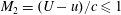
In contrast to the non-stationary flows, in the case of pseudo-steady flow, the corner is the only origin of disturbances communicating with the curved part of the reflected shock wave. This distinction has a major influence not only on the inter-shock-waves angle but also on the resulting thermodynamic properties near the reflection point. Figure 11 compares the reflection configurations obtained at a straight wedge with reflections obtained over the 40, 70 and 100 mm models at the same surface angle. In (a–d), the magnified schlieren images and the reflected shock wave orientation as was found automatically by the image-processing procedure are plotted. In pseudo-steady flows (figure 11
a), the two-shock theory predicts a
 $90^{\circ }$
angle between the incident and reflected shock waves when a wedge is inclined at an angle of
$90^{\circ }$
angle between the incident and reflected shock waves when a wedge is inclined at an angle of
 $47.5^{\circ }$
. This is consistent with the numerical results shown in figure 11(a). For the convex models, the radii dimensions clearly affect the reflected shock-wave orientations. As the radii dimension decreases, the orientation of the reflected shock wave deviates considerably from the horizontal line. The deviation is
$47.5^{\circ }$
. This is consistent with the numerical results shown in figure 11(a). For the convex models, the radii dimensions clearly affect the reflected shock-wave orientations. As the radii dimension decreases, the orientation of the reflected shock wave deviates considerably from the horizontal line. The deviation is
 $-3.9^{\circ }$
,
$-3.9^{\circ }$
,
 $-6.3^{\circ }$
and
$-6.3^{\circ }$
and
 $-7.5^{\circ }$
for the 100, 70 and 40 mm models, respectively. The radii dimensions clearly affect the reflected shock-wave orientations, which in turn controls the thermodynamic properties behind the reflected shock wave. This is demonstrated in figure 11(e–h), where the flow Mach number distributions with respect to the reflection point are presented. The minimum flow Mach numbers, obtained adjacent to the reflection point, increase when the radii dimension decreases. Thus, any correlation between the two-shock theory and non-stationary flows during the reflection process is questionable (Ben-Dor & Takayama Reference Ben-Dor and Takayama1986; Hakkaki-Fard & Timofeev Reference Hakkaki-Fard and Timofeev2012; Kleine et al.
Reference Kleine, Timofeev, Hakkaki-Fard and Skews2014).
$-7.5^{\circ }$
for the 100, 70 and 40 mm models, respectively. The radii dimensions clearly affect the reflected shock-wave orientations, which in turn controls the thermodynamic properties behind the reflected shock wave. This is demonstrated in figure 11(e–h), where the flow Mach number distributions with respect to the reflection point are presented. The minimum flow Mach numbers, obtained adjacent to the reflection point, increase when the radii dimension decreases. Thus, any correlation between the two-shock theory and non-stationary flows during the reflection process is questionable (Ben-Dor & Takayama Reference Ben-Dor and Takayama1986; Hakkaki-Fard & Timofeev Reference Hakkaki-Fard and Timofeev2012; Kleine et al.
Reference Kleine, Timofeev, Hakkaki-Fard and Skews2014).
Figure 11. Reflection over convex models having the same initial angle at a surface angle of
 $47.5^{\circ }$
and reflection over a wedge inclined at an angle of
$47.5^{\circ }$
and reflection over a wedge inclined at an angle of
 $47.5^{\circ }$
. The magnifications of the computational results and the reflected shock-wave orientation are shown in (a–d). The Mach number distributions calculated by the Mach-number-based technique are shown in (e–h). (a,e) straight wedge; (b,f)
$47.5^{\circ }$
. The magnifications of the computational results and the reflected shock-wave orientation are shown in (a–d). The Mach number distributions calculated by the Mach-number-based technique are shown in (e–h). (a,e) straight wedge; (b,f)
 $R=100~\text{mm}$
,
$R=100~\text{mm}$
,
 $\unicode[STIX]{x1D703}_{i}=60^{\circ }$
; (c,g)
$\unicode[STIX]{x1D703}_{i}=60^{\circ }$
; (c,g)
 $R=70~\text{mm}$
,
$R=70~\text{mm}$
,
 $\unicode[STIX]{x1D703}_{i}=60^{\circ }$
; (d,h)
$\unicode[STIX]{x1D703}_{i}=60^{\circ }$
; (d,h)
 $R=40~\text{mm}$
,
$R=40~\text{mm}$
,
 $\unicode[STIX]{x1D703}_{i}=60^{\circ }$
.
$\unicode[STIX]{x1D703}_{i}=60^{\circ }$
.
Since the RR evolution is dissimilar when considering pseudo-steady and non-stationary reflections, it is expected that the termination of an RR and the transition to an MR are not equivalent as well. Until now, locating the moment of transition was inherently difficult and imprecise. In many experimental studies, the RR
 $\rightarrow$
MR transition was determined to be the point where the Mach stem was first visualised. The Mach stem visualisation not only depends on the resolution of the experimental set-up but also locates the Mach stem long after its actual formation. High-resolution experiments may resolve the early stages of the Mach stem formation; however, the transition must be found by extrapolating the Mach stem length to zero. This extrapolation results in significant uncertainty originating from the low slope near the surface (Ram et al.
Reference Ram, Geva and Sadot2015). So far, a suitable criterion to locate the transition does not exist. Hakkaki-Fard & Timofeev (Reference Hakkaki-Fard and Timofeev2012) suggested that the criterion of the Mach-number-based technique is suitable for highly refined computations. According to this approach, when an RR exists, the entire flow along the surface in a frame of reference attached to the reflection point is supersonic. The MR evolves when a sonic point is reached, i.e. when at least one grid cell behind the reflected shock wave satisfies
$\rightarrow$
MR transition was determined to be the point where the Mach stem was first visualised. The Mach stem visualisation not only depends on the resolution of the experimental set-up but also locates the Mach stem long after its actual formation. High-resolution experiments may resolve the early stages of the Mach stem formation; however, the transition must be found by extrapolating the Mach stem length to zero. This extrapolation results in significant uncertainty originating from the low slope near the surface (Ram et al.
Reference Ram, Geva and Sadot2015). So far, a suitable criterion to locate the transition does not exist. Hakkaki-Fard & Timofeev (Reference Hakkaki-Fard and Timofeev2012) suggested that the criterion of the Mach-number-based technique is suitable for highly refined computations. According to this approach, when an RR exists, the entire flow along the surface in a frame of reference attached to the reflection point is supersonic. The MR evolves when a sonic point is reached, i.e. when at least one grid cell behind the reflected shock wave satisfies
 $M_{2}=(U-u)/c\leqslant 1$
, where
$M_{2}=(U-u)/c\leqslant 1$
, where
 $U$
is the reflection point velocity along the surface and
$U$
is the reflection point velocity along the surface and
 $u$
and
$u$
and
 $c$
are the flow velocity and speed of sound in the grid cell, respectively. Hakkaki-Fard & Timofeev (Reference Hakkaki-Fard and Timofeev2012) and Kleine et al. (Reference Kleine, Timofeev, Hakkaki-Fard and Skews2014) stated that when applying the above formulation on a highly refined grid, the transition angle approaches the pseudo-steady criterion. In the present work, we were able to replicate this phenomenon. However, a subsonic flow behind the reflected shock wave is a necessary condition for the existence of an MR but it is still an insufficient condition! Figure 12 demonstrates this claim.
$c$
are the flow velocity and speed of sound in the grid cell, respectively. Hakkaki-Fard & Timofeev (Reference Hakkaki-Fard and Timofeev2012) and Kleine et al. (Reference Kleine, Timofeev, Hakkaki-Fard and Skews2014) stated that when applying the above formulation on a highly refined grid, the transition angle approaches the pseudo-steady criterion. In the present work, we were able to replicate this phenomenon. However, a subsonic flow behind the reflected shock wave is a necessary condition for the existence of an MR but it is still an insufficient condition! Figure 12 demonstrates this claim.
For steady and pseudo-steady flows, the Mach-number-based technique is contradictory to the two-shock theory because it predicts an MR configuration in a domain in which only an RR exists. The transition angle corresponding to the detachment criterion at
 $M_{s}=1.3$
is
$M_{s}=1.3$
is
 $46.345^{\circ }$
. At a surface angle of
$46.345^{\circ }$
. At a surface angle of
 $46.35^{\circ }$
, an RR is still possible. According to the two-shock theory, the flow Mach number behind the reflected shock wave in the frame of reference attached to the reflection point is
$46.35^{\circ }$
, an RR is still possible. According to the two-shock theory, the flow Mach number behind the reflected shock wave in the frame of reference attached to the reflection point is
 $M_{2}=0.928$
. This is consistent with the numerical Mach number distribution computed by the above formulation (figure 12
a). In fact, the Mach-number-based technique predicts the transition at a higher surface angle in a domain in which only an RR is possible (figure 12
b). Because this criterion is not suitable for the steady and pseudo-steady flows, its use in non-stationary flows to determine the transition is arguable.
$M_{2}=0.928$
. This is consistent with the numerical Mach number distribution computed by the above formulation (figure 12
a). In fact, the Mach-number-based technique predicts the transition at a higher surface angle in a domain in which only an RR is possible (figure 12
b). Because this criterion is not suitable for the steady and pseudo-steady flows, its use in non-stationary flows to determine the transition is arguable.

Figure 12. Flow Mach number in the frame of reference attached to the reflection point: (a) numerical Mach number distribution at
 $\unicode[STIX]{x1D703}_{w}=46.35^{\circ }$
, and (b) analytical Mach number behind the reflected shock wave versus the surface angle for
$\unicode[STIX]{x1D703}_{w}=46.35^{\circ }$
, and (b) analytical Mach number behind the reflected shock wave versus the surface angle for
 $M_{s}=1.3$
.
$M_{s}=1.3$
.
The elementary difference between the pseudo-steady and non-stationary reflections is the fact the reflected shock wave continuously adjusts to the varying surface angle. Consequently, its orientation changes in time, which alters the RR solution from self-similarity. In order to examine this transient mechanism it is necessary to measure the reflected shock angle evolution during the shock propagation along the surface. Figure 13 depicts the reflected shock wave angles with respect to the incident shock-wave motion direction plotted against the flow time. The automatic image processing procedure (Geva et al. Reference Geva, Ram and Sadot2013) was modified to evaluate these angles by fitting a linear line to a small straight part of the reflected shock wave near the wall and measuring its orientation. It should be noted that this measurement is inherently difficult. Properly fitting a linear line obliges selecting the largest possible section of the reflected shock wave near the wall. However, accounting for a distance, which is too long, degrades the quality of the fitting since the reflected shock wave becomes curved. Based on these limitations, figure 13(a,b) for Mach number 1.3 was plotted using a 1 mm length of the reflected shock wave. Whereas figure 13(c), accounting for Mach number 1.5, was plotted using 0.3 mm since higher Mach number increases the curvature of the reflected shock wave. In order to fit a shorter section of the reflected shock wave, a higher-resolution simulation was conducted for Mach number 1.5. The errors in these measurements were assessed by fitting lines that were 20 % longer and 20 % shorter.

Figure 13. The variation in the reflected shock-wave angles, with respect to the horizontal line (
 $\unicode[STIX]{x1D6FC}$
), along the flow time (a)
$\unicode[STIX]{x1D6FC}$
), along the flow time (a)
 $R=70~\text{mm}$
,
$R=70~\text{mm}$
,
 $\unicode[STIX]{x1D703}_{i}=60^{\circ }$
,
$\unicode[STIX]{x1D703}_{i}=60^{\circ }$
,
 $M_{s}=1.3$
; (b)
$M_{s}=1.3$
; (b)
 $R=100~\text{mm}$
,
$R=100~\text{mm}$
,
 $\unicode[STIX]{x1D703}_{i}=60^{\circ }$
,
$\unicode[STIX]{x1D703}_{i}=60^{\circ }$
,
 $M_{s}=1.3$
; and (c)
$M_{s}=1.3$
; and (c)
 $R=70~\text{mm}$
,
$R=70~\text{mm}$
,
 $\unicode[STIX]{x1D703}_{i}=60^{\circ }$
,
$\unicode[STIX]{x1D703}_{i}=60^{\circ }$
,
 $M_{s}=1.5$
. The angle
$M_{s}=1.5$
. The angle
 $\unicode[STIX]{x1D6FC}$
is demonstrated in figure 10.
$\unicode[STIX]{x1D6FC}$
is demonstrated in figure 10.
As can be seen in figure 13, the reflected shock wave is compelled to change its orientation in time. During its propagation along the curved surface, the reflected shock wave does not only translates but also rotates about the reflection point. This phenomenon, which was overlooked in previous studies, is in complete contrast to pseudo-steady flows, in which the reflected shock wave has only a translation motion along the surface. This distinction is used for the modification of the 2ST which is presented in § 3.2.1. The modification is then successfully compared with the experimentally validated high-resolution numerical computations.
Another interesting observation, based on figure 13, is the inflection points that occur when the angle between the reflected shock wave and the incident shock-wave motion direction are zero. These inflections indicate that the reflected shock-wave rotation terminates when the waves are perpendicular. Just after the perpendicularity of the waves, the reflected shock wave continues to rotate. In § 3.2.2, a criterion for the non-stationary RR
 $\rightarrow$
MR transition will be given. As will be analytically explained by the ‘no penetration’ of the flow condition, the transition is at the moment in which the wave are perpendicular.
$\rightarrow$
MR transition will be given. As will be analytically explained by the ‘no penetration’ of the flow condition, the transition is at the moment in which the wave are perpendicular.
3.2.1 Modification of the standard 2ST for convex surfaces
In order to model correctly the reflections over curved surfaces, the curvature of the surface and the rotational velocity,
 $\dot{\unicode[STIX]{x1D6FC}}$
, must be attended. For the sake of the arguments that follow, the rotational velocity is evaluated as the time derivative of the angle
$\dot{\unicode[STIX]{x1D6FC}}$
, must be attended. For the sake of the arguments that follow, the rotational velocity is evaluated as the time derivative of the angle
 $\unicode[STIX]{x1D6FC}$
(i.e. slopes presented in figure 14). The rate at which the reflected shock wave changes its orientation depends on the radii dimensions. When radii are small, the reflected shock wave is forced to adjust itself faster to the changing conditions and therefore its rotation increases. Considering the above discussion, the fact that the reflected wave continually changes its orientation implies that additional physics, which is influenced by this non-inertial behaviour, must be considered.
$\unicode[STIX]{x1D6FC}$
(i.e. slopes presented in figure 14). The rate at which the reflected shock wave changes its orientation depends on the radii dimensions. When radii are small, the reflected shock wave is forced to adjust itself faster to the changing conditions and therefore its rotation increases. Considering the above discussion, the fact that the reflected wave continually changes its orientation implies that additional physics, which is influenced by this non-inertial behaviour, must be considered.

Figure 14. Inclination angle results for the cylindrical (a), (b), (d) models shown in figure 4 and elliptical model (a) shown in figure 5. The initial angle was not varied since it does not affect the transition (Kleine et al.
Reference Kleine, Timofeev, Hakkaki-Fard and Skews2014 and § 3.2.2). Inclination angle
 $\unicode[STIX]{x1D6FC}$
is defined in figure 10.
$\unicode[STIX]{x1D6FC}$
is defined in figure 10.
The standard 2ST, which is suitable for pseudo-steady reflections, is solved when the reference frame is attached to the reflection point. Thus, the shock waves are considered stationary and the flow passes through the waves (figure 1
b). Figure 15 illustrates the difference in the velocities entering the reflected shock waves when pseudo-steady and non-stationary RR are considered. In figure 15(a) the pseudo-steady RR configuration is presented. The flow enters the incident shock wave at
 $M_{0}$
and then it is deflected and is reduced to
$M_{0}$
and then it is deflected and is reduced to
 $M_{1}$
. So the flow that enters the reflected shock wave is
$M_{1}$
. So the flow that enters the reflected shock wave is
 $M_{1}$
(figure 15
b). When considering the RR over convex surface (figure 5
c), in addition to
$M_{1}$
(figure 15
b). When considering the RR over convex surface (figure 5
c), in addition to
 $M_{1}$
, the reflected shock wave advances towards the incident shock wave. As a result of this relative motion, an increase in the effective velocity that enters the reflected shock wave is obtained,
$M_{1}$
, the reflected shock wave advances towards the incident shock wave. As a result of this relative motion, an increase in the effective velocity that enters the reflected shock wave is obtained,
 $M_{1}^{\prime }$
(figure 15
d). Each point along the reflected shock wave has a different velocity entering the wave at a different angle.
$M_{1}^{\prime }$
(figure 15
d). Each point along the reflected shock wave has a different velocity entering the wave at a different angle.

Figure 15. Schematic description of the velocity field in domains 0 and 1 when the waves are considered stationary: (a) pseudo-steady RR and (b) velocity entering the reflected shock wave in pseudo-steady reflection. (c) Non-stationary RR and (d) velocity entering the reflected shock wave in non-stationary reflection.
 $a_{1}$
is the speed of sound at domain 1 and
$a_{1}$
is the speed of sound at domain 1 and
 $r$
is the distance from the reflection point.
$r$
is the distance from the reflection point.
 $\dot{\unicode[STIX]{x1D6FC}}$
is the rotational velocity obtained in figure 14.
$\dot{\unicode[STIX]{x1D6FC}}$
is the rotational velocity obtained in figure 14.
Another difference results from the curvature of the surface. Unlike the pseudo-steady case where the surface angle is constant (figure 16 a). In convex surfaces, the surface angle increases upstream from the reflection point. Since the incoming flow must be parallel to any local surface angle (‘no-penetration’ condition of the flow), the required deflection angle of the reflected shock wave is decreased along the wave (figure 16 b). Hence, the modified 2ST solution requires the modification of the velocity entering the reflected shock wave together with the modification of the required deflection angle. Since both depend of the distance from the reflection point, the reflected shock wave is divided into increments and the modification is calculated along each point.

Figure 16. Schematic description of the flow field behind the reflected shock wave (a) pseudo-steady reflection and (b) non-stationary reflections.
Modified 2ST. As regards the calculation of the flow conditions across the incident shock wave, the modified 2ST that will be discussed here does not require any different analysis from that used in the standard 2ST. The conditions behind the incident shock are obtained by solving the standard oblique shock-wave relations (setting
 $j=1$
and
$j=1$
and
 $i=0$
):
$i=0$
):
 $$\begin{eqnarray}\displaystyle & \displaystyle \unicode[STIX]{x1D703}_{j}=\tan ^{-1}\left[\frac{(M_{i}^{2}\sin ^{2}\unicode[STIX]{x1D719}_{j}-1)\cot \unicode[STIX]{x1D719}_{j}}{{\displaystyle \frac{\unicode[STIX]{x1D6FE}+1}{2}}M_{i}^{2}-(M_{i}^{2}\sin \unicode[STIX]{x1D719}_{j}-1)}\right], & \displaystyle\end{eqnarray}$$
 $$\begin{eqnarray}\displaystyle & \displaystyle M_{j}^{2}=\frac{\left[1+{\textstyle \frac{1}{2}}(\unicode[STIX]{x1D6FE}-1)M_{i}^{2}\sin ^{2}\unicode[STIX]{x1D719}_{j}\right]^{2}+\left[{\textstyle \frac{1}{4}}(\unicode[STIX]{x1D6FE}+1)M_{i}^{2}\sin 2\unicode[STIX]{x1D719}_{j}\right]^{2}}{\left[1+{\textstyle \frac{1}{2}}(\unicode[STIX]{x1D6FE}-1)M_{i}^{2}\sin ^{2}\unicode[STIX]{x1D719}_{j}\right]\left[\unicode[STIX]{x1D6FE}M_{i}^{2}\sin ^{2}\unicode[STIX]{x1D719}_{j}-{\textstyle \frac{1}{2}}(\unicode[STIX]{x1D6FE}-1)\right]}, & \displaystyle\end{eqnarray}$$
where
 $\unicode[STIX]{x1D719}_{1}=90^{\circ }-\unicode[STIX]{x1D703}_{w}$
,
$\unicode[STIX]{x1D719}_{1}=90^{\circ }-\unicode[STIX]{x1D703}_{w}$
,
 $M_{0}=M_{s}/\sin \unicode[STIX]{x1D719}_{1}$
and
$M_{0}=M_{s}/\sin \unicode[STIX]{x1D719}_{1}$
and
 $\unicode[STIX]{x1D6FE}$
is the heat capacities ratio. Figure 17 shows the velocity behind the shock,
$\unicode[STIX]{x1D6FE}$
is the heat capacities ratio. Figure 17 shows the velocity behind the shock,
 $M_{1}$
, and its orientation,
$M_{1}$
, and its orientation,
 $\unicode[STIX]{x1D719}_{1}-\unicode[STIX]{x1D703}_{1}$
. As for the reflected shock wave, consider an arbitrary point A along the reflected shock wave (figure 17). The effective velocity that enters the reflected shock wave is increased because of the relative motion of the waves. Consequently, the Mach number of the flow entering the reflected shock wave at an arbitrary point A is then calculated as follows:
$\unicode[STIX]{x1D719}_{1}-\unicode[STIX]{x1D703}_{1}$
. As for the reflected shock wave, consider an arbitrary point A along the reflected shock wave (figure 17). The effective velocity that enters the reflected shock wave is increased because of the relative motion of the waves. Consequently, the Mach number of the flow entering the reflected shock wave at an arbitrary point A is then calculated as follows:
 $$\begin{eqnarray}M_{1A}^{\prime }=\frac{|\bar{V}_{1}+\bar{\dot{\unicode[STIX]{x1D6FC}}}\times \bar{r}_{A}|}{a_{1}},\end{eqnarray}$$
where
 $a_{1}$
is the sound velocity behind the incident shock wave, and the fluid velocity
$a_{1}$
is the sound velocity behind the incident shock wave, and the fluid velocity
 $V_{1}=M_{1}/a_{1}$
is calculated in the reference frame attached to the reflection point. The orientation of
$V_{1}=M_{1}/a_{1}$
is calculated in the reference frame attached to the reflection point. The orientation of
 $r_{A}$
with respect to the incident shock-wave motion is initially estimated by a random value of
$r_{A}$
with respect to the incident shock-wave motion is initially estimated by a random value of
 $\unicode[STIX]{x1D6FC}$
. This value is then updated through an iterative procedure until a convergence of the energy equations was obtained. The required deflection angle through the reflected shock wave decreases and is modified as follows (figure 17):
$\unicode[STIX]{x1D6FC}$
. This value is then updated through an iterative procedure until a convergence of the energy equations was obtained. The required deflection angle through the reflected shock wave decreases and is modified as follows (figure 17):
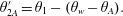 $$\begin{eqnarray}\unicode[STIX]{x1D703}_{2A}^{\prime }=\unicode[STIX]{x1D703}_{1}-(\unicode[STIX]{x1D703}_{w}-\unicode[STIX]{x1D703}_{A}).\end{eqnarray}$$
Note that the dependency of the reflecting surface on the curvature is embodied both in
 $\dot{\unicode[STIX]{x1D6FC}}$
and in the surface angle at point A. Previous analytical approaches, which were presented in the introduction, failed to integrate this dependence. Substituting the modifications of the flow Mach number and the required deflection angle, equation (3.1) with
$\dot{\unicode[STIX]{x1D6FC}}$
and in the surface angle at point A. Previous analytical approaches, which were presented in the introduction, failed to integrate this dependence. Substituting the modifications of the flow Mach number and the required deflection angle, equation (3.1) with
 $i=1$
and
$i=1$
and
 $j=2$
results in
$j=2$
results in
 $$\begin{eqnarray}\unicode[STIX]{x1D703}_{2A}^{\prime }=\tan ^{-1}\left[\frac{(M_{1A}^{\prime 2}\sin \unicode[STIX]{x1D719}_{2}-1)\cot \unicode[STIX]{x1D719}_{2}}{{\displaystyle \frac{\unicode[STIX]{x1D6FE}+1}{2}}M_{1A}^{\prime 2}-(M_{1A}^{\prime 2}\sin \unicode[STIX]{x1D719}_{2}-1)}\right].\end{eqnarray}$$
A better estimation for
 $\unicode[STIX]{x1D6FC}$
can be found as
$\unicode[STIX]{x1D6FC}$
can be found as
 $\unicode[STIX]{x1D6FC}=90^{\circ }-(\unicode[STIX]{x1D719}_{1}-\unicode[STIX]{x1D703}_{1})-\unicode[STIX]{x1D719}_{2}$
. The values of
$\unicode[STIX]{x1D6FC}=90^{\circ }-(\unicode[STIX]{x1D719}_{1}-\unicode[STIX]{x1D703}_{1})-\unicode[STIX]{x1D719}_{2}$
. The values of
 $M_{1A}^{\prime }$
and
$M_{1A}^{\prime }$
and
 $\unicode[STIX]{x1D703}_{2A}^{\prime }$
are updated with the improved estimation of
$\unicode[STIX]{x1D703}_{2A}^{\prime }$
are updated with the improved estimation of
 $\unicode[STIX]{x1D6FC}$
. Equation (3.5) can be solved again. One should note that if there is no change in the angle
$\unicode[STIX]{x1D6FC}$
. Equation (3.5) can be solved again. One should note that if there is no change in the angle
 $\unicode[STIX]{x1D6FC}$
, the solution converged and the conservation equations are satisfied. Following the modification, all the flow properties can now be evaluated with respect to point A. The entire flow field properties can be computed across the shock if the above-mentioned procedure is repeated over the entire reflected shock wave. For the reader’s convenience, a numerical example is presented in § A.1.
$\unicode[STIX]{x1D6FC}$
, the solution converged and the conservation equations are satisfied. Following the modification, all the flow properties can now be evaluated with respect to point A. The entire flow field properties can be computed across the shock if the above-mentioned procedure is repeated over the entire reflected shock wave. For the reader’s convenience, a numerical example is presented in § A.1.
Figure 17. Deflection mechanism and flow domains over a convex surface: velocities, wave angles and turn angles related to the oblique shock-wave relations.
Results of modification and discussion. Figure 18 depicts the analytical results (white lines) over the grey-scale results obtained by the numerical simulations. Figure 18(a–c) shows the full frame results for the cylindrical models. While figure 18(d–f) presents the magnification of the corresponding red squares in figure 18(a–c), respectively. Adjacent to the reflection point, a good agreement was obtained between the simulations and the analytical formulation. The reader should bear in mind that the rotational velocity used for the modification was estimated near the reflection point, where the reflected shock was reasonably straight. Maintaining this notion when the radii are small is more difficult because the wave rapidly grows and has a more pronounced curvature. However, the rotational velocity estimation seems to hold for a larger distance along the reflected shock wave as the radii of the model increases.

Figure 18. Modified 2ST calculated with
 $\dot{\unicode[STIX]{x1D6FC}}$
obtained in figure 14 (marked by a white line). (a–c) Show the original images from the simulations. (d–f) Denote the magnifications: (a,d)
$\dot{\unicode[STIX]{x1D6FC}}$
obtained in figure 14 (marked by a white line). (a–c) Show the original images from the simulations. (d–f) Denote the magnifications: (a,d)
 $R=40~\text{mm}$
,
$R=40~\text{mm}$
,
 $\unicode[STIX]{x1D703}_{i}=60^{\circ }$
, (b,e)
$\unicode[STIX]{x1D703}_{i}=60^{\circ }$
, (b,e)
 $R=70~\text{mm}$
,
$R=70~\text{mm}$
,
 $\unicode[STIX]{x1D703}_{i}=60^{\circ }$
; (c,f)
$\unicode[STIX]{x1D703}_{i}=60^{\circ }$
; (c,f)
 $R=100~\text{mm}$
,
$R=100~\text{mm}$
,
 $\unicode[STIX]{x1D703}_{i}=60^{\circ }$
.
$\unicode[STIX]{x1D703}_{i}=60^{\circ }$
.
Figure 19 shows a solution at which an optimal rotational velocity was found to yield the best correlation to the numerical results along a 2 mm distance. The rotational velocity that was found was lower than the previously computed
 $\dot{\unicode[STIX]{x1D6FC}}$
(figure 14). Figure 20 shows the optimal rotational velocities correlating to the numerical results at different distances along the reflected shock wave. The rotational velocity decreases when larger distances from the reflection point are considered. The same trend was obtained when the modified 2ST was applied for the elliptical model. The previously computed rotational velocity (figure 14) yielded a good correlation with the numerical results close to the reflection point (figure 21
a,d). One should use a smaller rotational velocity for the modified solution to be applicable further away. The reflected shock waves presented in figure 21(b,c,e,f) were calculated with optimal velocities. These rotational velocities were plotted against the distance from the reflection point (figure 22). Similar to the cylindrical models, the rotational velocity of the reflected shock decreased with the increased distance from the reflection point. Therefore, applying the rotational velocity that was found based on a small straight part close to the reflection point was not suitable (figure 14). From a physical perspective, the modification corresponding to the rotational speed is necessary. Yet, the mathematical question on the proper evaluation of the rotational speed along the reflected shock remains open. The rotational velocity evaluation is usually performed using continuum mechanics methods. However, applying it here is impossible because it requires the association of points on the reflected shock at different times. The authors believe that the ‘no-penetration’ condition of the flow, which is presented in the following section of this study, can serve as an additional equation to determine the rotational velocity at each point along the reflected shock wave. As long as the rotational velocity is known, the modified 2ST can be applied to any point along the reflected shock wave. Since the modification is based on the fundamental condition of ‘no penetration’ of the flow, it is not restricted to the area near the reflection point. Yet the crucial area that relates to the transition is the region adjacent to the reflection point.
$\dot{\unicode[STIX]{x1D6FC}}$
(figure 14). Figure 20 shows the optimal rotational velocities correlating to the numerical results at different distances along the reflected shock wave. The rotational velocity decreases when larger distances from the reflection point are considered. The same trend was obtained when the modified 2ST was applied for the elliptical model. The previously computed rotational velocity (figure 14) yielded a good correlation with the numerical results close to the reflection point (figure 21
a,d). One should use a smaller rotational velocity for the modified solution to be applicable further away. The reflected shock waves presented in figure 21(b,c,e,f) were calculated with optimal velocities. These rotational velocities were plotted against the distance from the reflection point (figure 22). Similar to the cylindrical models, the rotational velocity of the reflected shock decreased with the increased distance from the reflection point. Therefore, applying the rotational velocity that was found based on a small straight part close to the reflection point was not suitable (figure 14). From a physical perspective, the modification corresponding to the rotational speed is necessary. Yet, the mathematical question on the proper evaluation of the rotational speed along the reflected shock remains open. The rotational velocity evaluation is usually performed using continuum mechanics methods. However, applying it here is impossible because it requires the association of points on the reflected shock at different times. The authors believe that the ‘no-penetration’ condition of the flow, which is presented in the following section of this study, can serve as an additional equation to determine the rotational velocity at each point along the reflected shock wave. As long as the rotational velocity is known, the modified 2ST can be applied to any point along the reflected shock wave. Since the modification is based on the fundamental condition of ‘no penetration’ of the flow, it is not restricted to the area near the reflection point. Yet the crucial area that relates to the transition is the region adjacent to the reflection point.

Figure 19. Results of the modified 2ST (marked with white lines) calculated with the optimal rotational velocity,
 $\dot{\unicode[STIX]{x1D6FC}}^{opt}$
. (a–c) Show the original images from the simulations. (d–f) Denote the magnifications. (a,d)
$\dot{\unicode[STIX]{x1D6FC}}^{opt}$
. (a–c) Show the original images from the simulations. (d–f) Denote the magnifications. (a,d)
 $R=40~\text{mm}$
,
$R=40~\text{mm}$
,
 $\unicode[STIX]{x1D703}_{i}=60^{\circ }$
; (b,e)
$\unicode[STIX]{x1D703}_{i}=60^{\circ }$
; (b,e)
 $R=70~\text{mm}$
,
$R=70~\text{mm}$
,
 $\unicode[STIX]{x1D703}_{i}=60^{\circ }$
; and (c,f)
$\unicode[STIX]{x1D703}_{i}=60^{\circ }$
; and (c,f)
 $R=100~\text{mm}$
,
$R=100~\text{mm}$
,
 $\unicode[STIX]{x1D703}_{i}=60^{\circ }$
.
$\unicode[STIX]{x1D703}_{i}=60^{\circ }$
.

Figure 20. Optimum rotational velocity as a function of the distance from the reflection point,
 $d$
, over cylindrical models.
$d$
, over cylindrical models.

Figure 21. Results of the modified 2ST (marked by white lines) applied to the reflection over the ellipse. (a–c) Denote the original images from the simulations. (d–f) Present the magnifications. (a,d) Modified 2ST with computed in figure 14; (b,e) modified 2ST with the optimal rotational velocity for 2 mm length; and (c,f) modified 2ST with the optimal rotational velocity for the 4 mm length.

Figure 22. Optimum rotational velocity as a function of the distance from the reflection point,
 $d$
, over the ellipse.
$d$
, over the ellipse.
Figure 23(a) presents a comparison between the standard 2ST and the modified 2ST over a 70 mm cylinder. The radial velocity and the deflection angle corrections depend on the distance from the reflection point. Therefore, a very small correction is required. This deviation increases from the reflection point. Figure 23(b) graphically demonstrates the deviation by the shock polars. The
 $r$
-polar of the modified 2ST starts at
$r$
-polar of the modified 2ST starts at
 $\unicode[STIX]{x1D703}_{2}^{\prime }$
, which is smaller than
$\unicode[STIX]{x1D703}_{2}^{\prime }$
, which is smaller than
 $\unicode[STIX]{x1D703}_{2}$
. In addition, the flow Mach number of the modified polar,
$\unicode[STIX]{x1D703}_{2}$
. In addition, the flow Mach number of the modified polar,
 $M_{1}^{\prime }$
, is larger than that of the flow Mach number computed by the standard 2ST,
$M_{1}^{\prime }$
, is larger than that of the flow Mach number computed by the standard 2ST,
 $M_{1}$
. The two-shock solution is obtained at the intersection of the
$M_{1}$
. The two-shock solution is obtained at the intersection of the
 $r$
-polar with the vertical axis. One can see that the
$r$
-polar with the vertical axis. One can see that the
 $p_{2}^{\prime }/p_{1}<p_{2}/p_{1}$
.
$p_{2}^{\prime }/p_{1}<p_{2}/p_{1}$
.

Figure 23. The difference between the standard and modified 2ST. (a) Resulting reflected shock wave obtained by the standard 2ST and by the modified 2ST over a 70 mm model. (b) Polar representation of the solutions.
These modified conditions make it easier for the flow to be deflected. Consequently, the RR can be retained for smaller surface angles in comparison with pseudo-steady flows. This explanation sheds new light on the transition criterion disagreements between the pseudo-steady and unsteady reflections. As the effective flow entering the reflected shock wave is increased and the required deflection angle is decreased, the reflected shock-wave angle and the induced flow behind the reflected shock are decreased (for further explanation see § A.2). The rotation of the reflected shock wave alters the effective flow Mach number entering the reflected wave. This velocity is determined so the ‘no-penetration’ condition is maintained (as will be shown in the next section). For smaller radii, the rapid change in the surface angles affects both
 $\dot{\unicode[STIX]{x1D6FC}}$
and the required deflection angle,
$\dot{\unicode[STIX]{x1D6FC}}$
and the required deflection angle,
 $\unicode[STIX]{x1D703}_{2}^{\prime }$
. Hence, a significant modification is needed and the delay in the transition will be more noticeable. This finding is consistent with the observation that the radius of curvature is the only available length scale over curved surfaces (Ram et al.
Reference Ram, Geva and Sadot2015) and strengthens the claim that the transition angles depend of the radius of curvature (Takayama & Sasaki Reference Takayama and Sasaki1983; Ben-Dor Reference Ben-Dor2007). No difference between the pseudo-steady and unsteady reflections was observed near the reflection point. Nevertheless, these data are insufficient in determining whether the transition criteria are similar (Hakkaki-Fard & Timofeev Reference Hakkaki-Fard and Timofeev2012; Kleine et al.
Reference Kleine, Timofeev, Hakkaki-Fard and Skews2014). Basing the transition criterion on the conditions very close to the reflection point is insufficient because the zone behind the reflection point that leads to the transition is unknown. Moreover, their observation that coarser grid numerical results depart from the pseudo-steady results can also be explained now. The shock waves in coarser grids tend to be thicker. Therefore, they force a large artificial modification in the required deflection angles,
$\unicode[STIX]{x1D703}_{2}^{\prime }$
. Hence, a significant modification is needed and the delay in the transition will be more noticeable. This finding is consistent with the observation that the radius of curvature is the only available length scale over curved surfaces (Ram et al.
Reference Ram, Geva and Sadot2015) and strengthens the claim that the transition angles depend of the radius of curvature (Takayama & Sasaki Reference Takayama and Sasaki1983; Ben-Dor Reference Ben-Dor2007). No difference between the pseudo-steady and unsteady reflections was observed near the reflection point. Nevertheless, these data are insufficient in determining whether the transition criteria are similar (Hakkaki-Fard & Timofeev Reference Hakkaki-Fard and Timofeev2012; Kleine et al.
Reference Kleine, Timofeev, Hakkaki-Fard and Skews2014). Basing the transition criterion on the conditions very close to the reflection point is insufficient because the zone behind the reflection point that leads to the transition is unknown. Moreover, their observation that coarser grid numerical results depart from the pseudo-steady results can also be explained now. The shock waves in coarser grids tend to be thicker. Therefore, they force a large artificial modification in the required deflection angles,
 $\unicode[STIX]{x1D703}_{2}^{\prime }$
. The MR is eventually formed when the RR can no longer sustain the required deflection of the flow. Consequently, in unsteady reflections, the increase in the flow Mach number along with the decrease in the required deflection angle will delay the transition.
$\unicode[STIX]{x1D703}_{2}^{\prime }$
. The MR is eventually formed when the RR can no longer sustain the required deflection of the flow. Consequently, in unsteady reflections, the increase in the flow Mach number along with the decrease in the required deflection angle will delay the transition.
3.2.2 The physical mechanism that leads to transition at
 $90^{\circ }$
inter-shock-waves angle
$90^{\circ }$
inter-shock-waves angle

The RR configuration is formed so that a supersonic flow can be negotiated about an obstacle. Consider the pseudo steady flow that is shown in figure 24. The induced flow behind the reflected shock wave,
 $u_{2}$
, is parallel to the surface and the velocity component, which is perpendicular to the surface, is therefore zero (‘no-penetration’ condition).
$u_{2}$
, is parallel to the surface and the velocity component, which is perpendicular to the surface, is therefore zero (‘no-penetration’ condition).

Figure 24. Schematic description of the flow regions in pseudo-steady RR.
The flow velocity along the surface behind the reflected shock wave in region 2 is given by:
 $$\begin{eqnarray}u_{2}=\unicode[STIX]{x0394}u_{i}\sin \unicode[STIX]{x1D719}_{1}+\unicode[STIX]{x0394}u_{r}\sin \unicode[STIX]{x1D703}_{r},\end{eqnarray}$$
where
 $\unicode[STIX]{x0394}u_{i}$
and
$\unicode[STIX]{x0394}u_{i}$
and
 $\unicode[STIX]{x0394}u_{r}$
are the induced flow velocities from the incident and the reflected shock waves, respectively. Due to the ‘no-penetration’ condition, the normal components of the induced flow velocities of the incident and reflected shock waves counter each other:
$\unicode[STIX]{x0394}u_{r}$
are the induced flow velocities from the incident and the reflected shock waves, respectively. Due to the ‘no-penetration’ condition, the normal components of the induced flow velocities of the incident and reflected shock waves counter each other:
 $$\begin{eqnarray}\unicode[STIX]{x0394}u_{i}\cos \unicode[STIX]{x1D719}_{1}=\unicode[STIX]{x0394}u_{r}\cos \unicode[STIX]{x1D703}_{r}.\end{eqnarray}$$
Hryniewicki, Gottlieb & Groth (Reference Hryniewicki, Gottlieb and Groth2016) used (3.7) and constructed an error function
 $$\begin{eqnarray}E(\unicode[STIX]{x1D703}_{r})=1-\frac{\unicode[STIX]{x0394}u_{r}\cos \unicode[STIX]{x1D703}_{r}}{\unicode[STIX]{x0394}u_{i}\cos \unicode[STIX]{x1D719}_{1}}.\end{eqnarray}$$
When this equals zero a solution for a regular reflection occurs. In other words, the reflected shock-wave angle is chosen in order to maintain the geometrical ‘no-penetration’ requirement.

Figure 25. Unsteady RR configuration in which the reflected and incident shock waves are perpendicular.
The elementary requirement that the flow will not penetrate the surface exists in both pseudo-steady and unsteady flows. The particular moment at which the reflected shock becomes perpendicular to the incident shock wave was found to be the moment at which the RR
 $\rightarrow$
MR transition occurs. An explanation to this finding is that at this perpendicular angle equation (3.8) becomes identically zero. (This moment is illustrated in figure 25.):
$\rightarrow$
MR transition occurs. An explanation to this finding is that at this perpendicular angle equation (3.8) becomes identically zero. (This moment is illustrated in figure 25.):
 $$\begin{eqnarray}1-\frac{\unicode[STIX]{x0394}u_{r}}{\unicode[STIX]{x0394}u_{i}}\frac{\cos \unicode[STIX]{x1D703}_{r}}{\cos \unicode[STIX]{x1D719}_{1}}=1-\tan \unicode[STIX]{x1D703}_{w}\frac{\cos \unicode[STIX]{x1D703}_{w}}{\cos (90-\unicode[STIX]{x1D703}_{w})}=1-\tan \unicode[STIX]{x1D703}_{w}\frac{\cos \unicode[STIX]{x1D703}_{w}}{\sin \unicode[STIX]{x1D703}_{w}}=0.\end{eqnarray}$$
Before the transition, in order for the ‘no-penetration’ condition to be held, a rotational velocity of the reflected shock wave must be introduced. This velocity causes an increase in the effective flow Mach number entering the reflected shock wave. As a result, the reflected shock-wave angle and the induced flow behind the reflected wave are reduced so (3.8) is maintained. The analytical justification is consistent with the findings presented in figure 11. As the radius decreases, higher rotational velocities are involved enabling the configuration to adjust quickly to the changing surface. This in turn is possible only if the angle between the reflected and incident shock waves increases.
The particular
 $90^{\circ }$
inter angle between the incident and reflected shock waves enables the existence of an RR without the need of an additional rotational velocity. Indeed, it was demonstrated in figure 13 that when the reflected shock wave is perpendicular to the incident shock wave, the rotation of the reflected shock wave reaches zero. Soon after, the reflected shock wave is no longer perpendicular to the incident shock wave. The only way to enable an RR, so that (3.8) is held, is by introducing an additional rotational velocity of the reflected shock wave. Due to the inertial movement of the flow around the shock wave, the buildup of the rotational velocity cannot transpire immediately. The delay in the rotational velocity buildup is demonstrated in the inflections of the rotational velocity shown in figure 13. Since an RR cannot deflect the flow so that ‘no-penetration’ condition is held, MR is then formed. The geometrical fundamental obligation of ‘no penetration’ is the criterion for the RR
$90^{\circ }$
inter angle between the incident and reflected shock waves enables the existence of an RR without the need of an additional rotational velocity. Indeed, it was demonstrated in figure 13 that when the reflected shock wave is perpendicular to the incident shock wave, the rotation of the reflected shock wave reaches zero. Soon after, the reflected shock wave is no longer perpendicular to the incident shock wave. The only way to enable an RR, so that (3.8) is held, is by introducing an additional rotational velocity of the reflected shock wave. Due to the inertial movement of the flow around the shock wave, the buildup of the rotational velocity cannot transpire immediately. The delay in the rotational velocity buildup is demonstrated in the inflections of the rotational velocity shown in figure 13. Since an RR cannot deflect the flow so that ‘no-penetration’ condition is held, MR is then formed. The geometrical fundamental obligation of ‘no penetration’ is the criterion for the RR
 $\rightarrow$
MR transition in unsteady reflection.
$\rightarrow$
MR transition in unsteady reflection.
The use of a highly refined computational mesh and high-resolution experiments enabled us to observe that this intriguing behaviour happened near the RR
 $\rightarrow$
MR transition. It was evident from both methods that an MR could not be formed if the angle between the incident and reflected shock waves was larger than
$\rightarrow$
MR transition. It was evident from both methods that an MR could not be formed if the angle between the incident and reflected shock waves was larger than
 $90^{\circ }$
. It was very difficult to decide if this
$90^{\circ }$
. It was very difficult to decide if this
 $90^{\circ }$
angle was the precise angle at transition considering the above listed methods to determined transition. However, based on the high-resolution findings, it was reasonable to assume that the transition occurred very close to this point at moderate incident shock-wave Mach numbers.
$90^{\circ }$
angle was the precise angle at transition considering the above listed methods to determined transition. However, based on the high-resolution findings, it was reasonable to assume that the transition occurred very close to this point at moderate incident shock-wave Mach numbers.
Figure 26 depicts the perpendicular behaviour of the reflected and incident shock waves for reflections over models (a–d) near the transition point. Corresponding to the inflections in figure 13, the perpendicularity was observed to sustain over a certain period. The ranges of the corresponding surface angles at which this behaviour was evident are given in table 1. Optical limitations and changing the simulation time increments may slightly vary these ranges. Geometrical dependence of the perpendicularity is obtained in term of a slight increase in the transition angle when the radius of the model increases. For cylindrical model (d), which has a 100 mm radius, the transition was found to be similar to the pseudo-steady criterion. The effect of the initial angle on the transition angle was also examined by using two models having 70 mm radii and initial angles of
 $60$
and
$60$
and
 $90^{\circ }$
. Similar to the findings in Skews & Kleine (Reference Skews and Kleine2010), it was found that the initial angle did not influence the transition. Figures 26(f) and 26(h) show the magnification of the red regions shown in figures 26(b) and 26(d), respectively. The horizontal behaviour of the reflected shock waves adjacent to the reflection is apparent at the same surface angle (table 1). This also reinforces the notion that the perpendicularity of the waves and the corresponding transition depends on the geometric scaling.
$90^{\circ }$
. Similar to the findings in Skews & Kleine (Reference Skews and Kleine2010), it was found that the initial angle did not influence the transition. Figures 26(f) and 26(h) show the magnification of the red regions shown in figures 26(b) and 26(d), respectively. The horizontal behaviour of the reflected shock waves adjacent to the reflection is apparent at the same surface angle (table 1). This also reinforces the notion that the perpendicularity of the waves and the corresponding transition depends on the geometric scaling.

Figure 26. Simulation results for reflections over models (a–d) near the transition angles (table 1). The original images from the computations are shown in (a–d). The magnification of the areas marked by red squares of the results and the reflected shock-wave orientation as extracted by the program are shown in (e–h). (a,e)
 $R=40~\text{mm}$
,
$R=40~\text{mm}$
,
 $\unicode[STIX]{x1D703}_{i}=60^{\circ }$
,
$\unicode[STIX]{x1D703}_{i}=60^{\circ }$
,
 $\unicode[STIX]{x1D703}_{w}=45.4^{\circ }$
; (b,f)
$\unicode[STIX]{x1D703}_{w}=45.4^{\circ }$
; (b,f)
 $R=70~\text{mm}$
,
$R=70~\text{mm}$
,
 $\unicode[STIX]{x1D703}_{i}=60^{\circ }$
,
$\unicode[STIX]{x1D703}_{i}=60^{\circ }$
,
 $\unicode[STIX]{x1D703}_{w}=45.8^{\circ }$
; (c,g)
$\unicode[STIX]{x1D703}_{w}=45.8^{\circ }$
; (c,g)
 $R=100~\text{mm}$
,
$R=100~\text{mm}$
,
 $\unicode[STIX]{x1D703}_{i}=60^{\circ }$
,
$\unicode[STIX]{x1D703}_{i}=60^{\circ }$
,
 $\unicode[STIX]{x1D703}_{w}=46.3^{\circ }$
; (d,h)
$\unicode[STIX]{x1D703}_{w}=46.3^{\circ }$
; (d,h)
 $R=70~\text{mm}$
,
$R=70~\text{mm}$
,
 $\unicode[STIX]{x1D703}_{i}=90^{\circ }$
,
$\unicode[STIX]{x1D703}_{i}=90^{\circ }$
,
 $\unicode[STIX]{x1D703}_{w}=45.8^{\circ }$
.
$\unicode[STIX]{x1D703}_{w}=45.8^{\circ }$
.
Table 1. Surface angles corresponding to the horizontal behaviour of the reflected shock wave over cylindrical surfaces.

a The upper boundary of the theoretical error is limited by the detachment criterion.
For the case of reflections over the elliptical models, a geometric scaling was also observed. In these cases, due to the varying curvature, a varying rate of change is imposed on the transition process. Table 2 presents the surface angles of the ellipses corresponding to the moment in which the perpendicularity behaviour of the shock waves was observed. Figure 27 demonstrates the perpendicularity of the reflected and incident shock waves over the elliptical models. For the ellipse with a decreasing radius of curvature (model b), the transition angle is closer to the detachment criterion and is similar to the transition angle found for reflections over the 100 mm cylindrical model. For the elliptical model with an increasing radius of curvature (model a), the transition angle is similar to the transition angle obtained for reflections over the 70 mm cylindrical model. This deviation implies that geometrical scaling may be a solution to eliminate this discrepancy. Using Pratt (Reference Pratt1987) method, a circle was fitted to the area after the transition to describe the MR growth (figure 28), and the scale that was found appropriate for the transition was the best-fit circle prior to the transition (
 $46^{\circ }\leqslant \unicode[STIX]{x1D703}_{w}\leqslant 60^{\circ }$
). The radii of the resulting equivalent circles are 68 and 93 mm for models (a) and (b), respectively (figure 28). In fact, as long as a circle can be fitted, the surface curvature does not play a role in the determination of the transition.
$46^{\circ }\leqslant \unicode[STIX]{x1D703}_{w}\leqslant 60^{\circ }$
). The radii of the resulting equivalent circles are 68 and 93 mm for models (a) and (b), respectively (figure 28). In fact, as long as a circle can be fitted, the surface curvature does not play a role in the determination of the transition.

Figure 27. Simulation results for reflections over elliptical models near the transition (table 2). (a,b) The original images obtained by the computations. (c,d) The magnification of the areas marked by red squares and the reflected shock-wave orientation extracted by the program. (a,c)
 $a=150~\text{mm}$
,
$a=150~\text{mm}$
,
 $b=70~\text{mm}$
,
$b=70~\text{mm}$
,
 $\unicode[STIX]{x1D703}_{i}=60^{\circ }$
,
$\unicode[STIX]{x1D703}_{i}=60^{\circ }$
,
 $\unicode[STIX]{x1D703}_{w}=45.8^{\circ }$
; (b,d)
$\unicode[STIX]{x1D703}_{w}=45.8^{\circ }$
; (b,d)
 $a=70~\text{mm}$
,
$a=70~\text{mm}$
,
 $b=150~\text{mm}$
,
$b=150~\text{mm}$
,
 $\unicode[STIX]{x1D703}_{i}=90^{\circ }$
,
$\unicode[STIX]{x1D703}_{i}=90^{\circ }$
,
 $\unicode[STIX]{x1D703}_{w}=46.2^{\circ }$
.
$\unicode[STIX]{x1D703}_{w}=46.2^{\circ }$
.

Figure 28. Best-fit circle to the ellipse in the area prior to the transition at surfaces angles
 $46^{\circ }\leqslant \unicode[STIX]{x1D703}_{w}\leqslant 60^{\circ }$
: (a) a circle with a 68 mm radius is fitted to an ellipse with an increasing radius of curvature, and (b) a circle with a 93 mm radius is fitted to an ellipse with a decreasing radius of curvature.
$46^{\circ }\leqslant \unicode[STIX]{x1D703}_{w}\leqslant 60^{\circ }$
: (a) a circle with a 68 mm radius is fitted to an ellipse with an increasing radius of curvature, and (b) a circle with a 93 mm radius is fitted to an ellipse with a decreasing radius of curvature.
Table 2. Surface angles corresponding to the horizontal behaviour of the reflected shock wave over elliptical surfaces.

Figure 29 demonstrates the perpendicularity of the reflected shock wave near the transition points that was obtained experimentally. The Mach stems were measured in the following frames, and the angles between the incident and reflected shock waves were found to be smaller than
 $90^{\circ }$
. Figure 29(g) demonstrates the inflection process as was obtained experimentally. The surface angles at which the reflected shock wave was horizontal, i.e. perpendicular to the incident shock wave, were found to be consistent with the transition angles obtained by extrapolation, with the former method having the advantage of producing smaller uncertainties.
$90^{\circ }$
. Figure 29(g) demonstrates the inflection process as was obtained experimentally. The surface angles at which the reflected shock wave was horizontal, i.e. perpendicular to the incident shock wave, were found to be consistent with the transition angles obtained by extrapolation, with the former method having the advantage of producing smaller uncertainties.

Figure 29. Experimental results for reflections over cylindrical models at angles at which the reflected shock is horizontal. (a–c) The original images from the experiments. (d–f) The magnification of the areas marked by red squares of the results and the reflected shock-wave orientation. (a,d)
 $R=70~\text{mm}$
,
$R=70~\text{mm}$
,
 $\unicode[STIX]{x1D703}_{i}=60^{\circ }$
,
$\unicode[STIX]{x1D703}_{i}=60^{\circ }$
,
 $\unicode[STIX]{x1D703}_{w}\approx 45^{\circ }$
; (b,e)
$\unicode[STIX]{x1D703}_{w}\approx 45^{\circ }$
; (b,e)
 $R=70~\text{mm}$
,
$R=70~\text{mm}$
,
 $\unicode[STIX]{x1D703}_{i}=90^{\circ }$
,
$\unicode[STIX]{x1D703}_{i}=90^{\circ }$
,
 $\unicode[STIX]{x1D703}_{w}\approx 45^{\circ }$
; (c,f)
$\unicode[STIX]{x1D703}_{w}\approx 45^{\circ }$
; (c,f)
 $R=100~\text{mm}$
,
$R=100~\text{mm}$
,
 $\unicode[STIX]{x1D703}_{i}=60^{\circ }$
,
$\unicode[STIX]{x1D703}_{i}=60^{\circ }$
,
 $\unicode[STIX]{x1D703}_{w}\approx 46^{\circ }$
; (g) variation of the reflected shock-wave angle along the surface for
$\unicode[STIX]{x1D703}_{w}\approx 46^{\circ }$
; (g) variation of the reflected shock-wave angle along the surface for
 $R=70~\text{mm}$
,
$R=70~\text{mm}$
,
 $\unicode[STIX]{x1D703}_{i}=60^{\circ }$
.
$\unicode[STIX]{x1D703}_{i}=60^{\circ }$
.
The perpendicularity that was found to exist in both experiments and simulations could be regarded as a geometrical criterion for the RR
 $\rightarrow$
MR transition. Incidentally, this
$\rightarrow$
MR transition. Incidentally, this
 $90^{\circ }$
condition is similar to the condition suggested by Shirouzu & Glass (Reference Shirouzu and Glass1986) for the transition between a single Mach reflection and transitional Mach reflection in pseudo-steady reflections. Until now, the rotation of the reflected shock wave was not considered significant and its existence was neglected. However, it was demonstrated that the rotation of the reflected shock wave affects the RR evolution and its termination. The RR evolution and transition to MR waves are perpendicular, stem from the ‘no penetration’ of the flow condition. Which is a fundamental condition that must be held for any flow that passes over any solid body. While performing experiments, it is considerably easier to visualise the perpendicularity of the reflected and incident shock waves. Rather than the incorrect determination based on the appearance of a Mach stem or to carry out the more complicated and uncertain task of measuring the Mach stem length and extrapolating it to zero (Kleine et al.
Reference Kleine, Timofeev, Hakkaki-Fard and Skews2014; Ram et al.
Reference Ram, Geva and Sadot2015).
$90^{\circ }$
condition is similar to the condition suggested by Shirouzu & Glass (Reference Shirouzu and Glass1986) for the transition between a single Mach reflection and transitional Mach reflection in pseudo-steady reflections. Until now, the rotation of the reflected shock wave was not considered significant and its existence was neglected. However, it was demonstrated that the rotation of the reflected shock wave affects the RR evolution and its termination. The RR evolution and transition to MR waves are perpendicular, stem from the ‘no penetration’ of the flow condition. Which is a fundamental condition that must be held for any flow that passes over any solid body. While performing experiments, it is considerably easier to visualise the perpendicularity of the reflected and incident shock waves. Rather than the incorrect determination based on the appearance of a Mach stem or to carry out the more complicated and uncertain task of measuring the Mach stem length and extrapolating it to zero (Kleine et al.
Reference Kleine, Timofeev, Hakkaki-Fard and Skews2014; Ram et al.
Reference Ram, Geva and Sadot2015).
3.3 Geometry governing Mach stem growth over convex surfaces
Following the formation of the MR, the obtained wave configuration is a direct Mach reflection and the Mach stem grows as the surface angle decreases (Ben-Dor Reference Ben-Dor2007). The triple point trajectories obtained from the simulations are plotted in figure 30(a). For cylindrical models, having a large radius of curvature, the growth of the Mach stems is faster than that for smaller radii. This is expected because as the radius increases, the amount of flow that must be deflected also increases. The similarity between our case and that of Kleine et al. (Reference Kleine, Timofeev, Hakkaki-Fard and Skews2014) enabled us to normalise the Mach stem length with the cylinder radius. The resulting normalised triple point trajectories are plotted in figure 30(b). The most noteworthy observation is that a change in the initial angle, i.e.
 $60^{\circ }$
and
$60^{\circ }$
and
 $90^{\circ }$
, does not affect the Mach stem growth, as can be seen in figure 30(a), where both the curves for the 70 mm radius coincide (triangular markers). The joined normalised curve demonstrates the consistent behaviour of the Mach stem growth over cylindrical convex surfaces having different radii of curvature and initial angles.
$90^{\circ }$
, does not affect the Mach stem growth, as can be seen in figure 30(a), where both the curves for the 70 mm radius coincide (triangular markers). The joined normalised curve demonstrates the consistent behaviour of the Mach stem growth over cylindrical convex surfaces having different radii of curvature and initial angles.

Figure 30. Simulation results of the Mach stem length for reflections over cylindrical and elliptical models: (a) Mach stem length versus the corresponding surface angle and (b) normalised Mach stem length versus the corresponding surface angle.
Regarding the elliptical models, both the trajectories for reflections over the elliptical surfaces fall within the trajectories of the cylindrical models. It is interesting to note that the normalisation parameter was not related to the geometrical shape of the ellipse. Different parameters that were ellipse oriented were examined, e.g. radius of curvature, distance from foci and in-circles. However, none of them was suitable. Surprisingly, the appropriate normalisation scale was the radius of the best-fit circle at surface angles in the range
 $30^{\circ }\leqslant \unicode[STIX]{x1D703}_{w}\leqslant 45^{\circ }$
. The circles were obtained using the Pratt method (Pratt Reference Pratt1987), and the computed circles are plotted in figure 31. The suitable normalisation radii were 95 and 54 mm for ellipses (a) and (b), respectively (figure 31). The normalised trajectories of the elliptical models coincide with those of the cylindrical models. This significant finding leads to the conclusion that regardless of the geometrical shape and its characteristic size, if a circle can be fitted, the growth of the Mach stem can be found.
$30^{\circ }\leqslant \unicode[STIX]{x1D703}_{w}\leqslant 45^{\circ }$
. The circles were obtained using the Pratt method (Pratt Reference Pratt1987), and the computed circles are plotted in figure 31. The suitable normalisation radii were 95 and 54 mm for ellipses (a) and (b), respectively (figure 31). The normalised trajectories of the elliptical models coincide with those of the cylindrical models. This significant finding leads to the conclusion that regardless of the geometrical shape and its characteristic size, if a circle can be fitted, the growth of the Mach stem can be found.

Figure 31. Best-fit circle to the ellipse in the area just after transition at surface angles in the range
 $45^{\circ }\leqslant \unicode[STIX]{x1D703}_{w}\leqslant 30^{\circ }$
: (a) a circle with a 95 mm radius fitted to an ellipse with an increasing radius of curvature, and (b) a circle with a 54 mm radius fitted to an ellipse with a decreasing radius of curvature.
$45^{\circ }\leqslant \unicode[STIX]{x1D703}_{w}\leqslant 30^{\circ }$
: (a) a circle with a 95 mm radius fitted to an ellipse with an increasing radius of curvature, and (b) a circle with a 54 mm radius fitted to an ellipse with a decreasing radius of curvature.


The aforementioned finding also reinforces the difference between pseudo-steady and non-stationary reflections in which a circle can never be fitted to a straight wedge. Conversely, the simplification of a circle-like assumption is not suitable for larger Mach stems. As the Mach stem grows, it is influenced not only by the surface curve but also by far-field effects. Therefore, additional parameters must be accounted for when evaluating the Mach stem length at smaller surface angles when the Mach stem is no longer perpendicular.
To find the geometrical parameters that influence the Mach stem buildup, several parameters were analysed. It was found that neither the initial angle nor the varying rate of curvature change is related to the buildup. Instead, the only geometrical dependency is in the radius of the surface. Even when considering a non-circular shape, the problem can be normalised by finding the best-fit circle. This geometrical dependence in the Mach stem growth is consistent with the geometrical dependence found to be dominant when RR was evident. This simple geometrical dependence reduces the complexity of the analysis of the reflection over convex surfaces and the complexity in the RR
 $\rightarrow$
MR transition in particular.
$\rightarrow$
MR transition in particular.
4 Conclusions
In this study, the non-stationary reflections over cylindrical and elliptical convex models were analysed numerically. Numerical computations were validated by experiments with extremely high spatial resolutions, thus enabling features as small as 0.06 mm to be resolved. The influence of the radius of the surface, initial angle, and varying rates of surface change were examined in the context of the RR evolution, RR
 $\rightarrow$
MR transition and Mach stem growth. It was found that the only geometrical parameter that affected the reflected is the radios of the surface. Regardless of the geometry involved, as long as a circle could be fitted to the surface, the radius of the best-fit circle was the characteristic length of the problem. This simplification eliminated all kinds of geometrical shape–oriented parameters and reduced the problem complexity considerably.
$\rightarrow$
MR transition and Mach stem growth. It was found that the only geometrical parameter that affected the reflected is the radios of the surface. Regardless of the geometry involved, as long as a circle could be fitted to the surface, the radius of the best-fit circle was the characteristic length of the problem. This simplification eliminated all kinds of geometrical shape–oriented parameters and reduced the problem complexity considerably.
Unlike the self-similarity in pseudo-steady reflections, in non-stationary flows the reflection configuration is not self-similar. The curved surface imposes the reflected shock wave a changing boundary conditions. The reflected shock orientation is varied as it responds to the continuous change in the surface angle. For the first time, the existence of the reflected shock-wave rotation about the reflection point was examined. This behaviour was demonstrated at Mach numbers 1.3 and 1.5. Based on the ‘no-penetration’ condition of the flow the evolution of and RR and its transition to MR were explained. When smaller radii are introduced, the reflected shock wave adjusts itself quicker to the changing surface, resulting in a higher rotation. In order for the no penetration of the flow to be held, the angle between the incident and reflected shock waves increases and the configuration deviates considerably from the pseudo-steady case. It was found that when the waves are perpendicular the rotation vanishes and the ‘no-penetration’ condition is identically zero. The high-resolution experimental and computational results revealed that this moment is the moment of RR
 $\rightarrow$
MR transition. The perpendicularity of the incident and reflected shock waves was easier to resolve when performing experiments. Therefore, we propose using this criterion as the RR
$\rightarrow$
MR transition. The perpendicularity of the incident and reflected shock waves was easier to resolve when performing experiments. Therefore, we propose using this criterion as the RR
 $\rightarrow$
MR transition criterion rather than using the methods known today. In this study, this feature together with the curvature of the surface were introduced to the oblique shock wave relations. Consequently, the two-shock theory was successively modified to account for the fact that the reflection is non-stationary.
$\rightarrow$
MR transition criterion rather than using the methods known today. In this study, this feature together with the curvature of the surface were introduced to the oblique shock wave relations. Consequently, the two-shock theory was successively modified to account for the fact that the reflection is non-stationary.
Acknowledgements
This research was supported by the Israel Science Foundation (grant no. 1045/15). We thank Professor G. Ben-Dor for his useful discussions on our paper. O.R. is supported by the Adams Fellowship program of the Israeli Academy of Science and Humanities.
Appendix A
A.1 The modification of the 2ST
We consider the following input:
 $M_{s}=1.3$
;
$M_{s}=1.3$
;
 $R=40~\text{mm}$
;
$R=40~\text{mm}$
;
 $\unicode[STIX]{x1D703}_{w}=47.62^{\circ }$
, and
$\unicode[STIX]{x1D703}_{w}=47.62^{\circ }$
, and
 $\dot{\unicode[STIX]{x1D6FC}}=4.397\times 10^{4}~\text{s}^{-1}$
. The wave angle (i.e.
$\dot{\unicode[STIX]{x1D6FC}}=4.397\times 10^{4}~\text{s}^{-1}$
. The wave angle (i.e.
 $\unicode[STIX]{x1D719}_{1}=42.38^{\circ }$
) and the flow Mach number (i.e.
$\unicode[STIX]{x1D719}_{1}=42.38^{\circ }$
) and the flow Mach number (i.e.
 $M_{0}=1.3/\sin (42.38^{\circ })$
) for the incident shock wave was substituted in (3.1) and (3.2) (setting
$M_{0}=1.3/\sin (42.38^{\circ })$
) for the incident shock wave was substituted in (3.1) and (3.2) (setting
 $j=1$
,
$j=1$
,
 $i=0$
). We obtain the following values:
$i=0$
). We obtain the following values:
 $$\begin{eqnarray}\left.\begin{array}{@{}c@{}}M_{1}=1.524,\quad \unicode[STIX]{x1D703}_{1}=11.33^{\circ },\quad T_{1}=357.25~\text{K},\\ V_{1}=M_{1}a_{1}=577.4~\text{m}~\text{s}^{-1},\\ V_{1x}=V_{1}\sin (\unicode[STIX]{x1D719}_{1}-\unicode[STIX]{x1D703}_{1})=297.77~\text{m}~\text{s}^{-1},\\ V_{1y}=V_{1}\cos (\unicode[STIX]{x1D719}_{1}-\unicode[STIX]{x1D703}_{1})=494.69~\text{m}~\text{s}^{-1}.\end{array}\right\}\end{eqnarray}$$
The procedure that follows must be computed at each point along the reflected shock wave to solve the entire reflected shock wave. For an arbitrary point A located at
 $r_{A}=1.092\times 10^{-3}~\text{m}$
away from the reflection point, we start by guessing the orientation of
$r_{A}=1.092\times 10^{-3}~\text{m}$
away from the reflection point, we start by guessing the orientation of
 $r_{A}$
,
$r_{A}$
,
 $\unicode[STIX]{x1D6FC}$
.
$\unicode[STIX]{x1D6FC}$
.
First iteration
Guessing
 $\unicode[STIX]{x1D6FC}=9^{\circ }$
and evaluating the modified values of the flow Mach number ahead of the shock and the deflection angle with (3.3)–(3.4) lead to:
$\unicode[STIX]{x1D6FC}=9^{\circ }$
and evaluating the modified values of the flow Mach number ahead of the shock and the deflection angle with (3.3)–(3.4) lead to:
 $$\begin{eqnarray}\left.\begin{array}{@{}c@{}}M_{1A}^{\prime }={\displaystyle \frac{|\bar{V}_{1}+\unicode[STIX]{x1D714}\cdot \bar{r}_{A}|}{a_{1}}}={\displaystyle \frac{|V_{1x}\hat{i} +V_{1y}{\hat{j}}+\dot{\unicode[STIX]{x1D6FC}}r_{A}\cdot (-\text{sin}\,\unicode[STIX]{x1D6FC}\hat{i} +\cos \unicode[STIX]{x1D6FC}{\hat{j}})|}{a_{1}}}=1.6237,\\ \unicode[STIX]{x1D703}_{2}^{\prime }=\unicode[STIX]{x1D703}_{1}-(\unicode[STIX]{x1D703}_{A}-\unicode[STIX]{x1D703}_{w})=10.128^{\circ },\quad \text{where }\unicode[STIX]{x1D703}_{A}=f(R,r_{A},\unicode[STIX]{x1D6FC})=48.821^{\circ }.\end{array}\right\}\end{eqnarray}$$
We find the shock-wave angle
 $\unicode[STIX]{x1D719}_{2}$
for the reflected shock wave (
$\unicode[STIX]{x1D719}_{2}$
for the reflected shock wave (
 $j=2$
and
$j=2$
and
 $i=1$
) from (3.5) as follows:
$i=1$
) from (3.5) as follows:
 $$\begin{eqnarray}\unicode[STIX]{x1D719}_{2}=50.284^{\circ }\quad \rightarrow \quad \unicode[STIX]{x1D6FC}=90^{\circ }-(\unicode[STIX]{x1D719}_{1}-\unicode[STIX]{x1D703}_{1})-\unicode[STIX]{x1D719}_{2}=8.66^{\circ }.\end{eqnarray}$$
One should repeat the iteration until convergence if
 $\unicode[STIX]{x1D6FC}$
is not equal to the guessed value (
$\unicode[STIX]{x1D6FC}$
is not equal to the guessed value (
 $\unicode[STIX]{x1D6FC}=9^{\circ }$
in the present case).
$\unicode[STIX]{x1D6FC}=9^{\circ }$
in the present case).
Second iteration
Continuing the process with
 $\unicode[STIX]{x1D6FC}=8.66^{\circ }$
and evaluating the modified values of the flow Mach number ahead of the shock and the deflection angle with (3.3)–(3.4) lead to:
$\unicode[STIX]{x1D6FC}=8.66^{\circ }$
and evaluating the modified values of the flow Mach number ahead of the shock and the deflection angle with (3.3)–(3.4) lead to:
 $$\begin{eqnarray}\left.\begin{array}{@{}c@{}}M_{1A}^{\prime }={\displaystyle \frac{|\bar{V}_{1}+\unicode[STIX]{x1D714}\cdot \bar{r}_{A}|}{a_{1}}}={\displaystyle \frac{|V_{1x}\hat{i} +V_{1y}{\hat{j}}+\dot{\unicode[STIX]{x1D6FC}}r_{A}\cdot (-\text{sin}\,\unicode[STIX]{x1D6FC}\hat{i} +\cos \unicode[STIX]{x1D6FC}{\hat{j}})|}{a_{1}}}=1.6241,\\ \unicode[STIX]{x1D703}_{2}^{\prime }=\unicode[STIX]{x1D703}_{1}-(\unicode[STIX]{x1D703}_{w}-\unicode[STIX]{x1D703}_{A})=10.134^{\circ },\quad \text{where }\unicode[STIX]{x1D703}_{A}=f(R,r_{A},\unicode[STIX]{x1D6FC})=48.816^{\circ }.\end{array}\right\}\end{eqnarray}$$
We find the shock-wave angle
 $\unicode[STIX]{x1D719}_{2}$
for the reflected shock wave (
$\unicode[STIX]{x1D719}_{2}$
for the reflected shock wave (
 $j=2$
and
$j=2$
and
 $i=1$
) from (3.5) as follows:
$i=1$
) from (3.5) as follows:
 $$\begin{eqnarray}\unicode[STIX]{x1D719}_{2}=50.277^{\circ }\quad \rightarrow \quad \unicode[STIX]{x1D6FC}=90^{\circ }-(\unicode[STIX]{x1D719}_{1}-\unicode[STIX]{x1D703}_{1})-\unicode[STIX]{x1D719}_{2}=8.67^{\circ }.\end{eqnarray}$$
The calculated angle
 $\unicode[STIX]{x1D6FC}$
is practically the same as the initial guess (
$\unicode[STIX]{x1D6FC}$
is practically the same as the initial guess (
 $\unicode[STIX]{x1D6FC}=8.66^{\circ }$
). Therefore, the conservation equations are satisfied across point A. Table 3 demonstrates the good agreement obtained between the numerical and analytical results.
$\unicode[STIX]{x1D6FC}=8.66^{\circ }$
). Therefore, the conservation equations are satisfied across point A. Table 3 demonstrates the good agreement obtained between the numerical and analytical results.
Table 3. Comparison between the numerical and analytical values at the point located in
 $r_{A}=1.09\times 10^{-3}~\text{m}$
.
$r_{A}=1.09\times 10^{-3}~\text{m}$
.
A.2 The shock-jump relation of an oblique shock wave
This section explains how an increase in the effective Mach number entering the reflected shock wave causes a decrease in both the reflected shock-wave angle and the induced flow Mach number behind the reflected shock wave.
The relation between the deflection angle (
 $\unicode[STIX]{x1D703}$
), the shock angle (
$\unicode[STIX]{x1D703}$
), the shock angle (
 $\unicode[STIX]{x1D719}$
) and the flow Mach number entering the shock wave (
$\unicode[STIX]{x1D719}$
) and the flow Mach number entering the shock wave (
 $M_{i}$
) is given by
$M_{i}$
) is given by
 $$\begin{eqnarray}\tan \unicode[STIX]{x1D703}_{j}=\frac{(M_{i}^{2}\sin ^{2}\unicode[STIX]{x1D719}_{j}-1)\cot \unicode[STIX]{x1D719}_{j}}{1+M_{i}^{2}\left({\displaystyle \frac{\unicode[STIX]{x1D6FE}+1}{2}}-\sin ^{2}\unicode[STIX]{x1D719}_{j}\right)}.\end{eqnarray}$$
From the above equation, for a particular
 $\unicode[STIX]{x1D703}_{j}$
, an increase in
$\unicode[STIX]{x1D703}_{j}$
, an increase in
 $M_{i}$
will lead to a decrease in the shock angle
$M_{i}$
will lead to a decrease in the shock angle
 $\unicode[STIX]{x1D719}_{i}$
.
$\unicode[STIX]{x1D719}_{i}$
.
The induced flow velocity behind a shock wave (
 $\unicode[STIX]{x0394}u$
) depends on the flow Mach number and the shock-wave angle:
$\unicode[STIX]{x0394}u$
) depends on the flow Mach number and the shock-wave angle:
 $$\begin{eqnarray}\unicode[STIX]{x0394}u_{j}=\frac{2}{\unicode[STIX]{x1D6FE}+1}\left(M_{i}\sin \unicode[STIX]{x1D719}_{j}-\frac{1}{M_{i}\sin \unicode[STIX]{x1D719}_{j}}\right)a_{i}.\end{eqnarray}$$
For a solution across the reflected shock set
 $i=1$
,
$i=1$
,
 $j=2$
.
$j=2$
.
Figure 32(a,b) shows the behaviour of the reflected shock-wave angle and the induced flow Mach number behind the reflected shock wave at a constant deflection angle.