


1. Introduction
Shock reflection is an important phenomenon in high-speed flow and is divided into steady reflection, pseudo-steady reflection and unsteady reflection by Ben-Dor (Reference Ben-Dor1988), who also documented the related knowledge in a monograph (Ben-Dor Reference Ben-Dor2007).
Steady shock reflection occurs when an incident oblique shock wave caused by a wedge of wedge angle  $\theta _{w}$ in a supersonic flow with upstream Mach number
  $M_{0}$ reflects over a reflecting surface. Both regular reflection (RR) as shown in figure 1(a), and Mach reflection (MR) as shown in figure 1(b), exist depending on the conditions of inflow Mach number and wedge angle. The transition condition between RR and MR has been extensively studied since the work of von Neumann (Reference von Neumann1943, Reference von Neumann1945). There are two transition criteria: the von Neumann condition, which is the necessary condition for Mach reflection, and the detachment condition, which is the sufficient condition for Mach reflection to occur. In the
  $M_{0}$–
 $\theta _{w}$ plane, these two conditions divide the space into a regular reflection region where only regular reflection can occur, a Mach reflection region where only Mach reflection can occur, and a dual solution domain (DSD) where both regular reflection and Mach reflection are possible (Henderson & Lozzi Reference Henderson and Lozzi1975; Hornung, Oertel & Sandeman Reference Hornung, Oertel and Sandeman1979; Teshukov Reference Teshukov1989; Li & Ben-Dor Reference Li and Ben-Dor1996). A wedge-angle variation-induced hysteresis was proposed by Hornung et al. (Reference Hornung, Oertel and Sandeman1979) and later proved by Chpoun et al. (Reference Chpoun, Passerel, Li and Ben-Dor1995) using experimental study and Vuillon, Zeitoun & Ben-Dor (Reference Vuillon, Zeitoun and Ben-Dor1995) using numerical simulation, and a Mach number variation-induced hysteresis was demonstrated by Ivanov et al. (Reference Ivanov, Ben-Dor, Elperin, Kudryavtsev and Khotyanovsky2001). According to this hysteresis study, whether we have Mach reflection or regular reflection in the dual solution domain depends on the history of the building of the actual steady flow (Ben-Dor et al. Reference Ben-Dor, Ivanov, Vasilev and Elperin2002; Hornung Reference Hornung2014). In steady asymmetric shock reflection, where two incident shock waves are from the opposite wedges of different geometry, it is possible to have indirect Mach reflection (InMR), compared to the usual direct Mach reflection (DiMR). Li, Chpoun & Ben-Dor (Reference Li, Chpoun and Ben-Dor1999) and Ivanov et al. (Reference Ivanov, Ben-Dor, Elperin, Kudryavtsev and Khotyanovsky2002) clarified the domains of RR, MR and DSD, together with the regions to have DiMR or InMR for each triple point.

Figure 1. Illustration of shock reflection in supersonic flow: (a) steady symmetric RR, (b) steady symmetric MR, (c) pseudo-steady RR, (d) pseudo-steady MR.
Pseudo-steady shock reflection happens when a planar incident shock wave moving with a constant velocity encounters a sharp compressive straight wedge immersed initially in a still gas. Both regular and irregular reflections may occur, depending on the incident shock wave Mach number  $M_{s}$, defined as the ratio between the shock speed
  $\phi$ and the sound speed
  $a_{0}$ in the still gas, and the reflecting wedge angle
  $\theta _{w}$. Regular reflection is displayed schematically in figure 1(c). There are, however, numerous types of irregular reflections, including basically the von Neumann reflection, also called weak Mach reflection or Guderley reflection (see § 3.3 of Ben-Dor Reference Ben-Dor2006), and Mach reflection in the usual sense. Mach reflection is further subdivided into single Mach reflection (SMR), transitional Mach reflection (TMR) and double Mach reflection (DMR). Figure 1(d) shows only the single Mach reflection case. For details of various types of Mach reflection and their transition criteria, see the review of Ben-Dor (Reference Ben-Dor2006). Semenov, Berezkina & Krassovskaya (Reference Semenov, Berezkina and Krassovskaya2012) provided a slightly different classification of the Mach reflection.
There are possible applications in which the moving incident shock wave encounters a body immersed initially in a supersonic flow. In this case, there is a steady oblique shock wave (SOSW) ahead of the body before the moving incident shock wave impinges the wedge through reflecting over its oblique shock wave, if the reference frame is attached to the body. This is the problem of reflection of a rightward moving shock (RMS) over an SOSW considered in this paper.
This situation may occur when a supersonic or hypersonic vehicle encounters the shock wave of an upstream vehicle moving more slowly; the shock wave of the latter may reflect over the shock wave of the former (Klopfer, Yee & Kutler Reference Klopfer, Yee and Kutler1989). Another situation arises from the disturbance in the form of an upstream shock wave that enters into a supersonic inlet with oblique shock waves inside this inlet. Kudryavtsev et al. (Reference Kudryavtsev, Khotyanovsky, Ivanov, Hadjadj and Vandromme2002) studied such a case and showed that such a disturbance may force transition from regular reflection to Mach reflection of the oblique shock wave inside the inlet. More generally, the reflection of a moving shock wave over another shock wave has been studied before within the context of shock-on-shock interaction (Kutler, Sakell & Aiello Reference Kutler, Sakell and Aiello1975; Li & Ben-Dor Reference Li and Ben-Dor1997; Law, Felthun & Skews Reference Law, Felthun and Skews2003; Smyrl Reference Smyrl2006). Li & Ben-Dor (Reference Li and Ben-Dor1997) illustrated the two possible problems with such interaction: one is in interception of a supersonic vehicle with a blast wave, and the other is in the encounter between two supersonic vehicles travelling in opposite directions.
However, past studies about reflection of an RMS over an SOSW, or equivalently shock-on-shock interaction, appeared to be restricted to the problem where the RMS belongs to the second family, i.e. the flow stream is towards the left-hand side in the frame co-moving with the RMS. The problem where the RMS is of the first family, for which the flow stream is towards the right-hand side in the frame co-moving with the RMS, is also important. One such example is the encounter of a supersonic projectile overtaking the bow shock wave formed initially at the exit of a launched tube, studied experimentally by Athira et al. (Reference Athira, Rajesh, Mohanan and Parthasarathy2020). It is thus interesting to study the difference between shock reflection patterns for RMSs of the first and second families, and this forms the objective of the present paper. It is expected that RMSs of the first and second families may cause different reflection patterns.
The aim of this paper is to identify, through numerical simulation and transition condition analysis, the possible shock reflection types for each family and the transition conditions. We will examine the similarity of the present problem with the classical Edney steady shock interaction (Edney Reference Edney1968), since using a properly chosen reference frame means that the problem can be made equivalent to Edney's problem. Recall that, depending on the location of interaction and the strength of the shock waves near the interaction points, there are six types of shock/shock interferences (Edney Reference Edney1968; Bramlette Reference Bramlette1974; Frame & Lewis Reference Frame and Lewis1997; Grasso, Purpura & Délery Reference Grasso, Purpura and Délery2003; Windisch, Reinartz & Muler Reference Windisch, Reinartz and Muler2016); their flow patterns and the situations to produce them are illustrated in figure 2. It is also interesting to examine whether the present reflection shares some similarity with the classical pseudo-steady shock reflection problem shown in figures 1(c,d).The rest of this paper will be organized as follows.

Figure 2. Illustration of Edney's six types of shock interaction.
The problem that we consider will be defined in § 2, where we also provide the necessary shock relations, some properties of RMSs of both families, and the numerical methods used in this paper.
In § 3, we will study shock reflection for an RMS of the first family. The transition condition is studied by switching the present problem to an equivalent steady shock interaction problem where typically type I to type VI shock interferences are basic flow patterns. Numerical simulation will be used to display the possible shock reflection patterns. In this section, a flow deflection angle reversal will be observed, and its significance in changing the role of incident shock waves and the reflection type is discussed.
In § 4, we will study shock reflection for an RMS of the second family. The transition condition is studied using a reference frame co-moving with the intersection point of the RMS and the SOSW. Numerical simulation will be used to display the possible shock reflection patterns. The global reflection pattern is subdivided into primary reflection (reflection at the intersection point of the RMS and the SOSW) and secondary reflection (reflection of the reflected shock from primary reflection). This not only allows us to go into details of the primary reflection patterns, but also reveals some phenomena related to secondary reflection.
Conclusions will be stated in § 5.
In this paper, we use  $\rho$,
  $p$,
$p$,  $u$,
$u$,  $v$,
$v$,  $a$,
$a$,  $M$ and
  $\gamma$ to denote the density, pressure, the two components of flow velocity, sound speed, Mach number and ratio of specific heats, respectively. The sound speed is computed as
  $a=\sqrt {\gamma p/\rho }$.
2. Problem definition, shock relations and numerical method
This section defines the shock reflection problem where the RMS may belong to the first and second families, provides the shock relations for both moving and steady-state shock waves, discusses some properties of the RMS, and gives the numerical method used and the method to identify a triple point structure.
2.1. Definition of the present shock reflection problem
The shock reflection problem that we consider is displayed schematically in figure 3(a). A wedge of angle  $\theta _{w}$ is immersed in an initially steady supersonic flow with Mach number
  $M_{0}$ and produces an SOSW with shock angle
  $\beta _{w}$. A rightward moving normal shock starting at the inlet and moving at constant speed
  $\phi$ impinges the oblique shock wave to produce a shock reflection between a moving shock wave and an oblique shock.

Figure 3. Reflection between a right-going incident shock wave and an SOSW attached to a sharp wedge: (a) initial state; (b) a typical moment.
The left status of this RMS will be denoted with subscript  $l$, and the flow parameters in region
  $(0)$ will be denoted with subscript
  $r$. In this paper we consider only the case where
  $M_{l}>1$, i.e. the inlet remains supersonic behind the RMS. The speed of the shock may also be measured with the shock moving Mach number
  $M_{s}=\phi /a_{r}$, where
  $a_{r}$ is the sound speed in region
  $(0)$.
As shown in figure 3(b), that part of the RMS above the intersection point  $P$ of the RMS and the SOSW will be denoted shock
  $I_{S}$, meaning the incident shock wave. At reflection, the unperturbed part of the SOSW (downstream of
  $P$) will be denoted shock
  $S_{OR}$, with the subscript
  $OR$ meaning the original SOSW. The oblique shock wave newly created with new inflow condition updated by the RMS will be denoted
  $S_{NE}$.
Both first and second families are considered for the RMS. For an RMS of the first family, one has  $p_{r}>p_{l}$, and in the frame co-moving with the RMS, the flow stream is towards the right-hand side. For an RMS of the second family, one has
  $p_{r}< p_{l}$, and in the frame co-moving with the RMS, the flow stream is towards the left-hand side. Reflection with an RMS of the first family may occur when one supersonic object penetrates the shock wave of another supersonic object that has a smaller speed and is upstream initially. Reflection with an RMS of the second family may occur when two supersonic objects move in the opposite direction, with one penetrating the shock wave of another. In this paper, we consider only the case that the penetrating object (here simplified as a wedge) penetrates perpendicularly to the shock wave of the other.
We will work with a reference frame co-moving with the intersection point  $P$. It is obvious that the intersection point
  $P$ has velocity
 \begin{equation} \boldsymbol{V}_{P}=(u_{P}, v_{P})=(M_{s}a_{r}, M_{s}a_{r}\tan \beta_{w}), \end{equation}
where  $\beta _{w}$ is the shock angle of the undisturbed (original) SOSW.
In the following, we will need repeatedly the oblique shock wave relations, which will, for brevity, be abbreviated as
 \begin{equation} M_{d}^{2}={f_{M}}(M_{u},\beta_{ud}),\quad p_{d}=p_{u}\,{f_{p}}(M_{u}, \beta_{ud} ),\quad \rho_{d}=\rho_{u}\,{f_{\rho}}(M_{u},\beta_{ud}), \end{equation}
where
 \begin{equation} \left. \begin{aligned} {f_{M}}(M,\beta) & =\dfrac{{{M^{2}}+\dfrac{2}{{\gamma-1}}}}{{\dfrac{{2\gamma} }{{\gamma-1}}\,{M^{2}}{\sin^{2}}\beta-1}}+\dfrac{{{M^{2}}{\cos^{2}}\beta} }{{\dfrac{{\gamma-1}}{2}{M^{2}}\,{\sin^{2}}\beta+1}},\\ {f_{p}}(M,\beta) & =1+\dfrac{{2\gamma}}{{\gamma+1}}\left( {{{(M\sin \beta)}^{2} }-1}\right),\\ {f_{\rho}}(M,\beta) & =\dfrac{{(\gamma+1){{(M\sin \beta)}^{2}}}}{{2+(\gamma -1){{(M\sin \beta)}^{2}}}}. \end{aligned} \right\} \end{equation}
 In (2.2a–c) and (2.3), the subscript  $u$ denotes the flow parameters upstream of the shock wave, and
  $d$ downstream;
  $\beta _{ud}$ is the shock angle that is related to the flow deflection angle
  $\theta _{ud}$ by the shock angle relation
 \begin{equation} \tan \theta_{ud}=f_{\theta}({M}_{u}{,\beta}_{ud}),\quad f_{\theta} ({M,\beta})=\frac{2\left( {M}^{2}\sin^{2}{\beta}-1\right) }{\left( {M}^{2}\left( \gamma+\cos{2\beta}\right) +2\right) \tan{\beta}}. \end{equation}
 For a given upstream Mach number  $M_{u}$ and flow deflection angle
  $\theta _{ud}$, there are two solutions for
  ${\beta }_{ud}$; the smaller one corresponds to a weak solution, and the larger one corresponds to a strong solution. There is a maximum value for the flow deflection angle
  $\theta =\theta ^{(max)}(M_{u})$, which is determined by
  ${\partial f_{\theta }({M_{u},\beta }_{ud})}/{\partial {\beta }_{ud}}=0$. The expression for the detached angle is
 \begin{equation} \left. \begin{aligned} \sin^{2}\beta_{m} & =\frac{1}{\gamma M_{u}^{2}} \left[\frac{\gamma+1}{4}\,M_{u} ^{2}-1+\sqrt{(1+\gamma)\left(1+\frac{\gamma-1}{2}\,M_{u}^{2}+\frac{\gamma+1}{16}\, M_{u}^{4}\right)}\right],\\ \tan \theta^{(max)} & =\frac{2[(M_{u}^{2}-1)\tan^{2}\beta_{m}-1]}{\tan \beta _{m}\,[(\gamma M_{u}^{2}+2)(1+\tan^{2}\beta_{m})+M_{u}(1-\tan^{2}\beta_{m})]}. \end{aligned} \right\} \end{equation}
 For a given  $M_{u}$, there is a flow deflection angle at which the downstream shock wave has sonic flow (i.e.
  $M_{d}=1$), beyond which the shock is a strong shock (with
  $M_{d}<1$), compared to weak shock (with
  $M_{d}>1$) for a smaller flow deflection angle.
2.2. Shock relations for RMSs of the first and second families
For RMSs of both families, the flow parameters  $M_{l},u_{l},\rho _{l},p_{l}$ on the left of an RMS can be related to the flow parameters
  $M_{r},u_{r},\rho _{r},p_{r}$ on the right of the RMS and the shock speed
  $\phi$ or the shock Mach number
  $M_{s}$.
For an RMS of the first family,  $p_{l}< p_{r}$ and we have (Ben-Dor et al. Reference Ben-Dor, Igra, Elperin and Lifshitz2001)
 \begin{equation} \phi=u_{r}-a_{r}\sqrt{\frac{\gamma+1}{2\gamma}\,\frac{p_{l}}{p_{r}}+\frac {\gamma-1}{2\gamma}} \end{equation}
and
 \begin{equation} {u_{l}}={u_{r}}-\frac{{{a_{r}}}}{\gamma}\left( {\frac{{{p_{l}}}}{{{p_{r}}} }-1}\right) {\left( {\frac{{\gamma+1}}{{2\gamma}}\,\frac{{{p_{l}}}}{{{p_{r}}} }+\frac{{\gamma-1}}{{2\gamma}}}\right) ^{-{1}/{2}}}. \end{equation}
 For an RMS of the second family,  $p_{r}< p_{l}$ and we have (Ben-Dor et al. Reference Ben-Dor, Igra, Elperin and Lifshitz2001)
 \begin{equation} \phi=u_{r}+a_{r}\sqrt{\frac{\gamma+1}{2\gamma}\,\frac{p_{l}}{p_{r}}+\frac {\gamma-1}{2\gamma}} \end{equation}
and
 \begin{equation} {u_{r}}={u_{l}}+\frac{{{a_{l}}}}{\gamma}\left( {\frac{{{p_{r}}}}{{{p_{l}}} }-1}\right) {\left( {\frac{{\gamma+1}}{{2\gamma}}\,\frac{{{p_{r}}}}{{{p_{l}}} }+\frac{{\gamma-1}}{{2\gamma}}}\right) ^{-{1}/{2}}}. \end{equation}
 Both (2.6) and (2.8) can be used to express the pressure ratio as a function of the Mach numbers  $M_{r}$ and
  $M_{s}$:
 \begin{equation} \frac{{{p_{l}}}}{{{p_{r}}}}=\psi, \end{equation}
where
 \begin{equation} \psi=\frac{2\gamma(M_{r}-M_{s})^{2}-(\gamma-1)}{\gamma+1}. \end{equation}
The shock relation for density and the sound speed expression can be used to give
 \begin{equation} \frac{\rho_{l}}{\rho_{{{_{r}}}}}=\frac{{1+\dfrac{{\gamma+1}}{{\gamma-1}}}\,\psi }{\psi+\dfrac{{\gamma+1}}{{\gamma-1}}},\quad \frac{a_{l}}{a_{r}}=\sqrt {\psi\, \frac{\psi+\dfrac{{\gamma+1}}{{\gamma-1}}}{{1+\dfrac{{\gamma+1}} {{\gamma-1}}}\,\psi}}. \end{equation}
 Insert (2.7) for  $u_{l}$ and (2.12a,b) for
  $a_{l}$ into
  ${M_{l} =}u_{l}/a_{l}$, and using (2.10) to replace
  $p_{l}/p_{r}$ by
  $\psi$, we get, for an RMS of the first family,
 \begin{equation} {M_{l}}=\dfrac{{M_{r}}-\dfrac{{1}}{\gamma}\,( \psi-1) {\left( {\dfrac{{\gamma+1}}{{2\gamma}}\,\psi+\dfrac{{\gamma-1}}{{2\gamma}}}\right) ^{-{1}/{2}}}}{\sqrt{\psi\, \dfrac{\psi+\dfrac{{\gamma+1}}{{\gamma-1}} }{{1+\dfrac{{\gamma+1}}{{\gamma-1}}}\,\psi}}}. \end{equation}
Similarly, for an RMS of the second family, we have
 \begin{equation} {M_{l}}=\dfrac{{\left(\dfrac{{\gamma+1}}{2}-\dfrac{{M}_{s}}{{M}_{r}}\right)\dfrac{{1}}{\psi }+\left(\dfrac{{\gamma-1}}{2}+\dfrac{{M}_{s}}{{M}_{r}}\right)}}{{\gamma\left(\dfrac{{M}_{s}} {{M}_{r}}-1\right)\sqrt{\dfrac{{\gamma+1}}{{2\gamma}}\,\dfrac{{1}}{\psi}+\dfrac{{\gamma-1}}{{2\gamma}}}}}. \end{equation}
2.3. Properties of RMSs of both families
Now we display how  $M_{l}$ and
  $p_{l}/p_{r}$ vary with respect to
  $M_{r}$ or
  $M_{s}$. The variation of the Mach number
  $M_{l}$ with respect to
  $M_{r}$ and
  $M_{s}$ is computed by (2.13) and is displayed in figures 4(a) for
  $M_{s}=5$ and 4(b) for
  $M_{s}=30$.

Figure 4. The Mach number  $M_{l}$ as a function of
  $M_{r}$: (a)
  $M_{s}=5$; (b)
  $M_{s}=30$.
For an RMS of the first family,  ${M_{l}\rightarrow \infty }$ when
  $\psi =0$, according to (2.13). By (2.11),
  $\psi =0$ means
  $M_{r} =M_{s}+\sqrt {(\gamma -1)/(2\gamma )}$. If
  $M_{s}=5$, then
  $M_{r}=5.378$, which is the abscissa of point
  $c$ in figure 4(a). The value of
  $M_{l}$ towards the point
  $c$ is infinite. The condition
  $p_{l}=p_{r}$ occurs when
  $\psi =1$. If
  $M_{s}=5$, then
  $M_{r}=6$, which is the abscissa of point
  $d$ in figure 4(a). Thus
  $M_{r}$ has a finite range of values for an RMS of the first family, and we have
  $5.378< M_{r}<6$ for
  $M_{s}=5$. If
  $M_{s}=30$, then
  $M_{r}=30.378$, which is the abscissa of point
  $c$ in figure 4(b). The value of
  $M_{l}$ towards the point
  $c$ is infinite. The condition
  $p_{l}=p_{r}$ occurs when
  $\psi =1$. If
  $M_{s}=30$, then
  $M_{r}=31$, which is the abscissa of point
  $d$ in figure 4(b). Thus
  $M_{r}$ has a finite range of values for an RMS of the first family, and we have
  $30.378< M_{r}<31$ for
  $M_{s}=30$.
For an RMS of the second family,  $M_{r}$ also has a finite range of values. The point
  $a$ in figure 4(a) corresponds to
  $M_{r}=1$, at which
  ${M_{l} =2.05}$ according to (2.14). The point
  $b$ corresponds to
  $p_{l}=p_{r}$, i.e.
  $\psi =1$. With
  $\psi =1$, (2.11) gives
  $M_{r}=M_{s}-1=4$ for
  $M_{s}=5$. The point
  $a$ in figure 4(b) corresponds to
  $M_{r}=1$, at which
  ${M_{l}=1.96}$ according to (2.14). The point
  $b$ corresponds to
  $p_{l}=p_{r}$, i.e.
  $\psi =1$. With
  $\psi =1$, (2.11) gives
  $M_{r} =M_{s}-1=29$ for
  $M_{s}=30$.
In figure 5(a), the variance of  $M_{l}$ with the change of
  $M_{s}$ for
  $M_{r}=6$ is displayed. For an RMS of the first family,
  ${M_{l}\rightarrow \infty }$ when
  $\psi =0$, according to (2.13). By (2.11),
  $\psi =0$ means
  $M_{s}=M_{r}-\sqrt {(\gamma -1)/(2\gamma )}$. If
  $M_{r}=6$, then
  $M_{s}=5.622$, which is the abscissa of point
  $b$ in figure 5(a). The value of
  $M_{l}$ towards the point
  $b$ is infinite. The condition
  $p_{l}=p_{r}$ occurs when
  $\psi =1$. If
  $M_{r}=6$, then (2.11) gives
  $M_{s}=5$, which is the abscissa of point
  $a$ in figure 5(a). Thus
  $M_{s}$ has a finite range of values for an RMS of the first family, and we have
  $5< M_{s}<5.622$ for
  $M_{r}=6$. For an RMS of the second family, the point
  $d$ in figure 4(a) corresponds to
  $M_{s}=30$, at which
  ${M_{l}=}2.443$ according to (2.14). The point
  $c$ corresponds to
  $p_{l}=p_{r}$, i.e.
  $\psi =1$. With
  $\psi =1$, (2.11) gives
  $M_{s}=M_{r}+1=7$ for
  $M_{r}=6$.

Figure 5. (a) The Mach number  $M_{l}$ as a function of
  $M_{s}$ with
  $M_{r}=6$; (b)
  $p_{l}/p_{r}$ as a function of
  $M_{s}$ with
  $M_{r}=6$.
In figure 5(b), the variance of  $p_{l}/p_{r}$ (or
  $\psi$) with the change of
  $M_{s}$ for
  $M_{r}=6$ is displayed. For an RMS of the first family, by (2.11),
  $\psi =0$ means
  $M_{s}=M_{r}-\sqrt {(\gamma -1)/(2\gamma )}$. If
  $M_{r}=6$, then
  $M_{s}=5.622$, which is the abscissa of point
  $b$ in figure 5(b). The condition
  $p_{l}=p_{r}$ occurs when
  $\psi =1$. If
  $M_{r}=6$, then (2.11) gives
  $M_{s}=M_{r}-1=5$, which is the abscissa of point
  $a$ in figure 5(b). Thus
  $M_{s}$ has a finite range of values for an RMS of the first family, and we have
  $5< M_{s}<5.622$ for
  $M_{r}=6$. For an RMS of the second family, the point
  $d$ in figure 5(b) corresponds to
  $M_{s}=7.648$, at which
  ${M_{l}=}5.761$ according to (2.14). The point
  $c$ corresponds to
  $p_{l}=p_{r}$, i.e.
  $\psi =1$. With
  $\psi =1$, (2.11) gives
  $M_{s}=M_{r}+1=7$ for
  $M_{r}=6$.
2.4. Numerical method
Computational fluid dynamics (CFD) will be used to display shock reflection patterns for specific input conditions. The compressible Euler equations of an ideal gas are solved using the second-order implicit advection upstream splitting method (AUSM) (Liu Reference Liu1996). The computational domain and the boundary conditions are shown in figure 6. The lower boundary is a wedge with wedge angle  $\theta _{w}$.

Figure 6. Domain of computation and boundary condition for the numerical simulation.
First we compute a steady supersonic flow with inflow Mach number  $M_{0}$. This will give a simple supersonic flow with an oblique shock wave with shock angle
  $\beta _{w}$. Then, at the inlet upstream of the wedge, we set an RMS moving at a given
  $M_{s}$. The original steady-state solutions are now considered as the right-hand state of this RMS. The left-hand side flow parameters
  $M_{l}$,
  $p_{l}$ and
  $\rho _{l}$ of this RMS are obtained from the expressions (2.10)–(2.13).
To test the accuracy with a different choice of grid density, we consider an RMS of the first family with  $\theta _{w}=25^{\circ },M_{s}=2.45$ and
  $M_{r}=3$. Three grids are tested. The coarser grid has
  $250\times 250$ cells, the middle grid has
  $500\times 500$ cells, and the finest grid has
  $1000\times 1000$ cells. The Mach contours at the same typical instant are displayed in figure 7 for the three grids. The shock wave patterns calculated with the middle and finest grids have little difference, as shown in figure 7, so the finest grid is used for the subsequent numerical simulations.

Figure 7. Mach contours with different meshes: (a)  $250\times 250$ cells, (b)
  $500\times 500$ cells, (c)
  $1000\times 1000$ cells.
2.5. Solution and identification of steady and moving triple points
The problem studied in this paper may display a shock reflection configuration with several moving triple points. The typical flow structure for a triple point configuration is shown in figure 8, where we distinguish between an upward triple point and a downward triple point. It involves an incident shock (labelled  $i$), a reflected shock (labelled
  $r$), a Mach stem (labelled
  $m$) and a slipline (labelled
  $s$). The flow in the vicinity of a steady triple point is determined by the von Neumann triple point theory: the flow properties in the adjacent regions (regions (0)–(3) in figure 8) are connected by oblique shock wave relations with an assumed slipline angle
  $\theta _{s}$, and this slipline angle is finally determined by the pressure balance condition (
 $p_{3}=p_{2}$) and flow parallel condition (
 $\theta _{03}=\theta _{s}$,
  $\theta _{02}=\theta _{01}-\theta _{s}$). The pressure balance condition states that the pressure behind the reflected shock wave is balanced with that behind the Mach stem; the flow parallel condition states that the flow streams across the slipline are parallel.

Figure 8. A triple point structure: (a) upward triple point; (b) downward triple point.
In the following, we need an efficient method to identify a moving triple point structure through numerical solution of unsteady flow, i.e. to identify which of the shock waves of a triple point are the incident one, the reflected one and the Mach stem, from numerical solutions. For this, we will use the triple point structure identification (TPSI) method of Wang & Wu (Reference Wang and Wu2021); see the Appendix for how to use it.
3. Reflection types and transition conditions for an RMS of the first family
In this section, we first display one shock reflection pattern and make a transformation to show that this reflection pattern can be related to type V shock interaction, and suggest that the present shock reflection problem with an RMS of the first family (called the original problem below) can be reduced to an equivalent shock interference problem (called the equivalent problem below), i.e. the shock interference problem of Edney (Reference Edney1968) or shock interaction with double wedge geometry (Olejniczak, Wright & Candler Reference Olejniczak, Wright and Candler1997), which produce, for instance, type VI, V, IV shock interferences. A link is thus established between the input parameters of the original problem and the input parameters of the equivalent problem. Using this link, possible shock reflection patterns and transition conditions are discussed. A flow deflection angle reversal is observed, which alters the role of shock  $S_{OR}$ and shock
  $S_{NE}$, so that type I and type II shock interactions also occur.
3.1. A shock reflection pattern that can be interpreted as type V shock interference
We compute here an initially steady supersonic flow with  $M_{0}=6$ and
  $\theta _{w}=30^{\circ }$. This will give an SOSW. Then, at the inlet, we set an RMS of the first family moving at
  $M_{s}=5.498$. The original flow parameters in region
  $(0)$ are now considered as the right-hand state of this RMS. The left-hand side flow parameters of this RMS are set to
  $M_{l}=10.889$ (obtained from (2.13) for the first family),
  $p_{l}=0.127p_{r}$ and
  $\rho _{l}=0.288\rho _{r}$ (obtained from (2.10)–(2.12a,b)).
The Mach contours at some typical instant where the major reflection structure is well formed are displayed in figure 9(a). The shock reflection pattern, with typical triple point structure illustrated, is displayed in figure 9(b). The shock reflection pattern displayed in figure 9(b) has five triple points (labelled  $Tp_{1}$,
  $Tp_{2}$,
  $Tp_{3}$,
  $Tp_{4}$,
  $Tp_{5}$), identified using the TPSI method given in Appendix. The incident shock, reflected shock, Mach stem and slipline are marked with
  $i$,
$i$,  $r$,
$r$,  $m$ and
  $S$, with subscripts
  $1,2,3,4,5$ for the corresponding triple points. For instance,
  $i_{1}$,
  $r_{1}$,
  $m_{1}$,
  $S_{1}$ mark, respectively, the incident shock, reflected shock, Mach stem and slipline of triple point
  $Tp_{1}$. Note that this flow structure is similar to the reflection pattern of that given by Wang & Wu (Reference Wang and Wu2021) using
  $M_{0}=6$,
  $\theta _{w}=22.5^{\circ }$ and
  $M_{s}=5.58$. This similarity means that the five triple points structure may occur at close but different conditions. The schematic display in figure 9(b) has more details than that of Wang & Wu (Reference Wang and Wu2021): we display here streamlines for each triple (these streamlines are based on the flow relative to the frame co-moving with that triple point). The direction of a streamline indicates how pressure changes across any shock wave. The pressure downstream of a shock is larger than that upstream. Consider, for instance, triple point
  $Tp_{3}$. For an RMS of the first family,
  $p_{l}< p_{r}$ according to figure 5(b), thus one streamline relative to triple point
  $Tp_{3}$ points from region
  $(r)$ to region
  $(l)$ when crossing the RMS (shock ‘
 $I_{s}$’ in figure 9b) of figure 3(a).

Figure 9. Shock reflection patterns: (a) Mach contours; (b) shock pattern.
The five triple points structure displayed in figure 9(b) is in fact a type V shock interference, which occurs in Edney's shock interaction problem (Edney Reference Edney1968) and in the double wedge shock reflection problem (cf. Olejniczak et al. Reference Olejniczak, Wright and Candler1997; Hu et al. Reference Hu, Gao, Myong, Dou and Khoo2010; Xiong et al. Reference Xiong, Li, Zhu and Luo2018); see figure 10 for an illustration of type V shock interference produced by double wedge reflection.

Figure 10. Schematic illustration of the double wedge reflection of type V.
The switch of the five triple points structure shown in figure 9(b) to type V shock interference is shown schematically in figure 11. The flow is measured in the reference frame co-moving with the intersection point  $P$ of shock
  $I_{S}$ and shock
  $S_{OR}$ (see figure 3b). The picture of the original flow structure shown in figure 11(a) is flipped upside down to become the picture shown in figure 11(b), which is further rotated in the clockwise direction to become the picture shown in figure 11(c).

Figure 11. Schematic illustration of the procedure to switch to type V shock interference.
The establishment of equivalence between the original problem and a shock interaction problem allows us to anticipate more shock reflection patterns for other sets of input parameters, as will be discussed in § 3.2. It is well-known that type V shock interference is caused by the interaction of two incident steady shock waves from the same family (Keyes & Hains Reference Keyes and Hains1973; Grasso et al. Reference Grasso, Purpura and Délery2003). The switch of the observed shock reflection pattern of the present problem, as shown in figure 9(b), to the type V shock interference means that the RMS of the first family ( $I_{s}$) and the initially steady-state shock wave (
 $S_{OR}$) constitute two incident shock waves of the same family when the reference frame co-moving with the intersection point
  $P$ of
  $I_{S}$ and
  $S_{OR}$ is used.
It is also well-known that the interaction of two shock waves of the same family may also lead to type VI and type IV shock interference (Keyes & Hains Reference Keyes and Hains1973; Grasso et al. Reference Grasso, Purpura and Délery2003). By switching between the original problem (present shock reflection with an RMS of the first family) and the equivalent problem (steady shock interaction problem), as illustrated in figure 12, we anticipate that the present shock reflection problem may produce a shock reflection pattern other than the type V shock reflection pattern, i.e. we may also have type VI and type IV shock reflection patterns as shown in figure 12(a). However, as we will see in § 3.4, the problem is even more complex than this.

Figure 12. Correspondence between possible shock reflection patterns of the original problem (a) and possible shock interference patterns of the equivalent problem (b).
3.2. Link of parameters between the original problem and the equivalent problem: flow deflection angle reversal
To anticipate the shock reflection patterns of the original problem (reflection between the RMS and the SOSW with input parameters  $M_{s}$,
  $M_{r}$ and
  $\theta _{w}$) using the knowledge of the equivalent problem (steady shock interaction between two incident shock waves with input parameters
  $\theta _{1}$,
  $\theta _{2}$ and
  $M$), we need to make a link between the input parameters of the present problem and those of the equivalent problem. The parameters used to establish such a link are labelled in figure 13. The link is obtained directly by using the frame co-moving with the intersection point
  $P$ of
  $I_{S}$ and
  $S_{OR}$. Here,
  $\theta _{1}$ is the flow deflection angle across the first incident shock wave
  $I_{S}$ (or the first wedge angle as shown in figure 10), and
  $\theta _{2}$ is that across the second incident shock wave
  $S_{OR}$ and measured with respect to the free-stream flow direction (or the second wedge angle as shown in figure 10). The difference
 \begin{equation} \Delta \theta=\theta_{2}-\theta_{1} \end{equation}
measures the flow deflection angle across the shock wave  $S_{OR}$. Now we provide the expressions for the link between
  $\theta _{1}$,
  $\theta _{2}$,
  $M$ and
  $M_{s}$,
  $M_{r}$,
  $\theta _{w}$. The parameters
  $\theta _{1}$,
  $\theta _{2}$,
  $M$ follow from
  $M_{s}$,
  $M_{r}$,
  $\theta _{w}$ by switching flow parameters from the ground frame to the frame co-moving with the intersection point
  $P$.
$P$.

Figure 13. Flow parameters in the frame co-moving with the intersection point  $P$ of
  $I_{S}$ and
  $S_{OR}$ for an RMS of the first family. Only type V shock interference is considered.
On the ground frame, the Mach number  $M_{d}$ and speed of sound
  $a_{d}$ in zone
  $(d)$ (i.e. downstream of the steady shock wave
  $S_{OR}$) follow from the steady shock wave relation of
  $S_{OR}$. The flow velocities
  $(u_{d},v_{d})$ of zone
  $(d)$ in the ground frame are given by
  $u_{d}=M_{d}a_{d}\cos \theta _{w}$,
  $v_{d}=M_{d}a_{d}\sin \theta _{w}$. In regions
  $(r)$ and
  $(l)$, the velocities are
  $u_{r}=M_{r}a_{r}$ and
  $u_{l}=M_{l}a_{l}$, where
  $M_{r}$ and
  $M_{l}$ are given input flow parameters.
Now we derive the flow parameters in the frame co-moving with  $P$. The superscript
  $(P)$ is used to denote flow parameters in this co-moving frame. The velocity of the intersection point
  $P$ of
  $I_{S}$ and
  $S_{OR}$ is given by (2.1). Thus the flow velocities of region
  $(r)$, region
  $(l)$ and region
  $(d)$ in the co-moving frame are
 \begin{equation} \left. \begin{aligned} & (u_{r}^{(P)},v_{r}^{(P)})=(u_{r}-u_{P},-v_{P})\quad \text{region }(r),\\ & (u_{l}^{(P)},v_{l}^{(P)})=(u_{l}-u_{P},-v_{P})\quad \text{region }(l),\\ & (u_{d}^{(P)},v_{d}^{(P)})=(u_{d}-u_{P},v_{d}-v_{P})\quad \text{region }(d). \end{aligned} \right\} \end{equation}
 Putting (3.2) into  $M_{l}^{(P)}=\sqrt {(u_{l}^{(P)})^{2}+(v_{l}^{(P)})^{2} }/a_{l}$ and
  $\theta _{l}^{(P)}=\arctan |v_{l}^{(P)}/u_{l}^{(P)}|$, and using the definition of the Mach number, we get the following expressions for the Mach number
  $M_{l}^{(P)}$ and flow deflection angle
  $\theta _{l}^{(P)}$ in region
  $(l)$:
 \begin{equation} \left. \begin{aligned} M_{l}^{(P)} & =\frac{\sqrt{(M_{l}a_{l}-M_{s}a_{r})^{2}+(M_{s}a_{r}\tan \beta _{w})^{2}}}{a_{l}},\\ \theta_{l}^{(P)} & =\arctan\left(\left|\frac{M_{s}a_{r}\tan \beta_{w}}{M_{l}a_{l}-M_{s} a_{r}}\right|\right). \end{aligned} \right\} \end{equation}
 Putting (3.2) into  $\theta _{r}^{(P)}=\arctan |v_{r}^{(P)}/u_{r}^{(P)}|$, we get the following expressions for the flow deflection angle
  $\theta _{r}^{(P)}$ in region
  $(r)$:
 \begin{equation} \theta_{r}^{(P)}=\arctan\left(\left|\frac{M_{s}\tan \beta_{w}}{M_{s}-M_{r}}\right|\right). \end{equation}
 The flow deflection angle  $\theta _{d}^{(P)}$ in region
  $(d)$ is then computed by
 \begin{equation} \theta_{d}^{(P)}=\begin{cases} \arctan\left|\dfrac{v_{d}^{(P)}}{u_{d}^{(P)}}\right|, & \text{if } u_{d}^{(P)}>0, v_{d}^{(P)}<0,\\ {\rm \pi}-\arctan\left|\dfrac{v_{d}^{(P)}}{u_{d}^{(P)}}\right|, & \text{if } u_{d}^{(P)}<0, v_{d}^{(P)}<0,\\ {\rm \pi}+\arctan\left|\dfrac{v_{d}^{(P)}}{u_{d}^{(P)}}\right|, & \text{if }u_{d}^{(P)}<0, v_{d}^{(P)}>0,\\ 2{\rm \pi}-\arctan\left|\dfrac{v_{d}^{(P)}}{u_{d}^{(P)}}\right|, & \text{if }u_{d}^{(P)}>0, v_{d}^{(P)}>0. \end{cases} \end{equation}
The expression (3.2) is used to compute the right-hand sides of the above expressions.
The corresponding parameters  $\theta _{1}$,
  $\theta _{2}$ and
  $M$ in the equivalent problem, as shown in figure 13, can thus be expressed as
 \begin{equation} \left. \begin{aligned} \theta_{1} & =\theta_{r}^{(P)}-\theta_{l}^{(P)},\\ \theta_{2} & =\theta_{d}^{(P)}-\theta_{l}^{(P)},\\ M & =M_{l}^{(P)}. \end{aligned} \right\} \end{equation}
 To identify the co-moving flow field, apart from parameters  $\theta _{1}$,
  $\theta _{2}$ and
  $M$, the Mach number in the co-moving frame with point
  $P$ in region
  $(r)$ and region
  $(d)$, denoted
  $M_{1}$ (or
  $M_{r}^{(P)}$) and
  $M_{2}$ (or
  $M_{d}^{(P)}$) are also needed. With the required flow velocity components given by (3.2), the Mach numbers
  $M_{1}$ (or
  $M_{r}^{(P)}$) and
  $M_{2}$ (or
  $M_{d}^{(P)}$) in the equivalent problem are obtained as
 \begin{equation} \left. \begin{aligned} M_{1} & =M_{r}^{(P)}=\frac{\sqrt{(u_{r}^{(P)})^{2}+(v_{r}^{(P)})^{2}}}{a_{r}},\\ M_{2} & =M_{d}^{(P)}=\frac{\sqrt{(u_{d}^{(P)})^{2}+(v_{d}^{(P)})^{2}}}{a_{d}}. \end{aligned} \right\} \end{equation}
 For a given set of  $M_{s}$,
  $M_{r}$ and
  $\theta _{w}$, (3.6) provides the final set of relations to find the input parameters
  $\theta _{1}$,
  $\theta _{2}$ and
  $M$ of the equivalent shock interaction problem, and (3.7) provides the final set of relations to find Mach numbers
  $M_{1}$ and
  $M_{2}$. Recall that we have defined
  $\Delta \theta =\theta _{1}-\theta _{2}$, which can be regarded as the flow deflection angle of the second attached shock wave of the equivalent double wedge shock reflection.
For  $M_{r}=6$ and
  $M_{s}=5.498$, the variations of
  $\theta _{1}$,
  $\theta _{2}$ and
  $\Delta \theta$ for
  $\theta _{w}\in \lbrack 0^{\circ },40^{\circ }]$ are displayed in figure 14(a), and the variations of
  $M$,
$M$,  $M_{1}$ (or
  $M_{r}^{(P)}$) and
  $M_{2}$ (or
  $M_{d}^{(P)}$) for the same range of
  $\theta _{w}$ are displayed in figure 14(b). It is seen that, with increasing
  $\theta _{w}$, the angle
  $\theta _{1}$ decreases monotonically from
  $33.36^{\circ }$ to
  $8.19^{\circ }$, and both
  $M$ and
  $M_{1}$ increase monotonically. However, the curves for
  $\theta _{2}$,
  $\Delta \theta =\theta _{2} -\theta _{1}$ and
  $M_{2}$ are non-monotonic. For increasing
  $\theta _{w}$, they first decrease, then increase, and finally decrease. The Mach number
  $M_{2}$ is smaller than
  $M_{1}$. When
  $\theta _{w}\rightarrow 0$, the SOSW is an infinitely weak oblique shock wave, and the flow parameters in region
  $(r)$ are almost the same as those in region
  $(d)$.

Figure 14. Variation of parameters with respect to  $\theta _{w}$ for
  $M_{r}=6$ and
  $M_{s}=5.498$: (a) variation of
  $\theta _{1}$,
  $\theta _{2}$ and
  $\Delta \theta$; (b) variation of
  $M$,
$M$,  $M_{1}$ and
  $M_{2}$.
Two important phenomena are observed. The first is that  $M_{2}$ is below 1 for
  $\theta _{w}\in \lbrack 0^{\circ },24.18^{\circ }]$, and above 1 for
  $\theta _{w}\in \lbrack 24.18^{\circ },40^{\circ }]$. This defines a condition that the incident shock wave
  $S_{OR}$ becomes a strong one in the moving frame, which would be a condition for transition between types V and IV. In § 3.3, we indeed observe type IV shock interaction. The second phenomenon is that the difference
  $\Delta \theta$ is negative for
  $\theta _{w}\in \lbrack 0^{\circ },9.18^{\circ }]$, while it is positive for
  $\theta _{w}\in \lbrack 9.18^{\circ },40^{\circ }]$. This will be referred to flow deflection angle reversal, and this reversal will make the shock wave
  $S_{OR}$ no longer an incident one but a reflected one, and type I and type II shock interference will occur; see § 3.4 for more details.
Similar phenomena are observed for other sets of conditions, as can be seen from figure 15 for  $M_{r}=6$ and
  $M_{s}=5.2$.

Figure 15. Variation of parameters with respect to  $\theta _{w}$ for
  $M_{r}=6$ and
  $M_{s}=5.2$: (a) variation of
  $\theta _{1}$,
  $\theta _{2}$ and
  $\Delta \theta$; (b) variation of
  $M$,
$M$,  $M_{1}$ and
  $M_{2}$.
3.3. Discussion of the transition condition and possible shock reflection patterns
The above correspondence of the present unsteady shock reflection problem to the equivalent shock interaction problem provides the input conditions  $\theta _{1}$,
  $\theta _{2}$ and
  $M$ for anticipating possible shock reflection patterns and for possible transition conditions.
Conventional transition criteria for shock interaction. Transition conditions have been well studied for Edney's six types of shock interferences (Crawford Reference Crawford1973; Bramlette Reference Bramlette1974; Grasso et al. Reference Grasso, Purpura and Délery2003) and for the double wedge shock interaction problem (Olejniczak et al. Reference Olejniczak, Wright and Candler1997; Hu et al. Reference Hu, Gao, Myong, Dou and Khoo2010; Xiong et al. Reference Xiong, Li, Zhu and Luo2018). According to these studies, type VI and type V shock interactions may occur if a weak shock intersects another weak shock of the same family. The transition between type VI and type V shock interactions occurs when the merged shock wave reaches sonic condition behind it. Type IV and type III shock interferences occur when the downstream incident shock wave is a strong one. The transition between type V and type IV shock interference thus occurs when the downstream incident shock wave reaches sonic condition behind it. The transition between type III and type IV shock interference occurs when the slipline of the upper triple point intersects the wall at an angle beyond the detachment condition of the reflected shock wave. Type I and type II shock interferences occur when the two incident shock waves are weak and of different families, and transition between type I and type II occurs when the detachment of one reflected shock wave is reached. Note that if types VI, V and IV shock interferences are due to double wedge geometry, then more interference patterns are observed and the transition conditions are given by Olejniczak et al. (Reference Olejniczak, Wright and Candler1997).
For any set of  $M_{s}$,
  $M_{r}$ and
  $\theta _{w}$ of the original problem, we compute
  $\theta _{1}$,
  $\theta _{2}$ and
  $M$ for the equivalent shock interaction problem using the method in § 3.2. With
  $\theta _{1}$,
  $\theta _{2}$ and
  $M$ thus obtained, we use the conventional transition criteria for shock interaction to build the transition conditions and draw these transition conditions back in the
  $M_{s}$–
 $\theta _{w}$ plane. The transition conditions thus obtained are displayed in figure 16 for
  $M_{r}=6$. Note that, according to figure 5(b), the parameter range of
  $M_{s}$ is
  $M_{s}\in \lbrack 5.01,5.62]$. The parameter range of
  $\theta _{w}$ is chosen to be
  $\theta _{w}\in \lbrack 0^{\circ },45^{\circ }]$, which covers the detachment condition
  $\theta _{w}=\theta _{max}(M_{r})$ of the steady oblique shock
  $S_{OR}$, computed by (2.5) (the situation with
  $\theta _{w}>\theta _{max}(M_{r})$ is not considered in this paper).

Figure 16. The six different domains in the  $M_{s}$–
 $\theta _{w}$ plane with possible different shock reflection patterns for
  $M_{r}=6$. The numbers
  $1,2,3,4,5$ correspond to the test cases in table 1.
Five cases are provided in table 1 and marked also in figure 16. These will be used for CFD computation to display the various shock reflection patterns that may appear in the regions of figure 16.
Table 1. Test cases for an RMS of the first family in figure 16. Here,  $\theta _{w}$,
  $M_{s}$ and
  $M_{r}$ are given, while
  $\theta _{1}$,
  $\theta _{2}$ and
  $M$ are computed by (3.6),
  $\Delta \theta$ by (3.1),
  $M_{1}$,
  $M_{2}$ by (3.7), and
  $p_{l}/p_{r}$ by (2.10).

The six regions labelled  $A,B,C,D,E,F$ in figure 16 represent possible different shock reflection patterns. The shock polars at points
  $1,2,3$ and some point inside region
  $D$ are given in figures 17(a–d). According to transition analysis of the equivalent problem, region
  $A$ should have type VI shock interference, region
  $B$ should have type V shock interference, and region
  $D$ should also have type VI shock interference but with the reflected expansion wave replaced by a shock wave (this is named type I by Olejniczak et al. (Reference Olejniczak, Wright and Candler1997)). The line
  $\theta _{w}=\theta _{AB} (M_{r},M_{s})$ separates region (
 $A$,
$A$, $D$) and region
  $B$. It is the condition that the merged shock wave (of the two incident shock waves of the equivalent problem) reaches the sonic condition. The line separating regions
  $A$ and
  $D$ is the condition that the reflected expansion fan of type VI shock interference begins to be replaced by a shock wave. Region
  $C$ should have type IV shock interference. The line
  $\theta _{w}=\theta _{BC}(M_{r},M_{s})$, which separates regions
  $B$ and
  $C$, is the sonic condition (
 $M_{2}=1$) of the equivalent problem for transition between type VI and type V shock interference, i.e. the downstream incident shock wave of the equivalent problem reaches the sonic condition.

Figure 17. Shock polars of the equivalent problem: (a) case 1; (b) case 2; (c) case 3; (d) a point in region  $D$.
$D$.
The shock polar presentation of some types of reflections is shown in figure 17. Figures 17(a–c) correspond to cases 1–3, which are points 1–3 in figure 16. Figure 17(d) is the shock polar for some point in region  $D$, for which
  $\theta _{w}=29.577^{\circ }$,
  $M_{r}=6$,
  $M_{s}=5.017$,
  $M=4.39$,
  $M_{1}=4.36$,
  $M_{2}=1.11$,
  $\theta _{1}=0.358^{\circ }$ and
  $\Delta \theta =39.4^{\circ }$. Point (
 $n$), with
  $n=1- 8$, on the shock polar figures corresponds to region (
 $n$) illustrated in the subfigure inside the shock polar figure.
The line  $\theta _{w}=\theta _{CE}(M_{r},M_{s})$, which separates region
  $C$ from the regions below it, is due to flow deflection angle reversal (see § 3.2) and is of particular interest, so the discussion about it and the regions below it will be presented separately, in § 3.4. Due to this reversal, shock polars for regions
  $E$ and
  $F$ are provided separately in figure 18.

Figure 18. Shock polars for the asymmetric shock reflection problem (with deflection angle reversal for  $S_{NE}$ and
  $I_{S}$ in figure 3): (a) case 4; (b) case 5.
The numerical results for case 1, which lies in the type VI region of figure 16, are displayed in figure 19. We observe two incident shock waves, a merged shock wave, an expansion wave and a slipline, which is indeed type VI shock interference according to figure 12.

Figure 19. Type VI shock interaction for  $\theta _{w}=40^{\circ }$,
  $M_{r}=6$,
  $M_{s}=5.498$: (a) Mach contours; (b) pressure contours.
The numerical results for case 2, which lies in the type V region of figure 16, is indeed type V shock interference, according to the numerical results shown before in figure 9.
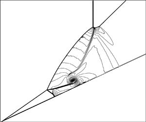
Case 3 lies in the type IV region of figure 16, and the numerical results are displayed in figure 20. An enlarged partial view of the Mach contours is given in figure 20(a). An enlarged partial view of pressure is displayed in figure 20(b). The global view of the pressure contours is displayed in figure 20(c). The streamlines marked in figure 20(c) are based in the frame co-moving with  $P$. The structure is the same as type IV shock interference as displayed in figure 12: it has two incident shock waves, a Mach stem and a jet.

Figure 20. Type IV shock interaction for  $\theta _{w}=10^{\circ }$,
  $M_{r}=6$,
  $M_{s}=5.498$: (a) Mach contours; (b) pressure contours; (c) global view of pressure contours.
3.4. Type I and type II shock interference due to flow deflection angle reversal
The line  $\theta _{w}=\theta _{CE}(M_{r},M_{s})$ in figure 16, which separates regions
  $C$ and
  $E$, is of particular interest. This line corresponds to
  $\Delta \theta =0$, where
  $\Delta \theta$, defined by (3.1), is the flow deflection angle across shock
  $S_{OR}$. Thus the line
  $\theta _{w}=\theta _{CE}(M_{r},M_{s})$ corresponds to the condition with flow deflection angle reversal discussed in § 3.2; see figure 14(a). Below this line, the shock
  $S_{OR}$, which is the downstream incident shock for type IV, V and VI shock interference when
  $\theta _{w}>\theta _{CE}(M_{r},M_{s})$, can no longer be regarded as an incident shock wave of the equivalent problem, but should be regarded as a reflected shock one. This means that the newly generated shock oblique shock wave
  $S_{NE}$ (see figure 3b) should be one incident shock wave, apart from the RMS (
 $I_{S}$). The shock
  $I_{S}$ and the shock
  $S_{NE}$ then constitute two incident shock waves of different families, which should have type I and type II shock interaction (Keyes & Hains Reference Keyes and Hains1973; Grasso et al. Reference Grasso, Purpura and Délery2003). The line
  $\theta _{w}=\theta _{EF}(M_{r},M_{s})$ in figure 16 is the transition condition between type I and type II shock interference. Region
  $E$ above
  $\theta _{w}=\theta _{EF}(M_{r},M_{s})$ should have type II shock interference, and region
  $F$ below
  $\theta _{w}=\theta _{EF}(M_{r},M_{s})$ should have type I shock interference.
Case 4 in table 1 lies in region  $E$, where we should have type II shock interference. The numerical solution for case 4 is displayed in figure 21, which is indeed type II shock interference. Figure 21(a) shows the Mach contours, figure 21(b) gives the pressure contours, and figure 21(c) shows the Mach contours and streamlines seen from the frame co-moving with the intersection point
  $P$. In this case, shock
  $S_{OR}$ is one reflected shock of the type II shock interference, and shock
  $I_{S}$ and the newly generated SOSW(
 $S_{NE}$) are the two incident shock waves according to the streamlines shown in figure 21(c). The shock
  $S_{R2}$ is the other reflected shock wave.

Figure 21. Type II shock interaction for  $\theta _{w}=5^{\circ }$,
  $M_{r}=6$,
  $M_{s}=5.498$: (a) Mach contours; (b) pressure contours; (c) Mach contours and streamlines in the co-moving frame.
Case 5 in table 1 lies in region  $F$, where we should have type I shock interference. The numerical solution for case 5 is displayed in figure 22, which is indeed type I shock interference. Figure 22(a) shows the Mach contours, figure 22(b) gives the pressure contours, and figure 22(c) shows the Mach contours and streamlines seen from the frame co-moving with the intersection point
  $P$ of
  $I_{S}$ and
  $S_{OR}$. In this case, shock
  $S_{OR}$ is one reflected shock of the type I shock interference, and shock
  $I_{S}$ and the newly generated SOSW(
 $S_{NE}$) are the two incident shock waves according to the streamlines shown in figure 22(c). The shock
  $S_{R2}$ is the other reflected shock wave.

Figure 22. Type I shock interaction for  $\theta _{w}=2^{\circ }$,
  $M_{r}=6$,
  $M_{s}=5.498$: (a) Mach contours; (b) pressure contours; (c) Mach contours and streamlines in the co-moving frame.
Note that type I and type II shock interactions are called regular reflection and Mach reflection in asymmetric shock reflections (Li et al. Reference Li, Chpoun and Ben-Dor1999; Ivanov et al. Reference Ivanov, Ben-Dor, Elperin, Kudryavtsev and Khotyanovsky2002).
4. Reflection types and transition conditions for an RMS of the second family
This section is divided into five subsections, devoted respectively to display of some shock reflection patterns (using CFD) including the subdivision of the global reflection structure into primary and secondary reflection structures, the method for transition analysis of primary reflection, the method for transition analysis of secondary reflection, and the transition conditions for various shock reflection patterns.
4.1. Some shock reflection patterns: primary and secondary reflections
As noted in § 1, shock reflection for an RMS of the second family has been studied before within the context of shock-on-shock interaction. Li & Ben-Dor (Reference Li and Ben-Dor1997) considered an oblique incident shock wave and derived analytical solutions for various shock reflection patterns. Law et al. (Reference Law, Felthun and Skews2003) performed some numerical simulation for shock-on-shock interaction, considering both oblique and normal incident shock waves. These studies have considered the influence of shock angle of the incident shock. Here, we study shock patterns and transition conditions for a normal shock, as for an RMS of the first family, with the emphasis on the role of shock speed. More subtypes of shock reflection patterns are expected to be found here.
Since the shock reflection patterns may be rather complex, it is convenient to consider the global reflection pattern to be a combination of primary reflection and secondary reflection. The primary reflection is the direct reflection at the intersection of the RMS ( $I_{S}$) and the SOSW (
 $S_{OR}$). It may produce regular reflection (RR) and Mach reflection (MR). The secondary reflection is the reflection of reflected shock waves from primary reflection. It may also produce regular reflection and Mach reflection; the latter will be called irregular reflection (IR) to follow the terminology in past studies of pseudo-steady reflection.
Three properly chosen test cases showing different primary shock reflection structures, with  $\theta _{w}$,
  $M_{s}$ and
  $M_{r}$ as given in table 2, are used for numerical simulation.
Table 2. Test cases for an RMS of the second family. The parameters  $\theta _{w}$,
  $M_{s}$ and
  $M_{r}$ are specified. The pressure ratio
  $p_{l}/p_{r}$ is computed by (2.10).

For case 1, the Mach contours at a typical instant are displayed in figure 23(a), and the reflection pattern, displaying the main flow structures and ignoring some details about interaction between shock waves and sliplines, is displayed in figure 23(b). The primary reflection, i.e. the direct reflection at the intersection of the RMS ( $I_{S}$) and the SOSW (
 $S_{OR}$), is a Mach reflection, with Mach stem
  $Tp_{1}Tp_{2}$. The secondary reflection of the lower reflected shock wave, reflected from the triple point
  $Tp_{2}$, is an irregular reflection on the wedge, which produces another triple point
  $Tp_{3}$. There is a kink (
 $K$) on the reflected shock wave from triple point
  $Tp_{1}$.

Figure 23. Shock reflection patterns for case 1: (a) Mach contours; (b) shock pattern.
For case 2, the Mach contours at a typical instant are displayed in figure 24(a), and the reflection pattern, with some details ignored, is displayed in figure 24(b). The primary reflection is a regular reflection. The secondary reflection of the lower reflected shock wave is an irregular reflection on the wedge, which produces another triple point  $Tp_{3}$. There is an additional triple point
  $Tp_{4}$ on the reflected shock from triple point
  $Tp_{1}$.

Figure 24. Shock reflection patterns for case 2: (a) Mach contours; (b) shock pattern.
For case 3, the Mach contours at a typical instant are displayed in figure 25(a) and the reflection pattern is displayed in figure 25(b). The primary reflection at point  $P$ is a regular reflection. The secondary reflection of the lower reflected shock wave produces a regular reflection at point
  $R$ on the wedge. The reflected shock from point
  $R$ further interacts with the slipline from the primary interaction point
  $P$, and this interaction produces a transmitted shock wave above that slipline. Similarly to case 2, there is an additional triple point
  $Tp_{4}$ on the reflected shock from the primary interaction point
  $P$. The reflected shock from
  $Tp_{4}$ will interact with the transmitted shock from
  $R$. The full details are not displayed here since in this study we are concerned mainly with the primary and secondary reflection structures.

Figure 25. Shock reflection patterns for case 3: (a) Mach contours; (b) shock pattern.
For an RMS of the second family, four possible primary–secondary reflection configurations, labelled RR-RR, RR-IR, MR-RR, MR-IR, are shown in figure 26. The RR-RR configuration (figure 26a) means that the RMS ( $I_{S}$) and the SOSW (
 $S_{OR}$) have regular reflection at their direct intersection point (
 $P$), and the reflected shock (
 $R_{S2}$) of this reflection has regular reflection on the wall (at point
  $R$). The RR-IR configuration (figure 26b) means that the RMS (
 $I_{S}$) and the SOSW (
 $S_{OR}$) still have regular reflection at their direct intersection point (
 $P$) , and the reflected shock (
 $R_{S2}$) of this reflection has irregular reflection on the wall (with its Mach stem at point
  $N$ on the wall). The MR-RR configuration (figure 26c) means that the RMS (
 $I_{S}$) and the SOSW (
 $S_{OR}$) have Mach reflection (with Mach stem
  $Tp_{1}Tp_{2}$), and the reflected shock (
 $R_{S2}$) of this reflection has regular reflection on the wall (at point
  $R$). The MR-IR configuration (figure 26d) means that the RMS (
 $I_{S}$) and the SOSW (
 $S_{OR}$) also have Mach reflection (with Mach stem
  $Tp_{1}Tp_{2}$) , and the reflected shock (
 $R_{S2}$) of this reflection has irregular reflection on the wall (with its Mach stem at point
  $N$ on the wall). Types RR-RR and RR-IR have been predicted and found numerically before (cf. Li & Ben-Dor Reference Li and Ben-Dor1997; Law et al. Reference Law, Felthun and Skews2003). The MR-RR configuration is not observed in our numerical simulation, as will be further mentioned at the end of § 4.4. The MR-IR configuration shown in figure 23(a) is different from the case reported before. (Previous studies appear to have reported not an
  $R_{S2}$ that further produces Mach reflection on the wall, but a curved
  $R_{S2}$ directly connected to the wall, the condition for which will be studied in § 4.5.)

Figure 26. Possible flow patterns for an RMS of the second family. The reflection at the intersection point  $P$ is the primary reflection. The reflection of one reflected shock from primary reflection on the wedge is secondary reflection.
Apart from the secondary reflection of  $R_{S2}$ on the wall, the reflected shock
  $R_{S1}$ may also have secondary reflection structure; see § 4.5 for further discussion.
4.2. Method to find transition condition for primary reflection
The primary reflection, i.e. reflection between  $I_{S}$ and
  $S_{OR}$ at their intersection point (
 $P$), is an asymmetric reflection, and the reflection type can be decided in the frame co-moving with the intersection point
  $P$ of
  $I_{S}$ and
  $S_{OR}$, through looking for the von Neumann criterion and detachment criterion as by Li et al. (Reference Li, Chpoun and Ben-Dor1999) and Ivanov et al. (Reference Ivanov, Ben-Dor, Elperin, Kudryavtsev and Khotyanovsky2002) for steady asymmetric reflection. The flow parameters that need to be used for deriving the transition conditions are displayed in figure 27. We will use the superscript
  $(P)$ for flow parameters in the frame co-moving with the intersection point
  $P$.
$P$.

Figure 27. Schematic illustration of the asymmetric shock reflection in the co-moving frame with intersection point  $P$ (case RR-RR).
The flow velocity of region (0) in figure 27 is
 \begin{equation} (u_{0}^{(P)},v_{0}^{(P)})=(u_{r}-u_{P},-v_{P})=((M_{r}-M_{s})a_{r},-M_{s} a_{r}\tan \beta_{w}), \end{equation}
where  $(u_{P},v_{P})$, the velocity of the intersection point
  $P$, is given by (2.1). Putting (4.1) into
  $M_{0}^{(P)}=\sqrt {(u_{0}^{(P)})^{2} +(v_{0}^{(P)})^{2}}/a_{r}$ and
  $\theta _{0}^{(P)}=\arctan |{v_{0}^{(P)}/} {u_{0}^{(P)}}|$, and using (2.1), we get the following expressions for the Mach number and flow angle in region (0):
 \begin{equation} \left. \begin{aligned} M_{0}^{(P)} & =\sqrt{(M_{r}-M_{s})^{2}+(M_{s}\tan \beta_{w})^{2}},\\ \theta_{0}^{(P)} & =\arctan\left(\frac{M_{s}\tan \beta_{w}}{M_{s}-M_{r}}\right). \end{aligned} \right\} \end{equation}
The shock angles  $\beta _{1}^{(P)}$ and
  $\beta _{2}^{(P)}$ for the shocks
  $I_{S}$ and
  $S_{OR}$ in the frame co-moving with
  $P$ are related to
  $(u_{0} ^{(P)},v_{0}^{(P)})$ by
 \begin{equation} \left. \begin{aligned} & \beta_{1}^{(P)}=\arccos \left( \frac{|v_{0}^{(P)}|}{|(u_{0}^{(P)},v_{0} ^{(P)})|}\right),\\ & \beta_{2}^{(P)}=\arccos \left( \frac{|u_{0}^{(P)}\cos \beta_{w}+v_{0}^{(P)} \sin \beta_{w}|}{|(u_{0}^{(P)},v_{0}^{(P)})|}\right). \end{aligned} \right\} \end{equation}
 The expressions (4.2) and (4.3) provide the input parameters  $M_{0}^{{(P)}}$,
  $\theta _{0}^{{(P)}}$,
  $\beta _{1}^{{(P)}}$ and
  $\beta _{2}^{{(P)}}$ to be used for deriving the von Neumann condition and detachment condition using the method to find the transition condition of steady asymmetric reflection. In this paper, the shock waves
  $I_{S}$ and
  $S_{OR}$ are assumed to be weak shock waves viewing from the co-moving frame with point
  $P$. The case that they are strong shock waves is not considered.
The flow deflection angles  $\theta _{1}^{(P)}$ and
  $\theta _{2}^{(P)}$ across the shocks
  $I_{S}$ and
  $S_{OR}$ shown in figure 27 are obtained from
 \begin{equation} \tan{{\theta}_{k}^{(P)}}={{f}_{{{\theta}}}}(M_{0}^{(P)},\beta_{k} ^{(P)}),\quad k=1,2\text{ (weak solution)}, \end{equation}
and the Mach number and pressure in regions (1) and (2) are computed as
 \begin{equation} (M_{k}^{(P)})^{2}=f_{M}(M_{0}^{(P)},\beta_{k}^{(P)}), \quad p_{k}^{(P)} =p_{r}\,{f_{p}}(M_{0}^{(P)},\beta_{k}^{(P)}),\quad k=1,2. \end{equation}
 Referring to figure 27 for notations for shock angles and flow deflection angles, the pressures  ${p_{3}^{(P)}}$ and
  ${p_{4}^{(P)}}$ downstream of the reflected shock waves are computed by
 \begin{equation} \left. \begin{aligned} & \tan{\theta_{13}^{(P)}}={{f}_{{{\theta}}}}(M_{1}^{(P)},\beta_{13}^{(P)}),\quad{p_{3}^{(P)}}={p_{1}^{(P)}\,{f}_{p}}(M_{1}^{(P)},\beta_{13}^{(P)}),\\ & \tan{\theta_{24}^{(P)}}={{f}_{{{\theta}}}}(M_{2}^{(P)},\beta_{24} ^{(P)}),\quad{p_{4}^{(P)}}={p_{2}^{(P)}\,{f}_{p}}(M_{2}^{(P)},\beta_{24}^{(P)}). \end{aligned} \right\} \end{equation}
The expressions in (4.6) are solved along with the flow parallel condition
 \begin{equation} \left. \begin{aligned} & {\theta_{13}^{(P)}={\theta}_{1}^{(P)}-\theta}_{s}^{(P)},\\ & {\theta_{24}^{(P)}={\theta}_{2}^{(P)}+\theta}_{s}^{(P)}, \end{aligned} \right\} \end{equation}
and pressure balance condition
 \begin{equation} {p_{3}^{(P)}=p_{4}^{(P)}}. \end{equation}
In (4.7),  ${\theta }_{s}^{(P)}$ is the slipline angle as shown in figure 27, and is assumed positive if it deflects in the anticlockwise direction relative to the direction of
  $(u_{0}^{(P)} ,v_{0}^{(P)})$.
For given  $M_{r}$ and
  $M_{s}$, the detachment condition
  ${{\theta }_{w}}= \theta _{w}^{(D)}(M_{r},{M_{s}})$ is the condition of
  ${{\theta }}_{w}$ at which either
  ${\theta _{13}^{(P)}}$ reaches its detached angle or
  ${\theta _{24}^{(P)}}$ reaches its detached angle, i.e.
 \begin{equation} {\theta_{13}^{(P)}=\theta}_{max}{(M_{1}^{(P)})}\quad\text{or}\quad{\theta_{24} ^{(P)}=\theta}_{max}{(M_{2}^{(P)})}. \end{equation}
See (2.5) for the expression for the detached angle.
For given  $M_{r}$ and
  $M_{s}$, the von Neumann condition
  ${{\theta }_{w}}=\theta _{w}^{(N)}(M_{r},{M_{s}})$ is the condition of
  ${{\theta }}_{w}$ at which
 \begin{equation} {p_{m}^{(P)}}={p_{3}^{(P)}}\quad\text{or}\quad{p_{m}^{(P)}}={p_{4}^{(P)}}, \end{equation}
where the pressure  ${p_{m}^{(P)}}$ downstream of a strong shock wave with flow deflection angle
  ${\theta }_{s}^{(P)}$ and with the upstream Mach number
  $M_{0}^{(P)}$ is calculated from
 \begin{equation} {p_{m}^{(P)}}={{p}}_{r}\left( 1+\frac{2\gamma}{\gamma+1}\left( {{\left( M_{0}^{(P)}\sin \beta_{s}^{(P)}\right) }^{2}}-1\right) \right), \end{equation}
with  $\beta _{s}^{(P)}$ being the strong shock wave solution of
  $\tan {\theta }_{s}^{(P)}=f_{\theta}(M_{0}^{(P)},\beta _{s}^{(P)})$.
4.3. Method for transition condition of secondary reflection of  $R_{S2}$

The secondary reflection, i.e. reflection of the reflected shock  $R_{S2}$ on the wedge, at point
  $R$ as shown in figure 26, is a pseudo-steady reflection similar to that shown in figures 1(c,d). To find the transition condition of such a reflection, we need to know the velocity of
  $R_{S2}$. For RR-IR and RR-RR as shown in figure 26, this velocity can be found easily, and the transition condition will be considered in this subsection. For MR-IR and MR-RR in figure 26 this velocity can not be found easily.
Now consider pseudo-steady reflection of  $R_{S2}$ on the wedge. In a conventional study of pseudo-steady reflection, as shown in figures 1(c,d), the incident shock is in a vertical direction, i.e. the angle
  $\beta _{R}$ displayed in figure 27 satisfies
  $\beta _{R}+\theta _{w}=90^{\circ }$. Here it satisfies
 \begin{equation} \beta_{R}=\theta_{0}^{(P)}-\theta_{2}^{(P)}+\beta_{24}^{(P)}-\theta_{w}. \end{equation}
 To find the transition condition, we need the speed  $V_{R}$ of the intersection point
  $R$ between
  $R_{S2}$ and the wedge surface. Note that
  $R$ moves along the surface of the wedge. The flow parameters used for this are displayed schematically in figure 28, from which it can be seen that the following geometrical relation holds:
 \begin{equation} \frac{RA}{\sin \omega}=\frac{PA}{\sin \beta_{R}}, \end{equation}
with  $\omega =\beta _{R}-(\beta _{w}-\theta _{w})$. The speed of
  $R$ is related to the speed
  $V_{P}$ of point
  $P$ by
  $V_{R}=V_{P}({RA}/{PA})$, where
  $V_{P}=M_{s}a_{r}/\cos (\beta _{w})$ is the modulus of
  $\boldsymbol {V}_{P}$ already given by (2.1). Using (4.13) for
  ${RA}/{PA}$, we get
 \begin{equation} V_{R}=\frac{\sin(\beta_{R}-(\beta_{w}-\theta_{w}))}{\cos(\beta_{w})\sin (\beta_{R})}\,M_{s}a_{r}. \end{equation}
Figure 28. Flow parameters for determining the velocity of  $R$.
$R$.
Now we use superscript  $(R)$ to denote flow parameters in the frame co-moving with
  $R$. The Mach number
  $M_{d}^{(R)}$ in region
  $(d)$ is thus
 \begin{equation} M_{d}^{(R)}=\frac{V_{R}}{a_{d}}-M_{d}, \end{equation}
where  $M_{d}$ is the ground frame Mach number in region
  $(d)$ calculated by
  $M_{d}^{2}=f_{M}(M_{r},\beta _{w})$, and
  $a_{d}$ is the sound speed in region
  $(d)$ that follows from the sound speed expression and the oblique shock wave relation for density and pressure.
Now, with  $M_{d}^{(R)}$ and
  $\beta _{R}$ determined, the transition condition between RR and IR at point
  $R$ can be decided as for pseudo-steady reflection. Out of various suggested criteria for the termination of RR, Ben-Dor (Reference Ben-Dor2006) pointed out that the one that best agrees with pseudo-steady shock tube experimental data is from the length scale concept of Hornung et al. (Reference Hornung, Oertel and Sandeman1979). This concept suggests that in pseudo-steady flows, RR terminates when the flow behind the reflection point,
  $R$, of the RR becomes sonic in a frame co-moving with
  $R$. With
  $M_{k}^{(R)}$ (
 $k=1,2$) denoting the Mach number in region
  $(k)$ (
 $k=1,2$) of figure 28(a) in the frame co-moving with
  $R$, this criterion implies that the transition occurs when
 \begin{equation} M_{2}^{(R)}=1, \end{equation}
where  $M_{2}^{(R)}$ can be derived from the oblique shock wave relations
 \begin{equation} (M_{2}^{(R)})^{2}={f_{M}}(M_{1}^{(R)},\beta_{12}^{(R)}), \end{equation}
where  $M_{1}^{(R)}$ is calculated from
  $(M_{1}^{(R)})^{2}={f_{M}}(M_{d} ^{(R)},\beta _{R})$, and
  $\beta _{12}^{(R)}$ is the weak solution of
  $\tan {{\theta }_{d1}^{(P)}}={{f}_{{{\theta }}}}(M_{1}^{(R)},\beta _{12}^{(R)})$, with
  ${{\theta }_{d1}^{(P)}}$ determined by
  $\tan {{\theta }_{d1}^{(P)}} ={{f}_{{{\theta }}}}(M_{d}^{(R)},\beta _{R})$.
4.4. Transition conditions in the $M_{s}-\theta _{w}$ and $M_{r} -\theta _{w}$ planes


The transition conditions are expressed in either the  $M_{s}$–
 $\theta _{w}$ plane for fixed
  $M_{r}$, or the
  $M_{r}$–
 $\theta _{w}$ plane for fixed
  $M_{s}$. The transition conditions in the
  $M_{s}$–
 $\theta _{w}$ plane for
  $M_{r}=5$ are displayed in figure 29(a), and the transition conditions in the
  $M_{r}$–
 $\theta _{w}$ plane for
  $M_{s}=10$ are displayed in figure 29(b). The shock polars for primary reflection in three cases (cases 1 and 2 shown in figure 29(a), and case 3 in figure 29(b) – see also table 2) are displayed in figure 30, with the
  $I$ polar obtained from inflow Mach number
  $M_{0}^{(P)}$, and the
  $R_{1}$ and
  $R_{2}$ polars obtained from shock deflection angles
  $\theta _{1}^{(P)}$ and
  $\theta _{2}^{(P)}$.

Figure 29. Transition criteria: (a) in the  $M_{s}$–
 $\theta _{w}$ plane for
  $M_{r}=5$; (b) in the
  $M_{r}$–
 $\theta _{w}$ plane for
  $M_{s}=10$.

Figure 30. Shock polars for the primary reflection (in the frame co-moving with  $P$): (a) case 1; (b) case 2; (c) case 3.
In figure 29(a), the range of  $M_{s}$ is
  $M_{s}\in \lbrack 6.1,32]$. In figure 29(b), the range of
  $M_{r}$ is
  $M_{r}\in \lbrack 2,8.9]$. This range is chosen from the requirement that
  $M_{s}>M_{r}+1$ for an RMS of the second family.
Regions with RR, double solution (DSD) and MR shown in figure 29 are reflection types for primary reflection. Inside region  $C$ (Mach reflection), the line
  $\theta _{w}=\theta _{min}(M_{r},M_{s})$ is the critical angle to have one or more strong incident shock wave in the co-moving frame of the intersection point
  $P$ of
  $I_{s}$ and
  $S_{OR}$. The flow pattern below
  $\theta _{w}=\theta _{min}(M_{r},M_{s})$ will be discussed further in § 4.5. The dual solution domain is bounded below by the von Neumann criterion
  ${{\theta }_{w}}=\theta _{w}^{(N)}(M_{r},{M_{s}})$ computed by (4.10), and bounded above by the detachment criterion
  ${{\theta }_{w}}=\theta _{w}^{(D)}(M_{r},{M_{s}})$ computed by (4.9). It is interesting to note that regular reflection occurs for large
  $\theta _{w}$, while MR occurs for small
  $\theta _{w}$, which appears to be counter-intuitive. A similar phenomenon is observed for an RMS of the first family, where type IV shock interference occurs at smaller
  $\theta _{w}$ while type VI shock interference occurs at larger
  $\theta _{w}$.
The line  ${{\theta }_{w}}=\theta _{RR,IR}(M_{r},{M_{s}})$ in figure 29 is the critical condition for transition of secondary reflection, i.e. for transition of the reflected shock wave
  $R_{S2}$ over the wedge, in a region where the primary reflection is a regular reflection. On the left-hand side of
  ${{\theta }_{w}}=\theta _{RR,IR}(M_{r},{M_{s}})$, we have RR-IR. On the right-hand side of
  ${{\theta }_{w}}=\theta _{RR,IR}(M_{r},{M_{s}})$, we have RR-RR. In a region where the primary reflection is a Mach reflection, there is no simple way to obtain a similar transition criterion for the secondary reflection, since the velocity of the triple point
  $Tp_{2}$ is not known. As stated in § 4.1, the MR-RR configuration (figure 26c) did not appear in our numerical simulation. Since there is no simple way to derive the velocity of triple point
  $Tp_{2}$, no conclusion can be drawn about whether MR-RR is possible.
Now let us return to the shock polars displayed in figure 30. For case 1, the  $R_{1}$ and
  $R_{2}$ polars have no intersection so the reflection type is MR. For case 2, the
  $R_{1}$ and
  $R_{2}$ polars have an intersection that is above the other two intersection points (the intersection point of the
  $R_{1}$ and
  $I$ polars, and the intersection point of the
  $R_{2}$ and
  $I$ polars), which means that case 2 is in the DSD domain. For case 3, the intersection point of the
  $R_{1}$ and
  $R_{2}$ polars is below the other two intersection points (the intersection point of the
  $R_{1}$ and
  $I$ polars, and the intersection point of the
  $R_{2}$ and
  $I$ polars), so the reflection type for case 3 is RR.
For another set of conditions, the results are similar. For instance, figure 31(a) presents the transition conditions in the  $M_{r}$–
 $\theta _{w}$ plane with
  $M_{s}=20$. It can be seen that the transition criteria are similar to those shown in figure 29(b) for
  $M_{s}=10$. It is interesting to note that there is a non-monotonic variation for the detachment condition especially after
  $M_{r}\approx 17$. This non-monotonicity is made evident through displaying, in figure 31(b), the shock polars at points 1, 2 and 3 (with different
  $M_{r}$ but with
  $\theta _{w}=10.3^{\circ }$,
  $M_{s}=20$) from figure 31(a). We observe MR for point 1, DSD for point 2, and MR again for point 3.

Figure 31. (a) Transition criteria for  $M_{s}=20$. (b) Shock polars (for points 1, 2 and 3).
The non-monotonicity might be due to the combined effects of the variations of the equivalent flow parameters ( $M_{0}^{(p)}$,
  $\beta _{1}^{(P)}$ and
  $\beta _{2}^{(P)}$, computed by (4.2) and (4.3)) with respect to
  $M_{r}$, and these variations are shown in figure 32.

Figure 32. Dependence of some equivalent flow parameters on  $M_{r}$ for
  $M_{s}=20$: (a) equivalent Mach number
  $M_{0}^{(P)}$; (b) equivalent shock angles
  $\beta _{1}^{(P)}$ and
  $\beta _{2}^{(P)}$.
4.5. Brief discussion of refection of secondary shock waves $R_{S1}$ and $R_{S2}$


The reflection of the secondary shock waves  $R_{S1}$ and
  $R_{S2}$ shown in figure 26 may involve more patterns than discussed above. However, a complete study of all the possibilities is beyond the scope of this paper. Here we simply make an incomplete discussion.
4.5.1. Reflection of the secondary shock wave $R_{S1}$

In conventional pseudo-steady shock reflection, where a moving shock wave reflects over a wedge immersed initially in a still gas (as shown in figure 1d), the reflected shock wave (like  $R_{S1}$ here) in the case of Mach reflection may be smooth (a situation called single Mach reflection, SMR), have a kink (a situation called transitional Mach reflection, TMR), or have a new triple point (a situation called double Mach reflection, DMR); see figures 12 and 22 of Ben-Dor (Reference Ben-Dor2006) for more detailed classification of subtypes (such as direct, stationary, inverse Mach reflections, DMR
 $+$, DMR
 $-$, or terminated RR) and transition conditions between various types of shock reflection.
It would be possible that for the present problem, the reflected shock wave  $R_{S1}$ from point
  $Tp_{1}$ of figure 23(b), or point
  $P$ of figures 24(b) and 25(b), may also have a kink (point
  $K$) or an additional triple point. Indeed, in case 1 (MR-IR), we observe a kink according to figure 23(a), and this kink is marked
  $K$ in figure 23(b). In this case, the primary reflection may be regarded as transitional Mach reflection. Previous studies (cf. Li & Ben-Dor Reference Li and Ben-Dor1997; Law et al. Reference Law, Felthun and Skews2003) showed cases not with such a kink, but with a smooth
  $R_{S1}$. Now we also show a case with a smooth
  $R_{S1}$. This case has
  $M_{s}=20$,
  $M_{r}=8$,
  $\theta _{w}=5^{\circ }$, corresponding to point 4 in figure 31(a), and this point is in the region below
  $\theta _{w}=\theta _{min }(M_{r},M_{s})$ (below which the incident shock is strong). The Mach contours and pressure contours for this condition are displayed in figures 33(a,b), respectively. In this case,
  $R_{S1}$ is smooth and the primary reflection can be regarded as a single Mach reflection. However, we are unable to find a case for which the primary reflection (in the case of Mach reflection) is a double Mach reflection.

Figure 33. Shock reflection patterns for point 4 in figure 31(a) ( $M_{s}=20$,
  $M_{r}=8$,
  ${{\theta }_{w}=5}^{\circ }$): (a) Mach contours; (b) pressure contours.
The finding that we may have a smooth  $R_{S1}$ or a kink on
  $R_{S1}$ raises the issue of determining further transition criteria to distinguish the conditions for SMR, TMR or possibly DMR for the present problem. Since TMR is observed above
  $\theta _{w}=\theta _{min}(M_{r},M_{s})$, and SMR is observed below, one may wonder whether
  $\theta _{w}=\theta _{min}(M_{r},M_{s})$ is the transition condition between SMR and TMR. However, this requires further study since transition conditions between SMR, TMR and DMR are far more complex than this even in the conventional pseudo-steady shock reflection problem, according to the studies by Li & Ben-Dor (Reference Li and Ben-Dor1995) and Semenov et al. (Reference Semenov, Berezkina and Krassovskaya2012).
In the conventional pseudo-steady shock reflection problem, the entire reflection process was treated as a combination of the shock-reflection process and the flow-deflection process (Li & Ben-Dor Reference Li and Ben-Dor1995). The transition condition between TMR and DMR requires knowledge of the velocity of the kink or the additional triple point, and simplified models, as given in the appendices of Li & Ben-Dor (Reference Li and Ben-Dor1995), are already complex in the conventional pseudo-steady shock reflection case. If we follow the same approach, then the present problem is much more complicated since we need to know in addition the velocity of the triple point ( $Tp_{1}$) of figures 26(c,d). Li & Ben-Dor (Reference Li and Ben-Dor1997) provides a theory to estimate the velocity or trajectory in the equivalent shock-on-shock interaction problem. Thus, to derive transition conditions for various types of
  $R_{S1}$ following the same approach as Li & Ben-Dor (Reference Li and Ben-Dor1995) and Li & Ben-Dor (Reference Li and Ben-Dor1997), one would have to combine the triple point trajectory theory of Li & Ben-Dor (Reference Li and Ben-Dor1995) for a kink or a second triple point on
  $R_{S1}$, and the theory of Li & Ben-Dor (Reference Li and Ben-Dor1997) for the triple point
  $Tp1$ shown in figures 26(c,d). It appears that such an analytical study would be highly complex, if not impossible, if one wished to derive transition conditions for various possible types of
  $R_{S1}$, similar to that given in figure 10 of Li & Ben-Dor (Reference Li and Ben-Dor1995) for the conventional pseudo-steady problem. Such a study will thus not be considered in the present paper, but may be considered in the future.
4.5.2. Reflection of the secondary shock wave $R_{S2}$ on the wall

The reflection pattern of  $R_{S2}$ on the wall might also have more subtypes than shown in figure 26, if it were considered as the incident shock in the conventional pseudo-steady shock reflection problem. We immediately have the same difficulty as shown above for
  $R_{S1}$ if one wants to investigate more details about the possible flow structure and the transition conditions, so such an issue is not considered in this study. We simply consider the subcase when
  $R_{S1}$ becomes strong with respect to its reflection point on the wall.
The Mach contours displayed in figure 23(a) correspond to case 1 in figure 29(a), for which  $R_{S2}$ has Mach reflection, while the work of Li & Ben-Dor (Reference Li and Ben-Dor1997) and Law et al. (Reference Law, Felthun and Skews2003) shows only a curved
  $R_{S2}$. Here we examine under which conditions this might occur.
In figure 26,  $R_{S2}$ is considered as a weak shock. In fact,
  $R_{S2}$ may be also a strong shock wave seen from the reference frame attached to its intersection point on the wedge (point
  $R$ of figure 26), according to the critical line
  $\theta _{w}=\omega (M_{r} ,M_{s})$ shown in figures 34(a,b) (which are obtained when the primary reflection is RR), which use the same conditions as figures 29(b) and 31(a). The critical line
  $\theta _{w} =\omega (M_{r},M_{s})$ is the condition above which
  $R_{S2}$ is weak and below which
  $R_{S2}$ is strong, in the frame co-moving with point
  $R$ of figure 26. Shock reflection with
  $R_{S2}$ strong happened to be computed by Law et al. (Reference Law, Felthun and Skews2003), who used a reference frame in which both shock waves are moving. Using the present frame (attached to the wedge), their cases in their figure 13(a,c) correspond to
  $M_{s}=7.077$,
  $M_{r} =4.431$,
  ${{\theta }_{w}=6}^{\circ }$ (called case 1 here), and
  $M_{s}=7.077$,
  $M_{r} =4.431$,
  ${{\theta }_{w}=12}^{\circ }$ (called case 2 here). These two cases will be used for comparison here.

Figure 34. For primary reflection of RR, the region with  $R_{S2}$ being strong is displayed as the dashed region. Transition criteria in the
  $M_{r}$–
 $\theta _{w}$ plane for (a)
  $M_{s}=10$, (b)
  $M_{s}=20$.
For  $M_{s}=7.077$, the transition conditions, similar to those shown in figure 34, are displayed in figure 35(a). Figure 35(b) is the anticipated flow pattern. Cases 1 and 2 are shown as circles in figure 35(a). The mentioned two cases of Law et al. (Reference Law, Felthun and Skews2003) are indeed below the critical line
  $\theta _{w}=\omega (M_{r},M_{s})$, i.e.
  $R_{S2}$ is strong in the reference frame co-moving with
  $R$.
$R$.

Figure 35. Shock reflection with strong  $R_{S2}$: (a) transition criteria showing the critical line below which
  $R_{S2}$ is strong (for
  $M_{s}=7.077$); (b) hypothetical flow pattern (NR means no reflection).
The Mach contours for both cases computed here are displayed in figure 36(a,b). They compare well with numerical results of figure 13(a,c) of Law et al. (Reference Law, Felthun and Skews2003). The flow pattern in figure 36(a) is indeed similar to the anticipated flow pattern shown in figure 35(b).

Figure 36. (a) Mach contours for case 1 ( $M_{s}=7.077$,
  $M_{r}=4.431$,
  ${{\theta }_{w} =6}^{\circ }$). (b) Mach contours for case 2 (
 $M_{s}=7.077$,
  $M_{r}=4.431$,
  ${{\theta } _{w}=12}^{\circ }$).
Thus, at the condition well below the critical line  $\theta _{w}=\omega (M_{r},M_{s})$, we recover the shock reflection part of previous studies, for which the reflected shock
  $R_{S2}$ is a curved strong shock.
5. Conclusion
This paper addressed the reflection of a rightward moving shock (RMS) wave over a steady oblique shock wave (SOSW), the latter generated by a wedge immersed initially in a steady supersonic flow. Both families (the first and second families) are considered for the RMS wave. The shock patterns and transition conditions are studied.
For a rightward moving incident shock wave of the first family, we used a transformation to show that for a sufficiently large wedge angle, the original shock reflection problem can be switched to an equivalent steady shock interaction problem where the RMS and the right part of the SOSW are the two incident shock waves of the same family. Thus type VI, V, IV shock interactions may occur.
For a rightward moving incident shock wave of the first family reflecting over the steady shock produced by a wedge with a small wedge angle, a flow deflection angle reversal is observed, and the right part of the SOSW can no longer be regarded as one incident shock wave. Now the left part of the SOSW becomes one incident shock wave. This situation produces type I or type II shock interference.
For a rightward moving incident shock wave of the second family, studied previously within the context of shock-on-shock interaction, we decomposed the reflection into a combination of primary reflection (between the RMS and the SOSW) and secondary reflection (reflection of the reflected shock waves from primary reflection) and identified the transition conditions in the shock speed–wedge angle plane for major reflection phenomena. For secondary reflection, one reflected shock wave impinges the wall to create regular reflection (RR) or irregular reflection (IR), and the other reflected shock wave is similar to the reflected wave of the classic pseudo-steady shock reflection (i.e. pseudo-steady shock reflection by a moving shock wave off a wedge immersed initially in a still gas). This other reflected shock wave may be smooth, or have a kink or another triple point similar to single Mach reflection, transitional Mach reflection and double Mach reflection observed from the classical pseudo-steady shock reflection. Hence there are quite a number of combinations of shock reflection patterns, more than predicted before in shock-on-shock interaction studies. However, the critical conditions for transition between various possible shock patterns of secondary reflected shock waves need more study in the future.
The large number of shock reflection patterns and the complexity of transition between various reflection patterns revealed in this study for reflection of RMSs of the two families on an SOSW enrich our knowledge of shock reflection or shock interaction. In this paper, we mainly considered the primary reflection patterns and their transition conditions, with some details about the secondary reflection not fully considered. These details may be considered in future studies.
Acknowledgement
The authors wish to thank the Referees, whose comments and suggestions were very useful for improving the paper.
Funding
This work was supported partly by the National Key Project (Grant no. GJXM92579) and by the National Science and Technology Major Project 2017-II-003-0015.
Declaration of interests
The authors report no conflict of interest.
Appendix. Triple point structure identification (TPSI) method
When CFD gives numerical results from which one perceives a number of moving triple points, it is difficult to determine which shock waves are the incident one, reflected one and Mach stem, as illustrated in figure 8 for steady flow. The TPSI method proposed by Wang & Wu (Reference Wang and Wu2021) makes it easier to identify the nature of various shock waves connected to a numerically computed moving triple point.
The method is, in fact, simple. Pick up the velocity of the triple point, say  $\boldsymbol {V}_{TP}$, from numerical solutions at two different instants. The original flow velocity
  $\boldsymbol {V}$ by numerical computation is then subtracted from
  $\boldsymbol {V}_{TP}$ to get
  $\boldsymbol {V}^{(TP)}=\boldsymbol {V}-\boldsymbol {V}_{TP}$. We then use
  $\boldsymbol {V}^{(TP)}$ to draw the streamlines and Mach contours. This gives the streamlines and Mach contours in the frame co-moving with the triple point. We then rotate the frame in such a way that the local inflow streamlines are horizontal, until the flow structure is comparable to that shown in figure 8 and from which it is clear which shock waves are the incident one, reflected one and Mach stem.
Consider the triple point  $Tp_4$ in figure 24(b) (case 2 in table 2). Figure 37(a) displays the Mach contours and streamlines in the ground frame. Using the numerical results, we measured
  $\boldsymbol {V}_{Tp4}=(23a_{r},20.2a_{r})$. Figure 37(b) displays the Mach contours and streamlines in the frame co-moving with the triple point, i.e. using
  $\boldsymbol {V}^{(TP)}=\boldsymbol {V}-\boldsymbol {V}_{TP}$.

Figure 37. Illustration of identification of the shock structure of a moving triple point. (a) Original ground frame solution near triple point  $Tp_4$. (b) Solution in the frame co-moving with the triple point
  $Tp_4$. (c) Numerical solution in the rotated frame. (d) Flow structure with the incident shock, reflected shock and Mach stem pertinent to triple point
  $Tp_4$ identified in the original ground frame.
Figure 37(c) shows the results by rotation of figure 37(b) in such a way the inflow is horizontal. It is then clear from figure 37(c) which shocks are the incident one, reflected one and Mach stem, now marked in figure 37(c).
By correspondence between figures 37(a) and 37(c), the nature of shock waves pertinent to triple point  $Tp_{4}$ is identified, as shown now in figure 37(d), which gives the flow structure in the original ground frame.
Here we showed the details of determining only an upward triple point. The method is similar for a downward triple point.


