


1 Introduction
The deformation of flexible bodies subject to a transverse oscillatory flow has raised the attention of the scientific community for some time and with different motivations. The propulsive performances of deformable bodies depend on the flexibility of the structure (Lighthill Reference Lighthill1960, Reference Lighthill1971; Katz & Weihs Reference Katz and Weihs1978, Reference Katz and Weihs1979). More specifically, the dynamic coupling with the deformation resulting from the oscillatory forcing may trigger resonances or involve nonlinear effects of paramount importance (Alben Reference Alben2008; Michelin & Llewellyn Smith Reference Michelin and Llewellyn Smith2009; Ramananarivo, Godoy-Diana & Thiria Reference Ramananarivo, Godoy-Diana and Thiria2011; Paraz, Eloy & Schouveiler Reference Paraz, Eloy and Schouveiler2014; Paraz, Schouveiler & Eloy Reference Paraz, Schouveiler and Eloy2016; Piñeirua, Thiria & Godoy-Diana Reference Piñeirua, Thiria and Godoy-Diana2017). Similarly, flexible structures forced into a transverse motion within an axial flow may harvest energy from the fluid, and the nature of the deformation depending on the features of the forcing influences the efficiency of the process (Liu, Xiao & Cheng Reference Liu, Xiao and Cheng2013).
The transverse fluid loads are also responsible for internal stresses that may endanger the structural integrity. As a strategy for survival, large plants living in flow-dominated habitats are usually very flexible (Harder et al. Reference Harder, Speck, Hurd and Speck2004). Thanks to their ability to deform under the influence of the current, flexible structures are able to reduce their frontal area, reshape themselves in a more streamlined fashion, or even shelter in regions where the flow is slower. The work of Vogel (Reference Vogel1984) and Vogel (Reference Vogel1989) has highlighted that this instantaneous, passive and reversible change of shape leads to a significant reduction of the internal stresses in the flexible plants subjected to high velocity flows. Because of the alleged adaptive nature of these flow-induced deformations, Vogel (Reference Vogel1984) has suggested the use of the word ‘reconfiguration’ owing to the more positive overtone associated with this term. Thereafter, several authors have contributed to quantitatively evaluate the drag reduction due to elastic reconfiguration in steady currents on model systems (Alben, Shelley & Zhang Reference Alben, Shelley and Zhang2002, Reference Alben, Shelley and Zhang2004; Gosselin, de Langre & Machado-Almeida Reference Gosselin, de Langre and Machado-Almeida2010; Luhar & Nepf Reference Luhar and Nepf2011; Hassani, Mureithi & Gosselin Reference Hassani, Mureithi and Gosselin2016; Leclercq & de Langre Reference Leclercq and de Langre2016).
But the question arises of whether the benefits of flexibility would still prevail in an oscillatory flow such as that encountered by salt marsh vegetation, seagrasses, or macroalgae in the near-shore waves. Koehl (Reference Koehl1984) pointed out that the fluid acceleration forces in an oscillatory flow, proportional to the volume of the plant when the drag is only proportional to its frontal area, may be the dominant load that bulk organisms have to withstand (see also Denny, Daniel & Koehl Reference Denny, Daniel and Koehl1985). On the other hand, flexible organisms long enough to move significantly with the flow may endure less severe relative flow and possibly benefit from a reduction of the associated loads. But the displacement of the structure is also responsible for additional inertial loads, so the actual consequences of flexibility in an oscillatory flow may be strongly dependent on the nature of the dynamic response of the deformable structure. Different mechanical models have been proposed to replicate the motion of macroalgae under the action of waves. For instance, see Friedland & Denny (Reference Friedland and Denny1995) for fully submerged flexible plants, Utter & Denny (Reference Utter and Denny1996), Denny & Cowen (Reference Denny and Cowen1997) for algae larger than the water depth and Gaylord & Denny (Reference Gaylord and Denny1997) for stipitate kelps. But the question of how the dynamical response and the associated loads may change when the rigidity of the structure is varied was first addressed by Luhar & Nepf (Reference Luhar and Nepf2016). Their study suggests, based on experimental results, that the drag on deformable structures may be expressed as that on a rigid structure with an effective length corresponding to the part of the actual structure over which significant relative fluid motion occurs. A scaling of this effective length with the flexibility was provided, with the aim to provide a tool to account for the deformability of near-bed organisms in the models of wave-energy dissipation (see also Luhar, Infantes & Nepf Reference Luhar, Infantes and Nepf2017). But the work of Luhar & Nepf (Reference Luhar and Nepf2016) focuses on the specific case where the amplitude of the flow is at most of the order of the length of the structure. They do not investigate either the dynamic interactions (such as possible resonance effects) due to high frequency loading. Besides, for particular values of the parameters, Luhar & Nepf (Reference Luhar and Nepf2016) notice an increase of the drag compared to the rigid case that is still not fully understood.
In order to identify and understand the different mechanisms involved, a systematic analysis exploring the space of forcing parameters is therefore still required. In this paper, we intend to elucidate the nature of the dynamical response of such a cantilever structure depending on the amplitude and frequency of the oscillating cross-flow, in the ideal case of a uniform flow. Our approach is mostly based on numerical simulations using reduced-order force models, with experimental validation. Our goal is then to assess how the structural stresses vary compared to the rigid case, depending on the different dynamical regimes.
In § 2 we introduce the theoretical model and the numerical method we chose to reproduce the dynamics of the system. In § 3 we present an experimental set-up used for visualizing the actual deformation of blades in oscillatory forced motion and to validate the model. We then identify four different kinematic regimes for varying ranges of the forcing amplitude and frequency in § 4, before discussing the resulting flexibility-induced variations of the structural stress in § 5. Finally, § 6 extends the discussion to provide general findings and to comment on previous work.
2 Model
2.1 Theory
We consider a neutrally buoyant, cantilever beam of length
 $L$
, width
$L$
, width
 $W$
and thickness
$W$
and thickness
 $D$
, placed perpendicular to a uniform oscillatory flow of velocity
$D$
, placed perpendicular to a uniform oscillatory flow of velocity
 $\boldsymbol{U}(t)=A\unicode[STIX]{x1D6FA}\sin (\unicode[STIX]{x1D6FA}t)\boldsymbol{e}_{\boldsymbol{x}}$
in a fluid of density
$\boldsymbol{U}(t)=A\unicode[STIX]{x1D6FA}\sin (\unicode[STIX]{x1D6FA}t)\boldsymbol{e}_{\boldsymbol{x}}$
in a fluid of density
 $\unicode[STIX]{x1D70C}$
(see figure 1). The amplitude
$\unicode[STIX]{x1D70C}$
(see figure 1). The amplitude
 $A$
corresponds to the maximal horizontal excursion of the fluid particles over one cycle, while
$A$
corresponds to the maximal horizontal excursion of the fluid particles over one cycle, while
 $\unicode[STIX]{x1D6FA}$
is the angular frequency of the oscillations.
$\unicode[STIX]{x1D6FA}$
is the angular frequency of the oscillations.

Figure 1. (a) Side view of the bending structure. (b) Dimensions of the undeformed blade.
We assume the thickness of the plate is small compared to its width (
 $D\ll W$
) so that deflection under the effect of the flow is confined in the
$D\ll W$
) so that deflection under the effect of the flow is confined in the
 $xz$
-plane. We also assume the structure is slender (
$xz$
-plane. We also assume the structure is slender (
 $L\gg W$
) so we can model it as a two-dimensional inextensible Euler–Bernoulli beam of bending stiffness
$L\gg W$
) so we can model it as a two-dimensional inextensible Euler–Bernoulli beam of bending stiffness
 $EI$
and mass per unit length
$EI$
and mass per unit length
 $m$
(see Audoly & Pomeau Reference Audoly and Pomeau2010). The curvilinear coordinate
$m$
(see Audoly & Pomeau Reference Audoly and Pomeau2010). The curvilinear coordinate
 $s$
represents the distance from the clamped edge along the span, and we use the prime symbol
$s$
represents the distance from the clamped edge along the span, and we use the prime symbol
 $(\cdot )^{\prime }$
to denote differentiation with respect to
$(\cdot )^{\prime }$
to denote differentiation with respect to
 $s$
. Hereafter,
$s$
. Hereafter,
 $\unicode[STIX]{x1D703}$
is the local angle of the tangent
$\unicode[STIX]{x1D703}$
is the local angle of the tangent
 $\unicode[STIX]{x1D749}=\boldsymbol{r}^{\prime }$
with the vertical axis
$\unicode[STIX]{x1D749}=\boldsymbol{r}^{\prime }$
with the vertical axis
 $\boldsymbol{e}_{\boldsymbol{z}}$
, where
$\boldsymbol{e}_{\boldsymbol{z}}$
, where
 $\boldsymbol{r}=x(s,t)\boldsymbol{e}_{\boldsymbol{x}}+z(s,t)\boldsymbol{e}_{\boldsymbol{z}}$
is the position vector. Following Audoly & Pomeau (Reference Audoly and Pomeau2010), the dynamic equilibrium reads
$\boldsymbol{r}=x(s,t)\boldsymbol{e}_{\boldsymbol{x}}+z(s,t)\boldsymbol{e}_{\boldsymbol{z}}$
is the position vector. Following Audoly & Pomeau (Reference Audoly and Pomeau2010), the dynamic equilibrium reads
 $$\begin{eqnarray}m\ddot{\boldsymbol{r}}=\boldsymbol{F}^{\prime }+\boldsymbol{q},\end{eqnarray}$$
where
 $\boldsymbol{q}$
is the external load per unit length on the structure,
$\boldsymbol{q}$
is the external load per unit length on the structure,
 $\boldsymbol{F}=T\unicode[STIX]{x1D749}+Q\boldsymbol{n}$
is the internal force vector, with
$\boldsymbol{F}=T\unicode[STIX]{x1D749}+Q\boldsymbol{n}$
is the internal force vector, with
 $T$
the tension and
$T$
the tension and
 $Q$
the shear force and the overdot stands for time derivation. The internal bending moment
$Q$
the shear force and the overdot stands for time derivation. The internal bending moment
 $M$
is related to the local curvature
$M$
is related to the local curvature
 $\unicode[STIX]{x1D705}=\unicode[STIX]{x1D703}^{\prime }$
by
$\unicode[STIX]{x1D705}=\unicode[STIX]{x1D703}^{\prime }$
by
 $M=EI\unicode[STIX]{x1D705}$
, and the shear force
$M=EI\unicode[STIX]{x1D705}$
, and the shear force
 $Q$
is given by
$Q$
is given by
 $Q=-M^{\prime }=-EI\unicode[STIX]{x1D705}^{\prime }$
. Clamping implies
$Q=-M^{\prime }=-EI\unicode[STIX]{x1D705}^{\prime }$
. Clamping implies
 $x=z=\unicode[STIX]{x1D703}=0$
at
$x=z=\unicode[STIX]{x1D703}=0$
at
 $s=0$
, while the free tip condition reads
$s=0$
, while the free tip condition reads
 $T=M=Q=0$
at
$T=M=Q=0$
at
 $s=L$
.
$s=L$
.
Because the structure is neutrally buoyant, its density is also
 $\unicode[STIX]{x1D70C}$
and gravity and buoyancy forces cancel each other. We assume large Reynolds number so that friction forces are negligible. Following Eloy, Kofman & Schouveiler (Reference Eloy, Kofman and Schouveiler2012), Singh, Michelin & de Langre (Reference Singh, Michelin and de Langre2012), Michelin & Doaré (Reference Michelin and Doaré2013), Piñeirua et al. (Reference Piñeirua, Thiria and Godoy-Diana2017) we model the effect of the relative flow as a combination of two external loads distributed along the span. First, the resistive drag (Taylor Reference Taylor1952)
$\unicode[STIX]{x1D70C}$
and gravity and buoyancy forces cancel each other. We assume large Reynolds number so that friction forces are negligible. Following Eloy, Kofman & Schouveiler (Reference Eloy, Kofman and Schouveiler2012), Singh, Michelin & de Langre (Reference Singh, Michelin and de Langre2012), Michelin & Doaré (Reference Michelin and Doaré2013), Piñeirua et al. (Reference Piñeirua, Thiria and Godoy-Diana2017) we model the effect of the relative flow as a combination of two external loads distributed along the span. First, the resistive drag (Taylor Reference Taylor1952)
 $$\begin{eqnarray}\boldsymbol{q}_{\boldsymbol{d}}=-1/2\unicode[STIX]{x1D70C}C_{D}W|U_{n}|U_{n}\boldsymbol{n}\end{eqnarray}$$
due to the pressure in the wake is purely normal. It is proportional to the square of the normal component
 $U_{n}$
of the relative velocity
$U_{n}$
of the relative velocity
 $\boldsymbol{U}_{\boldsymbol{r}}=U_{\unicode[STIX]{x1D70F}}\unicode[STIX]{x1D749}+U_{n}\boldsymbol{n}=\dot{\boldsymbol{r}}-\boldsymbol{U}$
. The drag coefficient
$\boldsymbol{U}_{\boldsymbol{r}}=U_{\unicode[STIX]{x1D70F}}\unicode[STIX]{x1D749}+U_{n}\boldsymbol{n}=\dot{\boldsymbol{r}}-\boldsymbol{U}$
. The drag coefficient
 $C_{D}$
depends on the geometry of the cross-section and is typically of order
$C_{D}$
depends on the geometry of the cross-section and is typically of order
 $O(1)$
. In pure sinusoidal flow, it slightly varies with the frequency through the Keulegan–Carpenter number
$O(1)$
. In pure sinusoidal flow, it slightly varies with the frequency through the Keulegan–Carpenter number
 $K_{C}=U/Wf=2\unicode[STIX]{x03C0}A/W$
(Keulegan & Carpenter Reference Keulegan and Carpenter1958). But in the case of a deformable body, the relative flow varies along the span and is not purely sinusoidal because of the motion of the structure itself. The exact value of
$K_{C}=U/Wf=2\unicode[STIX]{x03C0}A/W$
(Keulegan & Carpenter Reference Keulegan and Carpenter1958). But in the case of a deformable body, the relative flow varies along the span and is not purely sinusoidal because of the motion of the structure itself. The exact value of
 $C_{D}$
is however not critical here so we will simply use the value for steady flows. We will also assume a rectangular cross-section so we will use
$C_{D}$
is however not critical here so we will simply use the value for steady flows. We will also assume a rectangular cross-section so we will use
 $C_{D}=2$
. The second force component is the reactive (or added mass) force (Lighthill Reference Lighthill1971; Candelier, Boyer & Leroyer Reference Candelier, Boyer and Leroyer2011)
$C_{D}=2$
. The second force component is the reactive (or added mass) force (Lighthill Reference Lighthill1971; Candelier, Boyer & Leroyer Reference Candelier, Boyer and Leroyer2011)
 $$\begin{eqnarray}\boldsymbol{q}_{\boldsymbol{a}\boldsymbol{m}}=-m_{a}\left[\unicode[STIX]{x2202}_{t}(U_{n}\boldsymbol{n})-\unicode[STIX]{x2202}_{s}(U_{n}U_{\unicode[STIX]{x1D70F}}\boldsymbol{n})+{\textstyle \frac{1}{2}}\unicode[STIX]{x2202}_{s}(U_{n}^{2}\unicode[STIX]{x1D749})\right],\end{eqnarray}$$
where the added mass is given by
 $m_{a}=\unicode[STIX]{x1D70C}\unicode[STIX]{x03C0}W^{2}/4$
. This expression involves the normal component but also the tangential component
$m_{a}=\unicode[STIX]{x1D70C}\unicode[STIX]{x03C0}W^{2}/4$
. This expression involves the normal component but also the tangential component
 $U_{\unicode[STIX]{x1D70F}}$
of the relative velocity. In the case of an inextensible beam, this force becomes purely normal and its expression may be simplified in
$U_{\unicode[STIX]{x1D70F}}$
of the relative velocity. In the case of an inextensible beam, this force becomes purely normal and its expression may be simplified in
 $$\begin{eqnarray}\boldsymbol{q}_{\boldsymbol{a}\boldsymbol{m}}=-m_{a}\left[(\ddot{\boldsymbol{r}}-\dot{\boldsymbol{U}})\boldsymbol{\cdot }\boldsymbol{n}-2\dot{\unicode[STIX]{x1D703}}U_{\unicode[STIX]{x1D70F}}+\unicode[STIX]{x1D705}\left(U_{\unicode[STIX]{x1D70F}}^{2}-{\textstyle \frac{1}{2}}U_{n}^{2}\right)\right]\boldsymbol{n}.\end{eqnarray}$$
Finally, because the fluid itself is accelerated, a third force component has to be considered, called the virtual buoyancy force (Blevins Reference Blevins1990)
 $$\begin{eqnarray}\boldsymbol{q}_{\boldsymbol{v}\boldsymbol{b}}=m_{d}\dot{\boldsymbol{U}}.\end{eqnarray}$$
This term is due to the pressure gradient induced by the acceleration of the fluid. It is equivalent to the Archimedes force, only the acceleration of gravity is replaced by the acceleration of the fluid. It is proportional to the displaced mass per unit length
 $m_{d}=\unicode[STIX]{x1D70C}WD$
. We have assumed so far that the structure is fixed in an oscillating fluid. If the clamped edge of the structure was set into a forced horizontal motion of velocity
$m_{d}=\unicode[STIX]{x1D70C}WD$
. We have assumed so far that the structure is fixed in an oscillating fluid. If the clamped edge of the structure was set into a forced horizontal motion of velocity
 $\boldsymbol{U}_{\boldsymbol{f}}=U_{f}\boldsymbol{e}_{\boldsymbol{x}}$
, then the equilibrium equation in the frame of the structure (2.1) would include an additional load due to the inertial pseudo-force
$\boldsymbol{U}_{\boldsymbol{f}}=U_{f}\boldsymbol{e}_{\boldsymbol{x}}$
, then the equilibrium equation in the frame of the structure (2.1) would include an additional load due to the inertial pseudo-force
 $\boldsymbol{q}_{\boldsymbol{i}}=-m\dot{\boldsymbol{U}_{f}}$
. For a neutrally buoyant structure the displaced mass is equal to the structural mass (
$\boldsymbol{q}_{\boldsymbol{i}}=-m\dot{\boldsymbol{U}_{f}}$
. For a neutrally buoyant structure the displaced mass is equal to the structural mass (
 $m_{d}=m$
), so this inertial force has the same expression as the virtual buoyancy term (2.5) if
$m_{d}=m$
), so this inertial force has the same expression as the virtual buoyancy term (2.5) if
 $U_{f}=-U$
. Thus, oscillating a plate in a still fluid is actually equivalent to having a fixed structure in an oscillating flow, providing that the structure has the same density as the fluid. For practical reasons, in the experiments of § 3, we set the structure into motion rather than the fluid.
$U_{f}=-U$
. Thus, oscillating a plate in a still fluid is actually equivalent to having a fixed structure in an oscillating flow, providing that the structure has the same density as the fluid. For practical reasons, in the experiments of § 3, we set the structure into motion rather than the fluid.
In the following, we will only consider very thin blades
 $D\ll W$
(equivalently
$D\ll W$
(equivalently
 $m=m_{d}\ll m_{a}$
) so that we may neglect the structural inertia and the virtual buoyancy. The dynamic equilibrium (2.1) then reads
$m=m_{d}\ll m_{a}$
) so that we may neglect the structural inertia and the virtual buoyancy. The dynamic equilibrium (2.1) then reads
 $$\begin{eqnarray}\left[T+{\textstyle \frac{1}{2}}EI\unicode[STIX]{x1D705}^{2}\right]^{\prime }\unicode[STIX]{x1D749}+[\unicode[STIX]{x1D705}T-EI\unicode[STIX]{x1D705}^{\prime \prime }]\boldsymbol{n}+\boldsymbol{q}_{\boldsymbol{ d}}+\boldsymbol{q}_{\boldsymbol{a}\boldsymbol{m}}=0.\end{eqnarray}$$
After projection on the tangential and normal directions and elimination of the unknown tension
 $T$
, we finally obtain a single differential equation for the kinematic variables
$T$
, we finally obtain a single differential equation for the kinematic variables
 $\unicode[STIX]{x1D705}$
,
$\unicode[STIX]{x1D705}$
,
 $\unicode[STIX]{x1D703}$
,
$\unicode[STIX]{x1D703}$
,
 $\boldsymbol{r}$
 $$\begin{eqnarray}\displaystyle & & \displaystyle EI\left[\unicode[STIX]{x1D705}^{\prime \prime }+{\textstyle \frac{1}{2}}\unicode[STIX]{x1D705}^{3}\right]+{\textstyle \frac{1}{2}}\unicode[STIX]{x1D70C}C_{D}W|U_{n}|U_{n}\nonumber\\ \displaystyle & & \displaystyle \quad +\,m_{a}\left[\ddot{\boldsymbol{r}}\boldsymbol{\cdot }\boldsymbol{n}+\unicode[STIX]{x1D705}\left(U_{\unicode[STIX]{x1D70F}}^{2}-{\textstyle \frac{1}{2}}U_{n}^{2}\right)-2\dot{\unicode[STIX]{x1D703}}U_{\unicode[STIX]{x1D70F}}-\unicode[STIX]{x1D6FA}^{2}A\cos \unicode[STIX]{x1D703}\cos (\unicode[STIX]{x1D6FA}t)\right]=0.\end{eqnarray}$$
We non-dimensionalize all the variables using the length of the structure
 $L$
and the scale of the natural period of the structure in small-amplitude oscillations in the fluid
$L$
and the scale of the natural period of the structure in small-amplitude oscillations in the fluid
 $T_{s}=L^{2}\sqrt{m_{a}/EI}$
. We finally obtain, in non-dimensional form
$T_{s}=L^{2}\sqrt{m_{a}/EI}$
. We finally obtain, in non-dimensional form
 $$\begin{eqnarray}\unicode[STIX]{x1D705}^{\prime \prime }+{\textstyle \frac{1}{2}}\unicode[STIX]{x1D705}^{3}+\unicode[STIX]{x1D706}|U_{n}|U_{n}+\ddot{\boldsymbol{r}}\boldsymbol{\cdot }\boldsymbol{n}+\unicode[STIX]{x1D705}\left(U_{\unicode[STIX]{x1D70F}}^{2}-{\textstyle \frac{1}{2}}U_{n}^{2}\right)-2\dot{\unicode[STIX]{x1D703}}U_{\unicode[STIX]{x1D70F}}-\unicode[STIX]{x1D714}^{2}\unicode[STIX]{x1D6FC}\cos \unicode[STIX]{x1D703}\cos (\unicode[STIX]{x1D714}t)=0,\end{eqnarray}$$
with boundary conditions
 $\boldsymbol{r}=0$
and
$\boldsymbol{r}=0$
and
 $\unicode[STIX]{x1D703}=0$
at the clamped edge
$\unicode[STIX]{x1D703}=0$
at the clamped edge
 $s=0$
and
$s=0$
and
 $\unicode[STIX]{x1D705}=\unicode[STIX]{x1D705}^{\prime }=0$
at the free tip
$\unicode[STIX]{x1D705}=\unicode[STIX]{x1D705}^{\prime }=0$
at the free tip
 $s=1$
, and the tangential and normal relative velocities
$s=1$
, and the tangential and normal relative velocities
 $U_{\unicode[STIX]{x1D70F}}=\dot{\boldsymbol{r}}\boldsymbol{\cdot }\unicode[STIX]{x1D749}-\unicode[STIX]{x1D6FC}\unicode[STIX]{x1D714}\sin (\unicode[STIX]{x1D714}t)\sin \unicode[STIX]{x1D703}$
and
$U_{\unicode[STIX]{x1D70F}}=\dot{\boldsymbol{r}}\boldsymbol{\cdot }\unicode[STIX]{x1D749}-\unicode[STIX]{x1D6FC}\unicode[STIX]{x1D714}\sin (\unicode[STIX]{x1D714}t)\sin \unicode[STIX]{x1D703}$
and
 $U_{n}=\dot{\boldsymbol{r}}\boldsymbol{\cdot }\boldsymbol{n}-\unicode[STIX]{x1D6FC}\unicode[STIX]{x1D714}\sin (\unicode[STIX]{x1D714}t)\cos \unicode[STIX]{x1D703}$
. This system is ruled by three non-dimensional parameters that are
$U_{n}=\dot{\boldsymbol{r}}\boldsymbol{\cdot }\boldsymbol{n}-\unicode[STIX]{x1D6FC}\unicode[STIX]{x1D714}\sin (\unicode[STIX]{x1D714}t)\cos \unicode[STIX]{x1D703}$
. This system is ruled by three non-dimensional parameters that are
 $$\begin{eqnarray}\unicode[STIX]{x1D6FC}=\frac{A}{L},\quad \unicode[STIX]{x1D714}=\unicode[STIX]{x1D6FA}T_{s},\quad \unicode[STIX]{x1D706}=\frac{\unicode[STIX]{x1D70C}C_{D}WL}{2m_{a}}=\left(\frac{2}{\unicode[STIX]{x03C0}}C_{D}\right)\frac{L}{W}.\end{eqnarray}$$
The first two parameters
 $\unicode[STIX]{x1D6FC}$
and
$\unicode[STIX]{x1D6FC}$
and
 $\unicode[STIX]{x1D714}$
respectively scale the amplitude and frequency of the background flow to the length and natural frequency of the structure, while
$\unicode[STIX]{x1D714}$
respectively scale the amplitude and frequency of the background flow to the length and natural frequency of the structure, while
 $\unicode[STIX]{x1D706}=O(L/W)$
is mostly a slenderness parameter specific to the structure alone. Because our model is only valid for slender structures, we are restricted to
$\unicode[STIX]{x1D706}=O(L/W)$
is mostly a slenderness parameter specific to the structure alone. Because our model is only valid for slender structures, we are restricted to
 $\unicode[STIX]{x1D706}\gg 1$
. Note that, when studying the influence of flexibility on the loads endured by a structure, the classical non-dimensional parameter that describes the competition between the fluid loading stemming from the resistive drag and the elastic restoring force is the Cauchy number
$\unicode[STIX]{x1D706}\gg 1$
. Note that, when studying the influence of flexibility on the loads endured by a structure, the classical non-dimensional parameter that describes the competition between the fluid loading stemming from the resistive drag and the elastic restoring force is the Cauchy number
 $C_{Y}$
(Tickner & Sacks Reference Tickner and Sacks1969; Chakrabarti Reference Chakrabarti2002; de Langre Reference de Langre2008). Following the definition of Gosselin et al. (Reference Gosselin, de Langre and Machado-Almeida2010) in the case of the static reconfiguration of cantilever beams, we may here define a Cauchy number based on the maximum velocity of the flow (
$C_{Y}$
(Tickner & Sacks Reference Tickner and Sacks1969; Chakrabarti Reference Chakrabarti2002; de Langre Reference de Langre2008). Following the definition of Gosselin et al. (Reference Gosselin, de Langre and Machado-Almeida2010) in the case of the static reconfiguration of cantilever beams, we may here define a Cauchy number based on the maximum velocity of the flow (
 $A\unicode[STIX]{x1D6FA}$
) as
$A\unicode[STIX]{x1D6FA}$
) as
 $C_{Y}=\unicode[STIX]{x1D70C}C_{D}WL^{3}(A\unicode[STIX]{x1D6FA})^{2}/EI=\unicode[STIX]{x1D706}\unicode[STIX]{x1D6FC}^{2}\unicode[STIX]{x1D714}^{2}$
. In the governing equation (2.8), given the scaling of the normal relative velocity component
$C_{Y}=\unicode[STIX]{x1D70C}C_{D}WL^{3}(A\unicode[STIX]{x1D6FA})^{2}/EI=\unicode[STIX]{x1D706}\unicode[STIX]{x1D6FC}^{2}\unicode[STIX]{x1D714}^{2}$
. In the governing equation (2.8), given the scaling of the normal relative velocity component
 $U_{n}=O(\unicode[STIX]{x1D6FC}\unicode[STIX]{x1D714})$
, the resistive drag term
$U_{n}=O(\unicode[STIX]{x1D6FC}\unicode[STIX]{x1D714})$
, the resistive drag term
 $\unicode[STIX]{x1D706}|U_{n}|U_{n}$
directly scales as
$\unicode[STIX]{x1D706}|U_{n}|U_{n}$
directly scales as
 $\unicode[STIX]{x1D706}\unicode[STIX]{x1D6FC}^{2}\unicode[STIX]{x1D714}^{2}=C_{Y}$
owing to the choice of characteristic length and time chosen for normalization.
$\unicode[STIX]{x1D706}\unicode[STIX]{x1D6FC}^{2}\unicode[STIX]{x1D714}^{2}=C_{Y}$
owing to the choice of characteristic length and time chosen for normalization.
2.2 Numerical resolution
We numerically solve (2.8) along with the boundary conditions using a time stepping scheme. The one-dimensional structure is discretized using the Gauss–Lobatto distribution
 $s_{k}=1/2(1-\cos ((k-1)/(N-1)\unicode[STIX]{x03C0}))$
with
$s_{k}=1/2(1-\cos ((k-1)/(N-1)\unicode[STIX]{x03C0}))$
with
 $N=100$
points. The curvilinear derivatives and integrals are computed respectively by Chebyshev collocation and the Clenshaw–Curtis quadrature formulae. We evaluate the time derivatives at time
$N=100$
points. The curvilinear derivatives and integrals are computed respectively by Chebyshev collocation and the Clenshaw–Curtis quadrature formulae. We evaluate the time derivatives at time
 $t_{n}$
with implicit second-order accurate finite differences with
$t_{n}$
with implicit second-order accurate finite differences with
 $10^{3}$
time steps per forcing cycle in most cases. The time step is reduced further to maintain good accuracy when a smaller time scale is involved in §§ 4.2 and 5.4. At each time step, we solve the boundary value problem in
$10^{3}$
time steps per forcing cycle in most cases. The time step is reduced further to maintain good accuracy when a smaller time scale is involved in §§ 4.2 and 5.4. At each time step, we solve the boundary value problem in
 $\unicode[STIX]{x1D705}_{n}(s)$
with a pseudo-Newton solver (method of Broyden Reference Broyden1965). The computations are carried on until a limit cycle is found.
$\unicode[STIX]{x1D705}_{n}(s)$
with a pseudo-Newton solver (method of Broyden Reference Broyden1965). The computations are carried on until a limit cycle is found.
3 Experiments and validation of the model
We conducted experiments to visualize the actual kinematics of slender blades in an oscillatory flow and validate our model. The set-up of the experiment is depicted in figure 2.

Figure 2. Schematic view of the experimental set-up.
The flexible object is a rectangular piece of 20
 $\times$
2 cm (so that
$\times$
2 cm (so that
 $\unicode[STIX]{x1D706}=12.7$
) and bending stiffness
$\unicode[STIX]{x1D706}=12.7$
) and bending stiffness
 $EI=1.68\times 10^{-4}~\text{N}~\text{m}^{2}$
that was cut out of a plastic document cover of thickness 0.49 mm and density
$EI=1.68\times 10^{-4}~\text{N}~\text{m}^{2}$
that was cut out of a plastic document cover of thickness 0.49 mm and density
 $895~\text{kg}~\text{m}^{-3}$
. This plate has a mass per unit length
$895~\text{kg}~\text{m}^{-3}$
. This plate has a mass per unit length
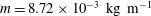 $m=8.72\times 10^{-3}~\text{kg}~\text{m}^{-1}$
, displaced mass per unit length
$m=8.72\times 10^{-3}~\text{kg}~\text{m}^{-1}$
, displaced mass per unit length
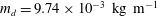 $m_{d}=9.74\times 10^{-3}~\text{kg}~\text{m}^{-1}$
and added mass per unit length
$m_{d}=9.74\times 10^{-3}~\text{kg}~\text{m}^{-1}$
and added mass per unit length
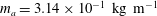 $m_{a}=3.14\times 10^{-1}~\text{kg}~\text{m}^{-1}$
. Thus,
$m_{a}=3.14\times 10^{-1}~\text{kg}~\text{m}^{-1}$
. Thus,
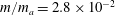 $m/m_{a}=2.8\times 10^{-2}$
and
$m/m_{a}=2.8\times 10^{-2}$
and
 $m_{d}/m_{a}=3.1\times 10^{-2}$
so that the structural inertia and the virtual buoyancy are indeed negligible. In order to get the desired relative flow, we forced the clamped edge of the blade into an oscillatory translation of opposite velocity
$m_{d}/m_{a}=3.1\times 10^{-2}$
so that the structural inertia and the virtual buoyancy are indeed negligible. In order to get the desired relative flow, we forced the clamped edge of the blade into an oscillatory translation of opposite velocity
 $-\boldsymbol{U}(t)$
and analysed the dynamic deformation of the structure in the oscillating frame. The flexible structure is clamped at the bottom of a vertical rigid rod and fully immersed in a rectangular water tank of horizontal dimensions 58
$-\boldsymbol{U}(t)$
and analysed the dynamic deformation of the structure in the oscillating frame. The flexible structure is clamped at the bottom of a vertical rigid rod and fully immersed in a rectangular water tank of horizontal dimensions 58
 $\times$
35 cm and 48 cm of water depth. The rod crossing the free surface is streamlined in the direction of the motion in order to induce as little perturbation as possible in the fluid. The forcing motion is obtained through a DC motor driving an arm of length
$\times$
35 cm and 48 cm of water depth. The rod crossing the free surface is streamlined in the direction of the motion in order to induce as little perturbation as possible in the fluid. The forcing motion is obtained through a DC motor driving an arm of length
 $A$
in rotation. The speed of rotation
$A$
in rotation. The speed of rotation
 $\unicode[STIX]{x1D6FA}$
is tuned by changing the voltage at the terminals of the motor. The arm is attached to a carriage freely translating on a vertical rail, which in turn is fixed on an another carriage sliding on an horizontal rail. The mounting rod is linked to the latter carriage so that it is driven into the desired sinusoidal translation of amplitude
$\unicode[STIX]{x1D6FA}$
is tuned by changing the voltage at the terminals of the motor. The arm is attached to a carriage freely translating on a vertical rail, which in turn is fixed on an another carriage sliding on an horizontal rail. The mounting rod is linked to the latter carriage so that it is driven into the desired sinusoidal translation of amplitude
 $A$
and angular frequency
$A$
and angular frequency
 $\unicode[STIX]{x1D6FA}$
as the arm rotates. The amplitude
$\unicode[STIX]{x1D6FA}$
as the arm rotates. The amplitude
 $A$
could be varied continuously between 5.4 (
$A$
could be varied continuously between 5.4 (
 $\unicode[STIX]{x1D6FC}=0.27$
) and 13 cm (
$\unicode[STIX]{x1D6FC}=0.27$
) and 13 cm (
 $\unicode[STIX]{x1D6FC}=0.65$
), and the frequency between 0.21 (
$\unicode[STIX]{x1D6FC}=0.65$
), and the frequency between 0.21 (
 $\unicode[STIX]{x1D714}=2.3$
) and 1.08 Hz (
$\unicode[STIX]{x1D714}=2.3$
) and 1.08 Hz (
 $\unicode[STIX]{x1D714}=12.0$
). The motion of the whole structure is filmed with a fixed camera in front of the tank at 100 fps and the position and deformation of the blade through time is extracted from each frame. The deformation in the oscillating frame is then phase averaged over a minimum of 10 cycles to get a unique cycle representative of the whole run.
$\unicode[STIX]{x1D714}=12.0$
). The motion of the whole structure is filmed with a fixed camera in front of the tank at 100 fps and the position and deformation of the blade through time is extracted from each frame. The deformation in the oscillating frame is then phase averaged over a minimum of 10 cycles to get a unique cycle representative of the whole run.
The results for three different amplitudes and frequencies spanning the experimental domain are shown in figure 3. In this range of forcing parameters, we notice a diversity of behaviours. For a given frequency ratio
 $\unicode[STIX]{x1D714}$
, the maximum deflection of the blade increases with the amplitude of the forcing
$\unicode[STIX]{x1D714}$
, the maximum deflection of the blade increases with the amplitude of the forcing
 $\unicode[STIX]{x1D6FC}$
. However, the horizontal excursion of the structure is obviously limited by its own length, so the amplitude of the motion has to saturate when
$\unicode[STIX]{x1D6FC}$
. However, the horizontal excursion of the structure is obviously limited by its own length, so the amplitude of the motion has to saturate when
 $\unicode[STIX]{x1D6FC}$
is increased even more. Besides, the maximum deflection is clearly increasing with the forcing frequency for the largest forcing amplitude
$\unicode[STIX]{x1D6FC}$
is increased even more. Besides, the maximum deflection is clearly increasing with the forcing frequency for the largest forcing amplitude
 $\unicode[STIX]{x1D6FC}=0.65$
, but this is much less obvious for the smallest amplitude
$\unicode[STIX]{x1D6FC}=0.65$
, but this is much less obvious for the smallest amplitude
 $\unicode[STIX]{x1D6FC}=0.27$
. On the other hand, for any given forcing amplitude
$\unicode[STIX]{x1D6FC}=0.27$
. On the other hand, for any given forcing amplitude
 $\unicode[STIX]{x1D6FC}$
, the dynamics of the deformation is greatly affected when the forcing frequency is increased. For the smallest frequency ratio
$\unicode[STIX]{x1D6FC}$
, the dynamics of the deformation is greatly affected when the forcing frequency is increased. For the smallest frequency ratio
 $\unicode[STIX]{x1D714}=2.3$
, the tip follows the same trajectory during both half-cycles and remains close to the unit circle. The motion of the whole blade is therefore approximately in phase, and curvature is concentrated near the clamped edge while the rest of the beam remains straight. This deforming shape is similar to the static reconfiguration that occurs in steady flow (Gosselin et al.
Reference Gosselin, de Langre and Machado-Almeida2010). Conversely, when the frequency is increased, the tip follows a figure-of-eight trajectory and we notice curvature waves propagating along the span in the course of the cycle indicating an increasing spanwise phase shift. This indicates a highly dynamic response that cannot be considered quasi-steady a priori. Besides, the propagation of curvature waves may induce large loads anywhere along the span and not restricted to the clamping point.
$\unicode[STIX]{x1D714}=2.3$
, the tip follows the same trajectory during both half-cycles and remains close to the unit circle. The motion of the whole blade is therefore approximately in phase, and curvature is concentrated near the clamped edge while the rest of the beam remains straight. This deforming shape is similar to the static reconfiguration that occurs in steady flow (Gosselin et al.
Reference Gosselin, de Langre and Machado-Almeida2010). Conversely, when the frequency is increased, the tip follows a figure-of-eight trajectory and we notice curvature waves propagating along the span in the course of the cycle indicating an increasing spanwise phase shift. This indicates a highly dynamic response that cannot be considered quasi-steady a priori. Besides, the propagation of curvature waves may induce large loads anywhere along the span and not restricted to the clamping point.

Figure 3. Phase-averaged experimental oscillation cycle for varying amplitudes
 $\unicode[STIX]{x1D6FC}$
and frequencies
$\unicode[STIX]{x1D6FC}$
and frequencies
 $\unicode[STIX]{x1D714}$
. Snapshots of the structural shape (——) and tip trajectory (– –).
$\unicode[STIX]{x1D714}$
. Snapshots of the structural shape (——) and tip trajectory (– –).
In order to validate the numerical model of § 2, we also compared these experimental observations to the output of the numerical simulations. As shown in figure 4(a), the numerical results for the amplitude of deflection at the tip
 $X_{tip}$
match very closely the experimental measurements. The snapshots displayed in figure 4(b) for two cases at the boundaries of our experimental domain (indicated in figure 4
a) also show very good agreement between the observations and the simulations. Additional experimental validation of the model for smaller forcing amplitudes can be found in Piñeirua et al. (Reference Piñeirua, Thiria and Godoy-Diana2017).
$X_{tip}$
match very closely the experimental measurements. The snapshots displayed in figure 4(b) for two cases at the boundaries of our experimental domain (indicated in figure 4
a) also show very good agreement between the observations and the simulations. Additional experimental validation of the model for smaller forcing amplitudes can be found in Piñeirua et al. (Reference Piñeirua, Thiria and Godoy-Diana2017).

Figure 4. Comparison between experimental observations and numerical simulations. (a) Amplitude of the deflection at the tip against the frequency ratio, for
 $\unicode[STIX]{x1D6FC}=0.27$
(numerical – –, experimental ○),
$\unicode[STIX]{x1D6FC}=0.27$
(numerical – –, experimental ○),
 $\unicode[STIX]{x1D6FC}=0.65$
(numerical ——, experimental ▵). (b) Deformed shape found experimentally (left) and numerically (right), in case A (top,
$\unicode[STIX]{x1D6FC}=0.65$
(numerical ——, experimental ▵). (b) Deformed shape found experimentally (left) and numerically (right), in case A (top,
 $\unicode[STIX]{x1D6FC}=0.27$
,
$\unicode[STIX]{x1D6FC}=0.27$
,
 $\unicode[STIX]{x1D714}=2.3$
) and case B (bottom,
$\unicode[STIX]{x1D714}=2.3$
) and case B (bottom,
 $\unicode[STIX]{x1D6FC}=0.65$
,
$\unicode[STIX]{x1D6FC}=0.65$
,
 $\unicode[STIX]{x1D714}=12.0$
).
$\unicode[STIX]{x1D714}=12.0$
).
These results confirm the validity of our model, and we will therefore use it in the following to systematically explore the parameter space within and beyond the experimentally accessible range.
4 Kinematics
4.1 Small amplitude of flow oscillation
 $\unicode[STIX]{x1D6FC}=A/L\ll 1$

Let us first consider the situation where the amplitude of forcing is small (
 $\unicode[STIX]{x1D6FC}\ll 1$
). The excursion of the fluid particles being small compared to the length of the blade, we may also assume that the deflection remains small as well
$\unicode[STIX]{x1D6FC}\ll 1$
). The excursion of the fluid particles being small compared to the length of the blade, we may also assume that the deflection remains small as well
 $|x(s,t)|\ll 1$
. Neglecting all the geometrical nonlinearities in (2.8) thus yields the small-amplitude equation
$|x(s,t)|\ll 1$
. Neglecting all the geometrical nonlinearities in (2.8) thus yields the small-amplitude equation
 $$\begin{eqnarray}x^{(4)}+\ddot{x}=\unicode[STIX]{x1D6FC}\unicode[STIX]{x1D714}^{2}\cos (\unicode[STIX]{x1D714}t)-\unicode[STIX]{x1D706}|{\dot{x}}-\unicode[STIX]{x1D6FC}\unicode[STIX]{x1D714}\sin (\unicode[STIX]{x1D714}t)|({\dot{x}}-\unicode[STIX]{x1D6FC}\unicode[STIX]{x1D714}\sin (\unicode[STIX]{x1D714}t)),\end{eqnarray}$$
with boundary conditions
 $x=x^{\prime }=0$
at
$x=x^{\prime }=0$
at
 $s=0$
and
$s=0$
and
 $x^{\prime \prime }=x^{\prime \prime \prime }=0$
at
$x^{\prime \prime }=x^{\prime \prime \prime }=0$
at
 $s=1$
. Equation (4.1) is the standard cantilever beam linear oscillator, forced on the right-hand side by the fluid inertia and the resistive drag. Note that only the nonlinearities of geometrical nature have been removed but the quadratic relative velocity term of the resistive drag has been retained at this point. Indeed, the slenderness parameter
$s=1$
. Equation (4.1) is the standard cantilever beam linear oscillator, forced on the right-hand side by the fluid inertia and the resistive drag. Note that only the nonlinearities of geometrical nature have been removed but the quadratic relative velocity term of the resistive drag has been retained at this point. Indeed, the slenderness parameter
 $\unicode[STIX]{x1D706}$
that scales this term is large and the order of magnitude of the whole resistive drag term depends as much on the scaling of
$\unicode[STIX]{x1D706}$
that scales this term is large and the order of magnitude of the whole resistive drag term depends as much on the scaling of
 $\unicode[STIX]{x1D706}$
as it depends on that of
$\unicode[STIX]{x1D706}$
as it depends on that of
 $\unicode[STIX]{x1D6FC}$
. Besides, no assumption has been made regarding the characteristic time scale for the variations of
$\unicode[STIX]{x1D6FC}$
. Besides, no assumption has been made regarding the characteristic time scale for the variations of
 $x$
, and there is no reason to presume that
$x$
, and there is no reason to presume that
 ${\dot{x}}$
should be small compared to the free-stream velocity based on the sole assumption that
${\dot{x}}$
should be small compared to the free-stream velocity based on the sole assumption that
 $x$
is small.
$x$
is small.
If the period of the forcing is large compared to the characteristic response time of the structure (
 $\unicode[STIX]{x1D714}<1$
), we may assume that the structure is in static equilibrium with the fluid forcing at all times. Consequently, we may neglect the velocity and acceleration of the structure and (4.1) reduces to the small-amplitude static equation
$\unicode[STIX]{x1D714}<1$
), we may assume that the structure is in static equilibrium with the fluid forcing at all times. Consequently, we may neglect the velocity and acceleration of the structure and (4.1) reduces to the small-amplitude static equation
 $$\begin{eqnarray}x^{(4)}=\unicode[STIX]{x1D6FC}\unicode[STIX]{x1D714}^{2}[\cos (\unicode[STIX]{x1D714}t)+(\unicode[STIX]{x1D706}\unicode[STIX]{x1D6FC})|\text{sin}(\unicode[STIX]{x1D714}t)|\sin (\unicode[STIX]{x1D714}t)].\end{eqnarray}$$
The left-hand side of this equation now involves only the linearized stiffness force, while the fluid forcing on the right-hand side is the same as that a perfectly rigid blade would endure.
On the other hand, if the forcing varies with a period comparable to the characteristic structural response time or faster (
 $\unicode[STIX]{x1D714}>1$
), we may then assume that the amplitude and the frequency of the response will scale as those of the forcing, as is usually the case for linear oscillators (see for instance Blevins Reference Blevins1990). We thus define the rescaled deflection and time
$\unicode[STIX]{x1D714}>1$
), we may then assume that the amplitude and the frequency of the response will scale as those of the forcing, as is usually the case for linear oscillators (see for instance Blevins Reference Blevins1990). We thus define the rescaled deflection and time
 $\tilde{x}=x/\unicode[STIX]{x1D6FC}$
,
$\tilde{x}=x/\unicode[STIX]{x1D6FC}$
,
 $\tilde{t}=\unicode[STIX]{x1D714}t$
, so that the small-amplitude equation (4.1) can be written
$\tilde{t}=\unicode[STIX]{x1D714}t$
, so that the small-amplitude equation (4.1) can be written
 $$\begin{eqnarray}\frac{1}{\unicode[STIX]{x1D714}^{2}}\tilde{x}^{(4)}+\ddot{\tilde{x}}=\cos (\tilde{t})-K_{C}|\dot{\tilde{x}}-\sin (\tilde{t})|(\dot{\tilde{x}}-\sin (\tilde{t})),\end{eqnarray}$$
which now only depends on two parameters: the frequency parameter
 $\unicode[STIX]{x1D714}$
and a new amplitude parameter
$\unicode[STIX]{x1D714}$
and a new amplitude parameter
 $K_{C}=\unicode[STIX]{x1D706}\unicode[STIX]{x1D6FC}=(2C_{D}/\unicode[STIX]{x03C0})A/W$
that compares the fluid particles excursion to the width instead of the length of the blade. This parameter is a problem-specific formulation of the classical Keulegan–Carpenter number that compares the respective magnitudes of the drag and the fluid inertial forces. When
$K_{C}=\unicode[STIX]{x1D706}\unicode[STIX]{x1D6FC}=(2C_{D}/\unicode[STIX]{x03C0})A/W$
that compares the fluid particles excursion to the width instead of the length of the blade. This parameter is a problem-specific formulation of the classical Keulegan–Carpenter number that compares the respective magnitudes of the drag and the fluid inertial forces. When
 $K_{C}$
is small, the fluid inertia dominates over drag and vice versa.
$K_{C}$
is small, the fluid inertia dominates over drag and vice versa.
Let us first look at the asymptotic limit of infinitely small amplitude of the forcing
 $K_{C}\rightarrow 0$
. The nonlinear drag term can be neglected and (4.3) then simply describes a linear oscillator with sinusoidal forcing due to the fluid inertial term. It can be solved analytically and the solution is
$K_{C}\rightarrow 0$
. The nonlinear drag term can be neglected and (4.3) then simply describes a linear oscillator with sinusoidal forcing due to the fluid inertial term. It can be solved analytically and the solution is
 $$\begin{eqnarray}\tilde{x}(s,\tilde{t})=2\mathop{\sum }_{m=0}^{+\infty }\frac{\unicode[STIX]{x1D70E}_{m}}{k_{m}}\frac{\unicode[STIX]{x1D714}^{2}}{k_{m}^{4}-\unicode[STIX]{x1D714}^{2}}X_{m}(s)\cos \tilde{t},\end{eqnarray}$$
with the wavenumbers
 $k_{m}$
satisfying
$k_{m}$
satisfying
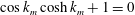 $\cos k_{m}\cosh k_{m}+1=0$
, the classical cantilever beam modes
$\cos k_{m}\cosh k_{m}+1=0$
, the classical cantilever beam modes
 $X_{m}(s)=[\cosh (k_{m}s)-\cos (k_{m}s)]-\unicode[STIX]{x1D70E}_{m}[\sinh (k_{m}s)-\sin (k_{m}s)]$
and
$X_{m}(s)=[\cosh (k_{m}s)-\cos (k_{m}s)]-\unicode[STIX]{x1D70E}_{m}[\sinh (k_{m}s)-\sin (k_{m}s)]$
and
 $\unicode[STIX]{x1D70E}_{m}=(\sinh k_{m}-\sin k_{m})/(\cosh k_{m}+\cos k_{m})$
(see Weaver, Timoshenko & Young Reference Weaver, Timoshenko and Young1990).
$\unicode[STIX]{x1D70E}_{m}=(\sinh k_{m}-\sin k_{m})/(\cosh k_{m}+\cos k_{m})$
(see Weaver, Timoshenko & Young Reference Weaver, Timoshenko and Young1990).
Figure 5(a) compares the amplitude of the maximum deflection for different values of
 $K_{C}$
, and for the asymptotic solution (4.4), as a function of
$K_{C}$
, and for the asymptotic solution (4.4), as a function of
 $\unicode[STIX]{x1D714}$
. This analytical solution is in good agreement with the model predictions for any
$\unicode[STIX]{x1D714}$
. This analytical solution is in good agreement with the model predictions for any
 $K_{C}\leqslant 1$
, and it shows that the system behaves as a high-pass filter in this range of the parameter space. As the frequency increases, successive beam modes are excited and resonances occur when the frequency of the forcing matches one of the natural modes of the structure
$K_{C}\leqslant 1$
, and it shows that the system behaves as a high-pass filter in this range of the parameter space. As the frequency increases, successive beam modes are excited and resonances occur when the frequency of the forcing matches one of the natural modes of the structure
 $\unicode[STIX]{x1D714}=k_{m}^{2}$
. For finite but small
$\unicode[STIX]{x1D714}=k_{m}^{2}$
. For finite but small
 $K_{C}$
, drag acts as a damping term that saturates the amplitude of the resonances but does not seem to affect significantly the modal shape of the deforming structure. The deformation of the beam close to the first three resonances (
$K_{C}$
, drag acts as a damping term that saturates the amplitude of the resonances but does not seem to affect significantly the modal shape of the deforming structure. The deformation of the beam close to the first three resonances (
 $\unicode[STIX]{x1D714}_{1}=3.5$
,
$\unicode[STIX]{x1D714}_{1}=3.5$
,
 $\unicode[STIX]{x1D714}_{2}=22.0$
,
$\unicode[STIX]{x1D714}_{2}=22.0$
,
 $\unicode[STIX]{x1D714}_{3}=61.7$
) for
$\unicode[STIX]{x1D714}_{3}=61.7$
) for
 $K_{C}=10^{-2}$
in figure 5(b) is indeed similar to the corresponding beam modes
$K_{C}=10^{-2}$
in figure 5(b) is indeed similar to the corresponding beam modes
 $X_{1}$
,
$X_{1}$
,
 $X_{2}$
,
$X_{2}$
,
 $X_{3}$
involved in the asymptotic solution (4.4). Note that when
$X_{3}$
involved in the asymptotic solution (4.4). Note that when
 $K_{C}$
is close to 1, the nonlinear drag term is also responsible for a drift of the resonance frequencies that has been studied in Arellano Castro et al. (Reference Arellano Castro, Guillamot, Cros and Eloy2014). This effect is not obvious in figure 5(a) because of the very strong attenuation of the resonance peak for
$K_{C}$
is close to 1, the nonlinear drag term is also responsible for a drift of the resonance frequencies that has been studied in Arellano Castro et al. (Reference Arellano Castro, Guillamot, Cros and Eloy2014). This effect is not obvious in figure 5(a) because of the very strong attenuation of the resonance peak for
 $K_{C}=1$
, but is more visible in the structural stress analysis of figure 9(a).
$K_{C}=1$
, but is more visible in the structural stress analysis of figure 9(a).

Figure 5. (a) Amplitude of the maximum scaled deflection obtained with (4.3) against the frequency ratio.
 $K_{C}=10^{-2}$
(——),
$K_{C}=10^{-2}$
(——),
 $K_{C}=10^{0}$
(– – –),
$K_{C}=10^{0}$
(– – –),
 $K_{C}=10^{2}$
(— ⋅ —). Analytical solution for
$K_{C}=10^{2}$
(— ⋅ —). Analytical solution for
 $K_{C}\rightarrow 0$
(
$K_{C}\rightarrow 0$
(
 $\cdots \cdots$
). (b) Snapshots of the beam over one cycle obtained with (4.3) for
$\cdots \cdots$
). (b) Snapshots of the beam over one cycle obtained with (4.3) for
 $K_{C}=10^{-2}$
(modal regime) and for
$K_{C}=10^{-2}$
(modal regime) and for
 $\unicode[STIX]{x1D714}=\unicode[STIX]{x1D714}_{1}$
(resonance of mode 1),
$\unicode[STIX]{x1D714}=\unicode[STIX]{x1D714}_{1}$
(resonance of mode 1),
 $\unicode[STIX]{x1D714}=\unicode[STIX]{x1D714}_{2}$
(resonance of mode 2),
$\unicode[STIX]{x1D714}=\unicode[STIX]{x1D714}_{2}$
(resonance of mode 2),
 $\unicode[STIX]{x1D714}=\unicode[STIX]{x1D714}_{3}$
(resonance of mode 3). (c) Same as (b) but with
$\unicode[STIX]{x1D714}=\unicode[STIX]{x1D714}_{3}$
(resonance of mode 3). (c) Same as (b) but with
 $K_{C}=10^{2}$
(convective regime).
$K_{C}=10^{2}$
(convective regime).
On the other hand, if we increase the fluid particles excursion beyond the width of the structure (
 $K_{C}\gg 1$
), a change in physical behaviour occurs. Drag becomes the dominant term in (4.3). The leading-order solution now is
$K_{C}\gg 1$
), a change in physical behaviour occurs. Drag becomes the dominant term in (4.3). The leading-order solution now is
 $\tilde{x}(s,\tilde{t})=\cos \tilde{t}$
, which amounts to considering that the structure is convected exactly with the fluid particles. Therefore, we may call this regime the convective regime. This solution is however incompatible with the boundary condition at the clamped edge
$\tilde{x}(s,\tilde{t})=\cos \tilde{t}$
, which amounts to considering that the structure is convected exactly with the fluid particles. Therefore, we may call this regime the convective regime. This solution is however incompatible with the boundary condition at the clamped edge
 $\tilde{x}(0,\tilde{t})=0$
, so an elastic boundary layer develops close to the clamping point. The relative magnitude of the terms in (4.3) suggests that the thickness of the boundary layer scales as
$\tilde{x}(0,\tilde{t})=0$
, so an elastic boundary layer develops close to the clamping point. The relative magnitude of the terms in (4.3) suggests that the thickness of the boundary layer scales as
 $\unicode[STIX]{x1D6FF}=(K_{C}\,\unicode[STIX]{x1D714}^{2})^{-1/4}$
. Rescaling the curvilinear coordinate
$\unicode[STIX]{x1D6FF}=(K_{C}\,\unicode[STIX]{x1D714}^{2})^{-1/4}$
. Rescaling the curvilinear coordinate
 ${\hat{s}}=s/\unicode[STIX]{x1D6FF}$
in (4.3) provides the leading-order equation for the inner solution
${\hat{s}}=s/\unicode[STIX]{x1D6FF}$
in (4.3) provides the leading-order equation for the inner solution
 $$\begin{eqnarray}\unicode[STIX]{x2202}_{{\hat{s}}}^{4}\tilde{x}=|\dot{\tilde{x}}-\sin (\tilde{t})|(\dot{\tilde{x}}-\sin (\tilde{t})),\end{eqnarray}$$
with boundary conditions
 $\tilde{x}=\unicode[STIX]{x2202}_{{\hat{s}}}\tilde{x}=0$
at
$\tilde{x}=\unicode[STIX]{x2202}_{{\hat{s}}}\tilde{x}=0$
at
 ${\hat{s}}=0$
and
${\hat{s}}=0$
and
 $\unicode[STIX]{x2202}_{{\hat{s}}}^{2}\tilde{x}=\unicode[STIX]{x2202}_{{\hat{s}}}^{3}\tilde{x}=0$
at
$\unicode[STIX]{x2202}_{{\hat{s}}}^{2}\tilde{x}=\unicode[STIX]{x2202}_{{\hat{s}}}^{3}\tilde{x}=0$
at
 ${\hat{s}}=1/\unicode[STIX]{x1D6FF}$
.
${\hat{s}}=1/\unicode[STIX]{x1D6FF}$
.
The dynamic deformation of the structure displayed in figure 5(c) for
 $K_{C}=10^{2}$
for the same values of frequency ratios as in figure 5(b) clearly shows the concentration of the curvature close to the clamped edge and the passive convection of the main part of the structure. The resonances previously observed in the modal regime in figure 5(a) are now completely damped out when
$K_{C}=10^{2}$
for the same values of frequency ratios as in figure 5(b) clearly shows the concentration of the curvature close to the clamped edge and the passive convection of the main part of the structure. The resonances previously observed in the modal regime in figure 5(a) are now completely damped out when
 $K_{C}=10^{2}$
. Compared to the case
$K_{C}=10^{2}$
. Compared to the case
 $K_{C}=1$
, this curve is shifted one decade to the left as the proper scaling parameter is now
$K_{C}=1$
, this curve is shifted one decade to the left as the proper scaling parameter is now
 $\sqrt{K_{C}}\,\unicode[STIX]{x1D714}$
instead of
$\sqrt{K_{C}}\,\unicode[STIX]{x1D714}$
instead of
 $\unicode[STIX]{x1D714}$
, and
$\unicode[STIX]{x1D714}$
, and
 $\sqrt{K_{C}}=10$
for
$\sqrt{K_{C}}=10$
for
 $K_{C}=10^{2}$
. The scaling of the boundary layer thickness
$K_{C}=10^{2}$
. The scaling of the boundary layer thickness
 $\unicode[STIX]{x1D6FF}$
is similar to that of the effective length of Luhar & Nepf (Reference Luhar and Nepf2016), as it is based on the equilibrium between the same forces. A similar problem had also been considered in Mullarney & Henderson (Reference Mullarney and Henderson2010). In the case of a wave-like flow, the authors neglected the quadratic nonlinearity in order to get an analytical solution.
$\unicode[STIX]{x1D6FF}$
is similar to that of the effective length of Luhar & Nepf (Reference Luhar and Nepf2016), as it is based on the equilibrium between the same forces. A similar problem had also been considered in Mullarney & Henderson (Reference Mullarney and Henderson2010). In the case of a wave-like flow, the authors neglected the quadratic nonlinearity in order to get an analytical solution.
4.2 Large amplitude of flow oscillation
$\unicode[STIX]{x1D6FC}=A/L\gg 1$

In the convective regime discussed above, the structure is purely convected with the fluid particles on most of its span over the whole cycle. But when the amplitude becomes larger than the length of the structure, geometric saturation of the deflection occurs because the structure cannot extend further than its own length. The deflection is now of order
 $x=O(1)$
and so we cannot neglect the geometrical nonlinearities of (2.8) anymore. The slenderness
$x=O(1)$
and so we cannot neglect the geometrical nonlinearities of (2.8) anymore. The slenderness
 $\unicode[STIX]{x1D706}$
becomes the relevant parameter to compare drag to the fluid inertial forces in lieu of the Keulegan–Carpenter number
$\unicode[STIX]{x1D706}$
becomes the relevant parameter to compare drag to the fluid inertial forces in lieu of the Keulegan–Carpenter number
 $K_{C}$
. Because we only consider elongated structures
$K_{C}$
. Because we only consider elongated structures
 $\unicode[STIX]{x1D706}\gg 1$
in this study, drag will always be the dominant term in the large-amplitude regime.
$\unicode[STIX]{x1D706}\gg 1$
in this study, drag will always be the dominant term in the large-amplitude regime.
The dynamic deformations obtained with (2.8) in two cases with similar amplitude
 $\unicode[STIX]{x1D6FC}=10^{2}$
and slenderness
$\unicode[STIX]{x1D6FC}=10^{2}$
and slenderness
 $\unicode[STIX]{x1D706}=12.7$
but different frequencies are compared in figure 6 with 100 snapshots per cycle with constant time interval. In the small frequency case (a), the deformation looks quasi-static. Transition from one side to the other is slow (many snapshots distributed from left to right) and the curvature is essentially concentrated near the clamped edge during the whole cycle. On the other hand, in the larger frequency case (b), the structure switches sides very fast (few snapshots visible in the centre while many are superimposed on the sides) and curvature waves propagate very quickly along the span during reversal. Therefore, the cycle may be decomposed into two steps: first, a fast reversal period during which the structure switches from one side to the other immediately after flow reversal, followed by a longer period of quasi-static adaptation to the increasing magnitude of the drag. Because the dominant drag force
$\unicode[STIX]{x1D706}=12.7$
but different frequencies are compared in figure 6 with 100 snapshots per cycle with constant time interval. In the small frequency case (a), the deformation looks quasi-static. Transition from one side to the other is slow (many snapshots distributed from left to right) and the curvature is essentially concentrated near the clamped edge during the whole cycle. On the other hand, in the larger frequency case (b), the structure switches sides very fast (few snapshots visible in the centre while many are superimposed on the sides) and curvature waves propagate very quickly along the span during reversal. Therefore, the cycle may be decomposed into two steps: first, a fast reversal period during which the structure switches from one side to the other immediately after flow reversal, followed by a longer period of quasi-static adaptation to the increasing magnitude of the drag. Because the dominant drag force
 $\unicode[STIX]{x1D706}|U_{n}|U_{n}\propto \unicode[STIX]{x1D706}\unicode[STIX]{x1D6FC}^{2}\unicode[STIX]{x1D714}^{2}$
is proportional to
$\unicode[STIX]{x1D706}|U_{n}|U_{n}\propto \unicode[STIX]{x1D706}\unicode[STIX]{x1D6FC}^{2}\unicode[STIX]{x1D714}^{2}$
is proportional to
 $\unicode[STIX]{x1D714}^{2}$
, the maximum drag is larger in the large frequency case in figure 6, which explains why the maximum deflection is enhanced.
$\unicode[STIX]{x1D714}^{2}$
, the maximum drag is larger in the large frequency case in figure 6, which explains why the maximum deflection is enhanced.

Figure 6. Snapshots of the deforming structure over one cycle (——) and tip trajectory (– – –) obtained with (2.8) for
 $\unicode[STIX]{x1D706}=12.7$
,
$\unicode[STIX]{x1D706}=12.7$
,
 $\unicode[STIX]{x1D6FC}=10^{2}$
. (a)
$\unicode[STIX]{x1D6FC}=10^{2}$
. (a)
 $\unicode[STIX]{x1D714}=10^{-2}$
, (b)
$\unicode[STIX]{x1D714}=10^{-2}$
, (b)
 $\unicode[STIX]{x1D714}=1$
.
$\unicode[STIX]{x1D714}=1$
.
To estimate the time scale of reversal
 $T_{r}$
, let us assume that shortly before flow reversal, the structure is fully reconfigured on one side
$T_{r}$
, let us assume that shortly before flow reversal, the structure is fully reconfigured on one side
 $x(s=1,t=0)=-1$
. At flow reversal
$x(s=1,t=0)=-1$
. At flow reversal
 $t=0$
, drag starts pushing the structure to the other side. Let us assume that the blade is purely convected until it is fully reconfigured on the other side at the end of the reversal time
$t=0$
, drag starts pushing the structure to the other side. Let us assume that the blade is purely convected until it is fully reconfigured on the other side at the end of the reversal time
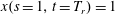 $x(s=1,t=T_{r})=1$
. In that case, we may write
$x(s=1,t=T_{r})=1$
. In that case, we may write
 $$\begin{eqnarray}2=x_{tip}(T_{r})-x_{tip}(0)=\int _{0}^{T_{r}}\unicode[STIX]{x1D6FC}\unicode[STIX]{x1D714}\sin (\unicode[STIX]{x1D714}t)\,\text{d}t\simeq \int _{0}^{T_{r}}\unicode[STIX]{x1D6FC}\unicode[STIX]{x1D714}^{2}t\,\text{d}t=\frac{1}{2}\unicode[STIX]{x1D6FC}(\unicode[STIX]{x1D714}T_{r})^{2},\end{eqnarray}$$
where the linearization holds owing to the fact that reversal occurs on a time scale much smaller than the period of the cycle (
 $\unicode[STIX]{x1D714}T_{r}\ll 2\unicode[STIX]{x03C0}$
). We finally obtain
$\unicode[STIX]{x1D714}T_{r}\ll 2\unicode[STIX]{x03C0}$
). We finally obtain
 $T_{r}=2/(\unicode[STIX]{x1D714}\sqrt{\unicode[STIX]{x1D6FC}})$
. This expression of the reversal time is normalized by the scale of the natural period of the structure. It is more relevant than
$T_{r}=2/(\unicode[STIX]{x1D714}\sqrt{\unicode[STIX]{x1D6FC}})$
. This expression of the reversal time is normalized by the scale of the natural period of the structure. It is more relevant than
 $\unicode[STIX]{x1D714}$
to assess the quasi-steady nature of the deformation in the large-amplitude regime because it compares only the time scale on which structural motion is significant (instead of the whole cycle period) to the characteristic structural response time. Indeed, in figure 6(a), the large reversal time
$\unicode[STIX]{x1D714}$
to assess the quasi-steady nature of the deformation in the large-amplitude regime because it compares only the time scale on which structural motion is significant (instead of the whole cycle period) to the characteristic structural response time. Indeed, in figure 6(a), the large reversal time
 $T_{r}=20$
allows the structure to be in quasi-static equilibrium with the fluid loading at all times. Conversely, in figure 6(b) the small reversal time
$T_{r}=20$
allows the structure to be in quasi-static equilibrium with the fluid loading at all times. Conversely, in figure 6(b) the small reversal time
 $T_{r}=0.2$
is responsible for the propagation of curvature waves during reversal. Hence, when
$T_{r}=0.2$
is responsible for the propagation of curvature waves during reversal. Hence, when
 $T_{r}\gg 1$
, the structure is in static equilibrium with the fluid forces during the whole cycle, while the quasi-static character of the deformation is lost during the fast reversal when
$T_{r}\gg 1$
, the structure is in static equilibrium with the fluid forces during the whole cycle, while the quasi-static character of the deformation is lost during the fast reversal when
 $T_{r}\ll 1$
.
$T_{r}\ll 1$
.
A zoom on the trajectory of the tip around flow reversal in the case of figure 6(b) shown in figure 7 (solid line) confirms that reversal occurs approximately between
 $t/T_{r}=0$
and
$t/T_{r}=0$
and
 $t/T_{r}=1$
. When the slenderness parameter is increased (broken lines,
$t/T_{r}=1$
. When the slenderness parameter is increased (broken lines,
 $\unicode[STIX]{x1D706}=127$
), the time scale of the dynamics remains unchanged. The same graphs for the same
$\unicode[STIX]{x1D706}=127$
), the time scale of the dynamics remains unchanged. The same graphs for the same
 $T_{r}$
but for a smaller or a larger amplitude (
$T_{r}$
but for a smaller or a larger amplitude (
 $\unicode[STIX]{x1D6FC}=10$
and
$\unicode[STIX]{x1D6FC}=10$
and
 $\unicode[STIX]{x1D6FC}=10^{3}$
respectively), not shown here, are practically indistinguishable from that in figure 7. This result confirms that the amplitude and frequency parameters influence the kinematics of the reversal exclusively through the combined parameter
$\unicode[STIX]{x1D6FC}=10^{3}$
respectively), not shown here, are practically indistinguishable from that in figure 7. This result confirms that the amplitude and frequency parameters influence the kinematics of the reversal exclusively through the combined parameter
 $T_{r}$
. Besides, because the structural mass was neglected, no dynamic excitation possibly resulting from the violent reversal is allowed to persist after
$T_{r}$
. Besides, because the structural mass was neglected, no dynamic excitation possibly resulting from the violent reversal is allowed to persist after
 $T_{r}$
.
$T_{r}$
.

Figure 7. Horizontal displacement of the tip during flow reversal against the rescaled time
 $t/T_{r}$
, for
$t/T_{r}$
, for
 $\unicode[STIX]{x1D6FC}=10^{2}$
,
$\unicode[STIX]{x1D6FC}=10^{2}$
,
 $T_{r}=0.2$
(
$T_{r}=0.2$
(
 $\unicode[STIX]{x1D714}=1$
) and
$\unicode[STIX]{x1D714}=1$
) and
 $\unicode[STIX]{x1D706}=12.7$
(——),
$\unicode[STIX]{x1D706}=12.7$
(——),
 $\unicode[STIX]{x1D706}=127$
(– – –).
$\unicode[STIX]{x1D706}=127$
(– – –).

Figure 8. Schematic view of the kinematic regimes in the amplitude–frequency space.
4.3 Summary of the kinematic regimes
So far we have found that depending on the amplitude and frequency of the oscillating flow with respect to the dimensions and natural frequencies of the blade, four different kinematic regimes may exist. Their respective locations in the parameter space are summarized in figure 8.
First, if the amplitude is much smaller than the length of the blade (
 $\unicode[STIX]{x1D6FC}\ll 1$
or equivalently
$\unicode[STIX]{x1D6FC}\ll 1$
or equivalently
 $A\ll L$
) and the frequency of the flow smaller than that of the structure (
$A\ll L$
) and the frequency of the flow smaller than that of the structure (
 $\unicode[STIX]{x1D714}<1$
or equivalently
$\unicode[STIX]{x1D714}<1$
or equivalently
 $\unicode[STIX]{x1D6FA}<1/T_{s}$
), the structure is in static equilibrium with the fluid forces at all times. On the other hand, if the frequency is now comparable or larger than the characteristic structural frequency (
$\unicode[STIX]{x1D6FA}<1/T_{s}$
), the structure is in static equilibrium with the fluid forces at all times. On the other hand, if the frequency is now comparable or larger than the characteristic structural frequency (
 $\unicode[STIX]{x1D714}>1$
or equivalently
$\unicode[STIX]{x1D714}>1$
or equivalently
 $\unicode[STIX]{x1D6FA}>1/T_{s}$
), the kinematics further depends on the ratio of the amplitude of the flow to the width of the structure. If the amplitude is much smaller than the width of the blade (
$\unicode[STIX]{x1D6FA}>1/T_{s}$
), the kinematics further depends on the ratio of the amplitude of the flow to the width of the structure. If the amplitude is much smaller than the width of the blade (
 $A\ll W$
, or equivalently
$A\ll W$
, or equivalently
 $K_{C}=\unicode[STIX]{x1D706}\unicode[STIX]{x1D6FC}\ll 1$
), the structure behaves as a linear oscillator and we are in the modal regime. If the amplitude is large compared to the width, but small compared to the length (
$K_{C}=\unicode[STIX]{x1D706}\unicode[STIX]{x1D6FC}\ll 1$
), the structure behaves as a linear oscillator and we are in the modal regime. If the amplitude is large compared to the width, but small compared to the length (
 $W\ll A\ll L$
, or equivalently
$W\ll A\ll L$
, or equivalently
 $K_{C}=\unicode[STIX]{x1D706}\unicode[STIX]{x1D6FC}\gg 1$
and
$K_{C}=\unicode[STIX]{x1D706}\unicode[STIX]{x1D6FC}\gg 1$
and
 $\unicode[STIX]{x1D6FC}\ll 1$
), an elastic boundary layer develops close to the clamped edge in which all the curvature is confined, while the rest of the structure is passively convected with the fluid particles. This convective regime occurs because of the saturation of the drag term in the small-amplitude equation (4.1).
$\unicode[STIX]{x1D6FC}\ll 1$
), an elastic boundary layer develops close to the clamped edge in which all the curvature is confined, while the rest of the structure is passively convected with the fluid particles. This convective regime occurs because of the saturation of the drag term in the small-amplitude equation (4.1).
Now, if the amplitude is increased further and becomes larger than the length of the blade (
 $A\gg L$
or equivalently
$A\gg L$
or equivalently
 $\unicode[STIX]{x1D6FC}\gg 1$
), the convection of the blade by the fluid is limited to its own length and the blade deformation is subject to geometric saturation. The convection process is therefore limited in time to a short reversal period, right after flow reversal, and during which the blade switches side at the speed of the fluid particles, followed by a longer period of quasi-static adaptation to the increasing magnitude of the drag force. If reversal occurs on a longer time scale than the characteristic structural response time (
$\unicode[STIX]{x1D6FC}\gg 1$
), the convection of the blade by the fluid is limited to its own length and the blade deformation is subject to geometric saturation. The convection process is therefore limited in time to a short reversal period, right after flow reversal, and during which the blade switches side at the speed of the fluid particles, followed by a longer period of quasi-static adaptation to the increasing magnitude of the drag force. If reversal occurs on a longer time scale than the characteristic structural response time (
 $T_{r}\sim 1/(\unicode[STIX]{x1D714}\sqrt{\unicode[STIX]{x1D6FC}})\gg 1$
), the structure has time to reach the static equilibrium with the fluid forces at all time. Conversely, if reversal is faster than the characteristic time of the structure (
$T_{r}\sim 1/(\unicode[STIX]{x1D714}\sqrt{\unicode[STIX]{x1D6FC}})\gg 1$
), the structure has time to reach the static equilibrium with the fluid forces at all time. Conversely, if reversal is faster than the characteristic time of the structure (
 $T_{r}\sim 1/(\unicode[STIX]{x1D714}\sqrt{\unicode[STIX]{x1D6FC}})\ll 1$
), the quasi-static nature of the large-amplitude structural response is lost during the short time needed for reversal.
$T_{r}\sim 1/(\unicode[STIX]{x1D714}\sqrt{\unicode[STIX]{x1D6FC}})\ll 1$
), the quasi-static nature of the large-amplitude structural response is lost during the short time needed for reversal.
5 Structural stress analysis
5.1 Stress reduction due to flexibility
Depending on the kinematic regime, we expect that the consequences of flexibility in terms of magnitude and repartition of the internal stresses will vary. Our main interest is to assess whether flexibility makes a blade more or less likely to break in a given flow. Structural failure may occur when, at a given time
 $t$
, the stress due to the loads exceeds a given threshold called the breaking strength, at some location within the structure. For an Euler–Bernoulli beam in two-dimensional bending, the stress tensor may essentially be reduced to two components, the tensile (or compressive) stress
$t$
, the stress due to the loads exceeds a given threshold called the breaking strength, at some location within the structure. For an Euler–Bernoulli beam in two-dimensional bending, the stress tensor may essentially be reduced to two components, the tensile (or compressive) stress
 $\unicode[STIX]{x1D70E}_{\unicode[STIX]{x1D70F}}$
and the shear stress
$\unicode[STIX]{x1D70E}_{\unicode[STIX]{x1D70F}}$
and the shear stress
 $\unicode[STIX]{x1D70E}_{n}$
. Both quantities vary along the span but also within the cross-section. The maximum tensile stress is reached at the edges of the cross-section and depends linearly on the internal bending moment
$\unicode[STIX]{x1D70E}_{n}$
. Both quantities vary along the span but also within the cross-section. The maximum tensile stress is reached at the edges of the cross-section and depends linearly on the internal bending moment
 $\unicode[STIX]{x1D70E}_{\unicode[STIX]{x1D70F}}\propto MD/I\propto M/WD^{2}$
. Conversely, the shear stress reaches its maximum on the neutral axis and it is proportional to the internal shear force
$\unicode[STIX]{x1D70E}_{\unicode[STIX]{x1D70F}}\propto MD/I\propto M/WD^{2}$
. Conversely, the shear stress reaches its maximum on the neutral axis and it is proportional to the internal shear force
 $\unicode[STIX]{x1D70E}_{n}\propto Q/WD$
. Thus, following the dedicated terminology of Gosselin et al. (Reference Gosselin, de Langre and Machado-Almeida2010), we may define two reconfiguration numbers
$\unicode[STIX]{x1D70E}_{n}\propto Q/WD$
. Thus, following the dedicated terminology of Gosselin et al. (Reference Gosselin, de Langre and Machado-Almeida2010), we may define two reconfiguration numbers
 $$\begin{eqnarray}{\mathcal{R}}_{\unicode[STIX]{x1D70F}}=\frac{\max |M(s,t)|}{\max |M_{rigid}(s,t)|},\quad {\mathcal{R}}_{n}=\frac{\max |Q(s,t)|}{\max |Q_{rigid}(s,t)|}\end{eqnarray}$$
that compare the maximum stresses endured over a cycle at any point along the structure to the maximum value the same structure would have to endure if it were rigid. The reconfiguration numbers are smaller than one if the flexibility is beneficial in terms of internal stresses, and larger than unity if it is detrimental.
Our shear reconfiguration number
 ${\mathcal{R}}_{n}$
is equivalent to the reconfiguration number defined in Gosselin et al. (Reference Gosselin, de Langre and Machado-Almeida2010) and Leclercq & de Langre (Reference Leclercq and de Langre2016) in the static case. Their definition is based on the total drag
${\mathcal{R}}_{n}$
is equivalent to the reconfiguration number defined in Gosselin et al. (Reference Gosselin, de Langre and Machado-Almeida2010) and Leclercq & de Langre (Reference Leclercq and de Langre2016) in the static case. Their definition is based on the total drag
 $Q(s=0)$
instead of the maximum of the shear force
$Q(s=0)$
instead of the maximum of the shear force
 $\max |Q|$
, but the shear force is in fact maximum at the clamped edge in their case so it is equal to the total drag. Our
$\max |Q|$
, but the shear force is in fact maximum at the clamped edge in their case so it is equal to the total drag. Our
 ${\mathcal{R}}_{n}$
is also quite similar to the effective length defined by Luhar & Nepf (Reference Luhar and Nepf2016), only the latter was based on the root-mean-square value of the total drag
${\mathcal{R}}_{n}$
is also quite similar to the effective length defined by Luhar & Nepf (Reference Luhar and Nepf2016), only the latter was based on the root-mean-square value of the total drag
 $Q(s=0)$
instead of the spatio-temporal maximum of
$Q(s=0)$
instead of the spatio-temporal maximum of
 $Q$
. This is so because the goal of Luhar & Nepf (Reference Luhar and Nepf2016) was to provide insight about how flexibility affects energy dissipation in the background flow, while our focus is the ability of the structure to withstand the fluid loads. For the sake of simplicity, in the rest of this article we will only present results about the shear stress
$Q$
. This is so because the goal of Luhar & Nepf (Reference Luhar and Nepf2016) was to provide insight about how flexibility affects energy dissipation in the background flow, while our focus is the ability of the structure to withstand the fluid loads. For the sake of simplicity, in the rest of this article we will only present results about the shear stress
 $\unicode[STIX]{x1D70E}_{n}$
and shear reconfiguration number
$\unicode[STIX]{x1D70E}_{n}$
and shear reconfiguration number
 ${\mathcal{R}}_{n}$
. The results about the tensile stress are actually quite similar and will be provided in appendix A.
${\mathcal{R}}_{n}$
. The results about the tensile stress are actually quite similar and will be provided in appendix A.
5.2 Rigid case
In the case of a perfectly rigid structure, the combination of the external fluid forces (2.2) and (2.4) results in a span-invariant, purely horizontal load
 $$\begin{eqnarray}q_{rigid}(t)=\unicode[STIX]{x1D6FC}\unicode[STIX]{x1D714}^{2}[\cos (\unicode[STIX]{x1D714}t)+(\unicode[STIX]{x1D706}\unicode[STIX]{x1D6FC})|\text{sin}(\unicode[STIX]{x1D714}t)|\sin (\unicode[STIX]{x1D714}t)]\end{eqnarray}$$
that also reads, in terms of the Cauchy number (
 $C_{Y}=\unicode[STIX]{x1D706}\unicode[STIX]{x1D6FC}^{2}\unicode[STIX]{x1D714}^{2}$
) and Keulegan–Carpenter number (
$C_{Y}=\unicode[STIX]{x1D706}\unicode[STIX]{x1D6FC}^{2}\unicode[STIX]{x1D714}^{2}$
) and Keulegan–Carpenter number (
 $K_{C}=\unicode[STIX]{x1D706}\unicode[STIX]{x1D6FC}$
)
$K_{C}=\unicode[STIX]{x1D706}\unicode[STIX]{x1D6FC}$
)
 $$\begin{eqnarray}q_{rigid}(t)=\frac{C_{Y}}{K_{C}}[\cos (\unicode[STIX]{x1D714}t)+K_{C}|\text{sin}(\unicode[STIX]{x1D714}t)|\sin (\unicode[STIX]{x1D714}t)].\end{eqnarray}$$
The first term is an inertia term, proportional to the flow acceleration, while the second term is the resistive drag force proportional to the velocity squared. Integration from the free tip provides the internal bending moment and shear force
 $$\begin{eqnarray}M_{rigid}(s,t)=-{\textstyle \frac{1}{2}}q_{rigid}(t)(1-s)^{2},\quad Q_{rigid}(s,t)=-q_{rigid}(t)(1-s)\end{eqnarray}$$
that are maximum at the clamped edge and
 $\max |M_{rigid}(s,t)|=1/2\max |Q_{rigid}(s,t)|=1/2\max |q_{rigid}(t)|$
with
$\max |M_{rigid}(s,t)|=1/2\max |Q_{rigid}(s,t)|=1/2\max |q_{rigid}(t)|$
with
 $$\begin{eqnarray}\max |q_{rigid}(t)|=\frac{C_{Y}}{K_{C}}\quad \text{if }K_{C}\leqslant \frac{1}{2};\quad C_{Y}\left(1+\frac{1}{4K_{C}^{2}}\right)\quad \text{if }K_{C}\geqslant \frac{1}{2}.\end{eqnarray}$$

Figure 9. Shear reconfiguration number (a) and location of maximum shear stress along the span (b), in the modal regime, against the frequency ratio, for
 $K_{C}=10^{-2}$
(——),
$K_{C}=10^{-2}$
(——),
 $K_{C}=10^{-1}$
(— ⋅ —),
$K_{C}=10^{-1}$
(— ⋅ —),
 $K_{C}=10^{0}$
(– – –) and analytical solution for
$K_{C}=10^{0}$
(– – –) and analytical solution for
 $K_{C}\rightarrow 0$
(
$K_{C}\rightarrow 0$
(
 $\cdots \cdots$
).
$\cdots \cdots$
).
5.3 Small amplitude of flow oscillation
$\unicode[STIX]{x1D6FC}=A/L\ll 1$

As for the kinematics, let us first consider the case where the amplitude of forcing is small compared to the length of the structure (
 $\unicode[STIX]{x1D6FC}\ll 1$
). Depending on the value of the Keulegan–Carpenter number
$\unicode[STIX]{x1D6FC}\ll 1$
). Depending on the value of the Keulegan–Carpenter number
 $K_{C}$
, the system will be in the modal or convective regime.
$K_{C}$
, the system will be in the modal or convective regime.
The variations of the shear reconfiguration number with the frequency ratio are shown in figure 9(a) for different values of
 $K_{C}$
in the modal regime. Because the system behaves as a high-pass filter, the blade remains rigid in the quasi-static limit
$K_{C}$
in the modal regime. Because the system behaves as a high-pass filter, the blade remains rigid in the quasi-static limit
 $\unicode[STIX]{x1D714}<1$
and so there is no drag reduction in this regime
$\unicode[STIX]{x1D714}<1$
and so there is no drag reduction in this regime
 ${\mathcal{R}}_{n}\sim 1$
. For larger frequencies, the reconfiguration number decreases overall but peaks at the successive resonances. The magnitude of the peaks is mitigated when the Keulegan–Carpenter number is increased due to damping by the drag term. The resonance frequencies are decreased as well owing to the nonlinearity of the drag term, as explained in Arellano Castro et al. (Reference Arellano Castro, Guillamot, Cros and Eloy2014). But when
${\mathcal{R}}_{n}\sim 1$
. For larger frequencies, the reconfiguration number decreases overall but peaks at the successive resonances. The magnitude of the peaks is mitigated when the Keulegan–Carpenter number is increased due to damping by the drag term. The resonance frequencies are decreased as well owing to the nonlinearity of the drag term, as explained in Arellano Castro et al. (Reference Arellano Castro, Guillamot, Cros and Eloy2014). But when
 $K_{C}$
is small enough, the reconfiguration number may even exceed unity close to the first resonances. In these particular cases, flexibility may therefore be responsible for a magnification of the shear stress. Apart from the resonances, the slope of the overall decay may be estimated by a scaling argument. Far from the resonances, the amplitude of the deflection is of the order of the fluid particles excursion
$K_{C}$
is small enough, the reconfiguration number may even exceed unity close to the first resonances. In these particular cases, flexibility may therefore be responsible for a magnification of the shear stress. Apart from the resonances, the slope of the overall decay may be estimated by a scaling argument. Far from the resonances, the amplitude of the deflection is of the order of the fluid particles excursion
 $x=O(\unicode[STIX]{x1D6FC})$
. The non-dimensional shear force
$x=O(\unicode[STIX]{x1D6FC})$
. The non-dimensional shear force
 $Q=\unicode[STIX]{x1D705}^{\prime }$
, is thus of order
$Q=\unicode[STIX]{x1D705}^{\prime }$
, is thus of order
 $O(\unicode[STIX]{x1D6FC}\times k^{3})$
with the wavenumber of the dominant mode
$O(\unicode[STIX]{x1D6FC}\times k^{3})$
with the wavenumber of the dominant mode
 $k\sim \sqrt{\unicode[STIX]{x1D714}}$
, while the rigid shear force is of order
$k\sim \sqrt{\unicode[STIX]{x1D714}}$
, while the rigid shear force is of order
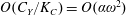 $O(C_{Y}/K_{C})=O(\unicode[STIX]{x1D6FC}\unicode[STIX]{x1D714}^{2})$
according to (5.5). Thus, the shear reconfiguration number is
$O(C_{Y}/K_{C})=O(\unicode[STIX]{x1D6FC}\unicode[STIX]{x1D714}^{2})$
according to (5.5). Thus, the shear reconfiguration number is
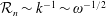 ${\mathcal{R}}_{n}\sim k^{-1}\sim \unicode[STIX]{x1D714}^{-1/2}$
, which is consistent with the slope observed in figure 9(a).
${\mathcal{R}}_{n}\sim k^{-1}\sim \unicode[STIX]{x1D714}^{-1/2}$
, which is consistent with the slope observed in figure 9(a).
As shown in figure 9(b), the location
 $s_{n}$
along the span of the blade where the maximum shear stress
$s_{n}$
along the span of the blade where the maximum shear stress
 $\max (\unicode[STIX]{x1D70E}_{n})$
is reached varies with the frequency. In the rigid domain
$\max (\unicode[STIX]{x1D70E}_{n})$
is reached varies with the frequency. In the rigid domain
 $\unicode[STIX]{x1D714}<1$
the maximum stress remains at the clamped edge, until the first resonance is reached. After
$\unicode[STIX]{x1D714}<1$
the maximum stress remains at the clamped edge, until the first resonance is reached. After
 $\unicode[STIX]{x1D714}_{1}$
, the maximum stress starts moving from the clamped edge towards the free tip as
$\unicode[STIX]{x1D714}_{1}$
, the maximum stress starts moving from the clamped edge towards the free tip as
 ${\mathcal{R}}_{n}$
decreases, before suddenly going back to the clamping point as
${\mathcal{R}}_{n}$
decreases, before suddenly going back to the clamping point as
 ${\mathcal{R}}_{n}$
starts increasing again, until the second resonance is attained. Similarly, after
${\mathcal{R}}_{n}$
starts increasing again, until the second resonance is attained. Similarly, after
 $\unicode[STIX]{x1D714}_{2}$
, the locus moves again as
$\unicode[STIX]{x1D714}_{2}$
, the locus moves again as
 ${\mathcal{R}}_{n}$
decreases and then comes back as
${\mathcal{R}}_{n}$
decreases and then comes back as
 ${\mathcal{R}}_{n}$
starts increasing towards the next resonance, and so on. This trajectory of the most solicited spot is independent of
${\mathcal{R}}_{n}$
starts increasing towards the next resonance, and so on. This trajectory of the most solicited spot is independent of
 $K_{C}$
, except close to the transition towards the convective regime. Indeed, for
$K_{C}$
, except close to the transition towards the convective regime. Indeed, for
 $K_{C}=1$
, the maximum shear stress remains at the clamping point for any value of the frequency ratio.
$K_{C}=1$
, the maximum shear stress remains at the clamping point for any value of the frequency ratio.
In the convective regime
 $K_{C}>1$
, we have shown that all the curvature concentrates within an elastic boundary layer of typical size
$K_{C}>1$
, we have shown that all the curvature concentrates within an elastic boundary layer of typical size
 $\unicode[STIX]{x1D6FF}=(K_{C}\,\unicode[STIX]{x1D714}^{2})^{-1/4}$
close to the attachment point. Consequently, the location of the maximum stress is always located at the clamping point in the convective regime. Besides, the variations of the shear reconfiguration number
$\unicode[STIX]{x1D6FF}=(K_{C}\,\unicode[STIX]{x1D714}^{2})^{-1/4}$
close to the attachment point. Consequently, the location of the maximum stress is always located at the clamping point in the convective regime. Besides, the variations of the shear reconfiguration number
 ${\mathcal{R}}_{n}$
, displayed as a function of the frequency ratio in figure 10(a), all collapse on the same curve when replotted as a function of
${\mathcal{R}}_{n}$
, displayed as a function of the frequency ratio in figure 10(a), all collapse on the same curve when replotted as a function of
 $K_{C}\,\unicode[STIX]{x1D714}^{2}$
in figure 10(b). Even the transition case
$K_{C}\,\unicode[STIX]{x1D714}^{2}$
in figure 10(b). Even the transition case
 $K_{C}=1$
also follows the same trend on average, but still exhibits some variations and small resonances due to the persistent modal nature of the response. When
$K_{C}=1$
also follows the same trend on average, but still exhibits some variations and small resonances due to the persistent modal nature of the response. When
 $K_{C}\,\unicode[STIX]{x1D714}^{2}<1$
, the scale of the boundary layer exceeds the length of the structure so the blade behaves rigidly and
$K_{C}\,\unicode[STIX]{x1D714}^{2}<1$
, the scale of the boundary layer exceeds the length of the structure so the blade behaves rigidly and
 ${\mathcal{R}}_{n}\sim 1$
. Conversely when
${\mathcal{R}}_{n}\sim 1$
. Conversely when
 $K_{C}\,\unicode[STIX]{x1D714}^{2}>1$
, the motion allowed by the flexibility is responsible for an alleviation of the internal shear stress. We may estimate the slope of the asymptotic decay by a similar argument as in the modal regime. Assuming that the characteristic bending length scales as the boundary layer thickness
$K_{C}\,\unicode[STIX]{x1D714}^{2}>1$
, the motion allowed by the flexibility is responsible for an alleviation of the internal shear stress. We may estimate the slope of the asymptotic decay by a similar argument as in the modal regime. Assuming that the characteristic bending length scales as the boundary layer thickness
 $\unicode[STIX]{x1D6FF}$
, we now have
$\unicode[STIX]{x1D6FF}$
, we now have
 $Q\sim O(\unicode[STIX]{x1D6FC}\times \unicode[STIX]{x1D6FF}^{-3})$
and the rigid shear force of order
$Q\sim O(\unicode[STIX]{x1D6FC}\times \unicode[STIX]{x1D6FF}^{-3})$
and the rigid shear force of order
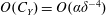 $O(C_{Y})=O(\unicode[STIX]{x1D6FC}\unicode[STIX]{x1D6FF}^{-4})$
. We thus obtain
$O(C_{Y})=O(\unicode[STIX]{x1D6FC}\unicode[STIX]{x1D6FF}^{-4})$
. We thus obtain
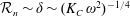 ${\mathcal{R}}_{n}\sim \unicode[STIX]{x1D6FF}\sim (K_{C}\,\unicode[STIX]{x1D714}^{2})^{-1/4}$
, in agreement with figure 10(b). Note that, as illustrated in figure 10(a), reconfiguration in the elastic boundary layer occurs even in the quasi-static regime
${\mathcal{R}}_{n}\sim \unicode[STIX]{x1D6FF}\sim (K_{C}\,\unicode[STIX]{x1D714}^{2})^{-1/4}$
, in agreement with figure 10(b). Note that, as illustrated in figure 10(a), reconfiguration in the elastic boundary layer occurs even in the quasi-static regime
 $\unicode[STIX]{x1D714}<1$
provided that
$\unicode[STIX]{x1D714}<1$
provided that
 $K_{C}\,\unicode[STIX]{x1D714}^{2}>1$
. Indeed, in this particular case, the rigid force
$K_{C}\,\unicode[STIX]{x1D714}^{2}>1$
. Indeed, in this particular case, the rigid force
 $q_{rigid}$
that appears on the right-hand side of the small-amplitude static equation (4.2) would actually lead to static deformations exceeding the excursion of the fluid particles. This is not possible in this drag-dominated regime as only strong inertial forces can cause the structure to overshoot the fluid particles. The drag term of (4.3) thus ensures the limitation of the structural excursion to that of the fluid particles, while only the elastic boundary layer that develops close to the clamped edge actually satisfies the quasi-static equilibrium between the elasticity forces and the drag (which amounts to neglecting the
$q_{rigid}$
that appears on the right-hand side of the small-amplitude static equation (4.2) would actually lead to static deformations exceeding the excursion of the fluid particles. This is not possible in this drag-dominated regime as only strong inertial forces can cause the structure to overshoot the fluid particles. The drag term of (4.3) thus ensures the limitation of the structural excursion to that of the fluid particles, while only the elastic boundary layer that develops close to the clamped edge actually satisfies the quasi-static equilibrium between the elasticity forces and the drag (which amounts to neglecting the
 $\dot{\tilde{x}}$
terms in the boundary layer equation (4.5)). Consequently, the scaling of the drag associated with reconfiguration in the elastic boundary layer remains valid in this domain as well.
$\dot{\tilde{x}}$
terms in the boundary layer equation (4.5)). Consequently, the scaling of the drag associated with reconfiguration in the elastic boundary layer remains valid in this domain as well.

Figure 10. Shear reconfiguration number in the convective regime against (a) the frequency ratio
 $\unicode[STIX]{x1D714}$
, (b) the rescaled parameter
$\unicode[STIX]{x1D714}$
, (b) the rescaled parameter
 $K_{C}\,\unicode[STIX]{x1D714}^{2}$
, for
$K_{C}\,\unicode[STIX]{x1D714}^{2}$
, for
 $K_{C}=10^{0}$
(– – –),
$K_{C}=10^{0}$
(– – –),
 $K_{C}=10^{1}$
(— ⋅ —),
$K_{C}=10^{1}$
(— ⋅ —),
 $K_{C}=10^{2}$
(——).
$K_{C}=10^{2}$
(——).
5.4 Large amplitude of flow oscillation
$\unicode[STIX]{x1D6FC}=A/L\gg 1$

In the large-amplitude regime (
 $\unicode[STIX]{x1D6FC}>1$
), we have proven that significant structural motion may only occur during a short period of time
$\unicode[STIX]{x1D6FC}>1$
), we have proven that significant structural motion may only occur during a short period of time
 $T_{r}$
following flow reversal (
$T_{r}$
following flow reversal (
 $\unicode[STIX]{x1D714}t=0$
). During that time, the flow magnitude is close to zero and the drag force is at its minimum. Drag being the dominant term of the equation, we expect the largest stress to be experienced when it is at its maximum around
$\unicode[STIX]{x1D714}t=0$
). During that time, the flow magnitude is close to zero and the drag force is at its minimum. Drag being the dominant term of the equation, we expect the largest stress to be experienced when it is at its maximum around
 $\unicode[STIX]{x1D714}t=\pm \unicode[STIX]{x03C0}/2$
, at a time where the structure is in quasi-static equilibrium with the flow forces. Besides, the flow acceleration cancels out when the flow magnitude is maximum so that, at the time where the stress peaks, equation (2.8) reduces to the static equation
$\unicode[STIX]{x1D714}t=\pm \unicode[STIX]{x03C0}/2$
, at a time where the structure is in quasi-static equilibrium with the flow forces. Besides, the flow acceleration cancels out when the flow magnitude is maximum so that, at the time where the stress peaks, equation (2.8) reduces to the static equation
 $$\begin{eqnarray}\displaystyle \unicode[STIX]{x1D705}^{\prime \prime }+\frac{1}{2}\unicode[STIX]{x1D705}^{3}-C_{Y}\left[|\text{cos}\,\unicode[STIX]{x1D703}|\cos \unicode[STIX]{x1D703}-\frac{1}{\unicode[STIX]{x1D706}}\unicode[STIX]{x1D705}\left(\sin ^{2}\unicode[STIX]{x1D703}-\frac{1}{2}\cos ^{2}\unicode[STIX]{x1D703}\right)\right]=0. & & \displaystyle\end{eqnarray}$$
In the quasi-static part of the cycle, the amplitude and frequency parameter influence the shape of the structure and the internal stress only through the Cauchy number
 $C_{Y}=\unicode[STIX]{x1D706}\unicode[STIX]{x1D6FC}^{2}\unicode[STIX]{x1D714}^{2}$
. Consequently, the evolution of the shear reconfiguration number shown in figure 11(a) as a function of the frequency ratio
$C_{Y}=\unicode[STIX]{x1D706}\unicode[STIX]{x1D6FC}^{2}\unicode[STIX]{x1D714}^{2}$
. Consequently, the evolution of the shear reconfiguration number shown in figure 11(a) as a function of the frequency ratio
 $\unicode[STIX]{x1D714}$
(for
$\unicode[STIX]{x1D714}$
(for
 $\unicode[STIX]{x1D706}=12.7$
) collapse very well on the static curve obtained with (5.6) when replotted as a function of the Cauchy number in figure 11(b). The curves are perfectly superimposed for
$\unicode[STIX]{x1D706}=12.7$
) collapse very well on the static curve obtained with (5.6) when replotted as a function of the Cauchy number in figure 11(b). The curves are perfectly superimposed for
 $\unicode[STIX]{x1D6FC}=10$
, but even for
$\unicode[STIX]{x1D6FC}=10$
, but even for
 $\unicode[STIX]{x1D6FC}$
as small as 1, agreement is already very good. When the Cauchy number is less than 1, deflection is negligible so (5.6) actually reduces to the small-amplitude static equation (4.2). In this limit, even though the amplitude of the forcing is large
$\unicode[STIX]{x1D6FC}$
as small as 1, agreement is already very good. When the Cauchy number is less than 1, deflection is negligible so (5.6) actually reduces to the small-amplitude static equation (4.2). In this limit, even though the amplitude of the forcing is large
 $\unicode[STIX]{x1D6FC}>1$
, we actually recover the small-amplitude static regime in which the structure experiences the same amount of stress as if it were rigid
$\unicode[STIX]{x1D6FC}>1$
, we actually recover the small-amplitude static regime in which the structure experiences the same amount of stress as if it were rigid
 ${\mathcal{R}}_{n}\sim 1$
.
${\mathcal{R}}_{n}\sim 1$
.
On the other hand, when the Cauchy number is large
 $C_{Y}>1$
, the stress is much reduced. In the limit where drag dominates over the added mass corrective term (limit of infinite slenderness
$C_{Y}>1$
, the stress is much reduced. In the limit where drag dominates over the added mass corrective term (limit of infinite slenderness
 $\unicode[STIX]{x1D706}\rightarrow \infty$
), the static equation (5.6) has a self-similar structure. The scaling of the terms of the equation provides the length of the self-similar boundary layer
$\unicode[STIX]{x1D706}\rightarrow \infty$
), the static equation (5.6) has a self-similar structure. The scaling of the terms of the equation provides the length of the self-similar boundary layer
 $\ell _{s}=C_{Y}^{-1/3}$
within which all the curvature concentrates. Consequently we may here again estimate the asymptotic behaviour of the shear reconfiguration number by a scaling argument. In this case, the saturated angle
$\ell _{s}=C_{Y}^{-1/3}$
within which all the curvature concentrates. Consequently we may here again estimate the asymptotic behaviour of the shear reconfiguration number by a scaling argument. In this case, the saturated angle
 $\unicode[STIX]{x1D703}$
is of order
$\unicode[STIX]{x1D703}$
is of order
 $O(1)$
so the shear force
$O(1)$
so the shear force
 $Q=\unicode[STIX]{x1D705}^{\prime }\sim O(1\times \ell _{s}^{-2})$
. The rigid shear force is of order
$Q=\unicode[STIX]{x1D705}^{\prime }\sim O(1\times \ell _{s}^{-2})$
. The rigid shear force is of order
 $O(C_{Y})=O(\ell _{s}^{-3})$
so we get
$O(C_{Y})=O(\ell _{s}^{-3})$
so we get
 ${\mathcal{R}}_{n}\sim \ell _{s}\sim C_{Y}^{-1/3}$
. The slope in figure 11(b) is close but differs slightly from that estimation. The analysis of appendix B shows that this discrepancy is due to the rather small value of
${\mathcal{R}}_{n}\sim \ell _{s}\sim C_{Y}^{-1/3}$
. The slope in figure 11(b) is close but differs slightly from that estimation. The analysis of appendix B shows that this discrepancy is due to the rather small value of
 $\unicode[STIX]{x1D706}=12.7$
. For any larger slenderness, the asymptotic scaling provided here matches very well the numerical results. Note that this bending length is similar to that previously found by Gosselin et al. (Reference Gosselin, de Langre and Machado-Almeida2010) who neglected the cubic term in curvature in their governing equation, as well as that found by Alben et al. (Reference Alben, Shelley and Zhang2004) for the case of a two-dimensional plate (opposite limit of infinite width). The extended validity of this static bending length to the case of large-amplitude unsteady flows was moreover suggested in Luhar & Nepf (Reference Luhar and Nepf2016).
$\unicode[STIX]{x1D706}=12.7$
. For any larger slenderness, the asymptotic scaling provided here matches very well the numerical results. Note that this bending length is similar to that previously found by Gosselin et al. (Reference Gosselin, de Langre and Machado-Almeida2010) who neglected the cubic term in curvature in their governing equation, as well as that found by Alben et al. (Reference Alben, Shelley and Zhang2004) for the case of a two-dimensional plate (opposite limit of infinite width). The extended validity of this static bending length to the case of large-amplitude unsteady flows was moreover suggested in Luhar & Nepf (Reference Luhar and Nepf2016).
Note finally that this analysis is independent of the magnitude of the reversal time
 $T_{r}$
. The key point of this analysis lies in the fact that even if significant dynamics may be involved during reversal when
$T_{r}$
. The key point of this analysis lies in the fact that even if significant dynamics may be involved during reversal when
 $T_{r}\gg 1$
, the maximum stress is endured at a time when the structure is in static equilibrium with the fluid forces. This remains obviously true when
$T_{r}\gg 1$
, the maximum stress is endured at a time when the structure is in static equilibrium with the fluid forces. This remains obviously true when
 $T_{r}\ll 1$
and static equilibrium is enforced at all times.
$T_{r}\ll 1$
and static equilibrium is enforced at all times.
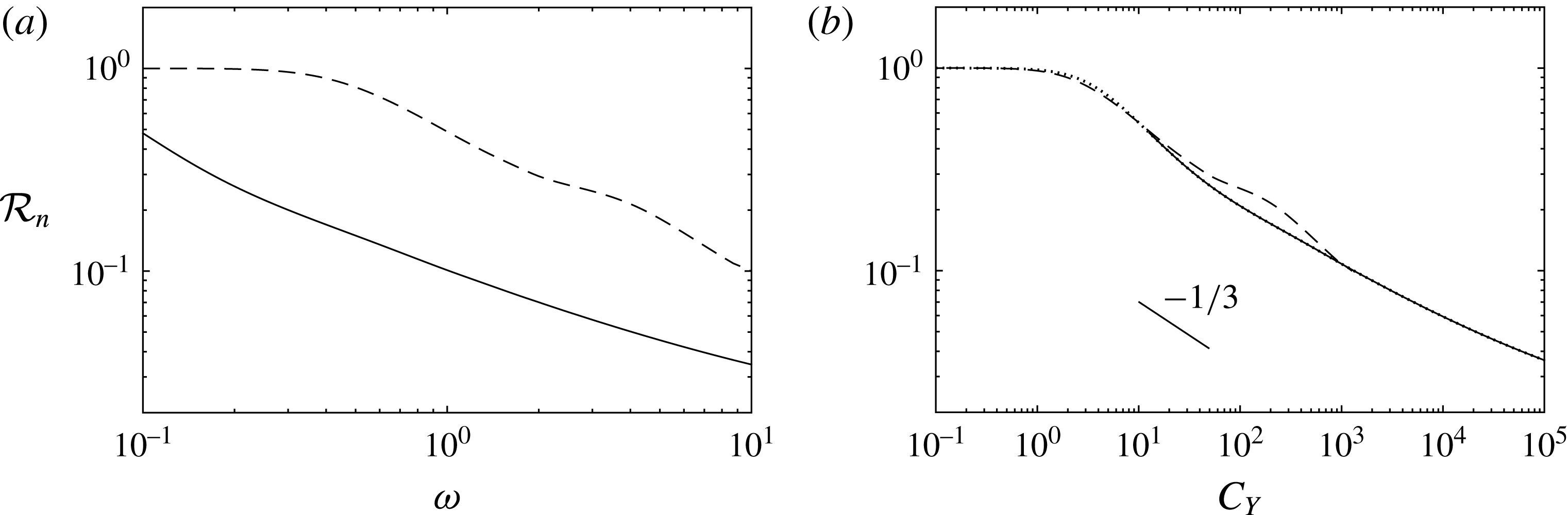
Figure 11. Shear reconfiguration number in the large-amplitude regime for
 $\unicode[STIX]{x1D706}=12.7$
, against (a) the frequency ratio
$\unicode[STIX]{x1D706}=12.7$
, against (a) the frequency ratio
 $\unicode[STIX]{x1D714}$
, (b) the Cauchy number
$\unicode[STIX]{x1D714}$
, (b) the Cauchy number
 $C_{Y}$
, for
$C_{Y}$
, for
 $\unicode[STIX]{x1D6FC}=10^{0}$
(– – –),
$\unicode[STIX]{x1D6FC}=10^{0}$
(– – –),
 $\unicode[STIX]{x1D6FC}=10^{1}$
(——). Static solution obtained with (5.6) (
$\unicode[STIX]{x1D6FC}=10^{1}$
(——). Static solution obtained with (5.6) (
 $\cdots \cdots$
, on (b) only).
$\cdots \cdots$
, on (b) only).
6 Discussion
6.1 Stress alleviation due to flexibility and bending length
Depending on the values of the amplitude and frequency of the oscillating flow, we have identified four distinct kinematic regimes summarized in figure 8. In each regime, the consequences of the flexibility on the magnitude of the internal stress are different. The varying scalings of the shear reconfiguration number
 ${\mathcal{R}}_{n}$
depending on the amplitude and frequency of the flow are schematically displayed in figure 12.
${\mathcal{R}}_{n}$
depending on the amplitude and frequency of the flow are schematically displayed in figure 12.

Figure 12. Schematic view of the reconfiguration regimes in the amplitude–frequency space.
As long as the forcing is dominated by the inertial forces (in the modal regime
 $A\ll W$
), there exists a risk of resonance if the frequency of the flow matches one of the natural frequencies of the structure. This is a case where the dynamical motion allowed by the flexibility may be responsible for a magnification of the internal stress. However, this is also the region in the parameter space where the loading is the lowest and so this is unlikely to cause any severe damage. Far from the resonances and in all other cases, flexibility always alleviates the magnitude of the internal stress.
$A\ll W$
), there exists a risk of resonance if the frequency of the flow matches one of the natural frequencies of the structure. This is a case where the dynamical motion allowed by the flexibility may be responsible for a magnification of the internal stress. However, this is also the region in the parameter space where the loading is the lowest and so this is unlikely to cause any severe damage. Far from the resonances and in all other cases, flexibility always alleviates the magnitude of the internal stress.
The general scaling of the reconfiguration numbers is related to some characteristic bending length
 $\ell _{b}$
such that
$\ell _{b}$
such that
 ${\mathcal{R}}_{n}\sim \ell _{b}$
and
${\mathcal{R}}_{n}\sim \ell _{b}$
and
 ${\mathcal{R}}_{\unicode[STIX]{x1D70F}}\sim \ell _{b}^{2}$
(see appendix A), but the scaling of that very bending length depends on the reconfiguration regime. In the modal regime (
${\mathcal{R}}_{\unicode[STIX]{x1D70F}}\sim \ell _{b}^{2}$
(see appendix A), but the scaling of that very bending length depends on the reconfiguration regime. In the modal regime (
 $A\ll W$
), the bending length is proportional to the wavelength of the dominant mode that varies as
$A\ll W$
), the bending length is proportional to the wavelength of the dominant mode that varies as
 $\ell _{b}=k^{-1}=\unicode[STIX]{x1D714}^{-1/2}$
. In the convective regime (
$\ell _{b}=k^{-1}=\unicode[STIX]{x1D714}^{-1/2}$
. In the convective regime (
 $W\ll A\ll L$
), curvature is confined in the elastic boundary layer so naturally
$W\ll A\ll L$
), curvature is confined in the elastic boundary layer so naturally
 $\ell _{b}=\unicode[STIX]{x1D6FF}=(\unicode[STIX]{x1D706}\unicode[STIX]{x1D6FC})^{-1/4}\unicode[STIX]{x1D714}^{-1/2}$
. The characteristic bending length varies continuously between the two small-amplitude regimes as their expressions are similar at the transition when
$\ell _{b}=\unicode[STIX]{x1D6FF}=(\unicode[STIX]{x1D706}\unicode[STIX]{x1D6FC})^{-1/4}\unicode[STIX]{x1D714}^{-1/2}$
. The characteristic bending length varies continuously between the two small-amplitude regimes as their expressions are similar at the transition when
 $K_{C}=\unicode[STIX]{x1D706}\unicode[STIX]{x1D6FC}=1$
. On the other hand, in the large-amplitude regime (
$K_{C}=\unicode[STIX]{x1D706}\unicode[STIX]{x1D6FC}=1$
. On the other hand, in the large-amplitude regime (
 $A\gg L$
) the bending length transitions to
$A\gg L$
) the bending length transitions to
 $\ell _{b}=\ell _{s}=C_{Y}^{-1/3}=(\unicode[STIX]{x1D706}\unicode[STIX]{x1D6FC}^{2}\unicode[STIX]{x1D714}^{2})^{-1/3}$
. The boundary of the rigid domain with the three different reconfiguration regimes is nonetheless continuous as illustrated in figure 12.
$\ell _{b}=\ell _{s}=C_{Y}^{-1/3}=(\unicode[STIX]{x1D706}\unicode[STIX]{x1D6FC}^{2}\unicode[STIX]{x1D714}^{2})^{-1/3}$
. The boundary of the rigid domain with the three different reconfiguration regimes is nonetheless continuous as illustrated in figure 12.
6.2 Consequences in terms of growth pattern of aquatic flexible plants
In any of the three reconfiguration regimes, the reconfiguration numbers scale in dimensional form with the length of the blade as
 ${\mathcal{R}}_{n}\sim L^{-1}$
and
${\mathcal{R}}_{n}\sim L^{-1}$
and
 ${\mathcal{R}}_{\unicode[STIX]{x1D70F}}\sim L^{-2}$
. Given the scalings of the rigid loads and of the internal stresses in § 5.1, we thus obtain the cancellation of the dependency of the dimensional forces and internal stresses on the actual length of the blade
${\mathcal{R}}_{\unicode[STIX]{x1D70F}}\sim L^{-2}$
. Given the scalings of the rigid loads and of the internal stresses in § 5.1, we thus obtain the cancellation of the dependency of the dimensional forces and internal stresses on the actual length of the blade
 $\unicode[STIX]{x1D70E}_{n}\propto Q\sim L^{0}$
and
$\unicode[STIX]{x1D70E}_{n}\propto Q\sim L^{0}$
and
 $\unicode[STIX]{x1D70E}_{\unicode[STIX]{x1D70F}}\propto M\sim L^{0}$
. This loss of relevance of the true length of the structure in aid of a smaller characteristic bending length was already pointed out in the steady case (see de Langre, Gutierrez & Cossé Reference de Langre, Gutierrez and Cossé2012) and remains valid in the oscillatory case. Consequently, it does not seem as if there is any mechanical limit to size in wave-swept flexible kelps, as long as growth is concentrated in the axial direction.
$\unicode[STIX]{x1D70E}_{\unicode[STIX]{x1D70F}}\propto M\sim L^{0}$
. This loss of relevance of the true length of the structure in aid of a smaller characteristic bending length was already pointed out in the steady case (see de Langre, Gutierrez & Cossé Reference de Langre, Gutierrez and Cossé2012) and remains valid in the oscillatory case. Consequently, it does not seem as if there is any mechanical limit to size in wave-swept flexible kelps, as long as growth is concentrated in the axial direction.
But real plants grow according to more complex allometric patterns (Denny & Cowen Reference Denny and Cowen1997; Gaylord & Denny Reference Gaylord and Denny1997). Following the growth of a plant in the variables of figure 12 amounts to decreasing
 $\unicode[STIX]{x1D6FC}$
from the top. In the static reconfiguration regime, the internal stresses
$\unicode[STIX]{x1D6FC}$
from the top. In the static reconfiguration regime, the internal stresses
 $\unicode[STIX]{x1D70E}_{n}$
and
$\unicode[STIX]{x1D70E}_{n}$
and
 $\unicode[STIX]{x1D70E}_{\unicode[STIX]{x1D70F}}$
are both independent of any of the three dimensions
$\unicode[STIX]{x1D70E}_{\unicode[STIX]{x1D70F}}$
are both independent of any of the three dimensions
 $D$
,
$D$
,
 $W$
,
$W$
,
 $L$
and so growth does not affect the magnitude of the stresses in a given environment, no matter the allometry of the plant. When the structure reaches the convective regime (
$L$
and so growth does not affect the magnitude of the stresses in a given environment, no matter the allometry of the plant. When the structure reaches the convective regime (
 $L\geqslant A$
), the stresses become decreasing functions of the thickness
$L\geqslant A$
), the stresses become decreasing functions of the thickness
 $D$
but remain independent of
$D$
but remain independent of
 $W$
and
$W$
and
 $L$
. One might think that a growth pattern favouring thickness would be advantageous, but this is only so for thin plates
$L$
. One might think that a growth pattern favouring thickness would be advantageous, but this is only so for thin plates
 $D<W$
for which the elastic effects are confined in the plane of the flow. A thicker structure might experience three-dimensional deformations that would make the dynamics considerably more complex. Finally, in the modal regime (
$D<W$
for which the elastic effects are confined in the plane of the flow. A thicker structure might experience three-dimensional deformations that would make the dynamics considerably more complex. Finally, in the modal regime (
 $W\geqslant A$
), the stresses now start increasing with the width
$W\geqslant A$
), the stresses now start increasing with the width
 $W$
, and the risk of resonances may enhance the stresses even more depending on the frequency of the flow. It thus appears detrimental for a flexible plant to grow in width in excess of the fluid particle excursion.
$W$
, and the risk of resonances may enhance the stresses even more depending on the frequency of the flow. It thus appears detrimental for a flexible plant to grow in width in excess of the fluid particle excursion.
These remarks come as complementary answers to the work of Koehl (Reference Koehl1984) and especially Denny et al. (Reference Denny, Daniel and Koehl1985), Gaylord, Blanchette & Denny (Reference Gaylord, Blanchette and Denny1994) and Denny (Reference Denny1999). Koehl (Reference Koehl1984) first noted that ‘flexibility in combination with great length provides a mechanism of avoiding bearing large forces in habitats subjected to oscillating flow’, in comparison to rigid organisms that need to remain small. However the question of whether there might be size limits imposed on wave-swept flexible organisms due to the oscillatory fluid loading has never received a definitive answer. Our results indicate that for slender, neutrally buoyant blades, the hydrodynamic loads do limit the width, but put no constraints on the axial growth.
6.3 Remarks on previous work about the convective regime
Most aquatic plants are close to neutrally buoyant and the horizontal amplitude of the passing waves is typically much larger than the width if not the length of these plants (see Gaylord et al.
Reference Gaylord, Blanchette and Denny1994; Denny & Cowen Reference Denny and Cowen1997; Gaylord & Denny Reference Gaylord and Denny1997). Thus it seems that plants growing larger than the fluid particles excursion are likely to remain in the convective regime in order to avoid large flow-induced stresses. The work of Mullarney & Henderson (Reference Mullarney and Henderson2010) and Luhar & Nepf (Reference Luhar and Nepf2016) has focused mainly on this convective regime. The latter show on their figure 11 that their effective length (analogous to our normal reconfiguration number
 ${\mathcal{R}}_{n}$
) seems to scale as
${\mathcal{R}}_{n}$
) seems to scale as
 $(C_{Y}/\unicode[STIX]{x1D6FC})^{-1/4}=(\unicode[STIX]{x1D706}\unicode[STIX]{x1D6FC}\unicode[STIX]{x1D714}^{2})^{-1/4}=\unicode[STIX]{x1D6FF}$
. This result is consistent with the scaling of the elastic boundary layer that develops in the convective regime, and indeed almost all the experimental cases of Luhar & Nepf (Reference Luhar and Nepf2016) were obtained within the appropriate range
$(C_{Y}/\unicode[STIX]{x1D6FC})^{-1/4}=(\unicode[STIX]{x1D706}\unicode[STIX]{x1D6FC}\unicode[STIX]{x1D714}^{2})^{-1/4}=\unicode[STIX]{x1D6FF}$
. This result is consistent with the scaling of the elastic boundary layer that develops in the convective regime, and indeed almost all the experimental cases of Luhar & Nepf (Reference Luhar and Nepf2016) were obtained within the appropriate range
 $\unicode[STIX]{x1D6FC}\leqslant 1$
and
$\unicode[STIX]{x1D6FC}\leqslant 1$
and
 $K_{C}\geqslant 1$
(more precisely
$K_{C}\geqslant 1$
(more precisely
 $0.06\leqslant \unicode[STIX]{x1D6FC}\leqslant 1.32$
and
$0.06\leqslant \unicode[STIX]{x1D6FC}\leqslant 1.32$
and
 $0.76\leqslant K_{C}\leqslant 4.2$
). However, because the slenderness parameter of their blades is rather low (between
$0.76\leqslant K_{C}\leqslant 4.2$
). However, because the slenderness parameter of their blades is rather low (between
 $\unicode[STIX]{x1D706}=3.2$
and
$\unicode[STIX]{x1D706}=3.2$
and
 $\unicode[STIX]{x1D706}=12.7$
),
$\unicode[STIX]{x1D706}=12.7$
),
 $\unicode[STIX]{x1D6FC}$
and
$\unicode[STIX]{x1D6FC}$
and
 $K_{C}$
are quite close to each other and consequently most of their points are very close to either one of the boundaries of that regime. Some particular points in that study show an increase of the load compared to the rigid case. The authors suggested that this might result from an interaction between the blade and the vortex shed at the tip. But these points are characterized by a rather small amplitude
$K_{C}$
are quite close to each other and consequently most of their points are very close to either one of the boundaries of that regime. Some particular points in that study show an increase of the load compared to the rigid case. The authors suggested that this might result from an interaction between the blade and the vortex shed at the tip. But these points are characterized by a rather small amplitude
 $\unicode[STIX]{x1D6FC}=O(10^{-1})$
and Keulegan–Carpenter number
$\unicode[STIX]{x1D6FC}=O(10^{-1})$
and Keulegan–Carpenter number
 $K_{C}\sim 0.7-1.2$
, and forcing frequencies close to the resonance frequency
$K_{C}\sim 0.7-1.2$
, and forcing frequencies close to the resonance frequency
 $\unicode[STIX]{x1D714}\sim 1-5$
. For instance, the largest load was obtained for (
$\unicode[STIX]{x1D714}\sim 1-5$
. For instance, the largest load was obtained for (
 $\unicode[STIX]{x1D6FC}=0.12$
,
$\unicode[STIX]{x1D6FC}=0.12$
,
 $K_{C}=0.76$
and
$K_{C}=0.76$
and
 $\unicode[STIX]{x1D714}=2.30$
). It is thus a possibility that the load enhancement is simply the consequence of a resonance of the impinging wave with the first natural mode of the structure, due to the persistent modal nature of the dynamic response for such values of the parameters. Conversely, other points obtained for
$\unicode[STIX]{x1D714}=2.30$
). It is thus a possibility that the load enhancement is simply the consequence of a resonance of the impinging wave with the first natural mode of the structure, due to the persistent modal nature of the dynamic response for such values of the parameters. Conversely, other points obtained for
 $\unicode[STIX]{x1D6FC}=O(1)$
seem to collapse quite well with the others. We have shown that for such high values of the amplitude parameter, at least when
$\unicode[STIX]{x1D6FC}=O(1)$
seem to collapse quite well with the others. We have shown that for such high values of the amplitude parameter, at least when
 $\unicode[STIX]{x1D706}=12.7$
, the reconfiguration number should be close to its static equivalent. But if very slender structures exhibit a clear asymptotic regime
$\unicode[STIX]{x1D706}=12.7$
, the reconfiguration number should be close to its static equivalent. But if very slender structures exhibit a clear asymptotic regime
 ${\mathcal{R}}_{n}\sim C_{Y}^{-1/3}$
, decreasing the slenderness below
${\mathcal{R}}_{n}\sim C_{Y}^{-1/3}$
, decreasing the slenderness below
 $O(10)$
mitigates the efficiency of the reconfiguration and increases the slope so that it may be difficult to know the difference with the scaling of the convective regime.
$O(10)$
mitigates the efficiency of the reconfiguration and increases the slope so that it may be difficult to know the difference with the scaling of the convective regime.
6.4 Limits and extensions of the model
In all this study we have focused exclusively on the case of an infinitely thin, neutrally buoyant blade. These two assumptions have allowed us to neglect both the displaced mass and the structural mass. In practice however, aquatic plants are not strictly speaking of the same density as the water and their thicknesses might not be negligible.
First, if the thickness of the neutrally buoyant blade is not negligible anymore, we need to consider the inertial and virtual buoyancy forces. These forces might be responsible for additional inertial effects in the large-amplitude regime, such as persistent oscillations following the quick reversal with
 $T_{r}<1$
, or a flutter instability similar to that observed on axial flags. The dynamics induced would then be responsible for additional loads that may challenge the findings of that study. However, we expect the consequences to remain marginal, as damping by the drag term would still dominate. This is even more so as the slenderness is increased and for infinite slenderness, we do not expect any significant discrepancy with the present work. Besides, the small-amplitude regimes would not be affected in any way as (4.1) would remain the same, providing that the characteristic time of the structure used for non-dimensionalization is redefined to account for the structural mass
$T_{r}<1$
, or a flutter instability similar to that observed on axial flags. The dynamics induced would then be responsible for additional loads that may challenge the findings of that study. However, we expect the consequences to remain marginal, as damping by the drag term would still dominate. This is even more so as the slenderness is increased and for infinite slenderness, we do not expect any significant discrepancy with the present work. Besides, the small-amplitude regimes would not be affected in any way as (4.1) would remain the same, providing that the characteristic time of the structure used for non-dimensionalization is redefined to account for the structural mass
 $T_{s}=L^{2}\sqrt{(m_{a}+m)/EI}$
.
$T_{s}=L^{2}\sqrt{(m_{a}+m)/EI}$
.
If the structure is now lighter than the fluid, then its inertia is even more negligible. Buoyancy may still modify our results, but this effect should become negligible as soon as the fluid loading is dominant as explained in Luhar & Nepf (Reference Luhar and Nepf2011) and Luhar & Nepf (Reference Luhar and Nepf2016).
On the other hand, if the structure is much denser than the fluid, some more complicated dynamical effects might come into play due to the large structural inertia possibly overcoming even drag. We do not expect the conclusions of the present work to hold in that case.
7 Conclusion
This work provides a dynamical extension of the theory of reconfiguration to the case of oscillatory flow. Focusing on neutrally buoyant cantilever slender blades, we proved that flexibility is always favourable to reducing the internal stresses as long as drag dominates the fluid inertial forces. In fact, drag appears as the motor of reconfiguration. In large-amplitude oscillations (or equivalently in steady flow), drag is responsible for the static deflection that reduces the stress. In small-amplitude oscillations, it is also the saturation of the drag term that forces the passive convection of the structure with the fluid particles if the Keulegan–Carpenter number is large. Even in the less favourable case of small Keulegan–Carpenter numbers, it is the small drag term that saturates the resonances that occur due to the fluid inertia, even when the structural inertia is negligible. We also expect that drag would saturate flutter-like oscillations that might occur if the structural mass were not negligible, thus limiting the enhancement of the internal stresses to a bearable extent.

Figure 13. (a) Tensile reconfiguration number and (b) location of maximum tensile stress along the span in the modal regime, against the frequency ratio, for
 $K_{C}=10^{-2}$
(——),
$K_{C}=10^{-2}$
(——),
 $K_{C}=10^{-1}$
(— ⋅ —),
$K_{C}=10^{-1}$
(— ⋅ —),
 $K_{C}=10^{0}$
(– – –) and analytical solution for
$K_{C}=10^{0}$
(– – –) and analytical solution for
 $K_{C}\rightarrow 0$
(
$K_{C}\rightarrow 0$
(
 $\cdots \cdots$
). (c) Tensile reconfiguration number against
$\cdots \cdots$
). (c) Tensile reconfiguration number against
 $K_{C}\,\unicode[STIX]{x1D714}^{2}$
in the convective regime
$K_{C}\,\unicode[STIX]{x1D714}^{2}$
in the convective regime
 $K_{C}=10^{0}$
(– – –),
$K_{C}=10^{0}$
(– – –),
 $K_{C}=10^{1}$
(— ⋅ —),
$K_{C}=10^{1}$
(— ⋅ —),
 $K_{C}=10^{2}$
(——). (d) Tensile reconfiguration number in the large-amplitude regime for
$K_{C}=10^{2}$
(——). (d) Tensile reconfiguration number in the large-amplitude regime for
 $\unicode[STIX]{x1D706}=12.7$
, against the Cauchy number
$\unicode[STIX]{x1D706}=12.7$
, against the Cauchy number
 $C_{Y}$
for
$C_{Y}$
for
 $\unicode[STIX]{x1D6FC}=10^{0}$
(– – –),
$\unicode[STIX]{x1D6FC}=10^{0}$
(– – –),
 $\unicode[STIX]{x1D6FC}=10^{1}$
(——) and static solution obtained with (5.6) (
$\unicode[STIX]{x1D6FC}=10^{1}$
(——) and static solution obtained with (5.6) (
 $\cdots \cdots$
).
$\cdots \cdots$
).
As in the static case, we have shown that dynamic reconfiguration results in the concentration of the stresses on a short bending length near the clamped edge, only the scaling of that bending length varies depending on the dynamic regime. Consequently, the dependency of the internal stresses on the actual length of the structure disappears, and there does not seem to be any mechanical limitation to the axial growth of plants living in wave-swept environment due to the hydrodynamic loads. However, in order to avoid deleterious inertial effects, it seems better to keep a much smaller width than the excursion of the fluid particles. In other words, if there is no limitations to growth in itself, there is an incentive to grow slender based on mechanical considerations. Of course, the actual growth pattern of aquatic plants also involves other aspects such as the optimization of its biological functions that we do not take into account here.
Up to here, only the inertia of the fluid has been accounted for. We expect the inclusion of significant structural inertia should considerably modify the results of the present work.
Acknowledgements
The authors would like to acknowledge financial support from the DGA/DSTL grant 2014.60.0005 and fruitful discussions with N. Peake from DAMTP, Cambridge, UK.
Appendix A. Tensile stress
Similarly to the shear reconfiguration number, the variations of the tensile reconfiguration number are displayed in figure 13(a) for the modal regime, along with the location of the maximum stress in figure 13(b). Figures 13(c) and 13(d) respectively show the results in the convective and large-amplitude regime. All the conclusions drawn about the shear reconfiguration number are still valid for the tensile number. The only noticeable difference is the asymptotic scaling for large loadings. Indeed, the non-dimensional bending moment
 $M=\unicode[STIX]{x1D705}$
involves one less derivative in space than the shear force
$M=\unicode[STIX]{x1D705}$
involves one less derivative in space than the shear force
 $Q$
so that
$Q$
so that
 $M\sim Q\times \ell _{b}$
, while the non-dimensional rigid load is unchanged. Therefore,
$M\sim Q\times \ell _{b}$
, while the non-dimensional rigid load is unchanged. Therefore,
 ${\mathcal{R}}_{\unicode[STIX]{x1D70F}}\sim {\mathcal{R}}_{n}\times \ell _{b}\sim \ell _{b}^{2}$
. Finally, this provides
${\mathcal{R}}_{\unicode[STIX]{x1D70F}}\sim {\mathcal{R}}_{n}\times \ell _{b}\sim \ell _{b}^{2}$
. Finally, this provides
 ${\mathcal{R}}_{\unicode[STIX]{x1D70F}}\sim \unicode[STIX]{x1D714}^{-1}$
in the modal regime,
${\mathcal{R}}_{\unicode[STIX]{x1D70F}}\sim \unicode[STIX]{x1D714}^{-1}$
in the modal regime,
 ${\mathcal{R}}_{\unicode[STIX]{x1D70F}}\sim (K_{C}\,\unicode[STIX]{x1D714}^{2})^{-1/2}$
in the convective regime and
${\mathcal{R}}_{\unicode[STIX]{x1D70F}}\sim (K_{C}\,\unicode[STIX]{x1D714}^{2})^{-1/2}$
in the convective regime and
 ${\mathcal{R}}_{\unicode[STIX]{x1D70F}}\sim C_{Y}^{-2/3}$
in the large-amplitude regime, in agreement with the results shown.
${\mathcal{R}}_{\unicode[STIX]{x1D70F}}\sim C_{Y}^{-2/3}$
in the large-amplitude regime, in agreement with the results shown.
Appendix B. Influence of the slenderness on the static reconfiguration
In the large-amplitude regime, most of the cycle is quasi-static and the system is well modelled by (5.6). The different static reconfiguration curves for varying slenderness parameters shown in figure 14 prove that the reconfiguration numbers converge on an asymptotic trend as the slenderness is increased. For any finite
 $\unicode[STIX]{x1D706}$
, the discrepancy with the asymptotic curve remains quite small for the shear stress, and almost completely imperceptible for the tensile stress. The asymptotic scaling provided in § 5 can therefore be used even for moderately large slenderness.
$\unicode[STIX]{x1D706}$
, the discrepancy with the asymptotic curve remains quite small for the shear stress, and almost completely imperceptible for the tensile stress. The asymptotic scaling provided in § 5 can therefore be used even for moderately large slenderness.

Figure 14. Variations of the static reconfiguration numbers obtained with (5.6) ((a) shear, (b) tensile) as a function of the Cauchy number
 $C_{Y}$
, for
$C_{Y}$
, for
 $\unicode[STIX]{x1D706}=12.7$
(——),
$\unicode[STIX]{x1D706}=12.7$
(——),
 $\unicode[STIX]{x1D706}=127$
(– – –),
$\unicode[STIX]{x1D706}=127$
(– – –),
 $\unicode[STIX]{x1D706}=1270$
(
$\unicode[STIX]{x1D706}=1270$
(
 $\cdots \cdots$
).
$\cdots \cdots$
).


