


1. Introduction
A fully developed Poiseuille flow regime with a pure diffusive miscible interface arises when a more-viscous fluid displaces another miscible fluid with less viscosity in a channel. Such a stable pattern is termed as a ‘pure-Poiseuille-diffusive’ finger (Mishra, De Wit & Sahu Reference Mishra, De Wit and Sahu2012). This stable displacement flow has been studied experimentally by Balasubramaniam et al. (Reference Balasubramaniam, Rashidnia, Maxworthy and Kuang2005), Rashindia, Balasubramanium & Schrder (Reference Rashindia, Balasubramanium and Schrder2004) and Etrati & Frigaard (Reference Etrati and Frigaard2018), in a vertical cylindrical tube. The asymmetric sinuous-shaped unstable interface separating the fluids is found when the flow is in the downward direction. At the same time, at a higher displacement speed, an axisymmetric finger with a needle-shaped spike propagates out from the main fingertip when the flow is against gravity. To the best of our knowledge, these are the only experiments that have discussed the displacement flow in a classically stable system. Numerically, Mishra et al. (Reference Mishra, De Wit and Sahu2012) showed that this classically stable situation could be destabilized when the fluids have different diffusivity and more discussions on such effects are presented in a review article by Govindarajan & Sahu (Reference Govindarajan and Sahu2014).
In the counterpart, i.e. when a less-viscous fluid pushes a more-viscous fluid, if the flow rate is high enough, then a needle-shaped spike at the tip of the finger can be observed, as was done by Lajeunesse et al. (Reference Lajeunesse, Martin, Rakotomalala, Salin and Yortsos1999), in a vertical Hele–Shaw cell. Similarly, when an elongated finger of less-viscous fluid penetrates into a more-viscous one in a channel or pipe, a velocity fluctuation generated by viscosity contrast can develop Kelvin–Helmholtz (K–H) instability type roll-ups (Sahu et al. Reference Sahu, Ding, Valluri and Matar2009a, Govindarajan & Sahu Reference Govindarajan and Sahu2014). Etrati & Frigaard (Reference Etrati and Frigaard2018) performed experiments in a vertical and inclined pipe, and compared the flow features, like averaged concentration profile and front velocities, with the numerical results.
Hence it is believed that in a non-reactive channel/pipe flow, hydrodynamic instability of fingering or K–H-type instability alongside the elongated finger occurs when a bulk of less-viscous fluid displaces a more-viscous fluid (Sahu et al. Reference Sahu, Ding, Valluri and Matar2009a; Etrati & Frigaard Reference Etrati and Frigaard2018). In particular, if the viscosity increases in the direction of propagation globally, then fingering and K–H instability are noticed. Alternatively, even when a bulk of more-viscous fluid displaces a less-viscous one, a local increase of viscosity in the direction of the flow by double-diffusive effects can lead to such instabilities (Mishra et al. Reference Mishra, De Wit and Sahu2012).
The effect of chemical reaction on interfacial instabilities has become a recent attraction for many researchers, as it can lead to alteration of density and viscosity of the fluids. Experimentally, the propagation of the miscible reactive front in the capillary tube (Nagatsu et al. Reference Nagatsu, Hosokawa, Kato, Tada and Ueda2008) and that of the autocatalytic reaction front in laminar flows (Leconte et al. Reference Leconte, Martin, Rakotomalala and Salin2002) have been studied. The difficulty of producing a locally varying viscosity to induce instability is eased by local changes in the molecular structure via a chemical reaction with complex structured fluids (Burghelea et al. Reference Burghelea, Wielage-Burchard, Frigaard, Martinez and Feng2007). Burghelea et al. (Reference Burghelea, Wielage-Burchard, Frigaard, Martinez and Feng2007) conducted three sets of experiments and arrived at the conclusion that the chemical reaction can be treated as a new tool for efficient mixing in microfluidic flows even at low Reynolds number. Also, an experimental investigation was carried out by Burghelea & Frigaard (Reference Burghelea and Frigaard2011), which revealed an instability triggered by a fast chemical reaction in a low-inertia parallel flow in a small channel. They focused on the transverse growth of mixed regions by controlling the initial interface position and the two fluids’ relative inflow. Nevertheless, the dispersion analysis of reactive flows (Reshadi & Saidi Reference Reshadi and Saidi2019; Taghizadeh, Valdés-Parada & Wood Reference Taghizadeh, Valdés-Parada and Wood2020) is an active area of research, which provides building blocks for understanding the complex instabilities in reactive pipe flows.
In the context of viscous fingering (VF) instability, experimentally, it has been shown (Nagatsu et al. Reference Nagatsu, Matsuda, Kato and Tada2007; Riolfo et al. Reference Riolfo, Nagatsu, Iwata, Maes, Trevelyan and De Wit2012) that viscosity depends on the concentration of the solutes, and hence a chemical reaction can alter the viscosity gradient generating fingers at the fluid–fluid interface. They used the pH dependency of the viscous solutions of polymers (aqueous polyacrylic acid (PAA)) that undergo a ( $A+B \rightarrow C$)-type reaction, which tunes the changes in the gradient of the mobility profile. In the experiments by Nagatsu et al. (Reference Nagatsu, Matsuda, Kato and Tada2007) and Riolfo et al. (Reference Riolfo, Nagatsu, Iwata, Maes, Trevelyan and De Wit2012), both the displacing and the displaced fluid had different viscosity, while Podgorski et al. (Reference Podgorski, Sostarecz, Zorman and Belmonte2007) used the same viscosity bulk fluids that underwent a chemical reaction of (
 $A +B \rightarrow C$)-type producing a variety of fingering instabilities. In their experiments, they considered the aqueous solutions of the cationic surfactant cetyltrimethylammonium bromide (CTAB) and the organic salt sodium salicylate (NaSal). It was found that bringing CTAB and NaSal into contact produced a strongly viscoelastic micellar material, which caused a fingering instability at the underlying reactive interface. Subsequently, numerical studies on the reactive VF instability in both rectilinear (Gérard & De Wit Reference Gérard and De Wit2009) and radial (Sharma et al. Reference Sharma, Pramanik, Chen and Mishra2019) displacements in porous media have been performed. In these studies, the authors showed that reaction could induce VF-instability even if the underlying reactive fluids have the same viscosity. A considerable number of experimental studies of fingering instabilities by chemical reaction and numerical analysis in Darcy's regime is presented in a review article by De Wit (Reference De Wit2020). Also, De Wit (Reference De Wit2020) explicitly pointed out the lack of numerical analysis of chemohydrodynamic instabilities to date where Navier–Stokes equations govern the flow. Thus, a collective viewpoint from reactive experimental studies in the pipe flow and lack of numerical analysis of the chemohydrodynamic instabilities in the Navier–Stokes regime motivates the primary objective of this article.
Here, we investigate how the reaction destabilizes the pressure-driven channel flow even if the displacement is between two isoviscous fluids. Further, we investigate how the chemical reaction alters the viscosity profile in the channel flow that may cause interfacial instability. We numerically analyse these investigations and successfully explain the mechanism and onset dynamics of the instability. In comparison to the Darcy flow in a Hele–Shaw cell or Stokes flow in a capillary tube, the fundamental difficulty is in solving the coupled convection–diffusion–reaction (CDR) equations for reactant and product species with the Navier–Stokes equation in channel geometry. We have successfully overcome these challenges in numerical modelling by using a finite volume method that uses a fifth-order weighted essentially non-oscillatory (WENO) approximation for convection of solute concentrations. We find K–H-type billows at the fluid–fluid interface, which are formed due to the isothermal chemical reaction between two isoviscous fluids, and discuss the changes in their dynamical properties with respect to various governing flow parameters. An interesting scaling behaviour on the onset of instability is obtained, which shows proportionate dynamics with respect to  $Pe$, and the existence of a critical mobility ratio
  $R_c$ for obtaining the interfacial billows is revealed.
2. Mathematical formulation and numerical method
We consider the fluids containing the two reactants  $\textbf {A}$,
  $\textbf {B}$ and the product
  $\textbf {C}$ are miscible and Newtonian. We use a rectangular coordinate system
  $(x, y)$ to model the flow dynamics where
  $x$ and
  $y$ denote the horizontal and vertical coordinates, respectively. The rigid and impermeable channel walls are located at
  $y = 0$ and
  $y = L_y$, while its inlet and outlet coincide with
  $x = 0$ and
  $x = L_x$, respectively (figure 1). A solution of reactant
  $\textbf {A}$ with viscosity
  $\mu =\mu _{1}$ is injected at the channel inlet, along the
  $x$ direction, into a solution of reactant
  $\textbf {B}$ having the same viscosity
  $\mu _{1}$ with average velocity
  $Q/L_y$, where
  $Q$ denotes the total flow rate. Both reactants
  $\textbf {A}$ and
  $\textbf {B}$ are initially present in the same initial concentration
  $\varPhi _0$. A second-order chemical reaction
  $\textbf {A}+ \textbf {B} \xrightarrow {k} \textbf {C}$ takes place as soon as
  $\textbf {A}$ and
  $\textbf {B}$ are put in contact to yield a high-viscosity product
  $\textbf {C}$ with viscosity
  $\mu _{2}$ (
 $\mu _{2}> \mu _{1}$). The flow dynamics is governed by incompressible Navier–Stokes equations:
 \begin{gather} \boldsymbol{\nabla \cdot u} = 0, \end{gather}
 \begin{gather}\rho\left[ \frac{\partial \boldsymbol{u}}{\partial t} +\boldsymbol{u \cdot \nabla u} \right] ={-}\boldsymbol{\nabla} p + \boldsymbol{\nabla} \boldsymbol{\cdot} [\mu(c) (\boldsymbol{\nabla u}+ \boldsymbol{\nabla u}^{T}) ], \end{gather}
where  $\boldsymbol {u} = (u, v)$ is the velocity vector with components
  $u$ and
  $v$ in the
  $x$ and
  $y$ directions, respectively, and
  $p$ denotes pressure,
  $a,b,c$ denote the concentration of the two reactants
  $(\textbf {A},\textbf {B})$ and the product
  $\textbf {C}$, respectively, and they satisfy the following system of CDR equations:
 \begin{gather} \frac{\partial a}{\partial t} +\boldsymbol{u \cdot \nabla} a = D \nabla^{2} a-kab, \end{gather}
 \begin{gather}\frac{\partial b}{\partial t} +\boldsymbol{u \cdot \nabla} b = D \nabla^{2} b-kab, \end{gather}
 \begin{gather}\frac{\partial c}{\partial t} +\boldsymbol{u \cdot \nabla} c = D \nabla^{2} c+kab. \end{gather}
Figure 1. Schematic of the initial configuration.
We assume the same diffusion coefficient  $D$ of all the species
  $\textbf {A},\textbf {B}$ and
  $\textbf {C}$. Further it is assumed that the viscosity of the fluid varies exponentially with the product concentration as
  $\mu (c)=\mu _1 \,\textrm {e}^{ R_{c} c/\varPhi _0}$, where
  $R_c = \ln (\mu _{2}/\mu _{1})$.
2.1. Non-dimensionalization
We non-dimensionalize the equations using the characteristic length, time, velocity, pressure, viscosity and concentration as
 \begin{gather} (x,y) = L_{y}(\tilde{x},\tilde{y}), \quad t=\frac{L_{y}^{2}}{Q}\tilde{t}, \quad (u,v) = \frac{Q}{L_{y}}(\tilde{u}, \tilde{v}), \end{gather}
 \begin{gather}p = \frac{\rho Q^{2}}{L_{y}^{2}}\tilde{p}, \quad \mu = \tilde{\mu} \mu_1, \quad (\tilde{a}, \tilde{b}, \tilde{c}) = \frac{(a,b,c)}{\varPhi_{0}}, \end{gather}
where the tildes designate dimensionless quantities. After dropping tildes, the dimensionless governing equations become
 \begin{gather} \boldsymbol{\nabla \cdot u} = 0, \end{gather}
 \begin{gather}\left[ \frac{\partial \boldsymbol{u}}{\partial t} +\boldsymbol{u \cdot \nabla u} \right] ={-}\boldsymbol{\nabla} p + \frac{1}{Re}\boldsymbol{\nabla} \boldsymbol{\cdot} [\mu(c) (\boldsymbol{\nabla} \boldsymbol{u}+\boldsymbol{\nabla} \boldsymbol{u}^{T})], \end{gather}
 \begin{gather}\frac{\partial a}{\partial t} +\boldsymbol{u \cdot \nabla} a = \frac{1}{Pe} \nabla^{2} a-Da\, ab, \end{gather}
 \begin{gather}\frac{\partial b}{\partial t} +\boldsymbol{u \cdot \nabla} b = \frac{1}{Pe} \nabla^{2} a-Da\, ab, \end{gather}
 \begin{gather}\frac{\partial c}{\partial t} +\boldsymbol{u \cdot \nabla} c = \frac{1}{Pe} \nabla^{2} c+ Da\, ab, \end{gather}
 \begin{gather}\mu = \textrm{e}^{R_{c} c}. \end{gather}
The four dimensionless numbers arising in (2.5b–f) are
 \begin{equation} Re=\frac{\rho Q}{\mu_{1}}, \quad Pe=\frac{Q}{D}, \quad Da=\frac{L_{y}^{2} k \varPhi_{0}}{Q}, \quad R_{c}=\ln\left(\frac{\mu_2}{\mu_1}\right). \end{equation}
 Here, Reynolds number  $Re$ indicates the relative strength of convective to viscous force. As a direct consequence of the scaling, Péclet number
  $Pe$ appears here in the system, which measures the relative importance of the advection to the solute diffusion. The Damköhler number
  $Da$ represents the ratio between advective time
  ${L_{y}^{2}}/{Q}$ and the reaction time
  ${1}/{k \varPhi _{0}}$, which implies that the formation of the product is faster for a higher value of
  $Da$. The log-mobility ratio is demonstrated by
  $R_{c}$. The following initial and boundary conditions are employed for the non-dimensional model system (2.5a–f):
Initial conditions,
 \[ (a, b, c, u, v) |_{t=0}=\left\{\begin{array}{@{}ll} (1, 0, 0, 6y(1-y), 0) & \text{at } x=0, \ 0\le y \le 1 \\ (0, 1, 0, 0, 0) & 0< x\le L_{x}, \ 0\le y \le 1. \end{array}\right. \]
Boundary conditions,
Solutes  $a$,
$a$,  $b$ and
  $c$ satisfy no-flux conditions at the top and bottom walls, i.e.
 \[ \left.\frac{\partial a}{\partial y}\right|_{y=0,1}=0,\quad \left.\frac{\partial b}{\partial y}\right|_{y=0,1}=0,\quad \left.\frac{\partial c}{\partial y}\right|_{y=0,1}=0. \]
No-slip and no-penetration conditions are employed at the top and bottom walls, i.e.
 \[ u|_{y=0,1} =0,\quad v|_{y=0,1}=0. \]
A fully developed velocity profile with a unity flow rate is imposed at the inlet (Sahu et al. Reference Sahu, Ding, Valluri and Matar2009a) i.e.
 \[ u=6y(1-y),\quad v=0 \quad \text{at } x=0. \]
The solute concentrations,  $(a, b, c)=(1, 0, 0) \text { at } x=0$ (as
  $a$ is continuously injected at the channel inlet). Neumann boundary conditions are used at the outlet, i.e.,
 \[ \left.\frac{\partial a}{\partial x}\right|_{x=L_{x}}=0,\quad \left.\frac{\partial b}{\partial x}\right|_{x=L_{x}}=0,\quad \left.\frac{\partial c}{\partial x}\right|_{x=L_{x}}=0,\quad \left.\frac{\partial u}{\partial x}\right|_{x=L_{x}}=0,\quad \left.\frac{\partial v}{\partial x}\right|_{x=L_{x}}=0. \]
2.2. Numerical method and validations
The numerical method is employed with a collocated discretization strategy such that the pressure and solute concentrations are stored at cell centres, and the fluxes are evaluated on the cell faces where the velocity components are defined. A diffuse interface numerical scheme with such a strategy has initially been reported by Ding, Spelt & Shu (Reference Ding, Spelt and Shu2007) and used by Sahu et al. (Reference Sahu, Ding, Valluri and Matar2009a) to simulate pressure-driven neutrally buoyant miscible non-reactive channel flow with high viscosity contrast. In the reactive counterpart, we implement numerical approximations for the CDR equations (2.5c–e) in the following way:
 \begin{align} \frac{\frac{3}{2}a^{n+1}-2a^{n}+\frac{1}{2}a^{n-1}}{\Delta t}&= \frac{1}{Pe}\nabla^{2}a^{n+1}-2\boldsymbol{\nabla}(\boldsymbol{u}^{n} \cdot a^{n})+ \boldsymbol{\nabla}(\boldsymbol{u}^{n-1} \cdot a^{n-1})\nonumber\\ &\quad -Da(2a^{n}b^{n}-a^{n-1}b^{n-1}), \end{align}
 \begin{align} \frac{\frac{3}{2}b^{n+1}-2b^{n}+\frac{1}{2}b^{n-1}}{\Delta t}&= \frac{1}{Pe}\nabla^{2}b^{n+1}-2\boldsymbol{\nabla}(\boldsymbol{u}^{n} \cdot b^{n})+ \boldsymbol{\nabla}(\boldsymbol{u}^{n-1} \cdot b^{n-1})\nonumber\\ &\quad-Da(2a^{n}b^{n}-a^{n-1}b^{n-1}), \end{align}
 \begin{align} \frac{\frac{3}{2}c^{n+1}-2c^{n}+\frac{1}{2}c^{n-1}}{\Delta t}&= \frac{1}{Pe}\nabla^{2}c^{n+1}-2\boldsymbol{\nabla}(\boldsymbol{u}^{n} \cdot c^{n})+ \boldsymbol{\nabla}(\boldsymbol{u}^{n-1} \cdot c^{n-1})\nonumber\\ &\quad+Da(2a^{n}b^{n}-a^{n-1}b^{n-1}), \end{align}
where  $\Delta t =t^{n+1}-t^{n}$, and superscript
  $n$ stands for the discretization at the
  $n$th time step. A fifth-order WENO approximation is performed to handle the nonlinear convective terms in (2.7a–c), while the usual second-order central difference formula is used for the diffusive terms.
The equation (2.5b) is approximated using Adams–Bashforth and Crank–Nicolson methods for the convective and the dissipative term, which is given by
 \begin{equation} \frac{\boldsymbol{u}^{*}-\boldsymbol{u}^{n}}{\Delta t} ={-}\frac{3}{2}\mathscr{C}(\boldsymbol{u}^{n})+\frac{1}{2}\mathscr{C}(\boldsymbol{u}^{n-1}) +\frac{1}{2Re}[\mathscr{D}(\boldsymbol{u}^{*},\mu^{n+1})+\mathscr{D}(\boldsymbol{u}^{n},\mu^{n})], \end{equation}
where  $\boldsymbol {u}^{*}$ is the intermediate velocity. Here
  $\mathscr {C}$ and
  $\mathscr {D}$ denote the discrete convection and diffusion operators, respectively. The intermediate velocity is corrected to the
  $(n+1)$th level by
 \begin{equation} \frac{\boldsymbol{u}^{n+1}-\boldsymbol{u}^{*}}{\Delta t} ={-}\boldsymbol{\nabla} p^{n+{1}/{2}}. \end{equation}
 Since velocity field at the  $(n+1)$th time step is divergence free, the pressure at the intermediate level is obtained using
 \begin{equation} \boldsymbol{\nabla} \boldsymbol{\cdot} (\boldsymbol{\nabla} p^{n+{1}/{2}}) = \frac{\boldsymbol{\nabla} \boldsymbol{u}^{*}}{\Delta t}. \end{equation}
 The following order from the  $n$th to
  $(n+1)$th time step is maintained in the implementation of the numerical algorithm to solve (2.5a–f): the solute concentration at the
  $(n+1)$th time step is first obtained, by using the velocity fields at the
  $n$th and
  $(n-1)$th time step in CDR equations (2.5c–e). Then the velocity fields are updated to the
  $(n+1)$th time step by solving the equation (2.5b) together with the continuity equation.
As schemes in (2.7a–c) are implicit–explicit type, a Gauss–Jacobi iterative solver is used to solve the fully discretized system  $Ax=b$, and it is iterated until the convergence criteria of the numerical scheme is reached, i.e. when
  ${\|x_{n+1}-x_{n}\|}/{\|x_{n}\|}$ becomes less than
  $10^{-10}$, where
  $\|\cdot \|$ represents the max norm. The successive over-relaxation iterative method is implemented to solve the fully discretized version of (2.8) with relaxation parameter
  $\omega =0.2$, and the iterations are stopped when the max norm of residuals become less than
  $10^{-5}$.
To check the flow dynamics preserving property of the numerical scheme, in figure 2, we plot the mass of the dimensionless concentration of the product  $\textbf {C}$ against time with respect to various grid sizes. Here,
  $M_{c>0.01}$ represents the total mass of the product where the volume integration is applied using the concentrations of product
  $c>0.01$. The parameter values chosen are
  $Da=10$,
  $Re=1000$,
  $Pe=1 \times 10^{4}$,
  $R_{c}=3$, in order to carry out the reactive simulation. The results are obtained using a channel with a 1 : 40 aspect ratio. It is clear from figure 2 that the amount of product
  $\textbf {C}$ formed does not differ much (maximum absolute error less than
  $0.02\,\%$) when the number of cells ranges from 41 to 101 and 1001 to 1751 in the
  $y$ and
  $x$ direction, respectively. Further, we check the temporal variation of the two interfaces
  $\textbf {A}$–
 $\textbf {C}$ and
  $\textbf {C}$–
 $\textbf {B}$ at the centre of the channel (with respect to the transverse direction) with the same parameters as in figure 3, by taking different mesh sizes. Here
  $(x_{tip})_{\textbf {AC}}$,
  $(x_{tip})_{\textbf {CB}}$ represent the spatial location of the leading front of the two interfaces
  $\textbf {A}$–
 $\textbf {C}$ and
  $\textbf {C}$–
 $\textbf {B}$ in figures 3(a) and 3(b), respectively. The plots are indistinguishable in figure 3(a,b), which reveals the convergence of the numerical scheme. The interfacial dynamics can be studied by measuring the speed of the fingertip at position
  $(x_{tip})_{\textbf {AC}}$,
  $(x_{tip})_{\textbf {CB}}$. As
  $(x_{tip})_{\textbf {AC}}$,
  $(x_{tip})_{\textbf {CB}}$ both vary almost linearly with time, the two leading fronts can be seen to propagate with constant velocity. Similar linear evolution of the interface tip is found by Mishra et al. (Reference Mishra, De Wit and Sahu2012), where the underlying solutes have different diffusivity, and by Sahu et al. (Reference Sahu, Ding, Valluri and Matar2009a, Reference Sahu, Ding, Valluri and Matarb), where a less-viscous fluid pushes a more-viscous fluid. Afterwards, all the numerical results presented in this paper are obtained using an
  $81 \times 1401$ mess for a channel of 1 : 40 aspect ratio.

Figure 2. Temporal evolution of the mass of formed  $\textbf {C}$ for different grid sizes, when
  $Da=10$,
  $Re=1000$,
  $Pe=10\,000$,
  $R_{c}=3$.

Figure 3. Temporal evolution of separating leading front (a) at the  $\textbf {A}$–
 $\textbf {C}$ interface i.e.
  $(x_{tip})_{\textbf {AC}}$ and (b) at the
  $\textbf {C}$–
 $\textbf {B}$ interface i.e.
  $(x_{tip})_{\textbf {CB}}$, with
  $Da=10$,
  $Re=1000$,
  $Pe=10\,000$,
  $R_{c}=3$.
3. Results and discussion
In the absence of a reaction, when a fluid  $\textbf {A}$ pushes an isoviscous fluid
  $\textbf {B}$, the flow results in a pure dispersive interface and that grows as a Poiseuille flow like pattern, as mentioned in § 1. In a reactive system, when the reactant
  $\textbf {A}$ meets the reactant
  $\textbf {B}$, the product
  $\textbf {C}$ is formed and its viscosity can be the same or different from that of the reactants. For
  $R_{c}=0$ (figure 4a), i.e. when the viscosity of the product
  $\textbf {C}$ is equal to that of the reactants
  $\textbf {A}$ and
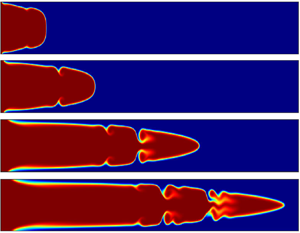
  $\textbf {B}$, the interface temporally evolves in a stable form. It shows that the product is first formed at the miscible interface between the reactants, and then diffuses with time without distorting the pure dispersive parabolic profile (see supplementary movie 1 available at https://doi.org/10.1017/jfm.2021.630). It is seen that when the flow starts inside the channel, the velocity field suddenly changes the product concentration distribution in the interior of the cell, while the product concentration at the wall changes due to diffusion only, similar to the observed phenomena between the two miscible fluid cases studied by Goyal & Meiburg (Reference Goyal and Meiburg2006). In figure 4(b), we show the corresponding time evolution of the concentration field of reactant
  $\textbf {A}$. However, if the reaction generates a more-viscous product than the reactants (i.e for
  $R_{c}=5$), we observe the formation of K–H rolling type instability in figure 4(c) (corresponding evolution of reactant
  $\textbf {A}$ is shown in figure 4d). So the question arises, how does a chemical reaction induce such instability in the flow? To understand the mechanism of the instability, we investigate the spatio-temporal evolution of a transversely averaged viscosity profile
  $\bar {\mu }_y(x,t)=\int _0^{L_{y}} \mu (x,y,t)\, \textrm {d} y$ in figure 5. The observed non-monotonic viscosity profiles at different times in figure 5 are mainly responsible for the instability. Such non-monotonic profiles are seen due to the formation of the higher viscosity product than the reactants (see the density plots of product concentration
  $c$ in figure 4c). At the
  $\textbf {A}$–
 $\textbf {C}$ interface, in the flow direction, a local increase in viscosity occurs (i.e. the viscosity gradient is from less to high), and for a favourable velocity gradient (at some positions away from both the wall and the channel centreline), such billows of K–H-type develop due to the coupling effect of shear and oscillations in the viscosity profile. Whereas at the
  $\textbf {C}$–
 $\textbf {B}$ interface, the viscosity gradient is from high to less, which opposes the growth of such roll-ups.

Figure 4. Spatio-temporal evolution of concentration of the product  $\textbf {C}$ at successive times for (a)
  $R_{c}=0$, (b) corresponding concentration evolution of reactant
  $\textbf {A}$, (c)
  $R_{c}=5$, (d) corresponding concentration evolution of reactant
  $\textbf {A}$. The other parameter values are
  $Da=50$,
  $Re=500$,
  $Pe=10\,000$.

Figure 5. Evolution of transversely averaged viscosity profile  $\bar {\mu }_{y}(x)$ in a space–time domain with
  $R_{c}=5$,
  $Da=50$,
  $Re=500$,
  $Pe=10\,000$. (Inset: the positions of the K–H billows are shown in the density plots of product concentration at
  $t=28$ by comparing the corresponding local maximums of
  $\bar {\mu }_{y}(x)$.)
The initial increment near to the inlet (at the wall) and the spike near to the tip (at the channel centreline) in the averaged viscosity profiles of figure 5 do not contribute to the K–H-instability. This is because they fall either in the zone near the wall where the axial velocity is very low or in a very high-velocity zone near the centreline. The unfavourable  $y$-gradient of the axial velocity component
  $u$ hinders the occurrence of K–H billows at these positions even though there is a viscosity stratification at the fluid–fluid interface. Furthermore, before and at time
  $t=5$, there is one local maximum between the positions of the inlet and tip (see figure 5), and this maximum attains a higher value at time
  $t=10$. Again at
  $t=10$, two more local maxima with relatively small amplitude are generated. Oscillations in the neighbourhood of these local maxima further amplify at subsequent times. These local maxima give the exact locations for where the corresponding K–H-type billows occur in figure 4(c) at the respective times. Such spatial positions of K–H-type billows in the corresponding density plot at
  $t=28$ are compared with the spatial positions of local maxima of
  $\bar {\mu }_y$ in figure 5. Hence it is evident that viscosity jumps with intermediate shear gradient produce velocity fluctuation, which leads to the formation of such roll-ups.
3.1. Reaction rate dynamics on the instability
To provide more insight into the moving reactive zone, we compute the reaction rate defined by Gérard & De Wit (Reference Gérard and De Wit2009) as
 \[ \mathcal{R}(x,y,t)= Da\, a(x,y,t) b(x,y,t). \]
Figure 6 depicts the comparison of the spatio-temporal evolution of reaction rate  $\mathcal {R}(x,y,t)$ with the product concentration
  $c$ by superimposing a representative concentration contour of
  $c=0.05$ on the density plot of
  $\mathcal {R}(x,y,t)$ for
  $R_c=5$ with
  $Da=50$,
  $Re=500$,
  $Pe=10\,000$. Interestingly, the reaction rate distribution remains very localized near the interface, despite the billows of product
  $\textbf {C}$ (see contours in figure 6) spiralling more towards the centreline of the channel due to the interplay of convection, diffusion and reaction. It is apparent from the spatial distribution of the reaction rate that, in the region where more product is formed,
  $\mathcal {R}(x,y,t)$ is decreased, which reveals the fact that a higher product concentration
  $c$ can act as a barrier for the reaction to happen. Moreover, it is noticed from the contour plots in figure 6, the roll-ups start colliding at the
  $\textbf {A}$–
 $\textbf {C}$ interface just right of the unstable billow of K–H-type and the product
  $\textbf {C}$ traps the reactant
  $\textbf {A}$ (clearly visible in the supplementary movie 3). Further, diffusion dominates, which results in the reduction of the trapped area with time, and the reaction rate
  $\mathcal {R}$ becomes negligible in that zone.

Figure 6. Temporal evolution of reaction rate  $\mathcal {R}$ (density plots) superimposed with a concentration contour of
  $c=0.05$ for
  $R_{c}=5$,
  $Da=50$,
  $Re=500$,
  $Pe=10\,000$.
3.2. Effects of the log-mobility ratio  $R_c$
$R_c$

To understand more about the influence of the log-mobility ratio on the instability, we plot the viscosity fields at a fixed time  $t=22$ for different
  $R_{c}$ values in figure 7(a) with the rest of the parameters the same as in figure 2. It is observed that even for
  $R_{c}=1$, the viscosity of the product is more than 1, no roll-ups occur (see the supplementary movie 2); however in the latter two cases, i.e. for
  $R_{c}=3$ and
  $5$, two roll-ups are formed, and the axial gap between them is increased with increasing log-mobility ratio. Such instability patterns are clearly visible in the density plot of the respective concentration field
  $a(x,y,t)$ of the reactant
  $\textbf {A}$ (see figure 7c). In order to see the effects of such
  $R_c$ on the formation of the roll-up, the corresponding transversely averaged viscosity profiles
  $\bar {\mu }_{y}(x)$ at time
  $t=22$ for different values of
  $R_c$ are shown in figure 7(b). It shows that for
  $R_c=1$, the spatially varying viscosity distributions reached a plateau; however for
  $R_c=3, 5$, the viscosity distributions oscillate with several local optimum values away from the inlet and the tip, which is the primary reason for the K–H instability in the flow. The increase in the amplitude of these oscillations with a rising log-mobility ratio (in figure 7b) explains the growing deformation of the interface. Note that the local optima of
  $\bar {\mu }_{y}(x)$ just right of the inlet and at the tip (near to channel centreline) attain higher values with increasing
  $R_{c}$. This is only a consequence of the fact that the presence of
  $\textbf {C}$ is slightly more across the
  $y$-axis than the neighbouring axial positions, and the average is taken over the
  $y$-domain. Hence, near the inlet and the tip, because of the Arrhenius relation between the viscosity and concentration
  $c$, the local optimum values increase with the increase in
  $R_{c}$. However, as previously discussed, the unfavourable
  $y$-gradient of the axial velocity component
  $u$ is responsible for the non-occurrence of K–H billows at these positions.

Figure 7. (a) Density plot of viscosity  $\mu (x,y,t)$, (b) corresponding transversely averaged viscosity profile
  $\bar {\mu }_{y}(x)$, (c) density plot of concentration
  $a(x,y,t)$ of the reactant
  $\textbf {A}$ for different values of
  $R_{c}$ at time
  $t=22$ with
  $Da=50$,
  $Re=500$,
  $Pe=10\,000$.
Unlike the averaged viscosity profiles seen in the case study of double-diffusive effects (Mishra et al. Reference Mishra, De Wit and Sahu2012), here as the viscosity is related to the product  $\textbf {C}$ only by an Arrhenius relation, it takes the constant value of one wherever the fluid
  $\textbf {C}$ is absent. In figure 6(b,c) of the paper by Mishra et al. (Reference Mishra, De Wit and Sahu2012), the averaged viscosity profile varies between two positive constants (because the flow is between two non-isoviscous bulk fluids), and instability is generated due to local increase of viscosity in the flow direction. While here, the local oscillations in the viscosity occur due to the high-viscosity product of the reaction. A spike/cap-like tip due to double diffusive effects (Mishra et al. Reference Mishra, De Wit and Sahu2012) or distortion of a mushroom-like tip (Sahu et al. Reference Sahu, Ding, Valluri and Matar2009a) occurs as the result of displacement between two non-isoviscous bulk fluids. However, here, since the displacement is between two reactant bulk fluids
  $\textbf {A}$ and
  $\textbf {B}$ of the same viscosity, and only a thin layer of a more-viscous product is formed at the interface, a Poiseuille-like tip propagates with time. K–H billows are seen only at the locations with a favourable velocity gradient where the less-viscous reactant
  $\textbf {A}$ is suspended on the more-viscous product
  $\textbf {C}$ or vice versa.
Since the more-viscous product  $\textbf {C}$ is responsible for the interfacial instability, it is crucial to do a quantitative analysis of the total product formation and its control on the instability. To do so, we compute
 \[ c_{tot}(t)=\int_{0}^{L_x}\int_{0}^{L_y} c(x,y,t) \, \textrm{d} y\,\textrm{d}{\kern0.07em}x, \]
and plot its temporal evolution for different  $R_{c}$ values in figure 8(a) while the other parameters are fixed. It is found that for the cases of
  $R_{c}=0$ and
  $R_{c}=1$, the
  $c_{tot}$ grows temporally in a similar fashion, while for the
  $R_{c}=3$ and
  $R_{c}=5$ cases, the curve deviates from that of the
  $R_{c}=0$ case after some time. Hence the instability helps in the formation of more product than the stable case. It is shown in the context of VF (Brau & De Wit Reference Brau and De Wit2020) that
  $c_{tot}$ grows as
  $t^{1/2}$ in advection–diffusion–reaction (ADR) system for a rectilinear geometry and linearly for the radial advection, where speed depends on the injection flow rate and the circle radius. Here since the channel aspect ratio is 1 : 40, the growing contact area for the reaction increases with time, as the reactive interface is axially spread over the whole domain as time evolves. Hence the total product
  $c$ grows proportional to
  $t^{1.5}$ (see the log–log plot in the inset of figure 8a for the stable case (
 $R_{c}=0$) which is an even faster rate as compared with the reactive VF results Brau & De Wit Reference Brau and De Wit2020). Moreover in the unstable situation (
 $R_{c}=5$), the product formation follows a
  $t^{1.55}$-type growth after time
  $t=10$.

Figure 8. (a) Time evolution of  $c_{tot}$ and (b) total reaction rate
  $\mathcal {R}_{tot}$ for different values of
  $R_{c}$, when
  $Re=500$,
  $Pe=10\,000$,
  $Da=50$.
To further explore the influence of instability on reaction rate with different  $R_c$, we compute
  $\mathcal {R}_{tot}(t)$ which is defined as (Gérard & De Wit Reference Gérard and De Wit2009)
 \[ \mathcal{R}_{tot}(t)=\int_{0}^{L_x}\int_{0}^{L_y} \mathcal{R}(x,y,t)\, {\textrm{d} y} \,{\textrm{d}{\kern0.07em}x}. \]
The temporal evolution of  $\mathcal {R}_{tot}(t)$ is shown in figure 8(b). It is observed that initially the
  $\mathcal {R}_{tot}$ value increases from zero to a maximum value and then starts decreasing. This is because the initial reaction area is largest when reactants
  $\textbf {A}$ and
  $\textbf {B}$ come into contact for the first time, and it subsequently decreases as the product
  $\textbf {C}$ is formed, which acts as an obstacle between the reactants to react. For the
  $R_c=0$ case (see figure 7b of Gérard & De Wit Reference Gérard and De Wit2009) in Hele–Shaw flow, i.e. for a pure reaction–diffusion (RD) systems, the total reaction rate initially attains a higher value and decreases further when the system enters diffusion-limited dynamics. However, when
  $R_c=0$ in the present channel flow case,
  $R_{tot}$ starts increasing after attaining a local minimum, unlike the Hele–Shaw flow case. The parabolic interface created from a non-uniform velocity distribution is responsible for the increasing
  $\mathcal {R}_{tot}$ for all values of
  $R_{c}$ helping the fresh reactants to come more and more into contact at successive times. Also, in contrast to the results in Hele–Shaw flow (Gérard & De Wit Reference Gérard and De Wit2009) when
  $R_c>0$, here we see that instability does not produce oscillations in the later evolution of
  $\mathcal {R}_{tot}$ after achieving the local minima. It implies that even if the interface changes its shape due to the occurrence of K–H-type billows, enough area of accessibility between the reactants
  $\textbf {A}$ and
  $\textbf {B}$ is neither frequently created nor annihilated to generate oscillations in
  $\mathcal {R}_{tot}(t)$.
3.2.1. Vorticity and enstrophy dynamics
An explanation for the mechanism of the development of roll-ups can be provided through the vorticity  $\boldsymbol {\nabla } \times V$, where
  $V=(u,v)$. To do so, we plot the vorticity field's density for different values of
  $R_{c}$ in figure 9. In the inset of figure 9, we show the vorticity's directional field at the inlet by zooming-in on the portion where the interaction of the reactant and product occurs near the wall. It is evident that when the product's viscosity increases, it acts as an obstruction to the reacting fluid that changes the direction of the flow, which can be seen from the increased bending of the directional field's arrows for a larger
  $R_{c}$ value (see figure 9). It can be seen that a horseshoe-type vortex is developing near the wall, but it cannot complete the full rotation as in the case study by Launay et al. (Reference Launay, Mignot, Riviere and Perkins2017) where the vortex is created by the interaction of a free-surface flow and an emerging obstacle. The reason is only a thin layer of high-viscosity product is acting as an obstruction to the low-viscosity reactant that affects the velocity field. The strength of the vorticity is known as the enstrophy (Miura Reference Miura1997), and can be used to understand the impact of the roll-ups on the flow globally in the whole of the channel. The enstrophy is defined as
 \[ E=\int_{0}^{L_{x}} \int_{0}^{L_{y}} (\boldsymbol{\nabla} \times V)^{2} \,{\textrm{d} y}\, {\textrm{d}{\kern0.07em}x}. \]
Indeed, Matsumoto & Hoshino (Reference Matsumoto and Hoshino2004) used its temporal evolution to find the onset of the secondary roll-ups occurring in the magnetohydrodynamic K–H instability. Hence we plot the normalized enstrophy  $E/E^{*}$ for the
  $R_{c}=3$ and
  $R_{c}=5$ cases in figure 10, where
  $E^{*}$ represents the enstrophy for the stable
  $R_{c}=0$ case. It is found that enstrophy increases monotonically with time, which reveals that roll-ups become stronger as time progresses. Also, it attains a higher value for a larger
  $R_{c}$ at each instance of time, which results in a stronger change in the directional field with increasing mobility ratio due to the presence of roll-ups with relatively higher amplitude.

Figure 9. Density plot of vorticity for different values of  $R_{c}$ at time
  $t=22$ with
  $Da=50$,
  $Re=500$,
  $Pe=10\,000$. Inset: the directional field of velocity at the inlet near the wall, where the reactant
  $\textbf {A}$ pushes the product
  $\textbf {C}$.

Figure 10. Time evolution of normalized enstrophy  $E/E^{*}$ for different values of
  $R_{c}$, when
  $Re=500$,
  $Pe=10\,000$,
  $Da=50$.
3.2.2. Mixing dynamics due to the reaction
Since the product from the reaction induces instability, we use the product concentration  $c$ to define the degree of product mixing with respect to the stable case without any loss of generality. We define the degree of product mixing as
 \[ \chi_{c}(t)=\sigma^{2}(t)/\sigma^{2}_{*}(t)-1, \]
where  $\sigma ^{2}_{*}(t)=\sigma ^{2}(t)|_{R_{c}=0}$. The global variance is known as
  $\sigma ^{2} =\langle c^{2}\rangle -\langle c\rangle ^{2}$, with
  $\langle \cdot \rangle$ denoting spatial averaging over the domain of the channel (Jha, Cueto-Felgueroso & Juanes Reference Jha, Cueto-Felgueroso and Juanes2011). Here the degree of product mixing
  $\chi _{c}(t)$ for the stable
  $R_{c}=0$ case is zero. It should be noted that here we do not have a direct relationship between
  $\sigma ^{2}$ and the dissipation rate
  $\epsilon =\langle |\boldsymbol {\nabla } c|^{2}\rangle /Pe$ (see equation (2) of Jha et al. Reference Jha, Cueto-Felgueroso and Juanes2011), as we have an entry flow situation with the reaction acting as a source term. Still, we can talk about relative mixing through
  $\chi _{c}(t)$ as a function of governing flow parameters. Figure 11(a) shows the temporal evolution of global variance
  $\sigma ^{2}$ for different values of
  $R_{c}$ with
  $Da=50$,
  $Pe=10\,000$,
  $Re=500$. The
  $\sigma ^{2}$ increases with respect to time, as the fresh product keeps forming due to reaction between
  $\textbf {A}$ and
  $\textbf {B}$. As
  $R_{c}$ increases, the value of
  $\sigma ^{2}$ also increases due to the increment of the total mass volume of the product. We plot
  $\chi _{c}(t)$ with respect to time in figure 11(b) for
  $R_{c}=3,5$ with the rest of the parameters fixed as in figure 11(a). The mixing due to the roll-ups can be analysed from the temporal evolution of
  $\chi _{c}(t)$ (figure 11b). For
  $R_{c}=3$, it shows that till
  $t\approx 10$,
  $\chi _{c}(t)$ monotonically increases to attain a maximum value then starts decreasing. However for
  $R_{c}=5$,
  $\chi _{c}(t)$ monotonically increases up to
  $t\approx 22$ with a greater value than that of the
  $R_{c}=3$ case at each instant of time. The maximum of
  $\chi _{c}(t)$ for the
  $R_{c}=5$ case is close to 0.04, which signifies the fact that an unstable case can result in
  $4\,\%$ more mixing than that of the stable case when
  $Da=50$,
  $Pe=10\,000$,
  $Re=500$. Both the curves in figure 11(b) depict that the relative mixing with respect to the
  $R_{c}=0$ case, i.e. the amount of spreading and mixing occurring in the stable case is less than that in the
  $R_{c}=3,5$ cases. In other words, the mixing occurs more efficiently due to the presence of roll-ups in the flow.

Figure 11. (a) Time evolution of  $\sigma ^{2}(t)$, (b) time evolution of
  $\chi _{c}(t)$ for different values of
  $R_{c}$, when
  $Re=500$,
  $Pe=10\,000$,
  $Da=50$.
3.3. Effects of $Da$

In this reactive flow system, the governing parameters, other than the mobility ratio  $R_c$, are Damköhler number
  $Da$, Péclet number
  $Pe$ and Reynolds number
  $Re$. To understand how these parameters influence the reactive interface's instability, we sequentially depict the effects of each of these parameters subsection-wise. In this sub-section, we discuss the effects of the Damköhler number on the flow, keeping the rest of the parameter values fixed as
  $R_{c}=5$,
  $Re=500$,
  $Pe=10\,000$. In figure 12(a) the density fields of the reactant
  $\textbf {A}$ at a fixed time
  $t=25$ are shown for different
  $Da$ values. An increase in
  $Da$ produces more product
  $\textbf {C}$ due to more consumption of reactants
  $\textbf {A}$ and
  $\textbf {B}$ in the process of the reaction. Since the product is more viscous, more formation of
  $\textbf {C}$ produces more gradient in the viscosity, which leads to high-velocity fluctuations and hence the greater deformation in the interface (see figure 12a). The reason for the formation of one billow of K–H-type, in the case of
  $Da=1$, is clear from the corresponding averaged
  $\bar {\mu }_{y}(x)$ shown in figure 12(b), as only one cycle of oscillation is present between the tip and the inlet. Similarly, for the later cases (
 $Da=10$,
  $Da=50$), more than one local optimum is seen (see figure 12b), which is depicted by the higher number of roll-ups in the density plots of figure 12(a).

Figure 12. (a) Spatial distribution of reactant  $\textbf {A}$ concentration, (b) corresponding averaged viscosity
  $\bar {\mu }_{y}(x)$ for
  $R_{c}=5$ at time
  $t=25$ for different values of
  $Da$, when
  $Re=500$,
  $Pe=10\,000$.
In figure 13(a), we plot  $c_{tot}$ against time for different values of
  $Da$. At each time with increasing
  $Da$,
$Da$,  $c_{tot}$ attains a higher value since more consumption of reactants
  $\textbf {A}$ and
  $\textbf {B}$ is enhancing the product
  $\textbf {C}$ formation. Moreover, for a smaller value of
  $Da$, although the value of
  $c_{tot}$ remains smaller as compared with the cases where
  $Da$ are large, it grows with a faster rate at a later time (
 $t>8$) than that in the case of a larger
  $Da$. This can be seen from the inset of the figure 13(a), where the log–log plot shows that, as Da increases,
  $c_{tot}$ follows
  $t^{\beta }$-type growth, where the exponent
  $\beta$ decreases from 1.93 (
 $Da=1$) to 1.55 (
 $Da=50$). However, with increasing
  $Da$, the proportionally constant (not shown) in the obtained power-law increases, so
  $c_{tot}$ attains a higher value for a higher
  $Da$ (figure 13a). As
  $Da$ is directly proportional to the reaction rate
  $\mathcal {R}(x,y,t)$,
  $\mathcal {R}_{tot}(t)$ attains a higher value for higher
  $Da$ at each instant of time (figure 13b). As mentioned earlier in § 3.2, initially
  $\mathcal {R}_{tot}(t)$ attains a higher value due to the reactive area being highest when
  $\textbf {A}$ and
  $\textbf {B}$ meet for the first time. The value of this local maximum decreases as the reaction rate slows with lower
  $Da$. When
  $Da=1$,
  $\mathcal {R}_{tot}(t)$ follows a monotonic profile since the rate of reaction is not fast enough, although the reactants
  $\textbf {A}$ and
  $\textbf {B}$ have the highest accessibility to each other at the initial stage. When the
  $Da$ value is high enough, it is evident that (see figure 13b) even though both the parabolic interface and instability accelerate the process of the reaction later, the initial reaction rate can be more than that at intermediate times.

Figure 13. (a) Time evolution of  $c_{tot}$ and (b) total reaction rate
  $\mathcal {R}_{tot}$ for different values of
  $Da$, when
  $R_{c}=5$,
  $Re=500$,
  $Pe=10\,000$.
The strengthening of the roll-ups for higher values of  $Da$ is depicted from the plots of
  $E/E^{*}$ versus
  $t$ in figure 14(a). In the case of
  $Da=1$, since there is one visible roll-up (see figure 12a) with a small amplitude, the
  $E/E^{*}$ value monotonically increases from 1 as time advances. This increment of
  $E/E^{*}$ from 1 indicates the change in the directional field from the stable situation. Other than the
  $Da=1$ case, for other three values of
  $Da$,
$Da$,  $E/E^{*}$ evolves by closely following a monotonic profile with the attainment of a higher value for a greater
  $Da$ at each time
  $t>0$. From figures 12 and 14(a), it is intuitive that in the regime of
  $Da=5$ to
  $Da=50$, the formation of only two more prominent roll-ups occurs. Moreover, adjacent smaller roll-ups to these prominent ones contribute only to a slight increment in the magnitude of the directional field compared with their corresponding stable cases. In figure 14(b) the time evolution of
  $\chi _{c}(t)$ shows when
  $Da$ is increased, more mixing occurs as compared with the stable (
 $R_{c}=0$) case. The
  $Da=1$ case is mixed less than the rest of the
  $Da$ values (
 $Da=5, 10, 50$). In the
  $Da=5$ case, the
  $\chi _{c}(t)$ profile shows monotonic increment as time advances, with a point of inflection followed by a local maximum which signifies the more nonlinear effects of K–H billows on mixing dynamics in the flow as compared with the
  $Da=1$ case. When the
  $Da$ value is further increased, the degree of mixing attains higher values than the
  $Da=5$ case at each instant of time, which indicates that more efficient mixing occurs due to stronger K–H roll-ups.

Figure 14. (a) Time evolution of scaled enstrophy  $E/E^{*}$ and (b)
  $\chi _{c}(t)$ for different values of
  $Da$, when
  $R_{c}=5$,
  $Re=500$,
  $Pe=10\,000$.
3.4. Effects of $Pe$

It should be noted here that the Péclet number  $Pe$ can be represented as the product of the Schmidt number
  $Sc$ and Reynolds number
  $Re$, i.e.
  $Pe=Re\cdot Sc$, which represents the ratio of viscous force and diffusive force. Since in the dimensional representation,
  $Pe={Q}/{D}$,
  $Re={\rho Q}/{\mu _{1}}$,
  $Sc={\mu _1}/{\rho D}$, so if we change only
  $Pe$ keeping
  $Re$ and
  $R_{c}$ fixed, then the change only corresponds to the change in solute diffusivity
  $D$. So a change in
  $Pe$ changes the diffusivity of the solutes, which implies the change in concentration profiles of both the reactants (
 $\textbf {A}$ and
  $\textbf {B}$) and the product
  $\textbf {C}$ at the wall (Goyal & Meiburg Reference Goyal and Meiburg2006). Thus near the impermeable rigid upper and lower walls, the reactive interface moves further right of the inlet for a lower
  $Pe$ due to more solute diffusion as compared with that of a higher
  $Pe$, which is clearly reflected in figure 15(a). When
  $Pe$ increases, the effectiveness of interfacial roll-ups on the interface deformation reduces (see figure 15a). The diffusion zone decreases in reactants with an increase of
  $Pe$, which reduces the area where the product concentration is non-zero. Hence the viscosity at each axial station attains a higher value with a decrease in
  $Pe$ (see figure 15b), which implicitly helps to produce more favourable conditions to have oscillations in the viscosity profile. The interface deforms more when
  $Pe=5000$ than the case where
  $Pe=50\,000$. It is essential to note that, in experiments, the change in
  $Pe$ is often done by tuning the dimensional flow rate
  $Q$, so we briefly explained how the change in the flow rate
  $Q$ affects the presented system in Appendix A.

Figure 15. (a) Spatial distribution of reactant  $\textbf {A}$ concentration and (b) corresponding averaged viscosity
  $\bar {\mu }_{y}(x)$, for
  $R_{c}=5$ at time
  $t=25$ for different values of
  $Pe$, when
  $Re=500$,
  $Da=50$.
It can be observed from figure 16(a),  $c_{tot}$ increases monotonically with respect to time for different values of
  $Pe$, when the rest of the governing parameters are fixed. However, since
  $Pe$ is inversely proportional to the diffusivity of solutes, a lower
  $Pe$ results in more product
  $\textbf {C}$ formation and hence a greater value of
  $c_{tot}$. When
  $Pe$ increases, the concentration layer of the product
  $\textbf {C}$ between
  $\textbf {A}$ and
  $\textbf {B}$ gets thinner due to less diffusivity, which favours more access of
  $\textbf {A}$ to
  $\textbf {B}$ (Gérard & De Wit Reference Gérard and De Wit2009) and vice versa. Hence
  $\mathcal {R}_{tot}(t)$ attains a higher value for each time for a greater
  $Pe$ (figure 16b). This phenomenon can be easily verified from the colour bars of the density plot of the reaction rate for different values of
  $Pe$ in figure 17, which reveals the higher values of the reaction rate for a greater
  $Pe$. Again, the initially attained maximum value of
  $\mathcal {R}_{tot}(t)$ also becomes lower with a lower
  $Pe$ value because the domination of convection over diffusion helps
  $\textbf {A}$ and
  $\textbf {B}$ to react more (figure 16b). Hence from figures 16 and 17, it is clear that a lower value of
  $Pe$ helps to produce more
  $\textbf {C}$ (value of
  $c_{tot}$ is larger), which makes
  $\textbf {A}$ and
  $\textbf {B}$ less accessible to each other as the product
  $\textbf {C}$ is formed between them, thus
  $\mathcal {R}_{tot}(t)$ is smaller.

Figure 16. (a) Time evolution of  $c_{tot}$ and (b) total reaction rate
  $\mathcal {R}_{tot}$ for different values of
  $Pe$, when
  $R_{c}=5$,
  $Re=500$,
  $Da=50$.

Figure 17. Spatial distribution of reaction rate at  $t=25$ for different values of
  $Pe$, when
  $R_{c}=5$,
  $Re=500$,
  $Da=50$.
As discussed previously, since the  $Pe$ is inversely proportional to the diffusivity of solute concentrations, a lower
  $Pe$ results in more production of fluid
  $\textbf {C}$, which implicitly causes the formation of the roll-ups with a relatively high amplitude compared with that for a higher
  $Pe$ value. Therefore, the integral of the square vorticity over the channel attains a higher value with a lower
  $Pe$. This can be observed from the scaled temporal evolution of enstrophy for different
  $Pe$ values shown in figure 18(a). It is found that the degree of product mixing,
  $\chi _{c}(t)$, is less in the case of a lower
  $Pe$ than that with a higher
  $Pe$ value at each instant of time (figure 18b). This result is counter-intuitive, because the interface is more deformed for a lower value of
  $Pe$ (see figure 15). However, here we are measuring the degree of product mixing with respect to the corresponding stable
  $R_{c}=0$ case. Moreover, for a lower
  $Pe$ value, the interface of the stable situation is relatively more diffusive. So even if there are K–H billows for the unstable
  $R_{c}=5$ case, a lower
  $Pe$ case produces less effective mixing than its corresponding stable case.

Figure 18. (a) Time evolution of scaled enstrophy  $E/E^{*}$ and (b)
  $\chi _{c}(t)$ for different values of
  $Pe$, when
  $R_{c}=5$,
  $Re=500$,
  $Da=50$.
3.5. Effects of $Re$

When only the Reynolds number  $Re$ is increased and the rest of the parameters are kept fixed, we observed that the biggest K–H billow is stronger and develops rapidly at the reactive
  $\textbf {A}$–
 $\textbf {C}$ front (see figure 19a). Again for different
  $Re$, the solute diffusion that occurs near the wall remains constant (since the
  $Pe$ is kept constant), so the interface pattern near the channel entrance remains the same. It is also observed that reduction of velocity at the tip front and transverse-widening of the reactive front occurs at the tip with increasing
  $Re$. Hence, for a lower inertia flow i.e
  $Re=250$, enough velocity fluctuations leading to roll-ups are not achieved as compared with
  $Re=500, 1000$. The transverse widening phenomenon decreases the angle of inclination of the interface from the wall to the front-tip, which reduces invasion of the product
  $\textbf {C}$ into
  $\textbf {A}$. So the first noticeable roll-up (right of the inlet) is smaller in the case of
  $Re=1000$ than
  $Re=500$. However, the deformation near the biggest roll-up left of the tip increases with increasing
  $Re$, as the inclination is more favourable for the instability at those axial positions. These effects can be clearly seen through the amplitude of oscillations in the transversely averaged viscosity profile
  $\bar {\mu }_{y}(x)$ (see figure 19b).

Figure 19. (a) Spatial distribution of reactant  $\textbf {A}$ concentration and (b) corresponding averaged viscosity
  $\bar {\mu }_{y}(x)$, for
  $R_{c}=5$ at time
  $t=25$ for different values of
  $Re$, when
  $Pe=10\,000$,
  $Da=50$.
As observed from figure 19, the reduction of the velocity at the front-tip occurs with increasing  $Re$, so with a greater
  $Re$ value, the product spreads less in the axial direction of the flow in the channel. Again, for the
  $Re=500$ case (figure 19) the number of larger roll-ups is more as compared with the
  $Re=2000$ case, even though the
  $Re=2000$ case has more roll-ups of small amplitude in the axial positions between
  $x=10$ and
  $x=15$. Thus due to the following two facts, (1) the axial spreading of the product
  $\textbf {C}$ is more and (2) more invasion of product
  $\textbf {C}$ due to favourable angle of inclination results in a higher number of bigger roll-ups,
  $c_{tot}$ becomes smaller with the increase of
  $Re$ (figure 20a). Moreover, the later time evolution of
  $c_{tot}$ reveals that the two cases of
  $Re=500, 1000$ grow closely as do the cases of
  $Re=2000$, 2500. In figure 20(b), we show the temporal evolution of
  $\mathcal {R}_{tot}(t)$ while keeping rest of the parameters fixed as
  $R_{c}=5$,
  $Pe=10\,000$,
  $Da=50$. Since the solute diffusion is the same (constant
  $Pe$) the thickness of the reactive interface is the same, so it is only due to the coupling effect of convection and viscous dissipation that a higher number of bigger K–H-billows produce more favourable conditions for the accessibility of
  $\textbf {A}$ and
  $\textbf {B}$ to react. So the value of
  $\mathcal {R}_{tot}(t)$ becomes lower when
  $Re$ is increased from 500 to 2500.

Figure 20. (a) Time evolution of  $c_{tot}$ and (b) total reaction rate
  $\mathcal {R}_{tot}$ for different values of
  $Re$, when
  $R_{c}=5$,
  $Pe=10\,000$,
  $Da=50$.
The number of comparably bigger roll-ups decreases with the increase of  $Re$ from
  $500$ to
  $2000$ (figure 19), hence the strength of vorticity. This is reflected from the plots of
  $E/E^{*}$ in figure 21(a). Moreover it is observed (not shown) that after time
  $t \ge 15$,
  $E/E^{*}$ follows a linear-type growth for each value of
  $Re$. Again, as previously noticed in figure 20, a similar closeness of two pairs (
 $Re=500$, 1000 and
  $Re=2000$, 2500) of Reynolds numbers occurs in the evolution of
  $E/E^{*}$. The degree of product mixing also attains a higher value for a lower
  $Re$ (figure 21b). Moreover,
  $\chi _{c}(t)$ is positive and monotonically increases with increasing time up to
  $t \lesssim 22$ for
  $Re=500$, and when
  $t > 22$ it starts to decrease to a local minimum (at
  $t\approx 27$) and then again increases. These nonlinear-type evolutions of
  $\chi _{c}(t)$ can be thought as a consequence of the coupling effects of CDR at later times (see supplementary movie 3). For
  $Re=1000$,
  $\chi _{c}(t)$ increases up to
  $t \approx 8$ then slightly decreases to attain a local minimum at
  $t \approx 14$ and then again increases but with a lower value at each time
  $t$ for
  $(0, 26.5)$ than that of the
  $Re=500$ case. At
  $t\approx 26.5$,
  $\chi _{c}(t)$ becomes equal for both
  $Re=500$ and
  $Re=1000$, and then for
  $Re=1000$ it becomes larger revealing that after a certain time mixing can be more efficient than that in the case of
  $Re=500$. When
  $Re$ is further increased to
  $Re=2000$, it is seen that
  $\chi _{c}(t)$ increases initially up to a time
  $t \approx 6.5$, then it starts decreasing to attain a negative local minimum at
  $t \approx 15$ and monotonically increases at later times (see figure 21b). Again for
  $Re=2500$ it is noticed that the degree of mixing is positive initially for a smaller interval than the case when
  $Re=2000$, and
  $\chi _{c}(t)$ becomes negative after
  $t\gtrsim 9$, which implies that when the number of roll-ups decreases significantly, the stable case can become more efficient in mixing than an unstable case.

Figure 21. (a) Time evolution of scaled enstrophy  $E/E^{*}$ and (b)
  $\chi _{c}(t)$ for different values of
  $Re$, when
  $R_{c}=5$,
  $Pe=10\,000$,
  $Da=50$.
To understand why  $\chi _{c}(t)$ increases to reach a maximum value (in the case of
  $Re=2000$) then starts decreasing to a local minimum, then again increases, we compare the time evolution of the rate of change in variance
  $\textrm {d} \sigma ^{2}(t)/\textrm {d}t$ (Jha et al. Reference Jha, Cueto-Felgueroso and Juanes2011) for
  $R_{c}=0$ and five cases with fixed
  $Re=2000$ in figure 22(a,b). It is clear that
  $\textrm {d} \sigma ^{2}(t)/\textrm {d}t$ for the stable case (
 $R_{c}=0$) becomes larger and exceeds that of the corresponding unstable case (
 $R_{c}=5$) at a time
  $t \approx 6.5$. Further the rate of change in variance
  $\textrm {d} \sigma ^{2}(t)/\textrm {d}t$ for
  $R_{c}=0$ gets lower than that of the
  $R_{c}=5$ case at a later time
  $t \approx 15$. The local maximum and minimum observed in the curve of
  $\chi _{c}(t)$ in figure 21(b) (for
  $Re=2000$), correspond to these cross-over times (i.e. at
  $t \approx 6.5$ and 15, respectively) for the rate of change of variance between the
  $R_{c}=0$ and
  $R_{c}=5$ cases. This happens because the
  $R_{c}=0$ case is an ADR system and there is a time zone for which the diffusive interface of the stable
  $R_{c}=0$ helps to provide a faster monotonic increment of
  $\sigma ^{2}(t)$ giving rise to such oscillatory phenomena in
  $\chi _{c}(t)$.

Figure 22. (a) The rate of change in variance  ${\textrm {d}\sigma ^{2}}/{\textrm {d}t}$ becomes greater after
  $t \gtrsim 6.51$ for the
  $R_{c}=0$ case than that for the
  $R_{c}=5$ case, (b)
  ${\textrm {d}\sigma ^{2}}/{\textrm {d}t}$ again becomes smaller at a later time
  $t \gtrsim 14.9$ for the
  $R_{c}=0$ case than that for the
  $R_{c}=5$ case when
  $Re=2000$,
  $Pe=10\,000$,
  $Da=50$. (c) Time evolution of
  $\chi _{c}(t)$ for different values of
  $Pe$, when
  $Re=2000$,
  $R_{c}=5$,
  $Da=50$.
Interestingly, it is observed that if the number of roll-ups is significantly less (which happens for  $Re=2000, 2500$), the degree of mixing can become even negative (see figure 21b); this signifies the variance of the
  $R_{c}=0$ case is more than that of the
  $R_{c} =5$ case, for large
  $Re = 2000$ and 2500, within a certain time interval. It is noteworthy that the degree of mixing reported by Jha et al. (Reference Jha, Cueto-Felgueroso and Juanes2011) only takes positive values because it is relatively defined with respect to the initial segregated state for which there is no advection and diffusion. However, here,
  $\chi _{c}(t)$ is relatively defined with respect to the stable
  $R_{c}=0$ case, which itself is an ADR system, so the negativity of
  $\chi _{c}(t)$ is justified. Moreover, in the ADR system of the
  $R_{c}=0$ case, the thickness of the reactive interface (the mixing zone) depends on solute diffusivity, and again from subsection 3.4, it is seen that when
  $Pe$ increases, the degree of product mixing increases (see figure 18b). So it would be beneficial to check the effects of solute diffusion for the
  $Re=2000$ case, which may answer why at a certain time interval the stable
  $R_{c}=0$ case produces more efficient mixing than the unstable
  $R_{c}=5$ case. Thus in figure 22(c) we show the evolution of
  $\chi _{c}(t)$ for
  $Re=2000$ by comparison with the cases where solute diffusion is relatively more dominated by convection (for larger Péclet values). The plots from figure 22(c) reveal that
  $\chi _{c}(t)$ is positive for both
  $Pe=25\,000$, 25 000, implying, even though there are roll-ups in the unstable
  $R_{c}=5$ case,
  $R_{c}=0$ can produce efficient mixing at certain times only when the thickness of the mixing layer is greater due to more solute diffusion. Also it can be implicated that, for each
  $Pe$ value in figure 22(c),
  $\chi _{c}(t)$ decreases in the diffusion-dominated time regime of the corresponding
  $R_{c}=0$ case. Moreover, after attaining the local minimum,
  $\chi _{c}(t)$ again increases since the contribution of K–H roll-ups to the mixing amplifies as several roll-ups break-up and diffusive plume creation occurs due to the effects of the nonlinear phenomenon. In this time regime, since the interface is more distorted for a lower
  $Pe$ (for example check figure 15a),
  $\chi _{c}(t)$ can take a higher value for lower
  $Pe$ (see figure 22c).
3.6. Onset of instability
In order to understand the early stages of complex interfacial patterns formed due to the coupling of CDR dynamics in this flow system, we evaluate the onset of instability from the present nonlinear simulations. The onset time is defined as
 \[ t_{on}=\min_{t\ge 0}(\lvert I(t) - I^{*}(t) \rvert > \tau), \]
where  $I(t)$ is the interfacial length computed as (Sharma et al. Reference Sharma, Pramanik, Chen and Mishra2019)
 \[ I(t)=\int_{0}^{L_x}\int_{0}^{L_y} \sqrt{\left(\frac{\partial a}{\partial x}\right)^{2}+ \left(\frac{\partial a}{\partial y}\right)^{2}} {\textrm{d} y} \,{\textrm{d}{\kern0.07em}x}, \]
and  $I^{*}(t)=I(t)|_{R_c=0}$. The threshold value
  $\tau =\max (| I(t) - I^{*}(t)| :t \ge 0))$ for
  $R_{c}=1$ as it represents a stable situation (figure 4a,b).
It is noticed (not shown) that  $I(t)$ increases slightly for
  $R_{c}=1$ than that for
  $R_{c}=0$, but in this case, enough viscosity contrast (figure 7a,b) is not generated for the K–H instability. Hence a small value of threshold
  $\tau$ is required in the definition of
  $t_{on}$ to capture the correct onset time, and it can be thought of as a minimum value that can be ignored to distinguish an unstable system from a stable one. The exact value of
  $\tau$ considered here is given below.
In figure 23 we plot the calculated onset time  $t_{on}$ against
  $R_c$ for different values of
  $Da$ fixing
  $Re=500$,
  $Pe=10\,000$. It is observed that for a fixed
  $R_{c}$ value with increasing
  $Da$, instability triggers early, this is because of the fast rising viscosity gradient near the interface as product formation process is enhanced by higher
  $Da$ values. The process of rising viscosity gradient is also fastened with increasing
  $R_{c}$, hence for a fixed
  $Da$,
$Da$,  $t_{on}$ decreases with increasing
  $R_{c}$ (figure 23). The (
 $t_{on}$–
 $R_{c}$) space partitions into stable and unstable time zones for each value of
  $Da$, which is clearly indicated through corresponding interfacial patterns of the product concentration field in the respective zones (in the insets of figure 23). For example, the patterns at the onset time
  $t_{on} \approx 13.8$ for
  $Da =50$,
  $R_{c}=2$ indicate the appearance of the instability. Here, the value of the threshold
  $\tau$ is considered to be
  $0.3$, which is found to be
  ${\approx }0.9\,\%$ of
  $I^{*}(t_{on})$.

Figure 23. Onset of the instability  $t_{on}$ versus
  $R_{c}$ for different
  $Da$ when
  $Re=500$,
  $Pe=10\,000$. Inset: product concentration field in the lower half of the channel indicating the patterns at the stable and unstable zones.
The onset of instability as a function of both  $R_{c}$ and
  $Pe$ is depicted in figure 24, which shows the
  $t_{on}$ decreases when
  $R_c$ increases and if
  $Pe$ increases then
  $t_{on}$ increases. So when
  $R_{c}$ tends to zero the onset time tends to infinity and for a higher Péclet value the unstable zone becomes smaller. The graphs from figure 24 show that when
  $Pe$ is increased, i.e. the solute diffusion is decreasing, its effect on the flow not only results in the suppression of K–H-instability but also delays the instability to occur. By observing the trends in these curves for different
  $Pe$, interestingly we could normalize the
  $t_{on}$ by a factor
  $(\alpha \cdot Pe + \beta )$, with
  $\alpha =0.1$ and
  $\beta =10$, so that the rescaled onset time
  $t_{on}^{*}$ versus
  $R_c$ clearly depicts the independence of
  $Pe$ i.e. the solute diffusion effects can be rescaled to divide the
  $(t^{*}_{on}, R_{c})$ space into stable and unstable time zones with a single partitioning curve.

Figure 24. Onset of the instability  $t_{on}$ versus
  $R_{c}$ for different
  $Pe$ when
  $Da=50$,
  $Re=500$. Inset: re-scaled
  $t_{on}^{*}(= t_{on}/(\alpha \cdot Pe + \beta ))$ versus
  $R_c$ shows the proportionate dynamics of
  $Pe$, where
  $\alpha =0.1$ and
  $\beta =10$.
The plots of onset of the instability  $t_{on}$ as a function of different
  $R_{c}$ and
  $Re$ (with fixed
  $Da$ and
  $Pe$) are shown in figure 25(a). Interestingly it is found that if
  $R_{c} \ge 2.5$, then the onset of instability is earlier when the
  $Re$ value is increased from 500 to 2500. This is very counter-intuitive as the number of bigger roll-ups decreases with increasing
  $Re$ from 500 to 2000 (figure 19) when
  $R_{c}=5$. Also
  $c_{tot}$ and
  $\mathcal {R}_{tot}$ decrease with increasing
  $Re$ (figure 20a,b), which reveals that instability neither enhances the production process of
  $\textbf {C}$ nor creates favourable conditions for the accessibility of reactants
  $\textbf {A}$ and
  $\textbf {B}$ for a larger
  $Re$. Thus it can be implicated from figure 19, the biggest K–H billow just before the tip of the reactive front starts forming early when
  $Re$ is increased, and this not only happens for
  $R_{c}=5$, but also for all the values of
  $R_{c}$ in the interval
  $[2.5, 7]$. To verify the claim that the development of the biggest roll-up near the tip contributes to early onset for a larger
  $Re$, when
  $R_{c} \ge 2.5$, we show the zoomed-in density plots of the product
  $\textbf {C}$ in the upper half of the channel (since the flow feature is symmetric around the middle of the channel) for different
  $Re$ values at time
  $t=8$ in figure 25(b). Note that
  $t=8$ is the onset time for
  $R_{c}=3$,
  $Re=1000$ and at this time the growth of the biggest roll-up near to the tip is indicated by a white arrow. It can be easily checked at this time that the roll-up corresponding to the
  $Re=500$ case has not developed much as compared with the
  $Re=1000$ case. Hence the onset must be delayed for the case when
  $R_{c}=3$,
  $Re=500$, which is clearly depicted in figure 25(a). Again when
  $Re=2000$, 2500, onset is very close to each other and earlier than in the
  $Re=1000$ case, which is justified from the density plots, i.e. the roll-up has grown more as compared with
  $Re=1000$ at time
  $t=8$ in these two cases. We checked that the monotonic dependence of the onset on
  $Re$, i.e. when
  $Re$ decreased from a high to low value the onset becomes earlier, holds not only for
  $R_{c}=3$ but also for all
  $R_{c} \in [2.5, 7]$. It is also noticed that the amplitude of the oscillation in the averaged viscosity profile (figure 19b) corresponding to the largest roll-up for the case of
  $Re=2000$ and
  $R_{c}=5$ is decreased slightly compared with that of the
  $Re=500$,
  $R_{c}=5$ case. As shown in figure 7(b), the amplitude of oscillations decreases with the decrease in
  $R_{c}$ when the rest of the parameters are fixed. So, when
  $R_{c}< 2.5$, for the
  $Re=2000$ and
  $Re=2500$ cases, the amplitude of the largest K–H billow is reduced by such an amount that it does not form early as compared with the
  $Re=500$ and
  $Re=1000$ cases. This can be seen from the trends of
  $t_{on}$ shown in figure 25(a). Also
  $t_{on}$ attains a greater value for the case of
  $Re=2500$ than that of
  $Re=2000$ if
  $R_{c} \le 2$. To verify the above claim we show the zoomed-in density plots of the product
  $\textbf {C}$ for different
  $Re$ at time
  $t=14$ in figure 25(c). It is to be noted that
  $t=14$ is very close to the onset time for the
  $R_{c}=2, Re=500$ case. The white arrow points out the biggest roll-up near to the tip and it can be seen that this roll-up has grown more in the
  $Re=1000$ case compared with that of the
  $Re=500$ case at the same time
  $t=14$. So the onset is earlier for
  $Re=1000$ than
  $Re=500$ as depicted by figure 25(a). Again, when
  $Re$ increases to a value of 2000, this roll-up has not formed yet at the time
  $t=14$, and even for
  $Re=2500$ the development of the roll-up is comparably less than the
  $Re=2000$ case. So for
  $Re=2000$ the onset is more delayed than the cases when
  $Re=500$, 1000 and it attains an even greater value for
  $Re=2500$ (
 $t_{on} \approx 18$). Hence from figure 25, it is clear that the onset dynamics can reversely depend on lower
  $R_{c}$ values for higher values of
  $Re$.
$Re$.

Figure 25. (a) Onset of the instability  $t_{on}$ versus
  $R_{c}$ for different
  $Re$ when
  $Da=50$,
  $Pe=10\,000$. (b) Zoomed-in density plots of concentration of the product
  $\textbf {C}$ at time
  $t=8$ for different
  $Re$ when
  $R_{c}=3$,
  $Da=50$,
  $Pe=10\,000$. (c) Zoomed-in density plots of concentration of the product
  $\textbf {C}$ at time
  $t=14$ for different
  $Re$ when
  $R_{c}=2$,
  $Da=50$,
  $Pe=10\,000$.
4. Conclusion
The intent of this paper has been to investigate numerically how a chemical reaction can induce interfacial instabilities in a pressure-driven channel flow where the displacement is between two isoviscous reactants. Such instability in the form of billows of K–H-type arises from the formation of the high-viscosity product at the interface of both chemical reactants. Interestingly, a laminar horseshoe-type instability near the wall is also observed, which results from the obstruction of the less-viscous reactant by the more-viscous product at the inlet. We demonstrated the effects of the dimensionless parameters, such as the log-mobility ratio  $R_{c}$, Damköhler number
  $Da$, Péclet number
  $Pe$ and Reynolds number
  $Re$, on the instability patterns of the ‘interface’ separating the fluids. The impact of the instability on the total production of the product
  $\textbf {C}$ (
 $c_{tot}$) and total reaction rate (
 $\mathcal {R}_{tot}$) are discussed. The development of K–H roll-ups through the strength of the vorticity is analysed. The influence of the instability on the mixing is explored through
  $\chi _{c}(t)$ as a function of non-dimensional numbers that govern the flow.
It is found that the onset of the instability is early for larger  $Da$,
$Da$,  $R_{c}$ but delayed when
  $Pe$ is increased. However the onset is early for an increasing value of
  $Re$ only if
  $R_{c}\ge 2.5$ and when
  $R_{c} < 2.5$ the onset for a higher
  $Re$ may be delayed. It is also noteworthy that
  $Pe$ effects on the onset time can be linearly scaled to justify a proportionate dynamics, which defines an approximate boundary between stable and unstable time zones. Moreover, since
  $t_{on}$ (as a function of
  $Da$,
$Da$,  $Re$ and
  $Pe$) is asymptotically tending to infinity when
  $R_{c}$ tends to zero, and for some positive
  $R_{c}$ values it is unattainable before the reactant
  $\textbf {A}$ reaches the outlet of the channel, the existence of a critical
  $R_c$ is implied with a fixed
  $Da$,
$Da$,  $Re$ and
  $Pe$ for the instability to occur. The increase in
  $Re$ favours more instability at certain axial positions, where it can suppress the amplitude of the unstable billows at some other axial locations. It should be noted that the present numerical study is only an initiation towards a qualitative description of the experimental shear-flow instability induced by a chemical reaction in channel geometry reported by Burghelea et al. (Reference Burghelea, Wielage-Burchard, Frigaard, Martinez and Feng2007) and motivates further possible experimental work in this area of reaction modulated pattern formations.
Supplementary movies
Supplementary movies are available at https://doi.org/10.1017/jfm.2021.630.
Funding
M.M. acknowledges the financial support from SERB, Government of India through project grant no. CRG/2020/000613. S.N.M. also acknowledges the support of UGC, Government of India with research fellowship Ref. No. 1112/(OBC)/(CSIR-UGC NET DEC. 2016).
Declaration of interests
The authors report no conflict of interest.
Appendix A
Since the Péclet number  $Pe={Q}/{D}$, it can be varied through the flow rate
  $Q$ only while keeping the solute diffusivity (
 $D$) constant. The previous discussions (in § 3) are presented by treating the effects of the solutes diffusion (3.4) and momentum diffusion (§ 3.5) separately. So we did not vary ‘only’ the dimensional flow rate
  $Q$ anywhere, as the change in flow rate corresponds to a change in
  $Re$. So if solute diffusivity
  $D$ is fixed, then we need to write
  $Pe$ in the form of
  $Re \cdot Sc$ (Sahu et al. Reference Sahu, Ding, Valluri and Matar2009a; Mishra et al. Reference Mishra, De Wit and Sahu2012). Thus the non-dimensional system reduces to the following:
 \begin{gather} \boldsymbol{\nabla} \boldsymbol{\cdot} \boldsymbol{u} = 0, \end{gather}
 \begin{gather}\left[ \frac{\partial \boldsymbol{u}}{\partial t} +\boldsymbol{u \cdot \nabla} \boldsymbol{u} \right] ={-}\boldsymbol{\nabla} p + \frac{1}{Re}\boldsymbol{\nabla} \boldsymbol{\cdot} [\mu(c) (\boldsymbol{\nabla} \boldsymbol{u}+ \boldsymbol{\nabla} \boldsymbol{u}^{T}) ], \end{gather}
 \begin{gather}\frac{\partial a}{\partial t} +\boldsymbol{u \cdot \nabla} a = \frac{1}{Re.Sc} \nabla^{2} a-Da \, ab, \end{gather}
 \begin{gather}\frac{\partial b}{\partial t} +\boldsymbol{u \cdot \nabla} b = \frac{1}{Re.Sc} \nabla^{2} a-Da\, ab, \end{gather}
 \begin{gather}\frac{\partial c}{\partial t} +\boldsymbol{u \cdot \nabla} c = \frac{1}{Re.Sc} \nabla^{2} c+ Da\, ab, \end{gather}
 \begin{gather}\mu = \textrm{e}^{R_{c} c}. \end{gather}
Now a change in  $Re$ affects both the coefficient of viscous dissipation in (A1b) and the coefficient of solute diffusion terms in (A1c–e). This, in turn, changes both the wall effects at the inlet due to solute diffusion and transverse widening of the front tip due to a change in momentum simultaneously. This can be easily noticed from figure 26(a,b). However, in § 3.5, effects of
  $Re$ are explained by keeping
  $Pe$ fixed, i.e. the ratio
  ${Q}/{D}$ is fixed, which has the advantage that wall effects at the inlet remain the same since the impact of solute diffusion is the same (see figure 18).

Figure 26. (a) Density plots of reactant  $\textbf {A}$ at time
  $t=25$ for different values of
  $Re$, when
  $R_{c}=5$,
  $Sc=20$,
  $Da=50$. (b) Corresponding transversely averaged viscosity profiles.


