


1. Introduction
Viscoelastic fluids encompass a wide variety of physical systems that have as a common feature the ability to develop both viscous and elastic properties under the same conditions. They include different types of liquids, colloids, polymers, organic and polymer alloys and a number of biological materials. Regardless of the considered specific chemical composition, intriguing and original dynamics generally originates from the property of these fluids to retain stresses even in the absence of a gradient of velocity and the ensuing ability to produce highly nonlinear behaviour; while an initial flow can produce long-chain molecules stretching, the deformation of the molecules (evolving with a characteristic time that does not match that of the main flow) can cause secondary flows which further stretch them, thereby allowing the amplification of an initial small disturbance through an iterative cause-and-effect coupling mechanism. Remarkably, by virtue of these peculiar feedback loops, chaos can be excited in these liquids using more viscous solutions, which is a rather counterintuitive concept if it is considered in the frame of existing theories for the onset of (inertial) turbulence in conventional fluids (Larson, Shaqfeh & Muller Reference Larson, Shaqfeh and Muller1990; Larson Reference Larson1992; Groisman & Steinberg Reference Groisman and Steinberg1998, Reference Groisman and Steinberg2000; Morozov & van Saarloos Reference Morozov and van Saarloos2005; Lappa Reference Lappa and Lindholm2019a).
Related problems are generally challenging because of the importance of interactions across many length and time scales, the existence of multiples solutions, the high sensitivity to initial conditions and the often non-trivial geometry and topology of the emerging flow.
Leaving aside for a while the inherent theoretical complexities, this category of fluids is central to several technological applications in the chemical, cosmetic, pharmaceutical, materials, energy and food industries. Typical applications deal with plastics joining (Rotheiser Reference Rotheiser1999; Troughton Reference Troughton2008), heating of polymers required for mechanical and tribological properties improvement (Aly Reference Aly2015 and references therein), the welding of plastics (Grewell & Benatar Reference Grewell and Benatar2007), fibre spinning and fibre casting, film blowing and extrusion processes (Chung Reference Chung2010; Rauwendaal Reference Rauwendaal2013), coating, painting, printing (Petrie & Denn Reference Petrie and Denn1976), biological reactors, microfluidic devices and many other processes in engineering (Bonito, Clément & Picasso Reference Bonito, Clément, Picasso, Glowinski and Xu2011).
Given the above rationale, our article addresses a dilemma that continues to challenge the scientific community, namely, the evolution of certain flows of natural origin (induced by gravity) that are produced in viscoelastic fluids when they are exposed to heat. As outlined above, in the liquid phase, elastic stresses typically develop, which contribute, together with the classical stresses of viscous nature, to determine the response of these fluids to the application of thermal stimuli. Here, in particular, we consider a very classical problem, i.e. the onset of buoyancy convection in systems uniformly heated from below and cooled from above, corresponding to the so-called Rayleigh–Bénard paradigm. This type of convection is known to produce such a variegated set of different structures and bifurcations that it has been considered for a long time as a universal testbed for the study of the typical properties of dissipative systems and their related evolution (Crespo del Arco et al. Reference Crespo del Arco, Bountoux, Sani, Hardin and Extrémet1988; Crespo Del Arco & Bontoux Reference Crespo del Arco and Bontoux1989; Clever & Busse Reference Clever and Busse1993, Reference Clever and Busse1994; Gelfgat Reference Gelfgat1999; Delgado-Buscalioni, Crespo del Arco & Bontoux Reference Delgado-Buscalioni, Crespo del Arco and Bontoux2001; Xi, Lam & Xia Reference Xi, Lam and Xia2004; Sun et al. Reference Sun, Xia and Tong2005; Lappa Reference Lappa2009; Xie et al. Reference Xie, Cheng, Hu and Xia2019).
Prior to expanding on the present results, we provide the reader with a brief account of the historical perspective that produced a high level of interest in the peculiar path taken by this type of flow in viscoelastic fluids when they evolve from an initial quiescent state.
In particular, it is convenient to start to deal with such a topic by considering the pioneering theoretical analyses by Green (Reference Green1968), Vest & Arpaci (Reference Vest and Arpaci1969) and Sokolov & Tanner (Reference Sokolov and Tanner1972), where for the first time the concept of elastic overstability was introduced, i.e. that due to the competition between the processes of viscous relaxation and thermal diffusion; viscoelastic effects can produce convective modes that become unstable at a Rayleigh number that is smaller than that predicted for the corresponding stationary convection in Newtonian fluids. The first solid theoretical underpinnings for such a realization emerged naturally out of the mathematics behind the so-called linear stability analysis techniques (LSA). Due to such studies, eventually, it was recognized (see Martínez-Mardones & Pérez-Garcíıa Reference Martínez-Mardones and Pérez-Garcíıa1990; Larson Reference Larson1992) that viscoelastic forces can produce completely new mechanisms for instability that are not possible in flows of non-polymeric Newtonian fluids. A masterful exposition on the state of the art about LSA can be found in Park & Lee (Reference Park and Lee1996) and Li & Khayat (Reference Li and Khayat2005), where this dynamics has been properly categorized in terms of two distinct regions of the space of parameters, namely the weakly elastic regime (WER) and the strongly elastic regime (SER).
While WER is generally assumed to be extended from θ = 0 to θh, where θ is the so-called elasticity parameter (directly proportional to the product of the fluid thermal diffusivity and its relaxation time and inversely proportional to the square of a characteristic length, see § 2) and θh is the level of elasticity below which stationary flow occurs as the primary mode of convection, SER (where the role of primary convective mode is taken over by oscillatory flow) is attained for θ > θh. As explained above, in the latter case, the initial quiescent thermally diffusive state undergoes a Hopf bifurcation for a value of the Rayleigh number that is smaller than that required to produce steady convection in an equivalent Newtonian fluid.
The need to predict the effective patterning behaviour and the magnitude of convection amplitude in the post-critical regime led many investigators to reconsider the stability problem in the framework of weakly nonlinear analyses based, e.g. on amplitude equations, the power-series method and other similar approaches. Relevant examples along these lines are the works by Eltayeb (Reference Eltayeb1977), Rosenblat (Reference Rosenblat1986), Martínez-Mardones & Pérez-Garcíıa (Reference Martínez-Mardones and Pérez-Garcíıa1992), Martínez-Mardones et al. (Reference Martínez-Mardones, Tienmann, Walgraef and Zeller1996), Park & Lee (Reference Park and Lee1996), Parmentier, Lebon & Regnier (Reference Parmentier, Lebon and Regnier2000) and Li & Khayat (Reference Li and Khayat2005). Relying on this approach, interestingly, Martínez-Mardones et al. (Reference Martínez-Mardones, Tienmann, Walgraef and Zeller1996) determined the stability range for standing waves potentially emerging in the SER in proximity to the instability threshold. Vice versa, Parmentier et al. (Reference Parmentier, Lebon and Regnier2000) concentrated on typical dynamics relating to WER. For the specific case of a layer limited from below by a heated wall and from above by a thermally insulated top free surface (no surface-tension effects being considered), these authors examined the stability of stationary patterns with different types of symmetry (namely solutions with classical two-dimensional rolls or three-dimensional square cells or hexagonal cells). Continuing in a similar vein (by spectrally expanding the flow field and applying the Galerkin projection method), Li & Khayat (Reference Li and Khayat2005) addressed further the stability of these patterns for the case of stress-free conditions along both horizontal boundaries. Stationary hexagonal cells, known to be unstable for the purely Newtonian case, were found to be possible in a certain range of elasticity number. They also assessed the influence of the Prandtl number and the viscosity ratio on the ranges of existence of rolls and hexagons, revealing that viscosity has a more significant impact in determining the likelihood of these two- or three-dimensional patterns for typical polymeric solutions.
Other works of relevance to the subject include those where the finite extension of the fluid domain in the horizontal direction was expressly taken into account (laterally bounded systems such as two-dimensional cavities and enclosures with no-slip sidewalls). Like the case of the infinite layer described above, the problem has initially been addressed in the frame of LSA paying particular attention to the SER (first for a box of fixed aspect ratio, see Park & Ryu (Reference Park and Ryu2001a) and then in domains with arbitrary finite size, Park & Park (Reference Park and Park2004)). Later efforts have been devoted to take into account nonlinear effects resorting to proper generalizations of the Chebyshev pseudospectral (Park & Ryu Reference Park and Ryu2001b, Reference Park and Ryu2002) or other methods (Lyubimov, Kovalevskaya & Lyubimova Reference Lyubimov, Kovalevskaya and Lyubimova2011, Reference Lyubimov, Kovalevskaya and Lyubimova2012). Interestingly, Park & Ryu (Reference Park and Ryu2002) found the oscillation frequency of SER to scale linearly with the difference between the Rayleigh number and its critical value. Only more recently have some studies appeared where the problem has been directly approached on the basis of finite-difference solution techniques applied to the governing equations in their complete, time-dependent and nonlinear form (Krapivina & Lyubimova Reference Krapivina and Lyubimova2000; Park, Shin & Sohn Reference Park, Shin and Sohn2009; Park & Lim Reference Park and Lim2010; Kovalevskaya & Lyubimova Reference Kovalevskaya and Lyubimova2011; Park Reference Park2018). Interestingly, under the constraint of two-dimensional flow, the typical oscillatory behaviour in boxes has been found to emerge in the form of standing waves, namely, a periodic change in the sense of circulation of the flow (as opposed to the typical oscillatory motion in Newtonian fluids, typically limited to a modulation in time of the strength of the convective rolls).
As the reader will easily realize from this focused review, most of existing studies have been produced for the case of laterally unbounded geometries (infinite horizontal layers or finite computational domain with periodic boundary conditions). Only a handful of them have considered fluid domain laterally delimited by solid walls and only under the constraint of two-dimensional flow.
Though the unravelling of the linearized stability problem or weakly nonlinear analyses can certainly be seen as an important step towards a complete understanding of the transition process, it is clear that with such approach there are some questions that remain open. Two-dimensional numerical simulations are also valuable. Nevertheless, the curse of dimensionality limits effective applicability of such results.
While there is no doubt that each of the abovementioned studies on the subject should be regarded as a new piece of the puzzle, a recognized challenge in pushing the boundaries of current knowledge in this field relates to the investigation of effective nonlinear behaviour in three-dimensional finite-size geometries.
Along these lines, here, we concentrate on the so-called liquid bridge, namely, a small amount of liquid held by surface tension between two supporting disks at different temperature (see, e.g. Frank & Schwabe Reference Frank and Schwabe1997; Shevtsova, Melnikov & Legros Reference Shevtsova, Melnikov and Legros2001, Reference Shevtsova, Melnikov and Legros2003; Shevtsova et al. Reference Shevtsova, Mialdun, Kawamura, Ueno, Nishino and Lappa2011; Lappa Reference Lappa2013a,Reference Lappab). Not surprisingly, liquid bridges and the dynamics supported by their free liquid surfaces have been an active topic of both fundamental and applied research, especially over the last twenty or thirty years, given their relevance to some important technological problems. They have largely been employed in the past as a model of certain processes for the growth of crystals of metallic and oxide materials (Chen & Saghir Reference Chen and Saghir1994; Gelfgat et al. Reference Gelfgat, Rubinov, Bar-Yoseph and Solan2005; Hu, Tang & Li Reference Hu, Tang and Li2008; Lappa Reference Lappa and Lind2019b and references therein). Often organic liquids (polymerized siloxane with organic side chains, i.e. the so-called ‘silicone oils’) have been used in these studies as surrogates of the real melts owing to their transparency to visible light, the high thermal stability and the ability to be liquid at ambient temperature (see, e.g. the experiments conducted in space by Kang et al. Reference Kang, Wu, Duan, Hu, Wang, Zhang and Hu2019). This configuration has attracted so much attention that it has become over the years an inexhaustible source of inspiration for the understanding of the properties of different types of convection at a very fundamental level (typically for the so-called thermocapillary or ‘Marangoni’ flow since the seminal work by Schwabe & Scharmann (Reference Schwabe and Scharmann1983), and, later, also for thermal buoyancy convection or mixed thermocapillary-thermogravitational flow, see Wanschura, Kuhlmann & Rath Reference Wanschura, Kuhlmann and Rath1996; Lappa, Savino & Monti Reference Lappa, Savino and Monti2000; Lappa, Yasuhiro & Imaishi Reference Lappa, Yasuhiro and Imaishi2003; Melnikov, Shevtsova & Legros Reference Melnikov, Shevtsova and Legros2005; Shevtsova, Melnikov & Nepomnyashchy Reference Shevtsova, Melnikov and Nepomnyashchy2009).
Here we focus on the liquid bridge with the multi-fold intention to: (i) enrich the existing literature on the oscillatory states of Newtonian fluids in floating zones driven by surface-tension effects in space (pure Marangoni convection, see, e.g. Kang et al. Reference Kang, Wu, Duan, Hu, Wang, Zhang and Hu2019), with heretofore unseen information about the time-dependent solutions that can be produced in these configurations when three-dimensional viscoelastic fluids are considered in terrestrial conditions (pure buoyancy convection); (ii) highlight related analogies and differences; (iii) complement the existing information on viscoelastic Rayleigh–Bénard convection constrained by solid lateral walls (Park et al. Reference Park, Shin and Sohn2009; Park & Lim Reference Park and Lim2010; Park Reference Park2018) with new findings about domains with ‘free’ boundaries; (iv) extend earlier investigations where buoyancy convection in cylindrical geometries was examined for Newtonian fluids only (e.g. Wanschura et al. Reference Wanschura, Kuhlmann and Rath1996; Borońska & Tuckerman Reference Borońska and Tuckerman2010a,Reference Borońska and Tuckermanb) to cases where elasticity plays a significant role; (v) determine the structure of the emerging flow (in terms of magnitude and wavenumber) and (vi) provide new details about the effective patterning behaviour in the nonlinear regime, i.e. the effective waveform emerging when viscoelastic buoyancy convection becomes oscillatory (be it a standing wave, a travelling wave or something completely different); (vii) last but not least, yield new fundamental knowledge about the possible convective phenomena in some technological processes, which involve at the same time the presence of gradients of temperature, ‘free interfaces’ and viscoelastic liquids (e.g. extrusion processes of polymers and/or the joining of plastic materials).
2. Mathematical model
2.1. The physical domain
The classical liquid bridge is shown in figure 1. It consists of a fluid domain delimited from above and below by solid circular (coaxial) walls and laterally by a free interface separating it from the external environment (typically a non-reactive gas). A related non-dimensional geometrical parameter is the so-called aspect ratio, defined as A = L/D (figure 1), where L and D are the height and the diameter of the liquid bridge, respectively.

Figure 1. Sketch of the liquid bridge and its thermal boundary conditions.
In the present study, a fixed temperature T is imposed on the bottom and top (no-slip) walls
 \begin{gather}z = 0,\quad T = {T_{hot}},\quad \boldsymbol{V} = 0,\end{gather}
 \begin{gather}z = L,\quad T = {T_{cold}},\quad \boldsymbol{V} = 0,\end{gather}
with the temperature and velocity V at the free surface (r = D/2, 0 ≤ z ≤ L) satisfying the condition:
 \begin{equation}\boldsymbol{\nabla} T\boldsymbol{\cdot }\hat{\boldsymbol{n}} = 0\end{equation}
and
 \begin{equation}[\boldsymbol{\tau} _{\boldsymbol d} + \tilde{\boldsymbol{\tau}} ]\boldsymbol{\cdot }\boldsymbol{{\hat{n}} } = 0,\end{equation}
respectively, where  $\boldsymbol{{\hat{n}} }$ is the unit vector perpendicular to the liquid/gas interface (directed from liquid to gas),
  $\boldsymbol{\tau} _{\boldsymbol d}$ is the so-called dissipative part of the (Newtonian) stress tensor,
  $\tilde{\boldsymbol{\tau}}$ is the additional tensor accounting for the contribution brought to the physical stresses present in the fluid by viscoelasticity.
We do not describe here the initial conditions, as this point is discussed directly in the section of results owing to its crucial role in influencing the emerging pattern.
2.2. The governing equations
The balance equations for mass, momentum and energy, can be cast in dimensional form as
 \begin{gather}\boldsymbol{\nabla} \boldsymbol{\cdot} \boldsymbol{V} = 0,\end{gather}
 \begin{gather}\rho \frac{{\textrm{D}\boldsymbol{V} }}{{\textrm{D}t}} = \boldsymbol{\nabla} \boldsymbol{\cdot} { \boldsymbol{\tau} } + \boldsymbol{\nabla} \boldsymbol{\cdot} \tilde{\boldsymbol{\tau}} + \rho \boldsymbol{g} ,\end{gather}
 \begin{gather}\frac{{\partial T}}{{\partial t}} + \boldsymbol{\nabla} \boldsymbol{\cdot} [\boldsymbol{V} T] = \alpha {\nabla ^2}T,\end{gather}
where ρ and α are the fluid density and thermal diffusivity, respectively  ${ \boldsymbol{\tau} } ={-} p\boldsymbol{\mathsf{I}} + \boldsymbol{\tau} _{\boldsymbol d}$ is the so-called (Newtonian) stress tensor (where p and
  $\boldsymbol{\mathsf{I}}$ are the pressure and the unit matrix, respectively) and g is the gravity acceleration.
Many models have been elaborated over the years differing in the shape of the equations to be used to determine the viscoelastic stresses tensor and the related underlying physical interpretations or rationale. Among such formulations, widespread success has been enjoyed by the so-called Oldroyd-B framework owing to its relative simplicity and the remarkable possibility to derive it starting from the self-consistent framework of continuum mechanics (Bird et al. Reference Bird, Curtiss, Armstrong and Hassager1987; Revuz & Yor Reference Revuz and Yor1994; Alves, Oliveira & Pinho Reference Alves, Oliveira and Pinho2003; Bonito et al. Reference Bonito, Clément, Picasso, Glowinski and Xu2011; Lappa Reference Lappa and Lindholm2019a). This archetype and related variants have been used by several investigators to investigate the typical dynamics of both thermogravitational and thermocapillary flows in viscoelastic fluids (Green Reference Green1968; Vest & Arpaci Reference Vest and Arpaci1969; Sokolov & Tanner Reference Sokolov and Tanner1972; Eltayeb Reference Eltayeb1977; Rosenblat Reference Rosenblat1986; Martínez-Mardones & Pérez-Garcíıa Reference Martínez-Mardones and Pérez-Garcíıa1990, Reference Martínez-Mardones and Pérez-Garcíıa1992; Larson Reference Larson1992; Khayat Reference Khayat1994, Reference Khayat1995; Martínez-Mardones et al. Reference Martínez-Mardones, Tienmann, Walgraef and Zeller1996; Park & Lee Reference Park and Lee1996; Parmentier et al. Reference Parmentier, Lebon and Regnier2000; Park & Ryu Reference Park and Ryu2001a,Reference Park and Ryub, Reference Park and Ryu2002; Li & Khayat Reference Li and Khayat2005; Park et al. Reference Park, Shin and Sohn2009; Park & Lim Reference Park and Lim2010; Hu, He & Chen Reference Hu, He and Chen2016; Lappa & Ferialdi Reference Lappa and Ferialdi2018a; Park Reference Park2018).
This approach, however, is not free of bottlenecks. Indeed, it imposes severe restriction on the maximum allowable elasticity of the considered fluid because of the singular nature of its solution when the flow field is extensional; put simply, the absence of a limit to the extension that a molecule can experience is typically reflected, from a purely mathematical/numerical point of view, in the existence of singularities that can seriously jeopardize the convergence of typical time-marching procedures used for the integration of the equations (the reader being referred, e.g. to Hüseyin, Williams & Akyildiz Reference Hüseyin, Williams and Akyildiz1999; Renardy Reference Renardy, Durban and Pearson1999; Owens & Phillips Reference Owens and Phillips2002; Bonito et al. Reference Bonito, Clément, Picasso, Glowinski and Xu2011; Siginer Reference Siginer2014 for additional insights).
For this reason, over the years alternate frameworks have been derived to explore regions of the space of parameters not accessible with the Oldroyd-B. A relevant example is the so-called finitely extensible nonlinear elastic (FENE) model (Armstrong Reference Armstrong1974a,Reference Armstrongb) employed for the present work.
In particular, the macroscopic transport equation of FENE-CR (where CR stands for the Chilcott–Rallison variant) for the viscoelastic stress can be introduced via direct generalization of the equations derived for the Oldroyd-B (Favero et al. Reference Favero, Secchi, Cardozo and Jasak2010) as
 \begin{align}\lambda \left( {\dfrac{{\partial \tilde{\boldsymbol{\tau}} }}{{\partial t}} + \boldsymbol{V} \boldsymbol{\cdot} \boldsymbol{\nabla} \tilde{\boldsymbol{\tau}} } \right) +\,f[Tr(\tilde{\boldsymbol{\tau}} )]\tilde{\boldsymbol{\tau}} = \eta\,f[Tr(\tilde{\boldsymbol{\tau}} )](\boldsymbol{\nabla} \boldsymbol{V} + \boldsymbol{\nabla} {{\boldsymbol{V} }^T}) + \lambda (\tilde{\boldsymbol{\tau}} \boldsymbol{\cdot} \boldsymbol{\nabla} \boldsymbol{V} + \boldsymbol{\nabla} {{\boldsymbol{V} }^T} \boldsymbol{\cdot} \tilde{\boldsymbol{\tau}} ), \end{align}
where
 \begin{equation}f[Tr(\tilde{\boldsymbol{\tau}} )] = \frac{{{\ell ^2} + \frac{\lambda }{\eta }Tr(\tilde{\boldsymbol{\tau}} )}}{{{\ell ^2} - 3}}\end{equation}
and λ is the relaxation time, η is the viscosity of the polymer and  ${\ell ^2}$ is the so-called extensibility parameter of the polymer molecule. In the following, the dynamic viscosity of the corresponding solvent is indicated by μ (μ + η being therefore the so-called ‘total viscosity’ of the fluid, Alves et al. Reference Alves, Oliveira and Pinho2003). The consistency of this model can easily be verified noticing that it naturally tends to the Oldroyd-B constitutive equations in the limit as
  ${\ell ^2} \to \infty$, i.e. when a polymer molecule with infinite extension is considered (for which
  $f[Tr(\tilde{\boldsymbol{\tau}} )]$ reduces to 1, Du, Liu & Yu Reference Du, Liu and Yu2005; Bonito et al. Reference Bonito, Clément, Picasso, Glowinski and Xu2011; Cherizol, Sain & Tjong Reference Cherizol, Sain and Tjong2015). Following Paulo et al. (Reference Paulo, Oishi, Tomé, Alves and Pinho2014) and references therein, here we set
  ${\ell ^2}$ to 200.
2.3 The complete set of non-dimensional equations and related boundary conditions
The dissipative part of the (Newtonian) stress tensor (also simply known as viscous stress tensor),  $\boldsymbol{\tau} _{\boldsymbol d}$ can be expressed as
  $2\mu (\boldsymbol{\nabla} \boldsymbol{V} )_o^s$ where
  $(\boldsymbol{\nabla} \boldsymbol{V} )_o^s$ is the so-called strain rate tensor. For an incompressible fluid
  $(\boldsymbol{\nabla} \boldsymbol{\cdot} \boldsymbol{V} = 0)$, the following identity also holds
 \begin{equation}\boldsymbol{\nabla} \boldsymbol{\cdot} [2(\boldsymbol{\nabla} \boldsymbol{V} )_o^s] = \boldsymbol{\nabla} \boldsymbol{\cdot} [\boldsymbol{\nabla} \boldsymbol{V} + \boldsymbol{\nabla} {\boldsymbol{V} ^T}] = [{\nabla ^2}\boldsymbol{V} + \boldsymbol{\nabla} (\boldsymbol{\nabla} \boldsymbol{\cdot} \boldsymbol{V} )] = {\nabla ^2}\boldsymbol{V} .\end{equation}
Using the Boussinesq approximation, assuming that the considered suspension is dilute (that is, the addition of polymer to the initial Newtonian liquid has a negligible impact on the resulting fluid density) and scaling velocity, pressure, temperature and the viscoelastic stress by proper reference quantities, namely, α/L as reference velocity, L 2/α as reference time, ρα 2/L as reference pressure, ΔT as reference temperature and ρνα/L 2 as reference viscoelastic stress (where L is the height of the liquid bridge, ν is the solvent kinematic viscosity and α the fluid thermal diffusivity), the non-dimensional form of the governing equations for the considered category of problems reads
 \begin{gather}\boldsymbol{\nabla} \boldsymbol{\cdot} \boldsymbol{V} = 0,\end{gather}
 \begin{gather}\frac{{\partial \boldsymbol{V} }}{{\partial t}} + \boldsymbol{\nabla} \boldsymbol{\cdot} [\boldsymbol{V} \boldsymbol{V} ] ={-} \boldsymbol{\nabla} p + Pr{\nabla ^2}\boldsymbol{V} + Pr\boldsymbol{\nabla} \boldsymbol{\cdot} \tilde{\boldsymbol{\tau}} + P{r_g}RaT {\boldsymbol{i}} ,\end{gather}
 \begin{gather}\theta \left( {\dfrac{{\partial \tilde{\boldsymbol{\tau}} }}{{\partial t}} + \boldsymbol{V} \boldsymbol{\cdot} \boldsymbol{\nabla} \tilde{\boldsymbol{\tau}} } \right) + f[Tr(\tilde{\boldsymbol{\tau}} )]\tilde{\boldsymbol{\tau}} =\zeta f[Tr(\tilde{\boldsymbol{\tau}} )](\boldsymbol{\nabla} \boldsymbol{V} + \boldsymbol{\nabla} {\boldsymbol{V} ^T})+ \theta (\tilde{\boldsymbol{\tau}} \boldsymbol{\cdot} \boldsymbol{\nabla} \boldsymbol{V} + \boldsymbol{\nabla} {\boldsymbol{V} ^T} \boldsymbol{\cdot} \tilde{\boldsymbol{\tau}} ), \end{gather}
 \begin{gather}\frac{{\partial T}}{{\partial t}} + \boldsymbol{\nabla} \boldsymbol{\cdot} [\boldsymbol{V} T] = {\nabla ^2}T,\end{gather}
where a specific set of characteristic non-dimensional numbers appears, namely, the classical Prandtl number Pr = ν/α, the viscosity ratio ζ = η/μ, the generalized Prandtl number Pr g = Pr/β, where β = μ/(μ + η), the Rayleigh number  $Ra = \beta g{\Re _T}\mathrm{\Delta }T{L^3}/\nu \alpha$ (where
  ${\Re _T}$ is the thermal expansion coefficient) and the aforementioned parameter θ = αλ/L 2. This ratio is an analogue of the so-called Deborah number, see, e.g. Parmentier et al. (Reference Parmentier, Lebon and Regnier2000), typically referred to as the ‘elasticity number’, Li & Khayat (Reference Li and Khayat2005). Moreover,
  ${\boldsymbol{i}}$ is the unit vector in the same direction of gravity. As we do not consider surface-tension effects (this will be the subject of a future study), we deal with ‘pure’ buoyancy. Accordingly, the stress balance condition at the free surface simply reads
 \begin{equation}[2(\boldsymbol{\nabla} \boldsymbol{V} )_o^s + \tilde{\boldsymbol{\tau}} ]\boldsymbol{\cdot }\boldsymbol{{\hat{n}} } = 0,\end{equation}
where, as explained in § 2.1,  $\boldsymbol{{\hat{n}} }$ is the unit vector perpendicular to the liquid/gas interface (directed from liquid to gas).
We wish to recall at this stage that the Oldroyd-B paradigm and the strictly related FENE-CR variant can adequately represent highly elastic solutions consisting of a polymeric solute in a Newtonian solvent. These solutions, generally referred to as ‘Boger fluids’ (see, e.g. Li & Khayat Reference Li and Khayat2005), are known for their ability to retain an essentially constant viscosity over a wide range of shear rates. Relevant examples are represented by a class of water-based polymer dilute solutions at ambient or moderate temperatures, e.g. water between 25°C and 50°C with limited amount of a polymer such a PAM, PEG, PEO, PVP, Xanthan Gum, etc, for which the Prandtl number would be similar to that considered in the present work  $(P{r_g} \cong 8)$ and β < 1 (the rheological parameters (Prg and β) considered here are almost identical to those examined by Li & Khayat (Reference Li and Khayat2005), who assumed a Boger fluid with
  $P{r_g} \cong 7$ (and β varying in the range between 0 and 0.79)).
Assuming  $\lambda \cong {10^{ - 3}}\;\textrm{s}$ (a typical realistic value for small polymer concentrations) and
  $\alpha \cong 1.5 \times {10^{ - 7}}\;{\textrm{m}^2}\;{\textrm{s}^{ - 1}}$ over this range of temperatures, these values would correspond to θ spanning the range from
  ${\cong} 1 \times {10^{ - 2}}$ to 0.1 on varying the height L of the liquid bridge from 0.1 to 0.04 mm. For the same fluid considered by Martínez-Mardones et al. (Reference Martínez-Mardones, Tienmann, Walgraef and Zeller1996), i.e. a solution of water, syrup and polyacrylamide with
  $\lambda \cong 2\;\textrm{s}$, the corresponding range would be 2 ≤ L ≤ 5 mm.
3. Numerical method
The set of mixed parabolic and hyperbolic equations and related boundary conditions described in the preceding sections has been integrated numerically using a technique pertaining to the so-called category of projection methods. These methods rely on the intrinsic properties of two well-known differential vector operators stemming from the so-called ‘nabla’ operator  $\boldsymbol{\nabla} $ (i.e. the virtual vector having as spatial components the derivatives along the three independent axes of the considered reference system). These are the curl and divergence (being defined, respectively as the vector and scalar product of the operator nabla and a generic vector field). When applied to the velocity field these two operators formally yield, respectively, the vorticity being associated with the fluid and a measure of its compressibility (i.e. the divergence of
  $\boldsymbol{V} $). As the application of the curl to the momentum equation formally leads to an equation for the evolution of vorticity that does not depend on the gradient of pressure (since
  $\boldsymbol{\nabla} \wedge (\boldsymbol{\nabla} p) = 0$), the implementation of the projection methods typically starts from the integration of a modified version of the momentum equation deprived of the pressure gradient
 \begin{equation}\frac{{\partial {{\boldsymbol{V} }^\ast }}}{{\partial t}} = [ - \boldsymbol{\nabla} \boldsymbol{\cdot} [\boldsymbol{V} \boldsymbol{V} ] + Pr{\nabla ^2}\boldsymbol{V} + Pr\boldsymbol{\nabla} \boldsymbol{\cdot} \tilde{\boldsymbol{\tau}} + P{r_g}RaT{\boldsymbol{i}}].\end{equation}
This leads to an intermediate (unphysical) velocity field  ${\boldsymbol{V} ^\ast }$ that possesses the same vorticity the physical velocity field would have.
At the next step, this field is corrected forcing it to satisfy the incompressibility constraint i.e.  $\boldsymbol{\nabla} \boldsymbol{\cdot }\boldsymbol{V} = 0$. The pressure is reintroduced at this stage expressing
  $\boldsymbol{V} $ as a linear combination of
  ${\boldsymbol{V} ^\ast }$ and
  $\boldsymbol{\nabla} p$.
 \begin{equation}{\boldsymbol{V} ^{n + 1}} = {\boldsymbol{V} ^\ast } - \mathrm{\Delta }t\boldsymbol{\nabla} p\end{equation}
(where the superscript n indicates the time and Δt is the time integration step). This stage is purely formal as the pressure is still unknown. By substituting (3.2) into the continuity equation, however, an additional equation is obtained by which the pressure can effectively be determined.
 \begin{equation}{\nabla ^2}p = \frac{1}{{\Delta t}}\boldsymbol{\nabla} \boldsymbol{\cdot} {\boldsymbol{V} ^\ast }.\end{equation}
 Owing to the properties of the Laplacian operator (resulting from the combination of the divergence and the gradient operators), this equation is elliptic. Its solution (typically obtained by means of iterative methods, see, e.g. Lappa Reference Lappa and Voli1997) formally closes the problem from a mathematical standpoint; however, it requires the consideration of additional boundary conditions, which are generally referred to as ‘numerical’ boundary conditions (NBC) to distinguish them from the physical boundary conditions (PBC), i.e. the conditions which simply follow from the ‘physics’ of the considered problem (§ 2). There are different ways to define these additional conditions (the reader being referred, e.g. to Gresho & Sani (Reference Gresho and Sani1987), Karniadakis, Israeli & Orszag (Reference Karniadakis, Israeli and Orszag1991) and Petersson (Reference Petersson2001) for relevant considerations about the underlying rationale). OpenFoam essentially relies on the variant originally introduced by Gresho & Sani (Reference Gresho and Sani1987), who could show that it is the simplest possible condition ensuring well posedness. This condition can formally be derived by considering that if the effective PBC are used for  ${\boldsymbol{V} ^\ast }$, this quantity needs not to be corrected on the boundary of the physical domain. Accordingly, homogeneous Neumann boundary conditions can be imposed there for the pressure (i.e.
  $\partial p/\partial n = 0$). From a purely theoretical standpoint, the logical sequence of computational stages depicted above may be seen as a practical realization of the so-called Hodge decomposition theorem, by which any vector field can always be decomposed into a solenoidal part and the gradient of a scalar function. These two contributions can formally be identified in
  ${\boldsymbol{V} ^{n + 1}}$ and
  $\boldsymbol{\nabla} p$ appearing in (3.2), which explains why projection methods are also known as ‘splitting’ techniques. Another relevant theorem to be invoked is the so-called inverse theorem of calculus (see, e.g. Ladyzhenskaya Reference Ladyzhenskaya1969). It states that a vector field is uniquely determined when its divergence, curl and component perpendicular to the boundary are known. In the present case it is easy to verify that since
  $\boldsymbol{\nabla} \boldsymbol{\cdot} {\boldsymbol{V} ^{n + 1}} = 0$,
  $\boldsymbol{\nabla} \wedge {\boldsymbol{V} ^{n + 1}} = \boldsymbol{\nabla} \wedge {\boldsymbol{V} ^\ast }$ and
  ${\boldsymbol{V} ^{n + 1}}\boldsymbol{\cdot }\boldsymbol{{\hat{n}} } = {\boldsymbol{V} ^\ast }\boldsymbol{\cdot }\boldsymbol{{\hat{n}} } = 0$, the solution of the alternate set of equations represented by (3.1)–(3.3) coincides with that of (2.10) and (2.11). Additional insights into this category of methods and related theoretical pre-requisites or implications can be found in various works appearing in the literature (see, e.g. Brown, Cortez & Minion Reference Brown, Cortez and Minion2001; Armfield & Street Reference Armfield and Street2002; Guermond, Minev & Shen Reference Guermond, Minev and Shen2006).
In the following we limit ourselves to highlighting that the practical implementation of the sequence of operations implicitly defined by (3.1)–(3.3) can result in different variants differing in the strategy used to integrate the simplified momentum equation with respect to time (via explicit or implicit schemes). OpenFoam relies on the ‘pressure implicit with splitting operator’, i.e. the PISO method (see e.g. Jang, Jetli & Acharya Reference Jang, Jetli and Acharya1986; Moukalled, Mangani & Darwish. Reference Moukalled, Mangani and Darwish2016), which means that all the terms appearing in this equation are treated in an implicit way (with the only exception of the buoyancy term). Moreover, from a spatial point of view, the variables (pressure, velocity and temperature) occupy the centre of the computational cells, i.e. the method relies on a collocated grid approach. Accordingly, in order to guarantee good coupling of velocity and pressure, OpenFoam takes advantage of the special interpolation stencil for the velocity originally introduced by Rhie & Chow (Reference Rhie and Chow1983).
For the present study, standard central differences and second-order accurate Lax–Wendroff spatial schemes have been selected for the discretization of the diffusive and convective terms in the parabolic (momentum and energy) equations, respectively. Relevant details and extensive descriptions about the effective discretization techniques implemented in OpenFoam for non-rectangular and non-structured grids can be found in the aforementioned book by Moukalled et al. (Reference Moukalled, Mangani and Darwish2016). A separate discussion, however, is still required for the constitutive equation for the viscoelastic stresses (2.12). Owing to the absence of diffusive terms (which would make it parabolic in time), this equation is essentially hyperbolic. Although, as illustrated in § 2.2, the FENE mitigates the typical singularity problems that affect other models such as the Oldroyd-B, maintaining it numerically stable is not as straightforward as one would imagine. For this reason, we have replaced the Lax–Wendroff schemes with the ‘Minmod’ scheme for what concerns the integration of this equation. This approach led to good performances over the entire range of considered values of the elasticity number (§ 4) and good agreement with the test cases used for validation purposes (§ 3.1).
Special care has also been used for the momentum equation. In line with the valuable indications provided by Favero et al. (Reference Favero, Secchi, Cardozo and Jasak2010), we have improved its numerical stability by enriching it with two diffusive terms, one on the left-hand side and the other on the right-hand side. Although these two terms are formally identical from a mathematical point of view, they carry a different amount of residual diffusion when they are discretized with implicit and explicit schemes, respectively:
 \begin{equation}\frac{{\partial \boldsymbol{V} }}{{\partial t}} + \boldsymbol{\nabla} \boldsymbol{\cdot} [{\boldsymbol{V} \boldsymbol{V} } ]- Pr(1 + \zeta ){\nabla ^2}\boldsymbol{V} ={-} \boldsymbol{\nabla} p - Pr\zeta {\nabla ^2}\boldsymbol{V} + Pr\boldsymbol{\nabla} \boldsymbol{\cdot} \tilde{\boldsymbol{\tau}} + P{r_g}RaT{\boldsymbol{i}}.\end{equation}
As a result, they provide the solution with an amount (quantitatively negligible) of residual diffusion, which, however, increases appreciably the ‘ellipticity’ of the momentum equation and improve its numerical stability.
3.1. Validation
A four-stage validation hierarchy has been implemented in order to verify the ability of the present numerical method to reproduce results obtained by other authors (for both Newtonian and viscoelastic fluids) and to capture ‘different types’ of flow instabilities, namely: (i) stationary and (ii) Hopf bifurcations for classical thermally driven (RB) flows in Newtonian fluids, (iii) purely elastic instabilities in isothermal liquids and (iv) overstable Rayleigh–Bénard convection in viscoelastic fluids.
As a first step of such verification hierarchy, we have compared with available LSA results concerning the primary bifurcation from quiescent conditions to a stationary convective state (i.e. RB convection in a Newtonian fluid). In particular, we have considered the study by Wanschura et al. (Reference Wanschura, Kuhlmann and Rath1996) where the critical Rayleigh number was reported for liquid bridges of a high-Pr liquid (Pr = 6.7) heated from below with adiabatic interface and no surface-tension effects (conditions equivalent to those set for the present work). Assuming a representative (intermediate) aspect ratio, we have carried out different simulations for increasing values of Ra and then evaluated the disturbance growth rate by plotting the maximum velocity as a function of time in logarithmic scale (the growth rate being given by the inclination of the straight line representing the evolution of disturbances before their amplitude is saturated). The critical Rayleigh number has finally been computed through extrapolation of the growth rate to zero. Comparison of the present Racr with the value obtained by these authors indicates that the difference lies below 1% (see table 1).
Table 1. Disturbance growth rate σ and azimuthal wavenumber m as a function of the Rayleigh number (liquid bridge of Newtonian fluid, Pr = 6.7, A = 0.68, free-slip lateral boundary, mesh: 28 000 nodes, stationary bifurcation).

As a second step of the validation hierarchy, classical RB convection in a cylinder heated from below and cooled from above with adiabatic solid sidewall has been considered. In particular, we have examined the same test case (Newtonian fluid with Pr = 1) investigated by Boronska & Tuckerman (Reference Boronska and Tuckerman2006) through numerical solution of the governing nonlinear equations. This benchmark corresponds to the transition from an initial steady and axisymmetric flow to a three-dimensional solution as the Rayleigh number exceeds a given threshold (Racr 2). It can be seen as a specific realization of a well-known behaviour of RB convection in cylindrical cavities with aspect ratio A < 0.55 (Touihri, Ben Hadid & Henry Reference Touihri, Ben Hadid and Henry1999); in particular, we have considered A = 0.34 for which the secondary flow is known to be oscillatory and have azimuthal wavenumber m = 3 (figure 2a). As shown in table 2, our non-dimensional oscillation frequency matches with a good approximation that found by these authors (defined as 2π fL 2/α where f is the dimensional frequency of the oscillation).

Figure 2. Reference cases: (a) temperature distribution in the midplane z = 0.5 (Newtonian fluid, Pr = 1, A = 0.34, Ra = 2.6 × 10⁴, cylinder with adiabatic no-slip sidewall, present computation with 56 000 nodes); (b) sketch of the classical cross-slot problem.
Table 2. Non-dimensional angular frequency ω and azimuthal wavenumber m as a function of the Rayleigh number (Newtonian fluid, Pr = 1, A = 0.34, cylinder with adiabatic no-slip sidewall, mesh: 56 000 nodes, Hopf bifurcation).

In order to validate the FENE-CR solver, the classical ‘cross-slot benchmark’ has been considered. A sketch of this geometry is shown in figure 2(b). The problem consists of a two-dimensional cross-shaped channel having characteristic width H. It is featured by two diametrically opposite inlet sections (where the fluid enters the channel with a velocity u) and two outlet sections, by which the fluid leaves the system along a direction perpendicular to that of the inflow.
For this problem, the total flow rate is typically denoted by Q = Q 1 + Q 2, where Q 1 is the amount that goes to the top channel and Q 2 is the fraction that goes to the bottom channel. If the fluid were Newtonian, Q 1 and Q 2 would have the same value. However, for a viscoelastic fluid, as a result of an elastic instability, a flow rate imbalance appears. A new characteristic quantity is generally defined accordingly, i.e.
 \begin{equation}\delta Q = \frac{{{Q_2} - {Q_1}}}{Q}.\end{equation}
Additional relevant non-dimensional numbers are the classical Reynolds number defined as Re = uH/ν and the Weissenberg number Wi = λu/H.
For validation purposes, we have set the solvent-to-total-viscosity ratio to 0.1, the finite extensibility of the molecule  ${\ell ^2}$ to 200 and the other parameters as in Rocha et al. (Reference Rocha, Poole, Alves and Oliveira2009) and Paulo et al. (Reference Paulo, Oishi, Tomé, Alves and Pinho2014); the reader being referred to table 3 for the quantitative details.
Table 3. Comparison with the results (cross-slot benchmark) by Rocha et al. (Reference Rocha, Poole, Alves and Oliveira2009) and Paulo et al. (Reference Paulo, Oishi, Tomé, Alves and Pinho2014). The present results have been obtained using a structured mesh with 52 500 cells.

As evident in table 3, our results for two different values of the parameter Wi are very close to those in the literature.
Additional validation (fourth level of verification) has finally been obtained through comparison with the results of the linear stability analysis for RB convection in viscoelastic fluid layers. In particular, the work by Martínez-Mardones & Pérez-Garcíıa (Reference Martínez-Mardones and Pérez-Garcíıa1990) has been considered given the proximity of the values of the Prandtl number and β examined by these authors to those assumed in the present study. The outcomes of such analysis are summarized in figure 3 and table 4 where the non-dimensional frequency of oscillation of the flow is reported as a function of the Rayleigh number for β = 1/2 and θ = 0.1. As the reader will realize by inspecting this figure and the aforementioned table, the present computations have been carried out using either the classical Oldroyd-B (equivalent to the model originally employed by Martínez-Mardones & Pérez-Garcíıa Reference Martínez-Mardones and Pérez-Garcíıa1990) or the FENE-CR (at the root of all the results presented in § 4).

Figure 3. Comparison with the linear stability analysis by Martínez-Mardones & Pérez-Garcíıa (Reference Martínez-Mardones and Pérez-Garcíıa1990) for a layer of viscoelastic fluid delimited by top and bottom solid walls with Prg = 10, β = 1/2 and θ = 0.1. The present results have been obtained using a structured mesh (two-dimensional simulation) with 4500 nodes and a domain having non-dimensional horizontal extension 15 with periodic boundary conditions at the lateral boundaries.
Table 4. Non-dimensional angular frequency determined with different models as a function of the Rayleigh number (layer with Prg = 10, β = 1/2 and θ = 0.1).

Extrapolation of the present non-dimensional angular frequency obtained using the Oldroyd-B to  $Ra \cong 1700$ (the value of the critical Rayleigh number determined by Martínez-Mardones & Pérez-Garcíıa Reference Martínez-Mardones and Pérez-Garcíıa1990, see figure 6 in their work) gives
  $\omega \cong 4.74$; as shown in table 5, the difference with respect to the value predicted by the linear stability analysis can therefore be considered
  ${\cong} 2\%$.
Table 5. Non-dimensional angular frequency extrapolated to the critical Ra predicted by the linear stability analysis (layer with Prg = 10, β = 1/2, θ = 0.1,  $Ra \cong 1700$, Martínez-Mardones & Pérez-Garcíıa Reference Martínez-Mardones and Pérez-Garcíıa1990).

For additional validation of the Oldroyd-B solver through comparison with the results by other authors for different types of convection (Lebon and co-workers), the reader is referred to Lappa & Ferialdi (Reference Lappa and Ferialdi2018a). The additional computations relying on the FENE-CR paradigm included in this section (tables 4 and 5) are used to demonstrate the overall consistency of the present numerical framework. In particular, two different values of the so-called extensibility parameter of the polymer molecule  ${\ell ^2}$ have been considered to demonstrate that the results obtained with the FENE-CR naturally tend to those provided by the Oldroyd-B as this parameter is progressively increased (tables 4 and 5).
3.2. Mesh refinement study
An example of the grids used for the present computations is shown in figure 4. A rationale for building the grids has been based on the need to increase the number of points in the radial (and azimuthal) direction as a result of a decrease in the aspect ratio. In particular, the grid refinement study for buoyancy convection in the viscoelastic liquid bridge (fixing Prg = 8 and β = 1/2, as for all cases addressed in § 4) has been conducted for A = 0.68, A = 0.34 and A = 0.17. As control parameter to assess the response of the solution to changes in the density of the grid, we have chosen the non-dimensional angular frequency (ω) of the emerging oscillatory solution.

Figure 4. Mesh structure (consisting of five blocks, one centrally located with other blocks evenly distributed along the azimuthal direction).
Assuming the worst case in terms of Rayleigh number (Ra = 3000) and a representative value of θ (θ = 0.1), we have found that for A = 0.17 the percentage difference displayed by ω falls below 1% when the number of points in the radial direction (along the diameter) is increased from 95 to 170. Similarly, for A = 0.34 it stays within 3% when the overall number of computational points is increased from 104 696 to 150 756. For A = 0.68 varying the total number of points from 62 361 to 104 696 the corresponding variation is again smaller than 1%.
The number of points to be used for each aspect ratio has been selected accordingly as indicated in table 6. It can be seen there that for A = 0.17 mesh convergence has been obtained by using a number of points doubled with respect to that used for A = 0.34, which indicates that mesh independency for different values of A could be attained by maintaining constant the mesh spatial density, i.e. by roughly scaling the number of points according to the aspect ratio. For A = 1 (even though a smaller mesh density could have been used to ensure grid independency), we decided to use a mesh with the same radial density of that employed for 0.68, as this grid was not particularly demanding in terms of computational cost.
Table 6. Number of computational points versus the aspect ratio.

4. Results
In order to investigate the sensitivity of the system with respect to a single control parameter, i.e. θ, we have fixed Prg = 8 and β = 1/2. For the sake of clarity, following a logical approach, in the present section we begin our analysis from the results obtained in the limit as the elasticity parameter goes to zero (i.e. θ = 0). As the reader will immediately realize, these cases correspond to the canonical situation in which the fluid takes a purely Newtonian behaviour, i.e. it displays the ability to develop viscous stresses (but not elastic stresses). A parametric investigation is presented considering the four different liquid-bridge aspect ratios indicated in table 6 and two different values of the Rayleigh number (Ra = 2000 and 3000).
4.1. Newtonian fluids and related multiplicity of solutions
There is a long tradition of studies dealing with the onset of buoyancy convection and related hierarchy of bifurcations in configurations with the cylindrical symmetry for the case of Newtonian fluids. The amount of existing literature on such subjects is indeed impressive and includes works by different research groups (Croquette, Mory & Schosseler Reference Croquette, Mory and Schosseler1983; Yamaguchi, Chang & Brown Reference Yamaguchi, Chang and Brown1984; Croquette, Le Gal & Pocheau Reference Croquette, Le Gal and Pocheau1986; Crespo del Arco et al. Reference Crespo del Arco, Bountoux, Sani, Hardin and Extrémet1988; Crespo Del Arco & Bontoux Reference Crespo del Arco and Bontoux1989; Croquette Reference Croquette1989a,Reference Croquetteb; Neumann Reference Neumann1990; Hardin & Sani Reference Hardin and Sani1993; Wagner, Friedrich & Narayanan Reference Wagner, Friedrich and Narayanan1994; Hof, Lucas & Mullin Reference Hof, Lucas and Mullin1999; Touihri et al. Reference Touihri, Ben Hadid and Henry1999; Cheng, Li & Lin Reference Cheng, Li and Lin2000; Leong Reference Leong2002; Boronska & Tuckerman Reference Boronska and Tuckerman2006 just to cite some relatively recent contributions). Here, due to page limits we limit ourselves to recalling the points which we think are more relevant to the present study and may help the reader to place in a proper theoretical context some of the inherently complex concepts that will be presented in the next pages.
In particular, to put the present work in perspective, the most relevant or useful findings are those by Yamaguchi et al. (Reference Yamaguchi, Chang and Brown1984), Hof et al. (Reference Hof, Lucas and Mullin1999), Leong (Reference Leong2002) and Borońska & Tuckerman (Reference Borońska and Tuckerman2010a,Reference Borońska and Tuckermanb).
In these studies, some emphasis was put on the connection between the patterns produced by RB convection in cylindrical geometries and the initial conditions, i.e. clear evidence was provided that, for a fixed set of parameters (cylinder aspect ratio and value of the Rayleigh number), specific initial temperature and velocity fields might lead to different results in terms of symmetry and spatio-temporal behaviour of the final state. These observations strictly relate to the concept of ‘basin of attraction’ and the associated notion of ‘multiple attractors’ in fluid dynamics (Lappa Reference Lappa and Lindholm2019a).
Although relatively rare and sparse, these discoveries cemented the view among scientists that RB is one of the typical dissipative systems in nature supporting the existence of ‘multiple solutions’, i.e. independent branches of states that can be selected by the fluid system depending on the considered initial conditions. These solutions (often referred to as ‘attractors’ or ‘attractee’ using the typical jargon coined by mathematicians) occupy disconnected portions of the space of phases (see, e.g. also Lappa & Ferialdi Reference Lappa and Ferialdi2017, Reference Lappa and Ferialdi2018b). By expressly referring to this space (a space having a number of dimensions equal to the degrees of freedom of the examined system), mathematicians typically get a more general (abstract) problem in which the convective patterns produced by different initial conditions are just effective realizations (i.e. manifestation of the attractors in the physical reality). Evidence for these possible behaviours has been confirmed with both experiments and numerical simulations. As an example, for a fixed aspect ratio A = 0.25 and Pr = 6.7, Hof et al. (Reference Hof, Lucas and Mullin1999) experimentally obtained several different steady stable patterns for the same final Rayleigh number Ra = 14 200. These were classified in terms of their symmetry properties as ‘rolls with hot fluid rising along the centre’, ‘rolls with cold fluid falling along the centre’, ‘spoke patterns with cold fluid falling along the spokes’, ‘spoke patterns with hot fluid rising along the spokes’, ‘axisymmetric pattern with hot fluid rising in the centre’. Similarly, Leong (Reference Leong2002) determined computationally several steady convective solutions (four main types of flow structure: concentric, radial, parallel and cross-rolls) for Ra > Racr (where Racr is the critical Rayleigh number), all of which were stable in the range 6250 ≤ Ra ≤ 37 500 (for aspect ratios A = 0.125 and A = 0.25 with Pr = 7).
However, multiple solutions must not necessarily correspond to steady flows. Independent branches of oscillatory RB convection coexisting in the space of parameters have also been found (Hof et al. Reference Hof, Lucas and Mullin1999; Borońska & Tuckerman Reference Borońska and Tuckerman2010a,Reference Borońska and Tuckermanb). Moreover, multiple solutions are not an exclusive prerogative of RB flow. They seem to be quite common in viscoelastic fluids even if other types of thermal flows are considered (the reader being referred to the arguments elaborated in § 5).
Here we do not strive to review all these results, rather, building on such knowledge, we start our analysis from an important pre-concept or basis, i.e. that an investigation into the behaviour of viscoelastic RB cannot be separated from a quest aimed to identify the existence of these peculiar states. Accordingly, we rely on a procedure where attempts are made to change systematically the initial conditions in order to identify the basin of attraction for each emerging solution.
More precisely, two different approaches are implemented here to define such initial states, namely, one based on a ‘synthetic’ temperature field and another trying to mimic typical experiments conducted in the past. In the former case, initial conditions are defined as the mathematical superposition of an initial thermally diffusive (quiescent) state and a temperature disturbance varying sinusoidally in the azimuthal direction (initial state featuring ‘central symmetry’ with defined wavenumber). In the latter case, the numerically computed (final) state for a given set of parameters is used as initial condition for the simulations relating to a different set of parameters.
The latter approach clearly displays a much higher flexibility as it becomes possible to test the system response to initial situations in which the fluid is not in a quiescent state and can display either dominant axial vorticity (convective mode with central symmetry) or horizontal vorticity (parallel rolls).
For the case of Newtonian fluids, all these situations are summarized in figures 5–8.

Figure 5. Top view: flow streamlines and related contour map of the non-dimensional temperature field at mid-height between the supporting disks. Bottom view: three-dimensional isosurfaces of the non-dimensional azimuthal velocity. Newtonian fluid case (ζ = θ = 0, β = 1, Pr = 8). In the top view, streamlines have been coloured by the non-dimensional axial component of the velocity: (a) A = 1 and Ra = 2000 (m = 1), (b) A = 0.68 and Ra = 3000 (m = 2).

Figure 6. Set of possible flow states (contour maps of the non-dimension temperature field in the mid-height cross-section of the liquid bridge, A = 0.34, Newtonian fluid, ζ = θ = 0, β = 1, Pr = 8; V = 0 indicates that the solution used as initial condition was a quiescent fluid with non-symmetric distribution of temperature, i.e. a ‘perturbed’ thermally diffusive state).

Figure 7. Emerging fields of non-dimensional temperature in the mid-height cross-section for A = 0.17 and Ra = 2000 (Newtonian fluid). (a) Pattern ‘CO’, (b) pattern m = 4, (c) pattern PanAm with m = 5, (d) pattern with two tori.

Figure 8. Axial view of the streamlines for the PanAm structure with m = 5 (streamlines have been coloured by the magnitude of the non-dimensional velocity): A = 0.17, Ra = 2000, Newtonian fluid.
For aspect ratio A = 1, regardless of the considered initial conditions, we have obtained a steady mode with azimuthal wavenumber m = 1 (figure 5a). This result confirms the predictions of the linear stability analysis by Wanschura et al. (Reference Wanschura, Kuhlmann and Rath1996) (see their figure 3).
Although our configuration is a liquid bridge (which has attracted so much attention over the last years to study the fundamental properties of Marangoni convection in well-defined conditions), at this stage it is worth remarking that the variety of convective modes allowed by this system when RB convection is considered is much richer than that potentially produced by surface-tension driven effects. A first example of such increased complexity is witnessed by the results of A = 0.68. For this value of A, according to the linear stability analysis, yet a stationary mode with azimuthal number m = 1 should be the most critical one (and, indeed, this is what we obtained for Ra = 2000). For Ra = 3000, however, we could find solutions with either m = 1 or m = 2 (for the latter see figure 5b), depending on the considered initial conditions. This result, which clearly confirms the existence of multiple solutions, is in line with the location predicted by LSA for the intersection point between the branches of neutral stability for m = 1 and m = 2 (occurring approximately for Ra between 2500 and 3000, allowing in principle both modes m = 1 and m = 2 to be excited above Ra = 2500).
As evident in figure 5, these modes emerging for 2000 ≤ Ra ≤ 3000 may be seen as the superposition of sinusoidal distortions in the azimuthal direction to a vortex roll having essentially a toroidal (axisymmetric) structure. From a mathematical point of view, this situation can be expressed for every thermofluid-dynamic variable as
 \begin{equation}F(r,z,\varphi ) = {F_o}(r,z) + f(r,z)\,\textrm{sin}(m\varphi + \textrm{ }G),\end{equation}
where r, z and  $\varphi $ are the radial, axial and azimuthal coordinates (see figure 1), the subscript (o) denotes the (reference) axisymmetric roll, m is the aforementioned azimuthal wavenumber (from a physical point of view m represents the number of sinusoidal distortions in the azimuthal direction), f is the perturbation amplitude and G is a constant phase shift related to the azimuthal position of the steady disturbances. We will therefore refer to this type of flow as ‘centrally symmetric modes’ or simply as ‘toroidal modes’. As made evident by the isosurfaces of the azimuthal velocity component, these states possess a significant component of axial vorticity.
Unlike Marangoni flow in liquid bridges (which also tends to favour ‘axial vorticity’), however, RB convection emerging in cylindrical domains, must not necessarily display the morphology of toroidal rolls (given its known tendency to produce parallel rolls, especially in relatively shallow configurations). Moreover, the liquid in the inner region can either be colder or warmer than that located more externally (for Marangoni flow in liquid bridges only the first condition is allowed). These arguments are indeed confirmed by our results for A = 0.34 and A = 0.17.
In particular, the complex network of connections among the initial conditions and the emerging solutions for A = 0.34 is shown in figure 6, which provides immediate insights into the basin of attraction for each state. As revealed by this figure, the set of relationships among initial and final conditions is not trivial. Initial disturbances with central (toroidal) symmetry of the type f(r, z) sin(mφ + G) can determine system trajectories in the space of phases which end on ‘attractors’ featuring parallel rolls or, more generally, velocity fields with dominant horizontal vorticity. Among them, the reader will recognize three-roll states (with parallel rolls or central symmetry, the latter also known as ‘Mercedes’) and the so-called PanAm structures. The Mercedes can be seen as a mode of convection where aligned rolls terminate with their axes perpendicular to the free cylindrical surface (as evident in figure 6, this effect leads to enhanced rolls curvature in the pattern interior). The PanAm is an alternate mode of convection, yet featuring dominant horizontal vorticity like the state with parallel rolls, for which, however, focus singularities are formed at the wall (wall foci). This behaviour results in a pattern that features arches with several centres of curvature. When two wall foci are present, the visible texture is called ‘PanAm’ because of the similarity with the logo of the famous American airline company. Interestingly, this specific mode of convection might also be seen as a kind of hybrid configuration displaying at the same time some of the properties of the parallel three-roll state and of the centrally symmetric m = 3 solution.
It is also worth noticing that, vice versa, initial states with dominant horizontal vorticity can lead to modes with the central or toroidal symmetry (characterized by a given value of the azimuthal wave number) or even purely axisymmetric states (m = 0, also known as ‘target patterns’ using typical jargon used by experimentalists in past studies concerned with RB convection in shallow enclosures). As an example, an initial condition with a PanAm structure can give rise to an m = 0 toroidal vortex; according to the present computations this structure is stable in the same Ra range (Ra = 3000) as the m = 3 Mercedes state or the m = 4 torus or the curved rolls with wall foci.
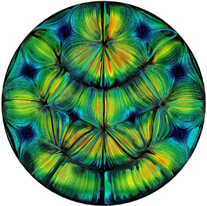
The analysis corresponding to the shallow liquid bridges with A = 0.17 is summarized in figures 7 and 8. In particular, the solution shown in figure 7(a) has been obtained starting from a diffusive temperature field and a quiescent state (zero velocity). In order to accelerate the emergence of convection, a horizontal acceleration has been used to temporarily perturb the initial state. Using this modus operandi, we have obtained the so-called CO pattern (named in this way by Borońska & Tuckerman (Reference Borońska and Tuckerman2010a,Reference Borońska and Tuckermanb)). The other three solutions in figure 7 have been produced using as initial condition a quiescent fluid, and perturbing the related diffusive temperature distribution via (4.1) with m = 4 (figure 7b), m = 5 (figure 7c) and m = 6 (figure 7d), respectively.
The pattern shown in figure 7(c) deserves special attention as it may be regarded as a PanAm with five rolls. Additional insights might be gathered through figure 8, where the flow streamlines have been reported. The presence of five main rolls can be observed in the centre of the liquid bridge with other four smaller rolls located on the sides (two for each side). Furthermore, a symmetry plane ideally cutting the liquid bridge into two parts can also be clearly identified.
4.2. Viscoelastic fluids and related oscillatory states
Having completed a sketch of the situation for buoyancy convection in liquid bridges of Newtonian fluids and having built a ‘reservoir’ of solutions to be used as initial conditions for the simulations dealing with non-Newtonian fluids, we now turn to the fully viscoelastic problem. In particular, we concentrate on the description of the SER regime, i.e. on values of θ for which we found oscillatory solutions (the steady states pertaining to the WER regime, which we could obtain for relatively small values of θ are not described as their properties are very similar to those of the solutions already discussed in § 4.1 for Newtonian fluids).
We wish to highlight that, for this regime, we further expanded the set of initial conditions (to be used to explore the response of these systems) by using a ‘forward and backward continuation’ strategy, that is, occasionally the final state provided by the simulation for a given value of the control parameter θ has been set as the initial condition for the next iteration (Kengne et al. Reference Kengne, Nguomkam Negou, Tchiotsop, Kamdoum Tamba, Kom, Kyamakya, Mathis, Stoop, Chedjou and Li2018; Lappa & Ferialdi Reference Lappa and Ferialdi2018a).
This means that the response of the system has been assessed with respect to three different categories of possible initial states, namely, perturbed thermally diffusive conditions, the multiple solutions corresponding to the final states of Newtonian fluids and the final velocity and temperature fields obtained for θ ≠ 0.
4.2.1. High aspect ratios
Following the same strategy undertaken in § 4.1, we follow a rational approach with situations of increasing complexity being examined as the discussion progresses. Accordingly, we start again from the simplest case, i.e. the liquid bridge with A = 1.
As shown in figure 9 (collecting all the results for this value of the aspect ratio), the oscillatory solutions obtained for Ra = 2000 and θ ≥ 0.1 can be represented in terms of frequency as a non-monotonic curve (the non-dimensional angular frequency being defined as 2π fL 2/α where f is the dimensional frequency of the temperature oscillation, and, as explained in § 2, L and α are the height of the liquid bridge and the fluid thermal diffusivity, respectively). These states correspond to standing waves with m = 1, as witnessed by the sequence of snapshots reported in figure 10.

Figure 9. Non-dimensional angular frequency ω (a) and (time-averaged) Nusselt number (b) as a function of the elasticity number θ for A = 1 and different values of Ra (the solid lines are spline fittings added as a guide for the eye: black line – Ra = 2000, blue line – Ra = 3000).

Figure 10. Three-dimensional streamlines (a–d) coloured according to the magnitude of the axial component of velocity (red and blue corresponding to rising and falling fluid, respectively) and three-dimensional isosurfaces (e–h) of non-dimensional azimuthal velocity wφ (four snapshots equally spaced in time within the oscillation period): standing wave with m = 1 (SW1) emerging for A = 1, Ra = 2000 and θ = 0.1.
As made evident by the distribution of streamlines (coloured by the magnitude of the non-dimensional axial component of velocity), the flow field essentially consists of a single horizontal roll that changes periodically its sense of rotation (from the anti-clockwise to the clockwise orientation and vice versa, while the direction of its axis remains fixed in space). In this regard, an interesting analogy could be established with the oscillatory solutions reported by Park (Reference Park2018) for rectangular cavities under the constraint of two-dimensionality. It can be seen that the two snapshots where the axial component of velocity displays maximum amplitude (panels a and c of the succession) are separated by intermediate states where such amplitude becomes almost negligible (panels b and d, respectively).
Following common practice used in earlier works dealing with Marangoni flows in liquid bridges, the distribution of the azimuthal component of velocity can also be used to provide useful information about this dynamics. As expected, the behaviour of this component is synchronous with that of the axial velocity; moreover, its nodes occupy fixed positions in space and change periodically their sign, giving the observer the illusion of a field that ‘pulsates’ in time (this feature has often been used in the existing literature on Marangoni flow as an useful means to distinguish standing-wave states from travelling waves, see, e.g. Lappa et al. Reference Lappa, Yasuhiro and Imaishi2003; Kang et al. Reference Kang, Wu, Duan, Hu, Wang, Zhang and Hu2019).
For Ra = 3000, however, the behaviour becomes more involved. The frequency curve is still non-monotonic. Moreover, though m = 1 is still the dominant spatial mode of convection over the entire range of considered values of θ, travelling waves emerge for θ ≤ 0.175 (while standing waves are recovered only for larger values of the elasticity parameter).
The classical signature of travelling waves can clearly be distinguished in figure 11. The aforementioned nodes of the azimuthal velocity (points where this velocity component attains a maximum or a minimum) do not occupy fixed positions. Rather they rotate continuously along the circumferential direction. Moreover, the intensity of these minima and maxima does not change in time (no temporal modulation of these extrema can be seen). The same behaviour can be recognized if the streamlines are examined. The axis of the horizontal roll undergoes a continuous rotation in the azimuthal direction while no variation can be seen in its strength. An external observer looking at figure 11 would get the illusion of a solid body rotating with a fixed angular velocity in the anticlockwise circumferential direction, which leads again to a notable analogy with the typical modes of spatio-temporal evolution revealed by earlier studies dealing with the Marangoni flow of Newtonian fluids in liquid bridges (see, e.g. Kang et al. Reference Kang, Wu, Duan, Hu, Wang, Zhang and Hu2019; in the following, we will refer to the ‘classical’ waveforms corresponding to standing and travelling waves as ‘SW’ and ‘TW’, respectively).

Figure 11. Three-dimensional streamlines (a–d) coloured according to the magnitude of the axial component of velocity (red and blue corresponding to rising and falling fluid, respectively) and three-dimensional isosurfaces (e–h) of non-dimensional azimuthal velocity wφ (four snapshots equally spaced in time within the oscillation period): travelling wave with m = 1 (TW1) emerging for A = 1, Ra = 3000 and θ = 0.1.
Interestingly, as evident in figure 9, regardless of whether the curve for Ra = 2000 or Ra = 3000 is considered, the frequency of oscillation of these solutions first increases as a function of the elasticity number and then it decreases when θ = 0.175 is exceeded.
This behaviour, which obviously cannot be regarded as an exclusive consequence of the transition from the TW to the SW (as it also holds for Ra = 2000 where no change in the prevailing waveform occurs), requires some justification.
Careful analysis of the structure of the flow field at Ra = 2000 for pre- and post-frequency-maximum values of θ has allowed us to discern that the above-mentioned non-monotonic trend should be regarded as the indirect outcome of the existence of a codimension-two point, i.e. two distinct branches of solutions (existing for the same value of Ra) which meet in proximity to the value of θ corresponding to the maximum of the combined curve. The related flow structures (shown in figure 12) simply reveal that the two families of solutions differ with respect to the symmetry properties of the velocity field. Before the codimension-two point, the azimuthal velocity component wφ is perfectly ‘anti-symmetric’ with respect to the midplane z = 1/2, i.e. wφ(z) = −wφ(1 − z) (see figure 12a), whereas after such a point the perfect antisymmetry is taken over by a solution for which wφ(z) ≠ −wφ(1 − z) (figure 12b). The different structure of the velocity field should be regarded as the root cause for the different properties of the two types of solutions (the ability to transport heat in the axial direction being smaller for the less symmetric solution, figure 9b) and the different frequency of oscillation (figure 9a).

Figure 12. Three-dimensional isosurfaces of non-dimensional azimuthal velocity wφ for A = 1 and Ra = 2000: (a) θ = 0.175, (b) θ = 0.3.
The results relating to the next aspect ratio, that is, A = 0.68 are summarized in figure 13. For this aspect ratio there is only one monotonic branch of solutions in the considered range of θ for each value of the Rayleigh number. In particular, the states at Ra = 2000 correspond to the curve with smaller value of the angular frequency. For the sake of conciseness, however, we do not show the related final fields (all exhibiting the same spatio-temporal behaviour, i.e. a standing wave with azimuthal wavenumber m = 2).

Figure 13. Non-dimensional angular frequency ω (a) and (time-averaged) Nusselt number (b) as a function of the elasticity number θ for A = 0.68 and different values of Ra (the solid lines are spline fittings added as a guide for the eye: black line – Ra = 2000, blue line – Ra = 3000).
On increasing the Rayleigh number to Ra = 3000, a very interesting set of solutions appears. Notably, we obtained this branch regardless of whether states with m = 1 and m = 2 were used as initial conditions. It deserves attention as it seems to escape a possible simple definition or classification in the frame of the classical models of standing or travelling wave. The related evolution in time (over a period of oscillation) can be gathered from figure 14.

Figure 14. Temperature distribution in the mid-height cross-section for A = 0.68, Ra = 3000 and θ = 0.175 (eight snapshots equally spaced in time within the oscillation period): two-breaking-rolls state with single (central) knot (BR2K(S)1).
Starting from figure 14(a), which represents a two-roll configuration, if one observes the evolution of this pattern (a–c), an evident pulsation can be recognized in the temperature distribution, which might be loosely interpreted as a standing wave. Indeed, initially (a), two hot spots and two cold spots, having comparable azimuthal extensions, can be recognized along the free surface of the liquid bridge. In figure 14(b), however, the two hot (east and west) spots disappear and an intermediate state is attained where the entire surface of the liquid bridge becomes apparently cold (while a hot area survives only in the centre). With time the size of this hot internal region decreases while two new hot spots nucleate on the free surface (north and south positions). In figure 14(c), these two hot spots have attained a size for which the system is in a thermal configuration with inverted colours with respect to that shown in panel (a). From figure 14(d), however, a new phenomenon occurs, i.e. the rolls start to break. Indeed, observing the pattern, two hot spots, each with azimuthal extension of approximately 90° located in proximity to the free interface can be seen. As time passes, these spots tend to grow in the radial direction. After some time (e) they merge and newly formed rolls appear with axis aligned along direction perpendicular to the original one. This becomes very evident by comparing panels (a) and (f).
The descriptions of this dynamics can be significantly simplified by introducing the concept of the knot (which will also prove very useful later for the characterization of phenomena much more complex than that reported in figure 14). We define it as the intersection point between the different prevailing directions displayed by the rolls during one cycle of oscillation. For A = 0.68 and Ra = 3000, these directions are perpendicular and the knot is perfectly in the centre of the liquid bridge. Remarkably, as shown in figure 14, the abovementioned hot spots formed in proximity to the interface tend to expand with time towards the knot (coincident with the centre of the liquid bridge in this case). In the following, we will therefore refer to this solution as a two-breaking-rolls (BR) state with a central single (stationary) knot (BR2K(S)1).
4.2.2. Intermediate aspect ratio
In this section, we concentrate on the cases with A = 0.34, for which we could get a number of fascinating phenomena. However, given the amount of qualitatively and quantitatively different results obtained by changing the initial conditions and allowing the elasticity number to span the interval from 0.1 to 0.2, the discussions reported in the following are not intended to be an exhaustive description of all these states (due to page limits), but rather to stimulate the interest of the reader in certain aspects, which we believe are particularly interesting. As already evidenced in § 4.1, these aspect ratios admit a significant number of multiple solutions.
In qualitative agreement with the results of the linear stability analysis for the infinite layer (see, e.g. Park & Lee Reference Park and Lee1996), the Nusselt number grows with both Ra and θ (figure 15b). As usual, we begin from the case with the smallest values of Ra and θ, i.e. Ra = 2000 and θ = 0.1. As sketched in figure 15, for this value of the elasticity number three different solutions coexist in the space of parameters. The first (not shown) is a centrally symmetric standing wave with m = 4 (in the legend of the figure 15 it is represented by the symbol ‘+’), originating from a thermally diffusive temperature field perturbed with an m = 4 disturbance (4.1). The second mode of convection is yet a centrally symmetric standing wave, with m = 4, obtained initializing the flow with a solution having m = 0, i.e. a purely axially symmetric mode. This state, can be regarded as an ‘alternate’ solution with respect to the other m = 4 mode, owing to its remarkably different frequency (see the symbol ‘×’ in figure 15a, the reader being also referred to figure 16 for the related spatio-temporal evolution).

Figure 15. Non-dimensional angular frequency ω (a) and (time-averaged) Nusselt number (b) as a function of the elasticity number θ for A = 0.34 and different values of Ra (the solid lines are spline fittings added as a guide for the eye: black line – Ra = 2000, blue line – Ra = 3000).

Figure 16. Temperature distribution in the mid-height cross-section (four snapshots equally spaced in time within the oscillation period): standing wave with m = 4 (A = 0.34, Ra = 2000 and θ = 0.1, simulation initialized with an m = 0 field).
A completely different solution (third possible mode of convection) can be produced if, as initial conditions, any of the following cases is considered: three rolls, a PanAm structure with m = 4, an m = 3 Mercedes pattern or a thermally diffusive state perturbed with an m = 2 centrally symmetric temperature disturbance (all these initial conditions leading the system to the same final state). In figure 15 this mode is represented with the symbol ‘Δ’ (see figure 17 for the related behaviour).

Figure 17. Temperature distribution in the mid-height cross-section (a–h) and corresponding streamlines coloured by the magnitude of the non-dimensional axial velocity (i–p). Eight snapshots equally spaced in time within the oscillation period are shown for A = 0.34, Ra = 2000 and θ = 0.1. This state (BR3K(S)2, i.e. a solution with three horizontal rolls and two primary stationary knots driving the related oscillatory dynamics) has been obtained assuming initial conditions corresponding to any of the following cases: three rolls, a PanAm structure with m = 4, an m = 3 Mercedes pattern or a thermally diffusive state perturbed with an m = 2 centrally symmetric temperature disturbance.
An adequate characterization of this third mode of convection is relatively difficult (requiring the introduction of new points of view and proper tools to describe the dynamics). The definition of new topological concepts relating to the structure of the pattern is particularly beneficial in this regard. Along these lines, we base part of our discussions on the idealized evolution shown in figure 18, assumed to model the sequence of events summarized in figure 17. In this figure, for simplicity, the rolls shown in figure 17(a) are sketched as perfectly parallel geometrical entities (figure 18a). Thereafter, we introduce three different types of characteristic ‘geometrical features’ required for a proper characterization of the patterning behaviour. The first simply corresponds to the main (primary) centre of pulsation for the temperature spots already introduced before as ‘knot’ and essentially located in proximity to the geometrical centre of the liquid bridge. Secondary and tertiary centres of attraction for the spots, however, also exist. As shown in figure 18, they are located near the lateral (circular) boundary. A symmetry plane that divides the liquid bridge into two parts can also be clearly identified.

Figure 18. Sketch of the behaviour shown in figure 17.
Starting from the situation shown in figure 17(a) (characterized by a three-roll configuration with two internal hot and cold temperature spots and two external spots of opposite sign, corresponding to figure 18a), as time increases, radial spokes are created (figure 17b) by which the two initial external spots (located at the free interface, one hot, one cold, each having an angular extension of 180°) are broken into disconnected regions (figure 17c). By virtue of this mechanism the initially hot (cold) spot located in the inner region of the liquid bridge is ‘transferred’ to the free surface in the form of two smaller hot (cold) spots separated by a spot of opposite sign (situation sketched in figure 18b).
As time increases, however, the two surface spots with the same colour (temperature) tend to move towards a common point of attraction located at the free interface (as shown in figure 17d). When they merge following the process sketched in figure 18(c), a situation that is mirror symmetric with respect to that shown in figure 17(a) is created (figure 17e corresponds to the situation sketched in figure 18d). The couple of peripheral hot (cold) spots have merged into a single region of the same temperature and the process can restart, giving rise to a new semi-cycle of oscillation (figure 17e–h). Following the same criterion already used to characterize the behaviour shown in figure 14, this state can therefore be identified as a BR3K(S)2, i.e. a solution with three horizontal rolls and two primary (stationary) knots driving the related oscillatory dynamics.
Interestingly, as made evident by figure 18, an observer taking a look at the flow in a section of the physical domain perpendicular to the symmetry plane highlighted in figures 18(a) and 18(d) would see rolls which periodically change their sense of rotation with a behaviour similar to that found by Park (Reference Park2018) for two-dimensional flow in square cavities.
If the value of θ is increased (yet for Ra = 2000) other interesting spatio-temporal behaviours can be produced with alternate mechanisms of breaking and merging of the disturbance spots and associated rolls.
For 0.125 ≤ θ ≤ 0.2, the branch represented by the symbol ‘Δ’ in figure 15 corresponds to the behaviour reported in figure 19 (this is the only stable state we could find for θ = 0.125 or 0.15 regardless of the used initial conditions). A second distinct branch, however, exists for 0.175 ≤ θ ≤ 0.2 (represented in figure 15 with the symbol ‘ $\diamondsuit $’ and originating from the m = 4 solution obtained for the Newtonian fluid used as initial condition).

Figure 19. Temperature distribution in the mid-height cross-section (eight snapshots equally spaced in time within the oscillation period): evolution mechanism (three breaking rolls with three rotating knots, i.e. BR3K(R)3) corresponding to the branch represented by the symbol ‘Δ’ in figure 15 (A = 0.34, Ra = 2000 and θ = 0.2).
Characterization of the patterning behaviour displayed in figure 19 on the basis of the same topological arguments used to describe figure 17 would be too difficult; therefore, we limit ourselves to highlighting that in this case the recognizable temperature spots apparently rotate in the azimuthal direction (with relatively small angular frequency, which increases with θ). This rotation, which can clearly be appreciated, e.g. by comparing figure 19(a) with figure 19(e), however, should not be confused with a classical travelling wave. While in travelling waves the rotation of the overall pattern can be ascribed to the continuous migration of disturbance nodes along the ring-shaped axis of a toroidal convective structure (giving the observer the illusion of a ‘rigid-body’ that rotates in space), in the present case the mechanism is much more complex as no underlying toroidal roll exists. Although the dynamics still produces the illusion of a pattern undergoing a solid-body rotation (in the counter-clockwise sense in figure 19), this effect results from the continuous rearrangement of rolls, which are continuously broken and reformed with orientation in space slightly shifted with respect to the earlier one. Therefore, the topological concept of knot is still applicable in this case. In particular, three knots exist (one for each couple of rolls). Owing to geometrical constraints (all the rolls have horizontal axis), in the cross-section these knots are approximately aligned along a line passing through the geometrical centre of the liquid bridge. As time increases, this line rotates in the azimuthal direction. This means that the apparent rotation of the pattern results from the continuous displacement in the azimuthal direction of purely topological features (unlike pure travelling waves where the same effect is produced by the displacement of disturbance nodes along a convective structure, which would otherwise be axisymmetric). For this specific mode of convection, we therefore coin the definition of ‘three breaking rolls with three rotating knots’ state (BR3K(R)3).
We can now analyse the second branch of solutions. The contours of the non-dimensional temperature field are illustrated in figure 20. Interestingly, the predominant pattern is the PanAm with m = 4.

Figure 20. Temperature distribution in the mid-height cross-section (eight snapshots equally spaced in time within the oscillation period): evolution mechanism (three breaking rolls with three ‘pulsating’ knots, BR3K(P)3) corresponding to the second branch shown in figure 15 (A = 0.34, Ra = 2000, θ = 0.2, simulation initialized with an m = 4 solution).
The PanAm pattern in the figure 20(a) starts evolving via a merging mechanism, which attracts two of the four hot spots originally located on the surface (figure 20a) towards the centre (figure 20b). Once the hot disturbance is mostly concentrated in the central region of the cross section of the liquid bridge, it starts to re-expand in the radial direction via the formation of extended patches which protrude from the centre towards the lateral boundary. This finally results in the re-emergence of four hot and four cold spots along the free interface (figure 20f) with reversed sign with respect to those visible in figure 20(a).
Unlike the case treated before, no apparent rotation can be recognized in this case. The previously discussed mechanism characterized by the continuous circumferential propagation of the knots is taken over by an alternate process in which the knots undergo a limited back and forth displacement along both the radial and azimuthal directions (three breaking rolls with three ‘pulsating’ knots, BR3K(P)3).
For Ra = 3000, the situation becomes even more complex. Indeed, three independent branches of solutions can be identified, i.e. a single branch spanning the interval 0.08 ≤ θ ≤ 0.2, an alternate mode existing for θ = 0.1 only and a third independent set of solutions occupying the range 0.15 ≤ θ ≤ 0.2.
The single solution existing for θ = 0.1 (symbol ‘![]() ’ in figure 15) has been found by initializing the simulation with the Newtonian solution with mode m = 3. The pattern spatio-temporal evolution is the same as that already shown in figure 19, which leads to the conclusion that this type of solution, not found for Ra = 2000 and θ = 0.1 tends to be selected by the system for relatively high values of θ and/or Ra.
’ in figure 15) has been found by initializing the simulation with the Newtonian solution with mode m = 3. The pattern spatio-temporal evolution is the same as that already shown in figure 19, which leads to the conclusion that this type of solution, not found for Ra = 2000 and θ = 0.1 tends to be selected by the system for relatively high values of θ and/or Ra.
The typical sequence of snapshots for the set of solutions corresponding to the symbol ‘○’ in figure 15 is illustrated in figure 21. This may be regarded as a variant of the behaviour already shown in figure 20 (although it is made more involved by the increased complexity of the mechanism by which the rolls periodically break and re-organize in time). Figure 22 finally presents the dynamics corresponding to the third branch of solutions for Ra = 3000 (indicated by the symbol ‘ $\bullet$’ in figure 15). These states have been obtained initializing the flow with a three-roll state.

Figure 21. Temperature distribution in the mid-height cross-section (eight snapshots equally spaced in time within the oscillation period): evolution mechanism corresponding to the symbol ‘○’ in figure 15 (A = 0.34, Ra = 3000, θ = 0.1). This state has been obtained assuming initial conditions corresponding to any of the Newtonian flow solutions shown in figure 6, with the only exception of the m = 3 case.

Figure 22. Temperature distribution in the mid-height cross-section (12 snapshots equally spaced in time within the oscillation period): evolution mechanism (BR3K(R)2) corresponding to the symbol ‘$\bullet$’ in figure 15 (A = 0.34, Ra = 3000, θ = 0.2, simulation initialized with a three-roll solution).
Interestingly, pattern formation and evolution in this case are very similar to those already presented in figure 17. A distinguishing mark, however, can be found in the visible rotation undergone by the knots, which can easily be observed by comparing, for instance, figure 22(a,c,e,g,i,k).
It is worth remarking once again that this rotation is a topological feature displayed by a pattern with dominant horizontal vorticity. Therefore, it should not be confused with a travelling-wave mode such as that obtained for A = 1 and Ra = 3000 (figure 11).
4.2.3. Shallow liquid bridge
This final section is devoted to discussing the last of the aspect ratios examined in this study, i.e. the shallow liquid bridge with A = 0.17. Given the extremely high computational cost of these simulations (each requiring several weeks) such analysis has been limited to three values of the elasticity number only (namely, θ = 0.1, 0.15 and 0.2).
As shown in figure 23, the Nusselt number still displays an increasing trend when its dependence on the elasticity number is considered. Simulations, initialized with the two-torus or the CO solutions shown in figure 7, however, have led to the identification of two possible states.

Figure 23. (Time-averaged) Nusselt number as a function of the elasticity number θ for A = 0.17 and Ra = 2000.
The typical dynamics for θ = 0.1 is illustrated in figures 24 and 25.

Figure 24. Temperature distribution in the mid-height cross-section (eight snapshots equally spaced in time within the oscillation period, A = 0.17, Ra = 2000, θ = 0.1, simulation initialized with the ‘CO’ or the two-torus solution).

Figure 25. Three-dimensional isosurfaces of non-dimensional azimuthal velocity (eight snapshots equally spaced in time within the oscillation period, A = 0.17, Ra = 2000, θ = 0.1, simulation initialized with the ‘CO’ or the two-torus solution).
The pattern features the apparent continuous creation of localized regions with different temperatures. Unlike the classical pulsating behaviour of standing waves where such regions occupy fixed positions in space while the related temperature switches continuously from cold to hot (and vice versa), in the present case these differently coloured areas show a rhythmic displacement in time, which occasionally results in coalescence events (merging of spots with the same colour) or spot rupture (leading to disconnected spots of the same sign).
This peculiar spatio-temporal mechanism may be regarded as a clear distinguishing factor with respect to both classical standing and travelling waves. Spots do not shrink and then expand as a function of time as they would do in the case of a standing wave. They do not rotate about the axis of the liquid bridge either.
Though a first glimpse of their behaviour may give the observer the illusion of a set of almost independent islands wandering in the sea, similar to those identified by Lappa & Ferialdi (Reference Lappa and Ferialdi2018a) as the ultimate state of chaotic viscoelastic Marangoni–Bénard convection, a more focused analysis of their peculiar dynamics reveals the hidden order which governs their evolution. Yet a series of knots exist which determine locally the evolution of the thermofluid-dynamic field in a certain neighbourhood of their position. In a given area surrounding these topological centres, temperature spots undergo apparently complex dynamics, which reflects the rupture of rolls initially having a given direction and flow reorganization to form new rolls with a different orientation (mainly perpendicular to the original one). This continuous re-organization of the pattern occasionally leads to the formation of rolls displaying a spiralling configuration (e.g. figure 24a).
Despite the occasional emergence of these textures, however, no ‘ensemble’ scheme or simply definable spatio-temporal behaviour can be recognized in this case. No special points exist in the pattern which could be uniquely identified through the topological order of the radial spokes which originate from them.
Surprisingly, the solution emerging for θ = 0.15 and θ = 0.2 looks more regular (figures 26 and 27). In this specific case, the lines bounding the temperature spots organize themselves to form a typical network that evolves in time following a recognizable scheme. Starting from a condition with six almost-parallel rolls (figure 26a), the flow evolves towards a 3-torus configuration (figures 26b and 26c) with the two inner tori displaying centrally symmetric m = 4 disturbances and the external one taking an almost unperturbed (axisymmetric) shape. The resulting pattern is similar to the so-called ‘target’ states revealed by earlier studies about steady or oscillatory RB convection in Newtonian fluids. Despite this analogy, the present findings, however, are remarkably different. While for classical RB convection in Newtonian fluids, oscillatory target patterns reduce to radially propagating rings of concentric rolls (referred to as axisymmetric travelling waves; Croquette et al. Reference Croquette, Mory and Schosseler1983; Tuckerman & Barkley Reference Tuckerman and Barkley1988; Siggers Reference Siggers2003), in the present case this configuration is just a temporary or intermediate state, as it is quickly taken over again by parallel rolls as time increases. These reappear in figure 26(d) rotated by 90° with respect to the direction visible in figure 26(a) and then undergo a new cycle of evolution as shown in figures 26(e) to 26(h), which may be regarded as the mirror image of that shown in figure 26(a–d) in terms of colour of the temperature spots (reversed sign of the temperature disturbances). The most striking feature of this solution is therefore its ability to jump continuously from situation where axial vorticity is dominant to situations in which this role is taken over by horizontal vorticity and so on.

Figure 26. Temperature distribution in the mid-height cross-section (eight snapshots equally spaced in time within the oscillation period, A = 0.17, Ra = 2000, θ = 0.15, simulation initialized with the two-torus solution): (a), (f) and (h) correspond to a 6-rolls state while (b), (c), (g) and (h) may be seen as a perturbation with m = 4 superimposed on a 3-torus state with the torus closest to the free surface being almost axisymmetric.

Figure 27. Three-dimensional isosurfaces of non-dimensional azimuthal velocity (eight snapshots equally spaced in time within the oscillation period, A = 0.17, Ra = 2000, θ = 0.15, simulation initialized with the two-torus solution).
For the convenience of the reader, all the spatio-temporal mechanisms discussed in this section have finally been grouped into a single figure in order to produce a meaningful map of the observed regimes in the parameter space (Ra, θ, A) (figure 28). Although no classification is perfect, and it is hard to distillate a precise definition from an observation, in particular, the following acronyms have been used to capture the essential aspects of the observed phenomena: SW (classical standing wave), TW (classical travelling wave), BRK (states with rolls which break and reform with the time-varying topology governed by the existence of ‘knots’). Moreover, the following information has also been included in the related labels: for the states with prevailing axial vorticity, the integer (appearing just after the text ‘TW’ or ‘SW’) is the classical azimuthal wavenumber m, while the integers n and N following ‘BR’ and ‘K’, respectively, are the number of horizontal rolls and the number of primary knots governing the dynamics of oscillatory modes with dominant horizontal vorticity (for these cases, for the sake of completeness, additional information is reported inside parentheses in the form of a single letter (‘S’, ‘P’ or ‘R’) to indicate the prevailing apparent behaviour (stationary, pulsating or rotating, respectively) of the primary knots).

Figure 28. Legend: standing wave, SW; travelling wave, TW; rolls that periodically break and reform in time with a new orientation in space, BR; the integer m (appearing just after the text ‘TW’ or ‘SW’, in the areas with the blue background) is the classical azimuthal wavenumber for the states with prevailing axial vorticity (toroidal rolls), while the integers n and N following the labels ‘BR’ and ‘K’, respectively, are the number of horizontal rolls and the number of primary knots governing the related oscillatory dynamics. In the case of oscillatory modes with dominant horizontal vorticity (red background), additional information is reported inside round parentheses in the form of a single letter (‘S’, ‘P’ or ‘R’) to indicate the prevailing apparent behaviour (stationary, pulsating or rotating, respectively) of the primary knots.
On the basis of this conclusive map, some interesting general trends can be recognized. In fact, it can be seen that the classical standing and travelling waves (resembling those observed in earlier studies dealing with the companion problem of Marangoni flow in liquid bridges, Lappa Reference Lappa2009; Kang et al. Reference Kang, Wu, Duan, Hu, Wang, Zhang and Hu2019) are favoured for higher values of the aspect ratio and a smaller level of elasticity (low θ); vice versa, the oscillatory mechanisms with breaking rolls become dominant as θ grows and/or the aspect ratio is decreased. The magnitude of the Rayleigh number has also a non-negligible impact on this scenario. On increasing Ra from 2000 to 3000, solutions of the BR type can be found also for relatively high values of A (0.68) (whereas for Ra = 2000 their existence is possible only for A ≤ 0.34), which indicates that the region of existence of the states with prevailing horizontal vorticity spreads over higher values of A as Ra grows. Moreover, for Ra = 3000, the following sequence of changes takes place on decreasing the aspect ratio of the liquid bridge: the SW and TW solutions existing for A = 1 are completely replaced by BR modes of convection with stationary knots for A = 0.68; if the aspect ratio is decreased further, knots no longer occupy fixed positions in space and start to oscillate back and forth in space along a well-defined direction ((P) states) or apparently rotate in the azimuthal direction ((R) states).
As a very final testbed, in order to assess the asymptotic behaviour of these systems in the limit as the aspect ratio of the liquid bridge tends to zero, we have considered the case of a horizontally extended layer of viscoelastic fluid delimited from above and from below by solid walls. In particular, the numerical simulations have been conducted assuming a physical domain with horizontal extension 15 times the depth and periodic boundary conditions at the lateral boundaries (in order to mimic the behaviour of a fluid domain with infinite extent). The simulations for Ra = 2000 and θ = 0.1 are shown in figure 29.

Figure 29. Rayleigh–Bénard convection in a layer of viscoelastic fluid delimited by horizontal solid walls, heated from below and cooled from above (snapshots of the isosurfaces of the vertical component of velocity evenly distributed over the oscillation period, 15 × 15 × 1 domain with top and bottom solid walls and periodic lateral boundary conditions, β = 1/2, Prg = 8, Ra = 2000, θ = 0.1, elasticity number defined as θ = αλ/d 2 where d is the depth of the layer, non-dimensional angular frequency of oscillation  $\omega \cong 7.9$,
  $Nu \cong 1.11$; 675 000 grid points).
It can be seen that in the limit as the horizontal extension of the domain becomes infinite, the mechanism with rolls that break and reform with a direction that is rotated with respect to the original one becomes the norm. States with rolls extending along the x or y direction (panels (a), (e) or (c), (g) in figure 29, respectively) are interspersed with ‘checkerboard’ patterns where no clear direction can be identified (panels (b), (d), (f) and (h)). Cross-comparison of panels (a) and (e) (or in an equivalent way of panels (c) and (g)) also leads to the conclusion that rolls periodically oriented along a given direction also change regularly their sense of rotation (from the clockwise to counter-clockwise sense and vice versa). From these figures, it can also be inferred, that the rotation angle becomes exactly 90° in the asymptotic condition as the aspect ratio of the system tends to zero (compare e.g. figure 29a and c).
This observation is particularly meaningful as it also leads to natural conclusion that the aforementioned transient ‘target’ states revealed by the simulations for A = 0.17 and θ = 0.15 and θ = 0.2 should be regarded as the consequence of rolls (emerging with direction rotated by 90° with respect to their previous orientation) to bend in order to fit into the cylindrical physical domain delimited externally the free surfaced of the liquid bridge.
5. Discussion
Additional insights into all these behaviours can be gathered from the iso-surfaces of the azimuthal velocity component shown in figures 25 and 27. Besides the details being provided about the three-dimensional structure of the flow itself, these figures are also instrumental in clarifying what sets these convective modes apart with respect to other typical oscillatory instabilities of the RB in Newtonian fluids in shallow domains.
The latter have been largely investigated resorting to the assumption of infinite layer for various liquids and circumstances. In the present section, it is worth recalling that a summary of the related stability behaviour can be represented using the so-called Busse balloon (Busse Reference Busse1967; Busse & Whitehead Reference Busse and Whitehead1971, Reference Busse and Whitehead1974; Busse & Clever Reference Busse and Clever1979; Clever & Busse Reference Clever and Busse1989, Reference Clever and Busse1993, Reference Clever and Busse1994; Lappa Reference Lappa2009), which also provides useful indications on the nature of the emerging flows. These instabilities have been classified according to the prevailing spatio-temporal behaviour as skewed–varicose, travelling wave, cross-roll, bimodal, zig-zag, etc. In the following, however, we will content ourselves with highlighting the differences with respect to the present dynamics (the reader interested in a more thorough discussion of these classical instabilities should consult the relevant references cited hereafter).
The simplest way to begin this discussion, perhaps, is to start from the realization that the formation of new rolls with a direction perpendicular to the original set of rolls is not an exclusive prerogative of viscoelastic RB convection.
As an example, the classical cross-roll instability of RB in Newtonian fluids manifests itself as a modulation of the pattern parallel to the axes of the initial rolls. This instability typically causes a perturbation responsible for the emergence of rolls growing perpendicularly to the original pattern of rolls (Busse & Whitehead Reference Busse and Whitehead1971). In some circumstances, this mode of convection can produce localized defects in the form of ‘totem’ structures, relatively similar in appearance to some of the features visible in figures 24 or 26. In general, however, for Rayleigh numbers not too far above the critical value, the growth of the perpendicular rolls and the concurrent decay of the original rolls proceeds until the original rolls are completely taken over by the perpendicular or cross-rolls (Busse & Whitehead Reference Busse and Whitehead1971). Moreover, the new formed pattern is essentially a steady one.
For higher values of the Rayleigh number (of the order 2 × 10⁴), the cross-roll flow in Newtonian fluids naturally evolves into another form of stationary flow known as ‘Bimodal’ convection (Busse & Whitehead Reference Busse and Whitehead1974) where steady boundary-layer-type structures appear (Clever & Busse Reference Clever and Busse1994 studied this form of convection for 10 ≤ Pr ≤ 100). As originally shown by Busse (Reference Busse1967), this instability originates from the thermal boundary layers at the rigid upper and lower boundaries of the fluid layer; in fact, the additional small-wavelength convection rolls that develop at right angle to the basic roll are particularly suited to take advantage of the buoyancy stored in these areas. In this case the original rolls and the secondary set of perpendicular rolls induced by the instability clearly coexist in the same physical space. A typical feature of this type of convection is the striking similarity between its patterns and a two-dimensional crystal lattice (although this similarity includes various kinds of irregularities found in the lattice such as edge dislocations, these patterns, however, do not look like the structures shown in figures 24 and 26).
Another instability mechanism known for RB in Newtonian fluids is the so-called knot instability. According to the classical Busse balloon, the predominant modes at high Ra are bimodal convection at large Prandtl numbers (Pr ≥ O(10)), knot convection at moderate Prandtl numbers (O(1) < Pr < O(10)) and travelling (or standing) waves in low-Pr fluids (Pr ≤ O(1)). The knot instability (yet a stationary bifurcation) breaks the same symmetries as the cross-roll one, but with a much smaller value of the wavenumber along the axis of the rolls. For Ra > 3 × 10⁴ strong plumes are typically created as thermal features embedded into the currents of rising and descending liquid. At the same time, ‘streamers’ evolve in the thermal boundary layers feeding the plumes. These features look like knots in the shadowgraph observations of convection (Busse & Clever Reference Busse and Clever1979; Clever & Busse Reference Clever and Busse1989), which provides a justification for the name used for this instability (which, however, has nothing to do with the concept of knot as it has been used in § 4 of the present study). These nearly axisymmetric plumes display an increased efficiency in transporting heat with respect to rolls for intermediate values of the Prandtl number (Pr ≤ 7). While bimodal convection is the preferred state of convection at high Prandtl numbers, knot convection assumes this role in the range 2 ≤ Pr ≤ Pr*, where Pr* increases from approximately 10 at a Rayleigh number of the order 3 × 10⁴ to much higher values as Ra grows (Busse & Clever Reference Busse and Clever1979).
As the reader might have realized at this stage, all these secondary states of RB convection display some interesting analogies or similarities with the states described in the preceding pages. Nevertheless, it should be pointed out that all these convective modes are essentially stationary (with the exception of travelling waves, which will be discussed at the end of this section). Moreover, they typically exist in regions of the space of parameters characterized by much higher values of the Rayleigh number with respect to those considered here (they are indeed, secondary modes of convection, i.e. states attained when a second threshold is exceeded after the first one leading the fluid from quiescent conditions to steady parallel rolls). A similar concept applies to the so-called ‘spoke’ pattern convection. This name was coined by Busse & Whitehead (Reference Busse and Whitehead1974) to describe the time-dependent (tertiary) form of convection emerging in layers of Newtonian fluids heated from below when the Rayleigh number exceeds a value of the order 3 × 10⁴ for Pr ≥ O(1). For such conditions, the thermal boundary layers located in proximity to the top and bottom walls become unstable and erupt sheets of hot and cold fluid moving radially inward toward central plumes which carry fluid to the opposite boundary. This results in the appearance of radial ‘spokes’, which can be visualized experimentally with the shadowgraph method.
Spoke pattern convection is typically produced as a tertiary mode of convection via the instability of bimodal or knot convection. From a physical point of view, the related mechanisms of transition are rather similar in that the emergence of hot and cold blobs from the hot and cold boundary layers is the main reason for the transition from steady to time-dependent convection (Clever & Busse Reference Clever and Busse1993, Reference Clever and Busse1994).
Given these premises, we can now come back to the results presented in figures 25 and 27 and use them to highlight the differences between the kind of spoke pattern convection shown in figures 24 and 26 and the classical spoke pattern RB convection originally investigated by Busse and co-workers.
By inspecting the isosurfaces in figures 25, 27 and 29, indeed, it becomes evident that no boundary layers exist near the top and bottom disks (which, among other things is consistent with the relatively small values of the Rayleigh number assumed in our study; indeed, let us briefly recall that the thickness of thermal boundary layers in RB convection is expected to scale as Ra −1/4, see, e.g. Lappa (Reference Lappa2011) and references therein). The oscillatory states found in the viscoelastic fluid, therefore, cannot be ascribed to boundary-layer-driven phenomena.
Some room should finally be devoted to examining the relationship between the present dynamics and the travelling-wave states predicted by the Busse balloon as secondary modes of convection for Pr = O(1). Some relevant information along these lines for the case of enclosures with the cylindrical symmetry can be found in the study by Boronska & Tuckerman (Reference Boronska and Tuckerman2006), who considered Rayleigh–Bénard convection in the parameter region of 0.318 ≤ A ≤ 0.345 for Pr = 1 and adiabatic lateral (solid) wall. According to their numerical investigation, the primary axisymmetric convective state loses stability to an m = 3 perturbation via a Hopf bifurcation. In particular, these authors found long-lasting standing waves which were eventually taken over by travelling waves (on increasing the time or the applied Rayleigh number).
In the light of all these arguments, it can be concluded that none of the classical secondary or higher-order modes of RB convection known for the case of Newtonian fluids can directly be applied to interpret the dynamics of viscoelastic RB convection in liquid bridges.
Having completed a sketch of the differences between the primary and secondary states of RB convection for Newtonian fluids and the corresponding modes obtained for a viscoelastic liquid bridge heated from below, in the second part of this section, we change direction completely and turn to identifying possible ‘similarities’ with other types of viscoelastic flow, i.e. aspects that are shared among the different areas of thermogravitational, thermocapillary and rotating fluids and, therefore, can be said to ‘unify’ the study of these subjects (the reader being also referred to the interesting point of view elaborated by Larson Reference Larson1992).
Along these lines, we start from the simple and meaningful remark that overstability seems to be a common property of different kinds of flow, including those where no thermal effects are involved such as Taylor–Couette systems (TCS). Taylor–Couette flow is a classical subject in fluid dynamics. It corresponds to the motion of a fluid encapsulated in the annular gap between two concentric cylindrical walls rotating at different velocities (typically, the outer wall is held fixed while the inner cylinder rotates at a constant angular velocity). If Newtonian fluids are considered, it is known that by increasing the Reynolds number (Re), at a certain stage, the initial purely azimuthal flow is taken over by a more complex (still stationary) flow structure featuring toroidal vortices with unit aspect ratio (i.e. radial extension comparable to the extension along the axis of the cylinder). This instability is of centrifugal nature (owing to the rotating inner cylinder introducing a large negative radial gradient of angular momentum into the flow, the flow tends to redistribute the angular momentum via viscous diffusion if the flow inertia is sufficiently small, or by nonlinear advection for larger flow inertia). For a further increase in Re, various types of waves can be excited (the reader being referred to Lappa (Reference Lappa2012) for an extensive review of studies produced over the years on this subject and a map of the related possible spatio-temporal states).
Notably, the existing work on this type of flow in viscoelastic fluids has concentrated on two extremes, which may be regarded as the analogues of the WER and SER regimes coined by Li & Khayat (Reference Li and Khayat2005) to classify the possible states of RB convection. For TCS a first branch of solutions exists for high values of the Reynolds number and weak levels of elasticity (displaying a bifurcation picture very similar to those already known for Newtonian fluids). It is followed by a second branch obtained for high levels of elasticity and vanishing Reynolds number. In the latter case, purely elastic oscillating vortices have been observed in typical experiments (see, e.g. Muller, Shaqfeh & Larson Reference Muller, Shaqfeh and Larson1993) to emerge directly from the initial purely azimuthal flow. As elasticity exceeds a critical level, the flow field undergoes transition from the purely azimuthal (steady) flow to a time-dependent (oscillatory) state via a subcritical bifurcation similar to that affecting viscoelastic RB convection (see, e.g. Rosenblat Reference Rosenblat1986). As already discussed in the introduction, the two above-mentioned WER and SER regimes of RB convection correspond to weakly elastic and strongly elastic fluids, respectively. A weakly (strongly) elastic fluid is identified as a fluid with elasticity number θ < θh (θ > θh), where θh is the critical elasticity number for the onset of oscillatory convection (Hopf bifurcation) and the transition to oscillatory convection occurs in the post-critical (pre-critical) range of the Rayleigh number (Li & Khayat Reference Li and Khayat2005). As argued by several authors, such a similarity in the phenomenology displayed by RB convection and TCS suggests ‘that the mechanism for overstability may be common to both flow contexts’ (Li & Khayat Reference Li and Khayat2005).
Along these lines, in the present work, additional computations (besides those illustrated in § 4) have been conducted for θ ≥ 0.1 and increasing values of Ra located under the threshold value needed for the onset of RB convection in liquid bridges of Newtonian fluid (sub-critical range). These simulations (not shown for the sake of brevity) have confirmed that for all the considered cases, the system evolves directly from a quiescent thermally diffusive state to an oscillatory solution, which clearly indicates that the considered bifurcation should be considered a classical example of overstability, i.e. a Hopf bifurcation of the same nature of that reported by Martínez-Mardones & Pérez-Garcíıa (Reference Martínez-Mardones and Pérez-Garcíıa1990) for the rigid-rigid case and parameters (and a viscoelastic model) similar to those considered in the present work (a subcritical Hopf bifurcation).
In the present section, towards the end to put the results discussed in § 4 under a more general perspective, we pursue the analogy between RB and TCS even further by expressly pointing out that the latter has been the first type of flow for which the role played by elasticity in increasing the number of multiple solutions has somehow been recognized experimentally. The ability of this type of flow to give rise to multiple possible states in the space of phases for a fixed value of the Reynolds number had already been identified for Newtonian fluids since the original work by Coles (Reference Coles1965). Remarkably, other authors (Muller et al. Reference Muller, Shaqfeh and Larson1993) have shown experimentally that this ability is even enhanced when elasticity enters the dynamics and the interaction among multiple solutions can produce quick progression to chaos. For related numerical results based on LSA, the reader may consider Northey, Armstrong & Brown (Reference Northey, Armstrong and Brown1992) where the flatness of the neutral stability curve with respect to changes in axial wavenumber was discussed as a possible source of nonlinear interactions between families of time-periodic states that are closely spaced with respect to the value of the elasticity parameter. Northey et al. (Reference Northey, Armstrong and Brown1992) also showed by means of nonlinear (finite element method) simulations that standing waves tend to be the preferred mode of convection for TCS (see also by Larson Reference Larson1992), which may be regarded as another analogy with some of the dynamics described in the present study (figure 10).
The literature about viscoelastic RB has been already discussed in the introduction and is not reported here to avoid duplications (relevant examples of nonlinear studies about the emerging planforms or waveforms being Martínez-Mardones et al. Reference Martínez-Mardones, Tienmann, Walgraef and Zeller1996; Parmentier et al. Reference Parmentier, Lebon and Regnier2000; Li & Khayat Reference Li and Khayat2005).
Subcritical instabilities and overstability are also a property of Marangoni–Bénard (MB) convection (Lebon et al. Reference Lebon, Parmentier, Teller and Dauby1994). Unfortunately, only a few analyses have been devoted to the investigation of viscoelastic MB flow taking into account nonlinear effects. Here, we limit ourselves to discussing briefly the main outcomes of the studies by Parmentier et al. (Reference Parmentier, Lebon and Regnier2000) and Lappa & Ferialdi (Reference Lappa and Ferialdi2018a), as relevant exemplars for the WER and SER, respectively. Most interestingly, the former authors could show that the so-called inverted ‘hexagonal cells’ (convection with fluid motion downward at the centre of the cells), which for Newtonian fluids are known to be possible only in liquid metals (or other fluids with small value of the Prandtl number) can become a stable mode of convection in the WER regime of MB flow. Lappa & Ferialdi (Reference Lappa and Ferialdi2018a) concentrated on the SER illustrating that on increasing the level of elasticity of the considered fluid for a fixed value of the Marangoni number (Ma), classical MB convection characterized by polygonal cells all rigidly embedded in a crystalline texture (side-by-side arrangement) is taken over by an unsteady mode of convection where cells lose their original well-defined boundary and acquire a rounded shape. In such a new regime cells are separated by intermediate regions of more or less motionless fluid (referred to as ‘buffer’ areas in Lappa & Ferialdi Reference Lappa and Ferialdi2018a), which allow them to move back and forth along uncorrelated horizontal directions. As a result, ‘like islands wandering in the sea’ cells undergo occasional coalescence or splitting phenomena (thereby resembling a behaviour qualitatively similar to that shown in figures 24 and 25). This specific behaviour led these authors to refer to these cells with the name of ‘oscillons’, loosely used to indicate a kind of excitations emerging as localized time-dependent convective structures in an otherwise uniform background. Multiple solutions were found to be a typical feature of MB convection as well (their ultimate manifestation being the existence of such oscillons).
In the light of the above considerations for these different forms of convection, it becomes evident that the common ability of all these flows to give rise to unsteady patterns of increasing complexity as the level of elasticity increases reflects some common ‘physics’. While for classical Newtonian fluids, transition from steady to time-dependent states generally requires an increase in the magnitude of the driving force and/or a decrease in the intensity of viscous forces (namely, an increase in Re, Ra or Ma for TCS, RB and MB convection, respectively), for viscoelastic fluids time dependence can be obtained by increasing the level of elasticity while Re, Ra or Ma are kept constant (which is exactly what has been observed in the present work). From a practical standpoint, the most relevant way to elucidate the significance of this observation and understand the related physical implications is to consider the dichotomy introduced by Groisman & Steinberg (Reference Groisman and Steinberg1998, Reference Groisman and Steinberg2000) to distinguish inertial and elastic instabilities in fluid flow.
This simple concept can be used to build an interesting unifying interpretation for this dynamics based on the ability of these fluids to retain stresses even when no gradient of velocity is present.
It can be argued that if stretching of the polymer molecules present in the liquid is produced by an initial flow, these molecules will relax with a characteristic time that does not match that of the flow that has produced their deformation. Accordingly, these molecules will be able to perturb the flow producing secondary flows able to stretch them even further. It is in this way that initially small disturbances can be amplified. Remarkably, since this internal feedback loop does not need inertia, centrifugal forces or other types of disturbances produced by thermal buoyancy or surface-tension effects, it is universal and can occur even in the limit as the aforementioned characteristic numbers tend to zero (Groisman & Steinberg Reference Groisman and Steinberg1998, Reference Groisman and Steinberg2000). This might be seen as a still relevant physical interpretation supporting the very complex regimes of RB convection identified in the present work for relatively small values of the Rayleigh number.
As a concluding remark for this section, we wish to highlight that a future direction of research might be represented by the need to clarify if some universality classes can also be identified with respect to the route towards chaos. Indeed, some existing studies have provided some evidence that for viscoelastic flows characterized by multiple solutions (the reader being referred to Muller et al. Reference Muller, Shaqfeh and Larson1993; Li & Khayat Reference Li and Khayat2005; Lappa & Ferialdi Reference Lappa and Ferialdi2018a, for TCS, RB and MB systems, respectively) a possible common path of evolution might be represented by the so-called Curry–Yorke scenario (originally introduced by Curry & Yorke (Reference Curry, Yorke, Markley, Martin and Perrizo1977) to indicate direct transition from quasi-periodic solutions, i.e. a T 2 torus to fully turbulent states). Addition investigations will be required to verify the validity and generality of this statement, which might also be considered as a possible hint for the continuation (extension) of the present study.
6. Conclusion
At present there are no published papers examining numerically the dynamics of viscoelastic RB convection in three-dimensional geometries with cylindrical symmetry; hence, this is the first time that detailed data on the flow phenomenology and its relationship with typical parameters have been presented.
As revealed by the present analysis, RB convection in viscoelastic liquid bridges inherits peculiar features, which, on the one hand, are typical of RB convection in Newtonian fluids (namely, its tendency to produce multiple states of convection) and, on the other hand, reflect ‘typical’ properties of viscoelastic fluids (the so-called ‘overstability’). The combination of these two peculiar features results in a kaleidoscope of possible states, some of which exist in parallel in the space of parameters while others are ‘unique’. Typical solutions include (but they are not limited to) classical standing waves and travelling waves (for relatively high values of the aspect ratio), and alternate (heretofore unseen) modes of convection (for relatively shallow liquid bridges) that seem to escape a relatively simple definition in the frame of existing criteria or earlier studies about the dynamics of oscillatory RB convection in Newtonian fluids. A general property of these alternate states is the unusual ability to break an existing set of rolls into smaller convective structures that subsequently merge causing a variation in the prevailing direction of the axis of rolls with respect to the preceding state. This property can manifest itself globally (affecting the entire pattern with an abrupt change in the dominant direction of parallel rolls) or locally (in the neighbourhood of special points that we have called knots). In the latter case different types of behaviours can be produced depending on whether these knots are fixed in space, travel continuously in the azimuthal direction or undergo back and forth motion along certain directions. Both states with dominant axial vorticity or horizontal vorticity are possible, though a net distinction between these two categories of flow is not possible since solutions also exist where the flow continuously jumps from modes with central symmetry to parallel rolls.
Future studies shall be devoted to examining the case of hybrid buoyancy–Marangoni convection in viscoelastic liquid bridges for which no information has been produced till date.
Acknowledgements
This work has been partially supported by the UK Engineering and Physical Sciences Research Council (EPSRC grant EP/R043167/1).
Conflicts of interest
The author reports no conflict of interest.


