1 Introduction
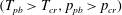
The operating pressure of propulsion and energy systems, such as gas turbines, liquid rocket engines or supercritical water-cooled reactors, is continuously increasing to improve performances. As a result, the working fluid often reaches pressures and temperatures exceeding critical values,
 $p>p_{cr}$
and
$p>p_{cr}$
and
 $T>T_{cr}$
, respectively, hence achieving a supercritical state. While promoting high heat transfer rates and thermodynamic efficiencies and suppressing detrimental interfacial effects commonly found in low-pressure boiling or cavitation processes (Zhong et al.
Reference Zhong, Fan, Yu, Li and Sung2009; Zhang et al.
Reference Zhang, Liu, Dong and Zhao2011; Wen & Gu Reference Wen and Gu2011), the heightened coupling between pressure, temperature and density in the supercritical regime also accentuates unwanted fluid dynamic instabilities such as thermoacoustic oscillations in injection systems (Casiano, Hulka & Yang Reference Casiano, Hulka and Yang2010) or in fuel heat exchangers (Thurston Reference Thurston1964; Palumbo Reference Palumbo2009; Wang et al.
Reference Wang, Zhou, Pan and Wang2015), the latter often leading to catastrophic hardware failure if uncontrolled. These so-called real fluid effects are intensified in near-critical conditions,
$T>T_{cr}$
, respectively, hence achieving a supercritical state. While promoting high heat transfer rates and thermodynamic efficiencies and suppressing detrimental interfacial effects commonly found in low-pressure boiling or cavitation processes (Zhong et al.
Reference Zhong, Fan, Yu, Li and Sung2009; Zhang et al.
Reference Zhang, Liu, Dong and Zhao2011; Wen & Gu Reference Wen and Gu2011), the heightened coupling between pressure, temperature and density in the supercritical regime also accentuates unwanted fluid dynamic instabilities such as thermoacoustic oscillations in injection systems (Casiano, Hulka & Yang Reference Casiano, Hulka and Yang2010) or in fuel heat exchangers (Thurston Reference Thurston1964; Palumbo Reference Palumbo2009; Wang et al.
Reference Wang, Zhou, Pan and Wang2015), the latter often leading to catastrophic hardware failure if uncontrolled. These so-called real fluid effects are intensified in near-critical conditions,
 $p\sim p_{cr}$
and
$p\sim p_{cr}$
and
 $T\sim T_{cr}$
, which will be examined by the present paper in the context of turbulent heat and mass transfer in a canonical compressible turbulent channel flow setting.
$T\sim T_{cr}$
, which will be examined by the present paper in the context of turbulent heat and mass transfer in a canonical compressible turbulent channel flow setting.
The lay understanding is that supercritical fluids share properties of both gases and liquids, in a seemingly homogeneous yet ambiguous state of matter. In reality, there is an identifiable transition between pseudoliquid (or liquid-like) and pseudogaseous (or gaseous-like) conditions, especially in the vicinity of the critical point, defined by the pseudoboiling line (PBL), also termed the Fisher–Widom line (Fisher & Widom Reference Fisher and Widom1969), and the phenomena near the PBL have been studied for over 20 years (Sciortino et al.
Reference Sciortino, Poole, Essmann and Stanley1997; Liu et al.
Reference Liu, Chen, Faraone, Yen and Mou2005; Xu et al.
Reference Xu, Kumar, Buldyrev, Chen, Poole, Sciortino and Stanley2005; Simeoni et al.
Reference Simeoni, Bryk, Gorelli, Krisch, Ruocco, Santoro and Scopigno2010; Brazhkin et al.
Reference Brazhkin, Fomin, Lyapin, Ryzhov and Tsiok2011; Artemenko, Krijgsman & Mazur Reference Artemenko, Krijgsman and Mazur2017). The PBL is an extension of the subcritical gas–liquid coexistence curve above the critical point (Banuti Reference Banuti2015) and is hereafter defined as the locus of temperature and pressure values
 $(T_{pb}>T_{cr},p_{pb}>p_{cr})$
at which the thermal expansion coefficient of the fluid,
$(T_{pb}>T_{cr},p_{pb}>p_{cr})$
at which the thermal expansion coefficient of the fluid,
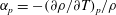 $\unicode[STIX]{x1D6FC}_{p}=-(\unicode[STIX]{x2202}\unicode[STIX]{x1D70C}/\unicode[STIX]{x2202}T)_{p}/\unicode[STIX]{x1D70C}$
, is maximum. A pseudophase transition, or simply pseudotransition, occurs, for example, when temperature changes from
$\unicode[STIX]{x1D6FC}_{p}=-(\unicode[STIX]{x2202}\unicode[STIX]{x1D70C}/\unicode[STIX]{x2202}T)_{p}/\unicode[STIX]{x1D70C}$
, is maximum. A pseudophase transition, or simply pseudotransition, occurs, for example, when temperature changes from
 $T<T_{pb}$
to
$T<T_{pb}$
to
 $T>T_{pb}$
(or vice versa), for given supercritical pressure conditions
$T>T_{pb}$
(or vice versa), for given supercritical pressure conditions
 $p=p_{pb}$
, hence crossing the PBL in the
$p=p_{pb}$
, hence crossing the PBL in the
 $p{-}T$
phase diagram. The goal of the present work is to investigate the dynamics of turbulent heat and mass transfer when the instantaneous temperature and density fields fluctuate about such pseudoboiling conditions, also referred to here as transcritical temperature conditions.
$p{-}T$
phase diagram. The goal of the present work is to investigate the dynamics of turbulent heat and mass transfer when the instantaneous temperature and density fields fluctuate about such pseudoboiling conditions, also referred to here as transcritical temperature conditions.
Unlike a subcritical phase change where the concept of latent heat accounts for the discontinuity of enthalpy, supercritical pseudotransition takes place progressively over a finite temperature range bracketing pseudoboiling conditions. While molecules are homogeneously distributed in space with a well-defined mean free path in the liquid-like (
 $T\ll T_{pb}$
) or gas-like (
$T\ll T_{pb}$
) or gas-like (
 $T\gg T_{pb}$
) supercritical states, heterogeneously distributed microscopic clusters of tightly packed molecules are formed during pseudotransition (Tucker Reference Tucker1999). This results in abrupt changes in compressibility and density, and a rapid, albeit continuous, increase in the heat capacity, with gas-like behaviour retained between denser molecular clusters. This heterogeneous microscopic distribution results in optical dispersion effects allowing the experimental identification of pseudotransition (Gorelli et al.
Reference Gorelli, Santoro, Scopigno, Krisch and Ruocco2006; Simeoni et al.
Reference Simeoni, Bryk, Gorelli, Krisch, Ruocco, Santoro and Scopigno2010).
$T\gg T_{pb}$
) supercritical states, heterogeneously distributed microscopic clusters of tightly packed molecules are formed during pseudotransition (Tucker Reference Tucker1999). This results in abrupt changes in compressibility and density, and a rapid, albeit continuous, increase in the heat capacity, with gas-like behaviour retained between denser molecular clusters. This heterogeneous microscopic distribution results in optical dispersion effects allowing the experimental identification of pseudotransition (Gorelli et al.
Reference Gorelli, Santoro, Scopigno, Krisch and Ruocco2006; Simeoni et al.
Reference Simeoni, Bryk, Gorelli, Krisch, Ruocco, Santoro and Scopigno2010).
Due to the steep variations of macroscopic thermodynamic properties near the PBL, accurate simulations of flows in transcritical temperature conditions are numerically challenging. Also, an Eulerian approach based on the fully compressible conservative Navier–Stokes equations coupled with highly nonlinear equations of state is less robust to inadequate spatial resolution, resulting in spurious numerical oscillations (Kawai, Terashima & Negishi Reference Kawai, Terashima and Negishi2015). To bypass such stability constraints, Terashima, Kawai & Yamanishi (Reference Terashima, Kawai and Yamanishi2011), Terashima & Koshi (Reference Terashima and Koshi2012, Reference Terashima and Koshi2013) and Kawai (Reference Kawai2016) used a non-conservative pressure-based formulation coupled with the use of artificial viscosity, successfully suppressing non-physical oscillations at the expense of energy conservation. Alternative approaches have used a double-flux formulation (Ma, Lv & Ihme Reference Ma, Lv and Ihme2017), inspired by the interfacial flow community, where the flux at one face is computed twice, each time assuming a specific heat ratio taken alternatively from the left or right side of the flux face. Other works, such as Peeters et al. (Reference Peeters, Pecnik, Rohde, van der Hagen and Boersma2016), use a low-Mach-number formulation neglecting compressibility effects such as acoustic wave propagation with significant gains in computational time and stability. In the present study, a fully compressible and conservative approach is adopted, where numerical stability issues are contained via systematic grid refinement in the canonical setting of channel flow turbulence. To ensure numerical stability on coarse grids, the conserved variables are explicitly filtered at every time step.
Transcritical temperature conditions have been found to enhance heat transfer fluctuations and alter turbulence production rates in wall-bounded flows (Yoo Reference Yoo2013). Such deviations from ideal gas behaviour are not to be confused with real fluid effects, which refers to molecularly disassociated gases occurring in hypersonic flows. Real fluid effects in a flat-plate turbulent boundary layer over a heated wall were studied by Kawai (Reference Kawai2016); he found that Morkovin’s hypothesis (Morkovin Reference Morkovin1962) is not applicable to pseudophase changing conditions due to the presence of significant density fluctuations yielding non-classical effects in the mass flux, turbulent diffusion and pressure dilatation distributions. Patel et al. (Reference Patel, Peeters, Boersma and Pecnik2015) numerically and theoretically investigated the near-wall scaling laws in a turbulent channel flow with large thermophysical property variations. They confirmed that the turbulent flow statistics exhibit quasi-similarity based on a semi-local friction Reynolds number,
 $Re_{\unicode[STIX]{x1D70F}}^{\ast }\equiv Re_{\unicode[STIX]{x1D70F}}\sqrt{(\bar{\unicode[STIX]{x1D70C}}/\bar{\unicode[STIX]{x1D70C}}_{w})}/(\bar{\unicode[STIX]{x1D707}}/\bar{\unicode[STIX]{x1D707}}_{w})$
, where the overbar refers to Reynolds averaging and the subscript
$Re_{\unicode[STIX]{x1D70F}}^{\ast }\equiv Re_{\unicode[STIX]{x1D70F}}\sqrt{(\bar{\unicode[STIX]{x1D70C}}/\bar{\unicode[STIX]{x1D70C}}_{w})}/(\bar{\unicode[STIX]{x1D707}}/\bar{\unicode[STIX]{x1D707}}_{w})$
, where the overbar refers to Reynolds averaging and the subscript
 $w$
to the averaged wall quantity. Their investigation was, however, limited to a density ratio of
$w$
to the averaged wall quantity. Their investigation was, however, limited to a density ratio of
 $\bar{\unicode[STIX]{x1D70C}}/\bar{\unicode[STIX]{x1D70C}}_{w}=0.4$
–1.0. From direct numerical simulations (DNS) of dense-gas, supersonic turbulent channel flows by Sciacovelli, Cinnella & Gloerfelt (Reference Sciacovelli, Cinnella and Gloerfelt2017), it was found that the transport properties are dependent on density and temperature of the fluid and the speed of sound varies non-monotonically due to dense gas effects (or real fluid effects in this study). The dense gas effects caused the maximum levels of the fluctuating density root-mean-square to be located in the viscous sublayer, which is different from the ideal gas case locating in the buffer layer, so that the density fluctuations do not change the turbulent structures significantly in the channel and Morkovin’s hypothesis holds. In the present paper, we explore the application of the conventionally scaled van Driest transformation (van Driest Reference van Driest1951), as well as the semi-locally scaled one (Huang, Coleman & Bradshaw Reference Huang, Coleman and Bradshaw1995) in the context of transcritical boundary layers. We also explore the transformation by Trettel & Larsson (Reference Trettel and Larsson2016), which performs comparably to the aforementioned transformations, contrary to that shown by Ma, Yang & Ihme (Reference Ma, Yang and Ihme2018). Nemati et al. (Reference Nemati, Patel, Boersma and Pecnik2015) performed DNS of a heated turbulent pipe flow at supercritical pressure where thermal expansion due to a constant wall heat flux in the presence of low buoyancy effects was found to attenuate turbulent kinetic energy; turbulence enhancement was observed for high buoyancy cases. Pizzarelli et al. (Reference Pizzarelli, Nasuti, Paciorri and Onofri2009) studied turbulent rectangular channel flow at supercritical pressure with high wall heat flux, finding that real fluid effects attenuate heat transfer significantly at the channel corners. Compressible channel flow simulations at supercritical pressures and transcritical temperatures by Sengupta et al. (Reference Sengupta, Nemati, Boersma and Pecnik2017) show that the cold wall region has higher density and temperature fluctuations as well as higher coherence than the hot near-wall region. Also, the liquid-like flow region is characterized by decreased streamwise and increased spanwise anisotropy and vice versa in the region of gas-like behaviour.
$\bar{\unicode[STIX]{x1D70C}}/\bar{\unicode[STIX]{x1D70C}}_{w}=0.4$
–1.0. From direct numerical simulations (DNS) of dense-gas, supersonic turbulent channel flows by Sciacovelli, Cinnella & Gloerfelt (Reference Sciacovelli, Cinnella and Gloerfelt2017), it was found that the transport properties are dependent on density and temperature of the fluid and the speed of sound varies non-monotonically due to dense gas effects (or real fluid effects in this study). The dense gas effects caused the maximum levels of the fluctuating density root-mean-square to be located in the viscous sublayer, which is different from the ideal gas case locating in the buffer layer, so that the density fluctuations do not change the turbulent structures significantly in the channel and Morkovin’s hypothesis holds. In the present paper, we explore the application of the conventionally scaled van Driest transformation (van Driest Reference van Driest1951), as well as the semi-locally scaled one (Huang, Coleman & Bradshaw Reference Huang, Coleman and Bradshaw1995) in the context of transcritical boundary layers. We also explore the transformation by Trettel & Larsson (Reference Trettel and Larsson2016), which performs comparably to the aforementioned transformations, contrary to that shown by Ma, Yang & Ihme (Reference Ma, Yang and Ihme2018). Nemati et al. (Reference Nemati, Patel, Boersma and Pecnik2015) performed DNS of a heated turbulent pipe flow at supercritical pressure where thermal expansion due to a constant wall heat flux in the presence of low buoyancy effects was found to attenuate turbulent kinetic energy; turbulence enhancement was observed for high buoyancy cases. Pizzarelli et al. (Reference Pizzarelli, Nasuti, Paciorri and Onofri2009) studied turbulent rectangular channel flow at supercritical pressure with high wall heat flux, finding that real fluid effects attenuate heat transfer significantly at the channel corners. Compressible channel flow simulations at supercritical pressures and transcritical temperatures by Sengupta et al. (Reference Sengupta, Nemati, Boersma and Pecnik2017) show that the cold wall region has higher density and temperature fluctuations as well as higher coherence than the hot near-wall region. Also, the liquid-like flow region is characterized by decreased streamwise and increased spanwise anisotropy and vice versa in the region of gas-like behaviour.
In the present paper, we analyse data from DNS of compressible channel flow turbulence maintained in pseudophase changing conditions by a wall-to-wall temperature difference imposed via isothermal conditions. The dataset presented here has been considerably expanded with respect to previous publications by the authors (Kim, Hickey & Scalo Reference Kim, Hickey and Scalo2017a ; Kim, Scalo & Hickey Reference Kim, Scalo and Hickey2017b ) and analysed in more depth. In the following, we first describe the governing equations, the fluid model and the computational set-up (§ 2). The mean and fluctuating hydrodynamic and thermodynamic quantities are then presented together with probability distribution functions (p.d.f.s) (§§ 3 and 4). Finally, instantaneous turbulent structures are investigated and compared with the correlation statistics to infer their role in the heat- and mass-transfer dynamics focusing on the near-wall region (§ 5).
2 Problem formulation
2.1 Governing equations
The governing equations of mass, momentum and total energy for a fully compressible flow are solved in conservative form which reads
 $$\begin{eqnarray}\displaystyle & \displaystyle \frac{\unicode[STIX]{x2202}\unicode[STIX]{x1D70C}}{\unicode[STIX]{x2202}t}+\frac{\unicode[STIX]{x2202}\unicode[STIX]{x1D70C}u_{j}}{\unicode[STIX]{x2202}x_{j}}=0, & \displaystyle\end{eqnarray}$$
 $$\begin{eqnarray}\displaystyle & \displaystyle \frac{\unicode[STIX]{x2202}\unicode[STIX]{x1D70C}u_{i}}{\unicode[STIX]{x2202}t}+\frac{\unicode[STIX]{x2202}\unicode[STIX]{x1D70C}u_{i}u_{j}}{\unicode[STIX]{x2202}x_{j}}=-\frac{\unicode[STIX]{x2202}p}{\unicode[STIX]{x2202}x_{j}}+\frac{\unicode[STIX]{x2202}\unicode[STIX]{x1D70F}_{ij}}{\unicode[STIX]{x2202}x_{j}}, & \displaystyle\end{eqnarray}$$
 $$\begin{eqnarray}\displaystyle & \displaystyle \frac{\unicode[STIX]{x2202}\unicode[STIX]{x1D70C}E}{\unicode[STIX]{x2202}t}+\frac{\unicode[STIX]{x2202}}{\unicode[STIX]{x2202}x_{j}}[u_{j}(\unicode[STIX]{x1D70C}E+p)]=\frac{\unicode[STIX]{x2202}}{\unicode[STIX]{x2202}x_{j}}(u_{i}\unicode[STIX]{x1D70F}_{ij}-q_{j}), & \displaystyle\end{eqnarray}$$
 $x_{1}$
,
$x_{1}$
,
 $x_{2}$
and
$x_{2}$
and
 $x_{3}$
(equivalently,
$x_{3}$
(equivalently,
 $x$
,
$x$
,
 $y$
and
$y$
and
 $z$
) are the streamwise, wall-normal and spanwise coordinates, respectively, and
$z$
) are the streamwise, wall-normal and spanwise coordinates, respectively, and
 $u_{i}$
is the velocity component in the
$u_{i}$
is the velocity component in the
 $i$
th direction,
$i$
th direction,
 $t$
the time,
$t$
the time,
 $\unicode[STIX]{x1D70C}$
the density,
$\unicode[STIX]{x1D70C}$
the density,
 $p$
the pressure and
$p$
the pressure and
 $E$
the total energy per unit mass. Unless otherwise stated, all the symbols refer to dimensional quantities.
$E$
the total energy per unit mass. Unless otherwise stated, all the symbols refer to dimensional quantities.The viscous and conductive heat fluxes in (2.1b ) and (2.1c ) are, respectively,
 $$\begin{eqnarray}\displaystyle & \displaystyle \unicode[STIX]{x1D70F}_{ij}=2\unicode[STIX]{x1D707}\left[\unicode[STIX]{x1D61A}_{ij}-\frac{1}{3}\frac{\unicode[STIX]{x2202}u_{k}}{\unicode[STIX]{x2202}x_{k}}\unicode[STIX]{x1D6FF}_{ij}\right], & \displaystyle\end{eqnarray}$$
 $$\begin{eqnarray}\displaystyle & \displaystyle q_{j}=-\unicode[STIX]{x1D706}\frac{\unicode[STIX]{x2202}T}{\unicode[STIX]{x2202}x_{j}}=-\frac{c_{p}\unicode[STIX]{x1D707}}{Pr}\frac{\unicode[STIX]{x2202}T}{\unicode[STIX]{x2202}x_{j}}, & \displaystyle\end{eqnarray}$$
 $\unicode[STIX]{x1D707}$
is the dynamic viscosity,
$\unicode[STIX]{x1D707}$
is the dynamic viscosity,
 $\unicode[STIX]{x1D61A}_{ij}$
the strain rate tensor given by
$\unicode[STIX]{x1D61A}_{ij}$
the strain rate tensor given by
 $\unicode[STIX]{x1D61A}_{ij}=(\unicode[STIX]{x2202}u_{j}/\unicode[STIX]{x2202}x_{i}+\unicode[STIX]{x2202}u_{i}/\unicode[STIX]{x2202}x_{j})/2$
,
$\unicode[STIX]{x1D61A}_{ij}=(\unicode[STIX]{x2202}u_{j}/\unicode[STIX]{x2202}x_{i}+\unicode[STIX]{x2202}u_{i}/\unicode[STIX]{x2202}x_{j})/2$
,
 $\unicode[STIX]{x1D706}$
the thermal conductivity,
$\unicode[STIX]{x1D706}$
the thermal conductivity,
 $c_{p}$
the heat capacity at constant pressure,
$c_{p}$
the heat capacity at constant pressure,
 $Pr$
the Prandtl number and
$Pr$
the Prandtl number and
 $T$
the temperature.
$T$
the temperature.2.2 Real fluid model
The Peng–Robinson (PR) equation of state (EoS) (Peng & Robinson Reference Peng and Robinson1976) is used to model the working fluid of choice for this study, R-134a (1,1,1,2-tetrafluoroethane,
 $\text{CH}_{2}\text{FCF}_{3}$
), which benefits from experimentally accessible critical pressures and temperatures of
$\text{CH}_{2}\text{FCF}_{3}$
), which benefits from experimentally accessible critical pressures and temperatures of
 $p_{cr}=40.59$
bar and
$p_{cr}=40.59$
bar and
 $T_{cr}=374.26$
K and is widely used in turbomachinery and heat exchangers as a cooling fluid because of its non-toxic and non-flammable characteristics. Departure functions guaranteeing full thermodynamic consistency with the chosen EoS have been derived following Ewing & Peters (Reference Ewing and Peters2000). Transport properties such as the dynamic viscosity and thermal conductivity are estimated via Chung’s method (Chung et al.
Reference Chung, Ajlan, Lee and Starling1988) which predicts experimental values within 5 % error (Poling, Prausnitz & O’Connell Reference Poling, Prausnitz and O’Connell2001). The choice of an accurate and simple EoS such as the PR EoS provides a consistent thermodynamic model, computationally less expensive than interpolating tabulated values. In order to prove adequacy and accuracy of implementation of the equations, detailed derivations and comparisons against the NIST database (Lemmon, McLinden & Friend Reference Lemmon, McLinden and Friend2016) (figure 27) are included in appendix A.
$T_{cr}=374.26$
K and is widely used in turbomachinery and heat exchangers as a cooling fluid because of its non-toxic and non-flammable characteristics. Departure functions guaranteeing full thermodynamic consistency with the chosen EoS have been derived following Ewing & Peters (Reference Ewing and Peters2000). Transport properties such as the dynamic viscosity and thermal conductivity are estimated via Chung’s method (Chung et al.
Reference Chung, Ajlan, Lee and Starling1988) which predicts experimental values within 5 % error (Poling, Prausnitz & O’Connell Reference Poling, Prausnitz and O’Connell2001). The choice of an accurate and simple EoS such as the PR EoS provides a consistent thermodynamic model, computationally less expensive than interpolating tabulated values. In order to prove adequacy and accuracy of implementation of the equations, detailed derivations and comparisons against the NIST database (Lemmon, McLinden & Friend Reference Lemmon, McLinden and Friend2016) (figure 27) are included in appendix A.
2.3 Computational set-up
The proposed numerical simulations have been carried out with Hybrid, a fully compressible Navier–Stokes solver originally written by Johan Larsson. This code utilizes a finite central difference scheme with a fourth-order accuracy by summation-by-parts operators for the inviscid terms and a second-order accuracy for the viscous terms. The time advancement is achieved by a fourth-order-accurate Runge–Kutta method. Hybrid has been used in several canonical numerical investigations such as those involving shock–vortex interaction, compressible homogeneous isotropic turbulence (Larsson, Lele & Moin Reference Larsson, Lele and Moin2007) and shock–turbulence interaction (Larsson & Lele Reference Larsson and Lele2009; Larsson, Bermejo-Moreno & Lele Reference Larsson, Bermejo-Moreno and Lele2013). The code solves single-component fluid, which is a suitable modelling approach for a supercritical pressure flow since surface tension becomes negligible for supercritical pressures,
 $p>p_{cr}$
, and numerical techniques for multiphase simulations such as interface tracking or reconstruction are not required. New features that have been added to the code include parallel HDF5 (The HDF Group 1998) input/output capabilities and a generic EoS.
$p>p_{cr}$
, and numerical techniques for multiphase simulations such as interface tracking or reconstruction are not required. New features that have been added to the code include parallel HDF5 (The HDF Group 1998) input/output capabilities and a generic EoS.
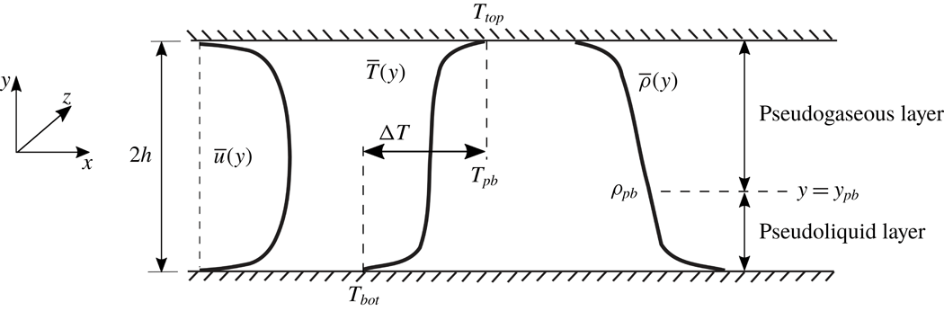
The computational setup is a compressible turbulent channel flow (figure 2) kept at a nominal bulk pressure of
 $p_{b}\simeq 1.1p_{cr}$
corresponding to a pseudoboiling temperature of
$p_{b}\simeq 1.1p_{cr}$
corresponding to a pseudoboiling temperature of
 $T_{pb}=379.1$
K defined based on the maximum isobaric thermal expansion coefficient,
$T_{pb}=379.1$
K defined based on the maximum isobaric thermal expansion coefficient,
 $\unicode[STIX]{x1D6FC}_{p}=-(\unicode[STIX]{x2202}\unicode[STIX]{x1D70C}/\unicode[STIX]{x2202}T)_{p}/\unicode[STIX]{x1D70C}$
(figure 1
a). The assigned isothermal top- and bottom-wall boundary conditions bracket the pseudoboiling temperature (
$\unicode[STIX]{x1D6FC}_{p}=-(\unicode[STIX]{x2202}\unicode[STIX]{x1D70C}/\unicode[STIX]{x2202}T)_{p}/\unicode[STIX]{x1D70C}$
(figure 1
a). The assigned isothermal top- and bottom-wall boundary conditions bracket the pseudoboiling temperature (
 $T_{top/bot}=T_{pb}\pm \unicode[STIX]{x0394}T/2$
) maintaining transcritical temperature conditions (figure1
b).
$T_{top/bot}=T_{pb}\pm \unicode[STIX]{x0394}T/2$
) maintaining transcritical temperature conditions (figure1
b).

Figure 1. Phase diagram for R-134a showing the critical point (
 $p_{cr}=40.59$
bar,
$p_{cr}=40.59$
bar,
 $T_{cr}=374.26$
K) (▫), the PBL (- - -) and the isolines of isobaric thermal expansion coefficient,
$T_{cr}=374.26$
K) (▫), the PBL (- - -) and the isolines of isobaric thermal expansion coefficient,
 $\unicode[STIX]{x1D6FC}_{p}$
(——,
$\unicode[STIX]{x1D6FC}_{p}$
(——,
 $\text{K}^{-1}$
) (a). Density and isobaric heat capacity versus temperature for
$\text{K}^{-1}$
) (a). Density and isobaric heat capacity versus temperature for
 $p=1.1p_{cr}$
with the pseudoboiling point (●) and top-to-bottom temperature differences,
$p=1.1p_{cr}$
with the pseudoboiling point (●) and top-to-bottom temperature differences,
 $\unicode[STIX]{x0394}T$
, bracketing
$\unicode[STIX]{x0394}T$
, bracketing
 $T_{pb}=379.1$
K (b).
$T_{pb}=379.1$
K (b).
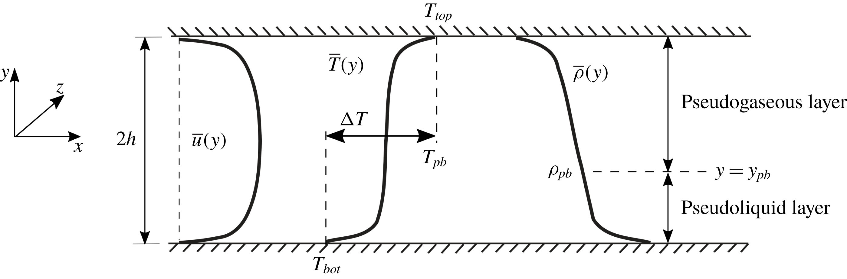
Table 1. Simulation parameters achieving transcritical temperature conditions for R-134a. Bulk parameters are indicated with a subscript ‘
 $b$
’, while pseudoboiling or pseudo(phase)transitioning are indicated with ‘
$b$
’, while pseudoboiling or pseudo(phase)transitioning are indicated with ‘
 $pb$
’.
$pb$
’.

Top- to bottom-wall temperature differences investigated are
 $\unicode[STIX]{x0394}T=T_{top}-T_{bot}=5$
, 10 and 20 K, with bulk density set to
$\unicode[STIX]{x0394}T=T_{top}-T_{bot}=5$
, 10 and 20 K, with bulk density set to
 $\unicode[STIX]{x1D70C}_{b}=450$
,
$\unicode[STIX]{x1D70C}_{b}=450$
,
 $474$
and
$474$
and
 $520~\text{kg}~\text{m}^{-3}$
, respectively, determined via trial and error to obtain the desired bulk pressure for all cases (see tables 1 and 2). Periodic boundary conditions are applied to the streamwise and spanwise directions and the grid is stretched in the wall-normal direction with a hyperbolic tangent law. To guarantee feasibility of the simulations on the finest grid and the highest temperature difference considered where the time step is acoustically limited to
$520~\text{kg}~\text{m}^{-3}$
, respectively, determined via trial and error to obtain the desired bulk pressure for all cases (see tables 1 and 2). Periodic boundary conditions are applied to the streamwise and spanwise directions and the grid is stretched in the wall-normal direction with a hyperbolic tangent law. To guarantee feasibility of the simulations on the finest grid and the highest temperature difference considered where the time step is acoustically limited to
 $\unicode[STIX]{x0394}t=1.4\times 10^{-8}$
, the bulk velocity has been set for all cases to the relatively high value (for typical heat transfer applications) of
$\unicode[STIX]{x0394}t=1.4\times 10^{-8}$
, the bulk velocity has been set for all cases to the relatively high value (for typical heat transfer applications) of
 $U_{b}=36~\text{m}~\text{s}^{-1}$
corresponding to a Mach number in the low-subsonic range of
$U_{b}=36~\text{m}~\text{s}^{-1}$
corresponding to a Mach number in the low-subsonic range of
 $M_{b}=0.26$
with a range of turbulent Mach number
$M_{b}=0.26$
with a range of turbulent Mach number
 $M_{t}=0.015$
(centre region) to 0.051 (near-wall peak). Given the large density variation near the pseudocritical point, buoyancy effects may be important in the mean as well as in the turbulent quantities. In this study, however, the buoyancy effects are neglected in order to focus on structural changes in compressible channel flow turbulence due to wall heat transfer in the presence of real fluid effects.
$M_{t}=0.015$
(centre region) to 0.051 (near-wall peak). Given the large density variation near the pseudocritical point, buoyancy effects may be important in the mean as well as in the turbulent quantities. In this study, however, the buoyancy effects are neglected in order to focus on structural changes in compressible channel flow turbulence due to wall heat transfer in the presence of real fluid effects.
Table 2. Friction Reynolds number and grid resolution in wall units
 $(u_{\unicode[STIX]{x1D70F}}/\unicode[STIX]{x1D708})^{-1}$
for the bottom and top portion of the channel evaluated with respective wall quantities. See also table 1.
$(u_{\unicode[STIX]{x1D70F}}/\unicode[STIX]{x1D708})^{-1}$
for the bottom and top portion of the channel evaluated with respective wall quantities. See also table 1.

To assess the sensitivity of the flow to the thermodynamic gradients near the critical point, a reference simulation at twice the critical pressure (
 $p_{b}=2p_{cr}$
) is carried out with the same working fluid (R-134a) and simulation parameters below. Given the higher pressure, the gradients at the pseudoboiling point are much weaker compared to the near-critical conditions
$p_{b}=2p_{cr}$
) is carried out with the same working fluid (R-134a) and simulation parameters below. Given the higher pressure, the gradients at the pseudoboiling point are much weaker compared to the near-critical conditions
 $p_{b}=1.1p_{cr}$
chosen for the rest of the runs (see comparison in figure 27 in appendix A). It should be noted that some real fluid effects are still present in the higher-pressure case; the thermophysical and thermodynamic variations as a function of temperature are in fact still present, albeit much weaker. For example, for the same
$p_{b}=1.1p_{cr}$
chosen for the rest of the runs (see comparison in figure 27 in appendix A). It should be noted that some real fluid effects are still present in the higher-pressure case; the thermophysical and thermodynamic variations as a function of temperature are in fact still present, albeit much weaker. For example, for the same
 $\unicode[STIX]{x0394}T=20$
K, the relative density difference between the top and bottom walls is only 25 % at
$\unicode[STIX]{x0394}T=20$
K, the relative density difference between the top and bottom walls is only 25 % at
 $p_{b}=2p_{cr}$
; it is 62 % at
$p_{b}=2p_{cr}$
; it is 62 % at
 $p_{b}=1.1p_{cr}$
(see table 3). The parameters of this reference simulation are
$p_{b}=1.1p_{cr}$
(see table 3). The parameters of this reference simulation are
 $\unicode[STIX]{x1D70C}_{b}=596~\text{kg}~\text{m}^{-3}$
,
$\unicode[STIX]{x1D70C}_{b}=596~\text{kg}~\text{m}^{-3}$
,
 $p_{b}=2p_{cr}=81.18$
bar,
$p_{b}=2p_{cr}=81.18$
bar,
 $\unicode[STIX]{x0394}T=20$
K (
$\unicode[STIX]{x0394}T=20$
K (
 $T_{bot}=394.9$
K and
$T_{bot}=394.9$
K and
 $T_{top}=414.9$
K where the pseudoboiling temperature is
$T_{top}=414.9$
K where the pseudoboiling temperature is
 $T_{pb}=404.9$
K at the given pressure) and
$T_{pb}=404.9$
K at the given pressure) and
 $U_{b}=36~\text{m}~\text{s}^{-1}$
.
$U_{b}=36~\text{m}~\text{s}^{-1}$
.
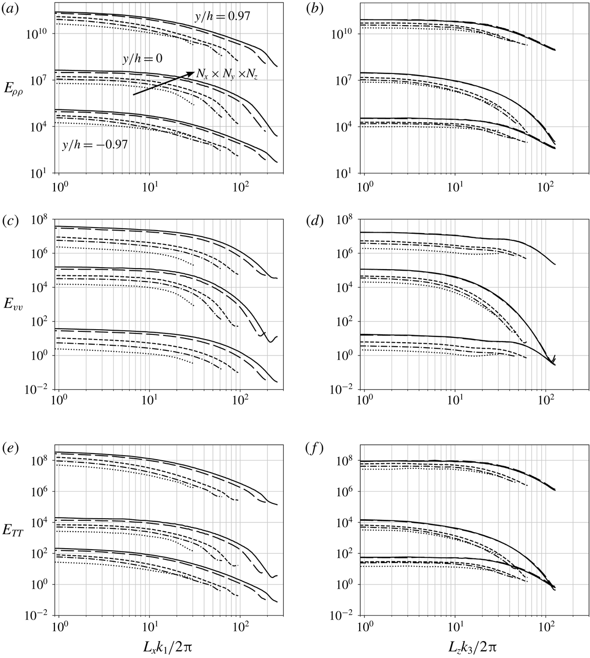
To ensure the proper spatial resolution of all relevant hydrodynamic and thermodynamic scales, a systematic grid refinement study has been carried out (see appendix B and table 2); this is especially important in simulations of supercritical flows in the near-critical or pseudophase transitioning conditions (see Introduction). The relevant metric of the spectral broadening level for channel flow turbulence is the friction Reynolds number,
 $$\begin{eqnarray}\displaystyle Re_{\unicode[STIX]{x1D70F}}=\frac{u_{\unicode[STIX]{x1D70F}}h}{\unicode[STIX]{x1D708}_{w}}, & & \displaystyle\end{eqnarray}$$
based on the friction velocity,
 $u_{\unicode[STIX]{x1D70F}}$
, the channel half-height,
$u_{\unicode[STIX]{x1D70F}}$
, the channel half-height,
 $h$
, and the kinematic viscosity at the wall,
$h$
, and the kinematic viscosity at the wall,
 $\unicode[STIX]{x1D708}_{w}$
, of the fluid. It can be viewed as the channel half-height normalized by the viscous length scale,
$\unicode[STIX]{x1D708}_{w}$
, of the fluid. It can be viewed as the channel half-height normalized by the viscous length scale,
 $\unicode[STIX]{x1D708}_{w}/u_{\unicode[STIX]{x1D70F}}=\unicode[STIX]{x1D708}_{w}/(\unicode[STIX]{x2202}u/\unicode[STIX]{x2202}x_{2})_{x_{2}=0}$
, hence
$\unicode[STIX]{x1D708}_{w}/u_{\unicode[STIX]{x1D70F}}=\unicode[STIX]{x1D708}_{w}/(\unicode[STIX]{x2202}u/\unicode[STIX]{x2202}x_{2})_{x_{2}=0}$
, hence
 $Re_{\unicode[STIX]{x1D70F}}=h^{+}$
. Therefore,
$Re_{\unicode[STIX]{x1D70F}}=h^{+}$
. Therefore,
 $Re_{\unicode[STIX]{x1D70F}}$
is the ratio of an integral length scale,
$Re_{\unicode[STIX]{x1D70F}}$
is the ratio of an integral length scale,
 ${\sim}h$
, to a viscous scale evaluated at the wall. Typical practice in DNS is to adopt relatively low values of friction Reynolds number to enable full resolution of the relevant scales. For the present simulations, this is achieved by augmenting dynamic viscosity and thermal conductivity by the same multiplicative factor (figure 3) resulting in
${\sim}h$
, to a viscous scale evaluated at the wall. Typical practice in DNS is to adopt relatively low values of friction Reynolds number to enable full resolution of the relevant scales. For the present simulations, this is achieved by augmenting dynamic viscosity and thermal conductivity by the same multiplicative factor (figure 3) resulting in
 $Re_{\unicode[STIX]{x1D70F}}$
in the range of 342–394 (table 2). This choice leaves the Prandtl number unaltered and reproduces the correct trend of transport properties in the transcritical regime (see appendix A). The reference simulation has been carried out at
$Re_{\unicode[STIX]{x1D70F}}$
in the range of 342–394 (table 2). This choice leaves the Prandtl number unaltered and reproduces the correct trend of transport properties in the transcritical regime (see appendix A). The reference simulation has been carried out at
 $Re_{\unicode[STIX]{x1D70F}}=366$
,
$Re_{\unicode[STIX]{x1D70F}}=366$
,
 $\unicode[STIX]{x0394}x^{+}=10.98$
,
$\unicode[STIX]{x0394}x^{+}=10.98$
,
 $\unicode[STIX]{x0394}y^{+}=0.43$
–5.93,
$\unicode[STIX]{x0394}y^{+}=0.43$
–5.93,
 $\unicode[STIX]{x0394}z^{+}=5.63$
for the bottom wall and
$\unicode[STIX]{x0394}z^{+}=5.63$
for the bottom wall and
 $Re_{\unicode[STIX]{x1D70F}}=386$
,
$Re_{\unicode[STIX]{x1D70F}}=386$
,
 $\unicode[STIX]{x0394}x^{+}=11.58$
,
$\unicode[STIX]{x0394}x^{+}=11.58$
,
 $\unicode[STIX]{x0394}y^{+}=0.46$
–6.25,
$\unicode[STIX]{x0394}y^{+}=0.46$
–6.25,
 $\unicode[STIX]{x0394}z^{+}=5.94$
for the top wall.
$\unicode[STIX]{x0394}z^{+}=5.94$
for the top wall.

Figure 3. Dynamic viscosity
 $\unicode[STIX]{x1D707}$
, thermal conductivity
$\unicode[STIX]{x1D707}$
, thermal conductivity
 $\unicode[STIX]{x1D706}$
and Prandtl number
$\unicode[STIX]{x1D706}$
and Prandtl number
 $Pr$
for R-134a taken from Chung’s model (——) (see appendix A); scaled dynamic viscosity and conductivity (- - -), augmented by a factor of 60, used in the computations, yielding the same Prandtl number.
$Pr$
for R-134a taken from Chung’s model (——) (see appendix A); scaled dynamic viscosity and conductivity (- - -), augmented by a factor of 60, used in the computations, yielding the same Prandtl number.
Table 3. Top- and bottom-wall values of mean density and compressibility factor and average location of pseudophase transition
 $y_{pb}$
for various temperature conditions. With the exception of
$y_{pb}$
for various temperature conditions. With the exception of
 $\unicode[STIX]{x0394}T$
, all values reported are a result of the calculations. The first three rows are related to the
$\unicode[STIX]{x0394}T$
, all values reported are a result of the calculations. The first three rows are related to the
 $p_{b}=1.1p_{cr}$
cases, the last row to the reference high-pressure case
$p_{b}=1.1p_{cr}$
cases, the last row to the reference high-pressure case
 $p_{b}=2p_{cr}$
.
$p_{b}=2p_{cr}$
.

3 First- and second-order statistics
In this section, a statistical analysis limited to the first- and second-order moments of turbulent fluctuations in the transcritical channel flow set-up of figure 2 is carried out in comparison with a reference simulation at
 $p_{b}=2p_{cr}$
, exhibiting very mild thermodynamic gradients at the pseudoboiling point (see comparison in figure 27 in appendix A).
$p_{b}=2p_{cr}$
, exhibiting very mild thermodynamic gradients at the pseudoboiling point (see comparison in figure 27 in appendix A).
3.1 Mean flow quantities

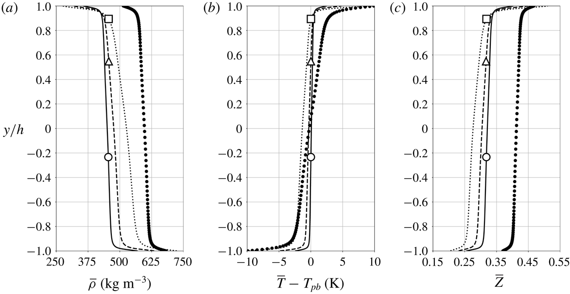
Figure 4. Reynolds-averaged density (a), temperature (b) and compressibility factor (c) for
 $p_{b}=1.1p_{cr}$
and
$p_{b}=1.1p_{cr}$
and
 $\unicode[STIX]{x0394}T=5$
K (——), 10 K (- - -) and 20 K (
$\unicode[STIX]{x0394}T=5$
K (——), 10 K (- - -) and 20 K (
 $\cdots \cdots$
) and reference data for
$\cdots \cdots$
) and reference data for
 $p_{b}=2p_{cr}$
and
$p_{b}=2p_{cr}$
and
 $\unicode[STIX]{x0394}T=20$
K (●) (see § 2.3). Average location of pseudotransition for
$\unicode[STIX]{x0394}T=20$
K (●) (see § 2.3). Average location of pseudotransition for
 $\unicode[STIX]{x0394}T=5~\text{K}$
(○), 10 K (▵) and 20 K (▫).
$\unicode[STIX]{x0394}T=5~\text{K}$
(○), 10 K (▵) and 20 K (▫).
Figure 4 shows Reynolds-averaged profiles of density, temperature and compressibility factor
 $Z=p/(\unicode[STIX]{x1D70C}R_{gas}T)$
, where
$Z=p/(\unicode[STIX]{x1D70C}R_{gas}T)$
, where
 $R_{gas}=81.49~\text{J}~\text{kg}^{-1}~\text{K}^{-1}$
is the gas constant for R-134a. The top-to-bottom density difference (table 3) of
$R_{gas}=81.49~\text{J}~\text{kg}^{-1}~\text{K}^{-1}$
is the gas constant for R-134a. The top-to-bottom density difference (table 3) of
 $\unicode[STIX]{x0394}\unicode[STIX]{x1D70C}=447.5~\text{kg}~\text{m}^{-3}$
achieved under transcritical conditions at
$\unicode[STIX]{x0394}\unicode[STIX]{x1D70C}=447.5~\text{kg}~\text{m}^{-3}$
achieved under transcritical conditions at
 $1.1p_{cr}$
for
$1.1p_{cr}$
for
 $\unicode[STIX]{x0394}T=20~\text{K}$
is about 2.67 times higher than
$\unicode[STIX]{x0394}T=20~\text{K}$
is about 2.67 times higher than
 $\unicode[STIX]{x0394}\unicode[STIX]{x1D70C}=167.4~\text{kg}~\text{m}^{-3}$
, obtained at twice the critical pressure for the same
$\unicode[STIX]{x0394}\unicode[STIX]{x1D70C}=167.4~\text{kg}~\text{m}^{-3}$
, obtained at twice the critical pressure for the same
 $\unicode[STIX]{x0394}T$
. Remarkably, as shown later, density fluctuation intensities for
$\unicode[STIX]{x0394}T$
. Remarkably, as shown later, density fluctuation intensities for
 $\unicode[STIX]{x0394}T=20$
K and
$\unicode[STIX]{x0394}T=20$
K and
 $2p_{cr}$
are very similar to those observed for
$2p_{cr}$
are very similar to those observed for
 $\unicode[STIX]{x0394}T=5$
K and
$\unicode[STIX]{x0394}T=5$
K and
 $1.1p_{cr}$
; in the latter case, however, higher temperature fluctuations are obtained. As expected for higher pressure conditions (see figure 27), a gradual change is also observed in the compressibility factor for the reference data analogous to the density.
$1.1p_{cr}$
; in the latter case, however, higher temperature fluctuations are obtained. As expected for higher pressure conditions (see figure 27), a gradual change is also observed in the compressibility factor for the reference data analogous to the density.
As
 $\unicode[STIX]{x0394}T$
is increased, the average location of pseudotransition
$\unicode[STIX]{x0394}T$
is increased, the average location of pseudotransition
 $y_{pb}$
, where the real fluid effects are expected to be the most accentuated, moves from a near-centreplane location to the upper wall. The same holds when keeping
$y_{pb}$
, where the real fluid effects are expected to be the most accentuated, moves from a near-centreplane location to the upper wall. The same holds when keeping
 $\unicode[STIX]{x0394}T$
constant and lowering the base pressure. It is important to recall that the isothermal wall conditions are selected to be exactly
$\unicode[STIX]{x0394}T$
constant and lowering the base pressure. It is important to recall that the isothermal wall conditions are selected to be exactly
 $\unicode[STIX]{x0394}T/2$
warmer (top) and colder (bottom) than the pseudoboiling temperature; yet the location of the pseudotransition in the channel is not located at the centreplane and it is an output of the calculation. The shift of the pseudotransition location is related to the highly nonlinear and asymmetric thermophysical properties of the fluid about the pseudoboiling point, especially the specific heat capacity. In the transcritical regime, the pseudophase change is accompanied by a finite peak in the specific heat capacity which acts as a thermal barrier. We make an approximation that the enthalpy difference from the cold wall to the pseudoboiling point,
$\unicode[STIX]{x0394}T/2$
warmer (top) and colder (bottom) than the pseudoboiling temperature; yet the location of the pseudotransition in the channel is not located at the centreplane and it is an output of the calculation. The shift of the pseudotransition location is related to the highly nonlinear and asymmetric thermophysical properties of the fluid about the pseudoboiling point, especially the specific heat capacity. In the transcritical regime, the pseudophase change is accompanied by a finite peak in the specific heat capacity which acts as a thermal barrier. We make an approximation that the enthalpy difference from the cold wall to the pseudoboiling point,
 $\unicode[STIX]{x0394}h_{pl}$
(pseudoliquid), is approximately equal to the enthalpy difference from the pseudoboiling point to the warm wall,
$\unicode[STIX]{x0394}h_{pl}$
(pseudoliquid), is approximately equal to the enthalpy difference from the pseudoboiling point to the warm wall,
 $\unicode[STIX]{x0394}h_{pg}$
(pseudogas). In other words, we assume:
$\unicode[STIX]{x0394}h_{pg}$
(pseudogas). In other words, we assume:
 $\unicode[STIX]{x0394}h_{pl}\approx \unicode[STIX]{x0394}h_{pg}$
. Given the small temperature difference between both walls, the error of this approximation is between 3.5 % (for the
$\unicode[STIX]{x0394}h_{pl}\approx \unicode[STIX]{x0394}h_{pg}$
. Given the small temperature difference between both walls, the error of this approximation is between 3.5 % (for the
 $\unicode[STIX]{x0394}5~\text{K}$
case) and 4.6 % (for the
$\unicode[STIX]{x0394}5~\text{K}$
case) and 4.6 % (for the
 $\unicode[STIX]{x0394}20~\text{K}$
case) based on the NIST data. Using this simplifying assumption, we can relate the total enthalpy of the pseudogas and pseudoliquid domain of the flow by the following relationship:
$\unicode[STIX]{x0394}20~\text{K}$
case) based on the NIST data. Using this simplifying assumption, we can relate the total enthalpy of the pseudogas and pseudoliquid domain of the flow by the following relationship:
 $$\begin{eqnarray}\displaystyle {\mathcal{V}}_{pg}\int _{T_{pb}-\unicode[STIX]{x0394}T/2}^{T_{pb}}\unicode[STIX]{x1D70C}c_{p}\,\text{d}T={\mathcal{V}}_{pl}\int _{T_{pb}}^{T_{pb}+\unicode[STIX]{x0394}T/2}\unicode[STIX]{x1D70C}c_{p}\,\text{d}T, & & \displaystyle\end{eqnarray}$$
where the terms
 ${\mathcal{V}}_{pg}$
and
${\mathcal{V}}_{pg}$
and
 ${\mathcal{V}}_{pl}$
respectively denote the volume of the pseudogas and pseudoliquid phases. By computing this relation based on the tabulated properties, we can estimate the relative volume of pseudogas and pseudoliquid in the simulation. It is clear that under perfect gas conditions and/or modest density variation (e.g. away from the critical point), the volume of fluid below and above the average temperature would be equal. In fact, our reference simulation at
${\mathcal{V}}_{pl}$
respectively denote the volume of the pseudogas and pseudoliquid phases. By computing this relation based on the tabulated properties, we can estimate the relative volume of pseudogas and pseudoliquid in the simulation. It is clear that under perfect gas conditions and/or modest density variation (e.g. away from the critical point), the volume of fluid below and above the average temperature would be equal. In fact, our reference simulation at
 $p_{b}=2p_{cr}$
, which shows a very modest variation in thermophysical properties compared to the other runs at
$p_{b}=2p_{cr}$
, which shows a very modest variation in thermophysical properties compared to the other runs at
 $p_{b}=1.1p_{cr}$
, contains about 55 % volume of pseudoliquid based on the above relation. This compares favourably to the simulation results which show the pseudotransition point at the middle of the domain (figure 4
b). When considering the cases at
$p_{b}=1.1p_{cr}$
, contains about 55 % volume of pseudoliquid based on the above relation. This compares favourably to the simulation results which show the pseudotransition point at the middle of the domain (figure 4
b). When considering the cases at
 $p_{b}\approx 1.1p_{cr}$
, we find the pseudoliquid volume takes up 37.0 %, 69.6 % and 76.1 % for the
$p_{b}\approx 1.1p_{cr}$
, we find the pseudoliquid volume takes up 37.0 %, 69.6 % and 76.1 % for the
 $\unicode[STIX]{x0394}T=5$
, 10 and 20 K cases, respectively, based on this simple model. This trend corresponds favourably to the average pseudotransition height computed from the DNS which is 38.5 %, 77.5 % and 94.5 %. These results support the idea that high nonlinearity of the thermophysics near the critical point will dictate the location of the pseudoboiling point relative to the solid walls. As shown here, this is in fact a first-order real fluid effect.
$\unicode[STIX]{x0394}T=5$
, 10 and 20 K cases, respectively, based on this simple model. This trend corresponds favourably to the average pseudotransition height computed from the DNS which is 38.5 %, 77.5 % and 94.5 %. These results support the idea that high nonlinearity of the thermophysics near the critical point will dictate the location of the pseudoboiling point relative to the solid walls. As shown here, this is in fact a first-order real fluid effect.
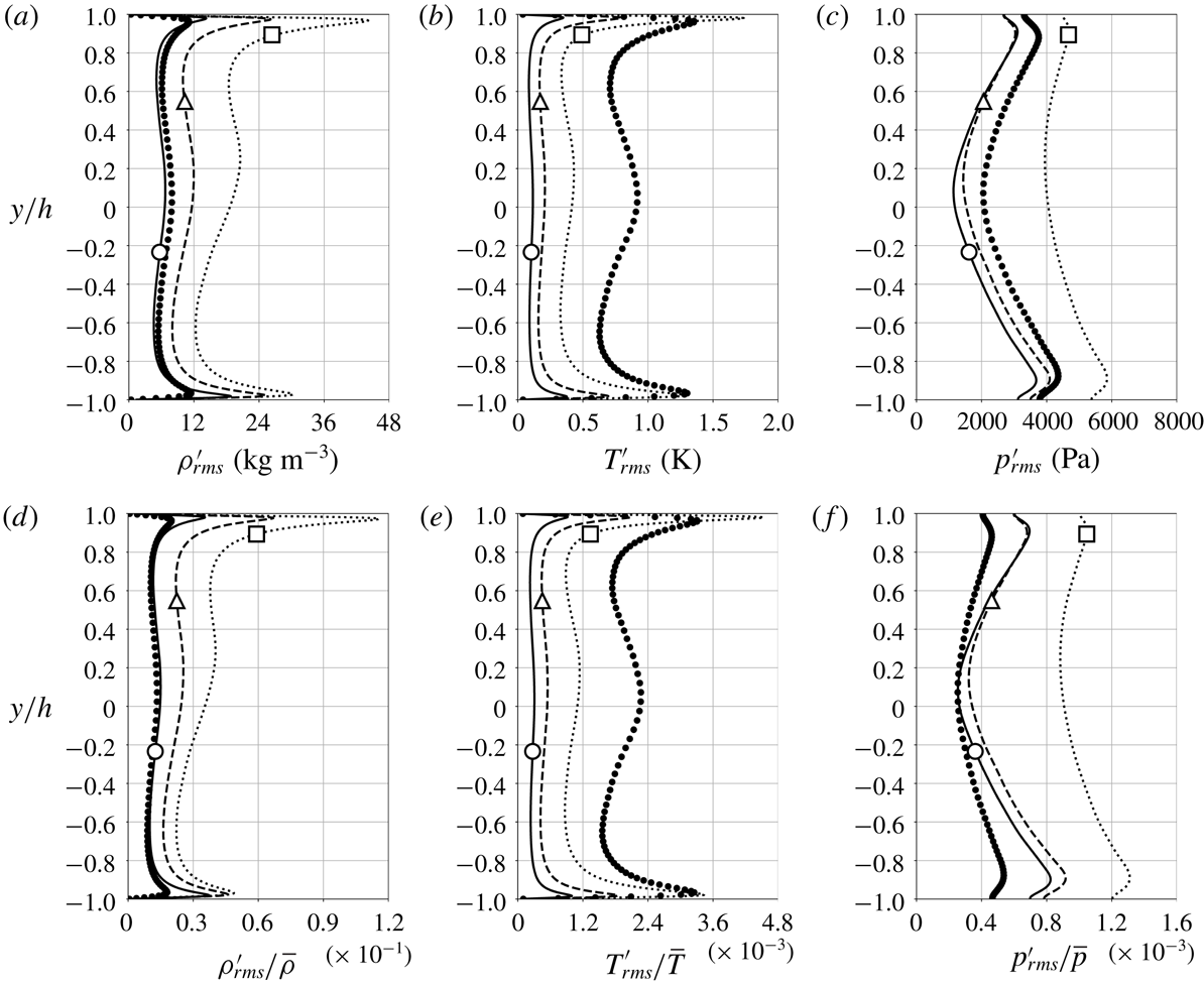
In all cases, the transition from a seemingly fully thermally mixed region in channel core (i.e.
 $\overline{T}(y)$
is relatively uniform and close to the pseudoboiling value) is more defined than in the reference simulation. Such steep mean flow gradients near the walls sustain significant density and enthalpy fluctuations, up to
$\overline{T}(y)$
is relatively uniform and close to the pseudoboiling value) is more defined than in the reference simulation. Such steep mean flow gradients near the walls sustain significant density and enthalpy fluctuations, up to
 $\unicode[STIX]{x1D70C}_{rms,max}=44.1~\text{kg}~\text{m}^{-3}$
and
$\unicode[STIX]{x1D70C}_{rms,max}=44.1~\text{kg}~\text{m}^{-3}$
and
 $h_{rms,max}=8.9~\text{kJ}~\text{kg}^{-1}$
, respectively (as discussed later in figures 11 and 12) for the
$h_{rms,max}=8.9~\text{kJ}~\text{kg}^{-1}$
, respectively (as discussed later in figures 11 and 12) for the
 $\unicode[STIX]{x0394}T=20$
K case. The very high heat capacity of the fluid undergoing pseudophase transition, on the other hand, limits the temperature fluctuations to
$\unicode[STIX]{x0394}T=20$
K case. The very high heat capacity of the fluid undergoing pseudophase transition, on the other hand, limits the temperature fluctuations to
 $T_{rms,max}<2~\text{K}$
.
$T_{rms,max}<2~\text{K}$
.

Figure 5. Reynolds-averaged streamwise velocity component (a) and its wall-normal gradient (b) for
 $p_{b}=1.1p_{cr}$
and
$p_{b}=1.1p_{cr}$
and
 $\unicode[STIX]{x0394}T=5$
K (——), 10 K (- - -) and 20 K (
$\unicode[STIX]{x0394}T=5$
K (——), 10 K (- - -) and 20 K (
 $\cdots \cdots$
) and reference data for
$\cdots \cdots$
) and reference data for
 $p_{b}=2p_{cr}$
and
$p_{b}=2p_{cr}$
and
 $\unicode[STIX]{x0394}T=20$
K (●) (see § 2.3). Average location of pseudotransition for
$\unicode[STIX]{x0394}T=20$
K (●) (see § 2.3). Average location of pseudotransition for
 $\unicode[STIX]{x0394}T=5~\text{K}$
(○), 10 K (▵) and 20 K (▫).
$\unicode[STIX]{x0394}T=5~\text{K}$
(○), 10 K (▵) and 20 K (▫).

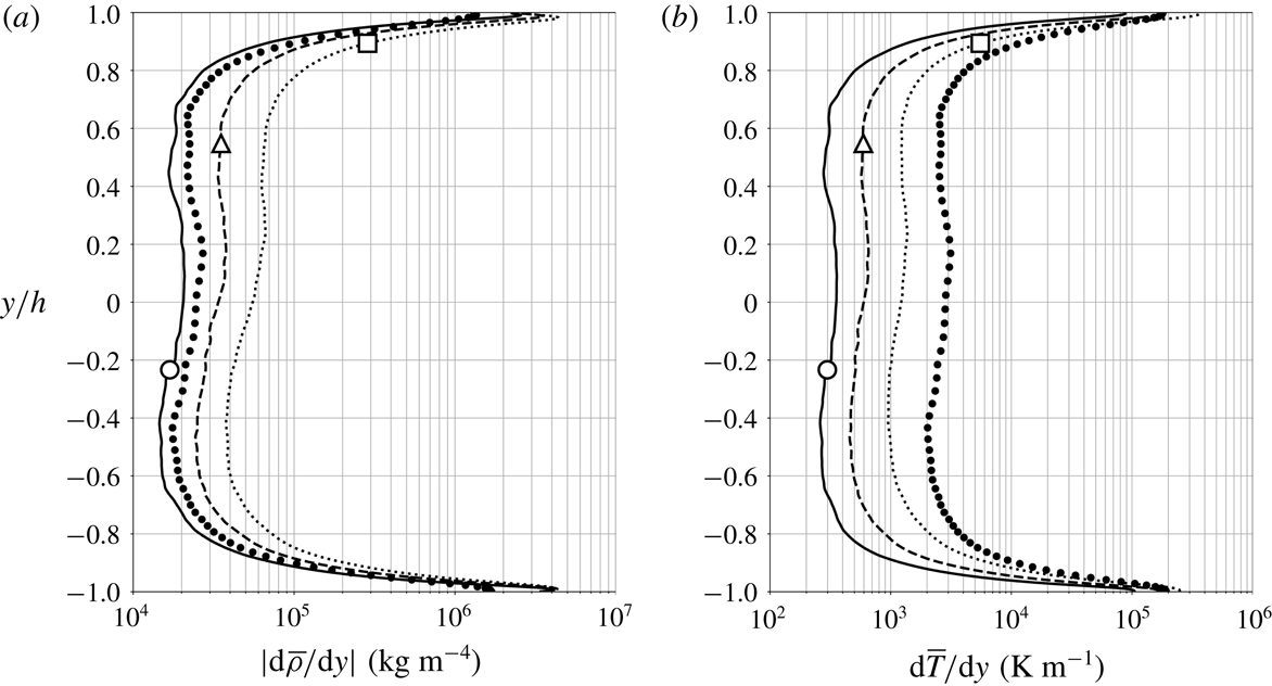
Figure 6. Wall-normal gradient of Reynolds-averaged mean density (a) and temperature (b) for
 $p_{b}=1.1p_{cr}$
and
$p_{b}=1.1p_{cr}$
and
 $\unicode[STIX]{x0394}T=5$
K (——), 10 K (- - -) and 20 K (
$\unicode[STIX]{x0394}T=5$
K (——), 10 K (- - -) and 20 K (
 $\cdots \cdots$
) and reference data for
$\cdots \cdots$
) and reference data for
 $p_{b}=2p_{cr}$
and
$p_{b}=2p_{cr}$
and
 $\unicode[STIX]{x0394}T=20$
K (●) (see § 2.3). Average location of pseudotransition for
$\unicode[STIX]{x0394}T=20$
K (●) (see § 2.3). Average location of pseudotransition for
 $\unicode[STIX]{x0394}T=5~\text{K}$
(○), 10 K (▵) and 20 K (▫).
$\unicode[STIX]{x0394}T=5~\text{K}$
(○), 10 K (▵) and 20 K (▫).
The mean turbulent streamwise velocity profile (figure 5
a) becomes more asymmetric (with a slight acceleration of the pseudogaseous layer) with increasing
 $\unicode[STIX]{x0394}T$
, with an upwards shift in the maximum velocity location,
$\unicode[STIX]{x0394}T$
, with an upwards shift in the maximum velocity location,
 $y/h=0.06$
for
$y/h=0.06$
for
 $\unicode[STIX]{x0394}T=5$
K, 0.11 for
$\unicode[STIX]{x0394}T=5$
K, 0.11 for
 $\unicode[STIX]{x0394}T=10$
K and 0.17 for
$\unicode[STIX]{x0394}T=10$
K and 0.17 for
 $\unicode[STIX]{x0394}T=20$
K (see inset in figure 5
b), following the same trend of the pseudotransition location,
$\unicode[STIX]{x0394}T=20$
K (see inset in figure 5
b), following the same trend of the pseudotransition location,
 $y_{pb}$
. As a result, a larger velocity gradient magnitude is found near the top wall (the magnitude ratio of top-to-bottom velocity gradient is 1.24 for
$y_{pb}$
. As a result, a larger velocity gradient magnitude is found near the top wall (the magnitude ratio of top-to-bottom velocity gradient is 1.24 for
 $\unicode[STIX]{x0394}T=5$
K, 1.32 for
$\unicode[STIX]{x0394}T=5$
K, 1.32 for
 $\unicode[STIX]{x0394}T=10$
K, 1.44 for
$\unicode[STIX]{x0394}T=10$
K, 1.44 for
 $\unicode[STIX]{x0394}T=20$
K in figure 5
b). In figure 6, while top-down asymmetries in the temperature gradient are confined to the sublayer regions, the mean density gradient profile is more visibly affected by the location of pseudotransition. A logarithmic increment of the centreplane of the temperature gradient is observed as
$\unicode[STIX]{x0394}T=20$
K in figure 5
b). In figure 6, while top-down asymmetries in the temperature gradient are confined to the sublayer regions, the mean density gradient profile is more visibly affected by the location of pseudotransition. A logarithmic increment of the centreplane of the temperature gradient is observed as
 $\unicode[STIX]{x0394}T$
is also increased logarithmically (i.e.
$\unicode[STIX]{x0394}T$
is also increased logarithmically (i.e.
 $\text{d}(\unicode[STIX]{x0394}T)/\unicode[STIX]{x0394}T=\text{const.}$
), suggesting a linear relation between the overall top-to-bottom equilibrium heat flux and
$\text{d}(\unicode[STIX]{x0394}T)/\unicode[STIX]{x0394}T=\text{const.}$
), suggesting a linear relation between the overall top-to-bottom equilibrium heat flux and
 $\unicode[STIX]{x0394}T$
. The latter is a surprising result given that the level of hydrodynamic and thermodynamic nonlinearity of the problem. These results also suggest that transcritical heat flux rates are amenable to straightforward dimensionless scaling in similar canonical set-ups. While the velocity gradient increase (decrease) in the pseudogaseous (pseudoliquid) region as
$\unicode[STIX]{x0394}T$
. The latter is a surprising result given that the level of hydrodynamic and thermodynamic nonlinearity of the problem. These results also suggest that transcritical heat flux rates are amenable to straightforward dimensionless scaling in similar canonical set-ups. While the velocity gradient increase (decrease) in the pseudogaseous (pseudoliquid) region as
 $\unicode[STIX]{x0394}T$
is increased is not as significant as the corresponding variations in density and temperature gradients, the real fluid effects are very apparent when attempting to scale the mean velocity profiles with commonly used scaling laws.
$\unicode[STIX]{x0394}T$
is increased is not as significant as the corresponding variations in density and temperature gradients, the real fluid effects are very apparent when attempting to scale the mean velocity profiles with commonly used scaling laws.
Table 4. Semi-local scaling factors where
 $\overline{u}_{\unicode[STIX]{x1D70F}}^{\ast }(y)=\sqrt{\overline{\unicode[STIX]{x1D70F}}_{w}/\overline{\unicode[STIX]{x1D70C}}(y)}$
.
$\overline{u}_{\unicode[STIX]{x1D70F}}^{\ast }(y)=\sqrt{\overline{\unicode[STIX]{x1D70F}}_{w}/\overline{\unicode[STIX]{x1D70C}}(y)}$
.

For all
 $\unicode[STIX]{x0394}T$
values, the mean streamwise velocity profiles are scaled following the recently proposed approach by Trettel & Larsson (Reference Trettel and Larsson2016) which accounts for the wall heat transfer effects, the van Driest transformation (van Driest Reference van Driest1951) and the semi-local scaling (Huang et al.
Reference Huang, Coleman and Bradshaw1995) (figure 7). The expressions of the three transformations considered are reported here for convenience and completeness.
$\unicode[STIX]{x0394}T$
values, the mean streamwise velocity profiles are scaled following the recently proposed approach by Trettel & Larsson (Reference Trettel and Larsson2016) which accounts for the wall heat transfer effects, the van Driest transformation (van Driest Reference van Driest1951) and the semi-local scaling (Huang et al.
Reference Huang, Coleman and Bradshaw1995) (figure 7). The expressions of the three transformations considered are reported here for convenience and completeness.

Figure 7. Mean streamwise velocity versus wall-normal coordinate in wall units scaled based on the conventional van Driest transformation plotted against wall-normal distance in classic wall units (a) and semi-locally scaled (Huang et al.
Reference Huang, Coleman and Bradshaw1995) (b), transformed following Trettel & Larsson (Reference Trettel and Larsson2016) (c) for
 $p_{b}=1.1p_{cr}$
and
$p_{b}=1.1p_{cr}$
and
 $\unicode[STIX]{x0394}T=5$
K (——, thickened), 10 K (- - -) and 20 K (
$\unicode[STIX]{x0394}T=5$
K (——, thickened), 10 K (- - -) and 20 K (
 $\cdots \cdots$
); reference data for
$\cdots \cdots$
); reference data for
 $p_{b}=2p_{cr}$
and
$p_{b}=2p_{cr}$
and
 $\unicode[STIX]{x0394}T=20$
K (circles); bottom wall (blue, ●) and top wall (red, ○). Profiles of the law of the wall (
$\unicode[STIX]{x0394}T=20$
K (circles); bottom wall (blue, ●) and top wall (red, ○). Profiles of the law of the wall (
 $\overline{u}^{+}=y^{+}$
for the viscous sublayer;
$\overline{u}^{+}=y^{+}$
for the viscous sublayer;
 $\overline{u}^{+}=1/\unicode[STIX]{x1D705}\ln y^{+}+C$
, where
$\overline{u}^{+}=1/\unicode[STIX]{x1D705}\ln y^{+}+C$
, where
 $\unicode[STIX]{x1D705}=0.41$
and
$\unicode[STIX]{x1D705}=0.41$
and
 $C=5.2$
for the log-law region) are shown with a thin solid black line for reference.
$C=5.2$
for the log-law region) are shown with a thin solid black line for reference.
The van Driest transformation (van Driest Reference van Driest1951) is given by
 $$\begin{eqnarray}\displaystyle \overline{u}_{VD}^{+}=\int _{0}^{\overline{u}^{+}}\left(\frac{\overline{\unicode[STIX]{x1D70C}}(y)}{\overline{\unicode[STIX]{x1D70C}}_{w}}\right)^{1/2}\,\text{d}\overline{u}^{+}, & & \displaystyle\end{eqnarray}$$
where
 $\overline{u}^{+}=\overline{u}(y)/\overline{u}_{\unicode[STIX]{x1D70F}}$
and the conventional set of scaling parameters reads
$\overline{u}^{+}=\overline{u}(y)/\overline{u}_{\unicode[STIX]{x1D70F}}$
and the conventional set of scaling parameters reads
 $$\begin{eqnarray}\displaystyle y^{+}=\frac{y}{\unicode[STIX]{x1D6FF}_{v}}=\frac{y}{\overline{\unicode[STIX]{x1D707}}_{w}/(\overline{\unicode[STIX]{x1D70C}}_{w}\overline{u}_{\unicode[STIX]{x1D70F}})},\quad \overline{u}_{\unicode[STIX]{x1D70F}}=\sqrt{\overline{\unicode[STIX]{x1D70F}}_{w}/\overline{\unicode[STIX]{x1D70C}}_{w}}, & & \displaystyle\end{eqnarray}$$
whereas, for the semi-local scaling (Huang et al. Reference Huang, Coleman and Bradshaw1995), it reads
 $$\begin{eqnarray}\displaystyle y^{\ast }=\frac{y}{\unicode[STIX]{x1D6FF}_{v}^{\ast }}=\frac{y}{\overline{\unicode[STIX]{x1D707}}(y)/(\overline{\unicode[STIX]{x1D70C}}(y)\overline{u}_{\unicode[STIX]{x1D70F}}^{\ast }(y))},\quad \overline{u}_{\unicode[STIX]{x1D70F}}^{\ast }(y)=\sqrt{\overline{\unicode[STIX]{x1D70F}}_{w}/\overline{\unicode[STIX]{x1D70C}}(y)}, & & \displaystyle\end{eqnarray}$$
and its factors for various quantities are shown in table 4.

Figure 8. Semi-local friction Reynolds number at the bottom (a) and top (b) wall for
 $p_{b}=1.1p_{cr}$
and
$p_{b}=1.1p_{cr}$
and
 $\unicode[STIX]{x0394}T=5$
K (——), 10 K (- - -) and 20 K (
$\unicode[STIX]{x0394}T=5$
K (——), 10 K (- - -) and 20 K (
 $\cdots \cdots$
).
$\cdots \cdots$
).
Finally, the transformation by Trettel & Larsson (Reference Trettel and Larsson2016) reads
 $$\begin{eqnarray}\displaystyle \overline{u}_{TL}^{+}=\int _{0}^{\overline{u}^{+}}\left(\frac{\overline{\unicode[STIX]{x1D70C}}(y)}{\overline{\unicode[STIX]{x1D70C}}_{w}}\right)^{1/2}\left[1+\frac{1}{2}\frac{1}{\overline{\unicode[STIX]{x1D70C}}(y)}\frac{\text{d}\overline{\unicode[STIX]{x1D70C}}(y)}{\text{d}y}y-\frac{1}{\overline{\unicode[STIX]{x1D707}}(y)}\frac{\text{d}\overline{\unicode[STIX]{x1D707}}(y)}{\text{d}y}y\right]\text{d}\overline{u}^{+}. & & \displaystyle\end{eqnarray}$$
While the reference results at
 $p_{b}=2p_{cr}$
collapse profiles from both walls in the log-law region with the Trettel & Larsson (Reference Trettel and Larsson2016) transformation, the widest spread is observed with the semi-local scaling. The transformed top- and bottom-wall streamwise velocity profiles at transcritical temperature conditions result in higher intercepts than the classic incompressible log-law as the pressure increases. In the recent publication by Ma et al. (Reference Ma, Yang and Ihme2018) replicating our same set-up, very large values of the transformed velocity
$p_{b}=2p_{cr}$
collapse profiles from both walls in the log-law region with the Trettel & Larsson (Reference Trettel and Larsson2016) transformation, the widest spread is observed with the semi-local scaling. The transformed top- and bottom-wall streamwise velocity profiles at transcritical temperature conditions result in higher intercepts than the classic incompressible log-law as the pressure increases. In the recent publication by Ma et al. (Reference Ma, Yang and Ihme2018) replicating our same set-up, very large values of the transformed velocity
 $\overline{u}_{TL}^{+}$
in the log region were obtained by erroneously adopting a semi-locally scaled velocity differential in (3.5), suggesting inadequacy of this transformation for this flow. The present results show, instead, an acceptable collapse using the Trettel & Larsson (Reference Trettel and Larsson2016) transformation.
$\overline{u}_{TL}^{+}$
in the log region were obtained by erroneously adopting a semi-locally scaled velocity differential in (3.5), suggesting inadequacy of this transformation for this flow. The present results show, instead, an acceptable collapse using the Trettel & Larsson (Reference Trettel and Larsson2016) transformation.
Effects of varying
 $\unicode[STIX]{x0394}T$
are visible (hence not collapsed perfectly) in all adopted transformations. Increasing
$\unicode[STIX]{x0394}T$
are visible (hence not collapsed perfectly) in all adopted transformations. Increasing
 $\unicode[STIX]{x0394}T$
results in an enhancement of real fluid effects (at the present conditions) yielding variations of the state of turbulence in the wall-normal direction, analysed below via extraction of the semi-local friction Reynolds number and density fluctuation intensity profiles.
$\unicode[STIX]{x0394}T$
results in an enhancement of real fluid effects (at the present conditions) yielding variations of the state of turbulence in the wall-normal direction, analysed below via extraction of the semi-local friction Reynolds number and density fluctuation intensity profiles.
Figure 8 shows the semi-local friction Reynolds number
 $$\begin{eqnarray}\displaystyle \overline{Re}_{\unicode[STIX]{x1D70F}}^{\ast }=\overline{Re}_{\unicode[STIX]{x1D70F}}\sqrt{\overline{\unicode[STIX]{x1D70C}}(y)/\overline{\unicode[STIX]{x1D70C}}_{w}}/(\overline{\unicode[STIX]{x1D707}}(y)/\overline{\unicode[STIX]{x1D707}}_{w}), & & \displaystyle\end{eqnarray}$$
where
 $\overline{Re}_{\unicode[STIX]{x1D70F}}=\overline{\unicode[STIX]{x1D70C}}_{w}\overline{u}_{\unicode[STIX]{x1D70F}}h/\overline{\unicode[STIX]{x1D707}}_{w}$
and the semi-locally scaled wall-normal coordinate,
$\overline{Re}_{\unicode[STIX]{x1D70F}}=\overline{\unicode[STIX]{x1D70C}}_{w}\overline{u}_{\unicode[STIX]{x1D70F}}h/\overline{\unicode[STIX]{x1D707}}_{w}$
and the semi-locally scaled wall-normal coordinate,
 $y^{\ast }$
, is here intended as the relative distance from either the top or the bottom wall. The values of
$y^{\ast }$
, is here intended as the relative distance from either the top or the bottom wall. The values of
 $\overline{Re}_{\unicode[STIX]{x1D70F}}^{\ast }$
in the bottom-wall viscous sublayer are lower than those near the top wall; the opposite occurs in the respective log-law regions. However, values of
$\overline{Re}_{\unicode[STIX]{x1D70F}}^{\ast }$
in the bottom-wall viscous sublayer are lower than those near the top wall; the opposite occurs in the respective log-law regions. However, values of
 $\overline{Re}_{\unicode[STIX]{x1D70F},bot}^{\ast }$
in the log-law region are comparable across the different
$\overline{Re}_{\unicode[STIX]{x1D70F},bot}^{\ast }$
in the log-law region are comparable across the different
 $\unicode[STIX]{x0394}T$
considered, while
$\unicode[STIX]{x0394}T$
considered, while
 $\overline{Re}_{\unicode[STIX]{x1D70F},top}^{\ast }$
systematically decreases in the respective log-law region as
$\overline{Re}_{\unicode[STIX]{x1D70F},top}^{\ast }$
systematically decreases in the respective log-law region as
 $\unicode[STIX]{x0394}T$
increases (and as the pseudophase transitioning region of the flow approaches the top-wall buffer layer). The overall higher sensitivity of
$\unicode[STIX]{x0394}T$
increases (and as the pseudophase transitioning region of the flow approaches the top-wall buffer layer). The overall higher sensitivity of
 $\overline{Re}_{\unicode[STIX]{x1D70F}}^{\ast }$
to
$\overline{Re}_{\unicode[STIX]{x1D70F}}^{\ast }$
to
 $\unicode[STIX]{x0394}T$
on the heated top wall is manifest in the van Driest transformed velocity (figure 7
a,b) showing the systematic increase in value with
$\unicode[STIX]{x0394}T$
on the heated top wall is manifest in the van Driest transformed velocity (figure 7
a,b) showing the systematic increase in value with
 $\unicode[STIX]{x0394}T$
for the top wall more than the bottom wall. Also, as noted by Patel, Boersma & Pecnik (Reference Patel, Boersma and Pecnik2016), the van Driest transformed velocity profiles plotted as a function of
$\unicode[STIX]{x0394}T$
for the top wall more than the bottom wall. Also, as noted by Patel, Boersma & Pecnik (Reference Patel, Boersma and Pecnik2016), the van Driest transformed velocity profiles plotted as a function of
 $y^{\ast }$
in figure 7(b) for the bottom-wall region resemble the profiles of
$y^{\ast }$
in figure 7(b) for the bottom-wall region resemble the profiles of
 $\overline{Re}_{\unicode[STIX]{x1D70F},bot}^{\ast }$
and the inverse of
$\overline{Re}_{\unicode[STIX]{x1D70F},bot}^{\ast }$
and the inverse of
 $\overline{Re}_{\unicode[STIX]{x1D70F},top}^{\ast }$
(vice versa for the top wall). Changes in mean velocity profiles, as well as in the turbulence, are related to wall-normal variations of
$\overline{Re}_{\unicode[STIX]{x1D70F},top}^{\ast }$
(vice versa for the top wall). Changes in mean velocity profiles, as well as in the turbulence, are related to wall-normal variations of
 $\overline{Re}_{\unicode[STIX]{x1D70F}}^{\ast }$
. On the other hand, the Trettel & Larsson transformed profiles collapse the data across the various
$\overline{Re}_{\unicode[STIX]{x1D70F}}^{\ast }$
. On the other hand, the Trettel & Larsson transformed profiles collapse the data across the various
 $\unicode[STIX]{x0394}T$
cases considered, in equal manners on both walls, despite the real fluid effects being more pronounced at the top wall (as also discussed later and illustrated in figures 12 and 13).
$\unicode[STIX]{x0394}T$
cases considered, in equal manners on both walls, despite the real fluid effects being more pronounced at the top wall (as also discussed later and illustrated in figures 12 and 13).
Although the Trettel & Larsson transform results in a collapse between the top and bottom walls for a given simulation (or given
 $\unicode[STIX]{x0394}T$
), we do note a non-negligible spread among the simulations. More specifically, the same slope in the log law is obtained, but the intercept value increases with the wall-to-wall temperature difference. Such spread in the intercept values (compared to a universal profile) can arise either due to the error in the derivation of the stress balance condition or due the log-law assumptions; both are investigated here.
$\unicode[STIX]{x0394}T$
), we do note a non-negligible spread among the simulations. More specifically, the same slope in the log law is obtained, but the intercept value increases with the wall-to-wall temperature difference. Such spread in the intercept values (compared to a universal profile) can arise either due to the error in the derivation of the stress balance condition or due the log-law assumptions; both are investigated here.
In regard to the closure of the stress balance, all the above wall scaling models rely on Morkovin’s hypothesis, which assumes that the compressibility effects on turbulence are only related to the mean density variations, not the density fluctuations. Further, all the scalings neglect the correlation between the viscosity and fluctuating velocity derivative as a component of the total shear. These hypotheses are evoked to simplify the near-wall stress balance, yielding
 $$\begin{eqnarray}\displaystyle \overline{\unicode[STIX]{x1D707}\frac{\unicode[STIX]{x2202}u}{\unicode[STIX]{x2202}y}}-\overline{\unicode[STIX]{x1D70C}u^{\prime }v^{\prime }}\approx \overline{\unicode[STIX]{x1D707}}\frac{\unicode[STIX]{x2202}\overline{u}}{\unicode[STIX]{x2202}y}-\overline{\unicode[STIX]{x1D70C}}\overline{u^{\prime }v^{\prime }}+\underbrace{\overline{\unicode[STIX]{x1D707}^{\prime }\frac{\unicode[STIX]{x2202}u^{\prime }}{\unicode[STIX]{x2202}y}}-\overline{\unicode[STIX]{x1D70C}^{\prime }u^{\prime }v^{\prime }}}_{}=\unicode[STIX]{x1D70F}_{w}. & & \displaystyle\end{eqnarray}$$
For ideal-gas flows in the subsonic and low-supersonic regime, the terms highlighted by the underbrace are negligible. In the transcritical regime, where the fluctuations of viscosity and density are significant, the error due to neglecting
 $\overline{\unicode[STIX]{x1D707}^{\prime }(\unicode[STIX]{x2202}u^{\prime }/\unicode[STIX]{x2202}y)}$
and
$\overline{\unicode[STIX]{x1D707}^{\prime }(\unicode[STIX]{x2202}u^{\prime }/\unicode[STIX]{x2202}y)}$
and
 $\overline{\unicode[STIX]{x1D70C}^{\prime }u^{\prime }v^{\prime }}$
may be significant. In the simulations presented herein, they are, respectively, up to 2 % and 5 % of the total shear (for
$\overline{\unicode[STIX]{x1D70C}^{\prime }u^{\prime }v^{\prime }}$
may be significant. In the simulations presented herein, they are, respectively, up to 2 % and 5 % of the total shear (for
 $\unicode[STIX]{x0394}T=20$
K). This makes Morkovin’s hypothesis and the assumption of negligible viscosity fluctuation correlations questionable for the low-speed transcritical flows analysed herein.
$\unicode[STIX]{x0394}T=20$
K). This makes Morkovin’s hypothesis and the assumption of negligible viscosity fluctuation correlations questionable for the low-speed transcritical flows analysed herein.
We now move on to considering the assumptions underlying the log law. Its intercept value corresponds to the integration constant in the scaled velocity profile (Marusic et al. Reference Marusic, Monty, Hultmark and Smits2013), and is known to vary for wall roughness (Bradshaw Reference Bradshaw1994), heated (Lee et al. Reference Lee, Jung, Sung and Zaki2013) or superhydrophobic (Min & Kim Reference Min and Kim2004) boundary-layer flows. Therefore, the intercept value is highly dependent on the near-wall conditions. Using dimensional scaling arguments, Bradshaw (Reference Bradshaw1994) argues that the velocity derivative in the log layer is proportional to a velocity scale (friction velocity) and inversely to the wall distance:
 $$\begin{eqnarray}\displaystyle \frac{\text{d}u}{\text{d}y}=\frac{1}{\unicode[STIX]{x1D705}}\frac{1}{y}u_{\unicode[STIX]{x1D70F}}. & & \displaystyle\end{eqnarray}$$
In the compressible regime, a heuristic argument (Bradshaw Reference Bradshaw1994) is evoked in which the friction factor is replaced by a locally varying velocity scale (Trettel & Larsson Reference Trettel and Larsson2016):
 $$\begin{eqnarray}\displaystyle \frac{\text{d}u}{\text{d}y}=\frac{1}{\unicode[STIX]{x1D705}}\frac{1}{y}\left(\frac{\unicode[STIX]{x1D70F}_{w}}{\overline{\unicode[STIX]{x1D70C}}}\right)^{1/2}. & & \displaystyle\end{eqnarray}$$
The above equation, along with the stress-balance condition, is central to the Trettel & Larsson transform. When assessing the validity of (3.9) in the transcritical flows analysed herein, we note a significant relative error in the log region when applying the above relation. The error is above 20 % in the log layer in the bottom portion of the channel for
 $\unicode[STIX]{x0394}T=20$
K; the error on the top half of the channel is even more significant. In other words, this observation informs us that the selection of the characteristic velocity scales within the van Driest and Trettel & Larsson derivation of the log-law conditions is not straightforwardly extendable to transcritical flows.
$\unicode[STIX]{x0394}T=20$
K; the error on the top half of the channel is even more significant. In other words, this observation informs us that the selection of the characteristic velocity scales within the van Driest and Trettel & Larsson derivation of the log-law conditions is not straightforwardly extendable to transcritical flows.
3.2 Turbulent fluctuation intensities

Figure 9. Root-mean-square of streamwise (a), wall-normal (b) and spanwise (c) Favre fluctuating velocity component and Reynolds shear stress (d) for
 $p_{b}=1.1p_{cr}$
and
$p_{b}=1.1p_{cr}$
and
 $\unicode[STIX]{x0394}T=5$
K (——), 10 K (- - -) and 20 K (
$\unicode[STIX]{x0394}T=5$
K (——), 10 K (- - -) and 20 K (
 $\cdots \cdots$
) and reference data for
$\cdots \cdots$
) and reference data for
 $p_{b}=2p_{cr}$
and
$p_{b}=2p_{cr}$
and
 $\unicode[STIX]{x0394}T=20$
K (●) (see § 2.3). Average location of pseudotransition for
$\unicode[STIX]{x0394}T=20$
K (●) (see § 2.3). Average location of pseudotransition for
 $\unicode[STIX]{x0394}T=5~\text{K}$
(○), 10 K (▵) and 20 K (▫).
$\unicode[STIX]{x0394}T=5~\text{K}$
(○), 10 K (▵) and 20 K (▫).
Table 5. Top-to-bottom difference in root-mean-square peak values of streamwise, wall-normal and spanwise velocity components, density, temperature and pressure as percentage of the bottom peak root-mean-square value.


Figure 10. Semi-local scaled root-mean-square of streamwise, wall-normal and spanwise Favre fluctuating velocity component (a,c) and Reynolds shear stress (b,d) at the bottom (a,b) and top (c,d) wall for
 $p_{b}=1.1p_{cr}$
and
$p_{b}=1.1p_{cr}$
and
 $\unicode[STIX]{x0394}T=5$
K (——), 10 K (- - -) and 20 K (
$\unicode[STIX]{x0394}T=5$
K (——), 10 K (- - -) and 20 K (
 $\cdots \cdots$
) and reference data for
$\cdots \cdots$
) and reference data for
 $p_{b}=2p_{cr}$
and
$p_{b}=2p_{cr}$
and
 $\unicode[STIX]{x0394}T=20$
K (●) (see § 2.3). Semi-local scaling factors are given in table 4.
$\unicode[STIX]{x0394}T=20$
K (●) (see § 2.3). Semi-local scaling factors are given in table 4.
Other real fluid effects associated with transcritical thermal conditions are observable in the variance of the hydrodynamic turbulent fluctuations as shown in figure 9. As
 $\unicode[STIX]{x0394}T$
increases, the asymmetries with respect to the channel centreplane grow and the peak fluctuation intensity values at the top wall (pseudogaseous region towards which the pseudotransition location migrates) are attenuated corresponding to the values in the pseudoliquid flow as shown in table 5. This suggests the occurrence of damping of hydrodynamic turbulence due to the proximity to the region of pseudophase change. Such attenuation is noted in all Reynolds stress terms, but is strongest in the wall-normal velocity component, directly involved in the turbulent heat and mass transport working against the steep mean temperature and density gradient. Following Morinishi, Tamano & Nakabayashi (Reference Morinishi, Tamano and Nakabayashi2004), in figure 10 we show the semi-local scaled profiles of turbulent velocity fluctuations (see table 4 for the semi-local scaling factors). The semi-local scaling collapses well the high-pressure data
$\unicode[STIX]{x0394}T$
increases, the asymmetries with respect to the channel centreplane grow and the peak fluctuation intensity values at the top wall (pseudogaseous region towards which the pseudotransition location migrates) are attenuated corresponding to the values in the pseudoliquid flow as shown in table 5. This suggests the occurrence of damping of hydrodynamic turbulence due to the proximity to the region of pseudophase change. Such attenuation is noted in all Reynolds stress terms, but is strongest in the wall-normal velocity component, directly involved in the turbulent heat and mass transport working against the steep mean temperature and density gradient. Following Morinishi, Tamano & Nakabayashi (Reference Morinishi, Tamano and Nakabayashi2004), in figure 10 we show the semi-local scaled profiles of turbulent velocity fluctuations (see table 4 for the semi-local scaling factors). The semi-local scaling collapses well the high-pressure data
 $2p_{cr}$
onto the near-critical
$2p_{cr}$
onto the near-critical
 $1.1p_{cr}$
cases, with the exception of the streamwise velocity fluctuations; a much better collapse is observed across the various
$1.1p_{cr}$
cases, with the exception of the streamwise velocity fluctuations; a much better collapse is observed across the various
 $\unicode[STIX]{x0394}T$
conditions for the same near-critical case in terms of the peak value level and its location in the semi-local wall unit,
$\unicode[STIX]{x0394}T$
conditions for the same near-critical case in terms of the peak value level and its location in the semi-local wall unit,
 $y^{\ast }$
(see table 6).
$y^{\ast }$
(see table 6).
Table 6. Peak ranges of the root-mean-square of streamwise, wall-normal and spanwise Favre fluctuating velocity component and Reynolds shear stress at the bottom and top wall and their wall-normal location using the semi-local scaling.

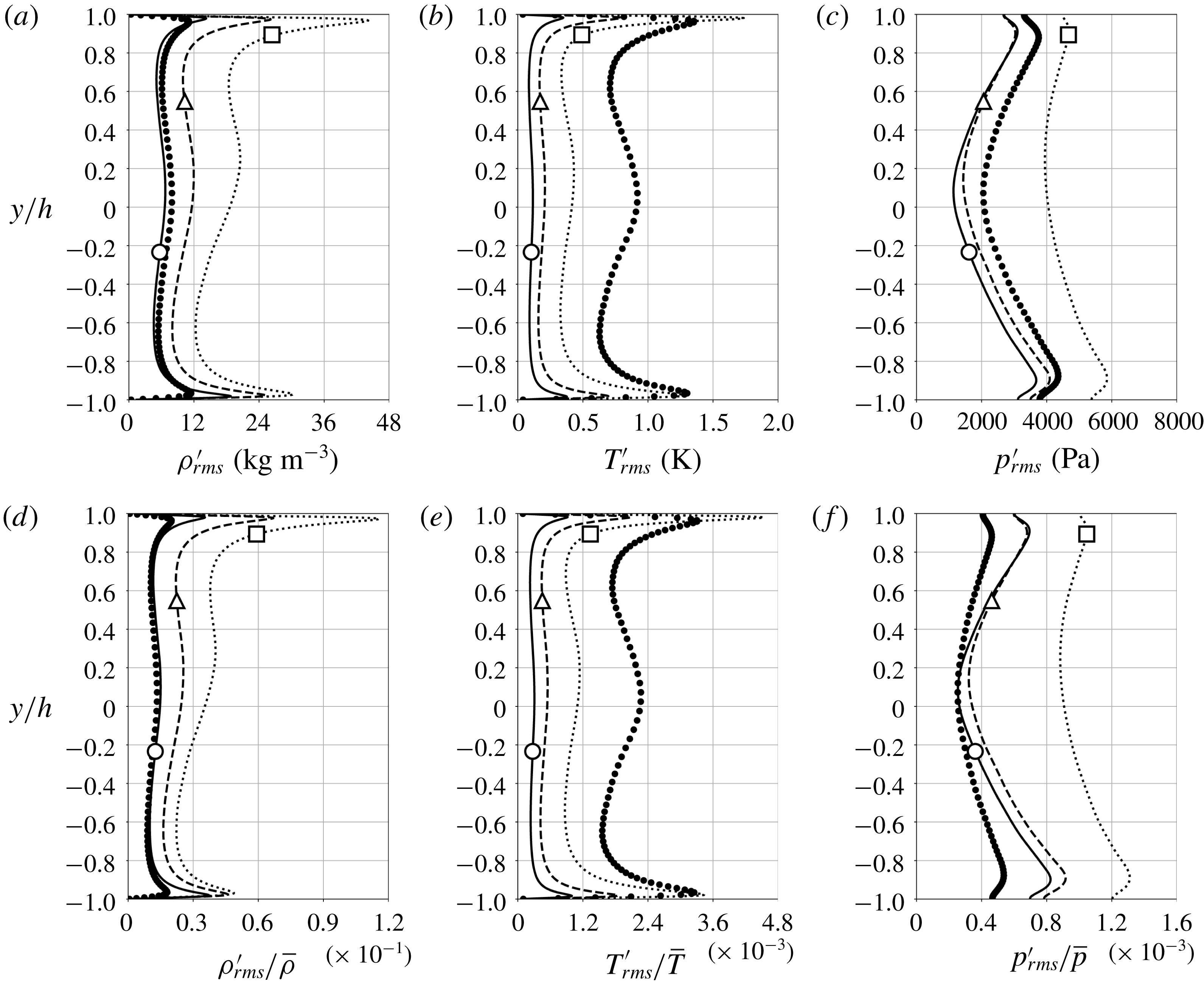
Figure 11. Root-mean-square of Reynolds fluctuations (a–c) and their normalized quantities (d–f) with respect to the local mean values for density (a,d), temperature (b,e) and pressure (c,f) for
 $p_{b}=1.1p_{cr}$
and
$p_{b}=1.1p_{cr}$
and
 $\unicode[STIX]{x0394}T=5$
K (——), 10 K (- - -) and 20 K (
$\unicode[STIX]{x0394}T=5$
K (——), 10 K (- - -) and 20 K (
 $\cdots \cdots$
) and reference data for
$\cdots \cdots$
) and reference data for
 $p_{b}=2p_{cr}$
and
$p_{b}=2p_{cr}$
and
 $\unicode[STIX]{x0394}T=20$
K (●) (see § 2.3). Average location of pseudotransition for
$\unicode[STIX]{x0394}T=20$
K (●) (see § 2.3). Average location of pseudotransition for
 $\unicode[STIX]{x0394}T=5~\text{K}$
(○), 10 K (▵) and 20 K (▫).
$\unicode[STIX]{x0394}T=5~\text{K}$
(○), 10 K (▵) and 20 K (▫).

Figure 12. Root-mean-square of Favre fluctuations for enthalpy (a) and wall-normal turbulent enthalpy flux (b) for
 $p_{b}=1.1p_{cr}$
and
$p_{b}=1.1p_{cr}$
and
 $\unicode[STIX]{x0394}T=5$
K (——), 10 K (- - -) and 20 K (
$\unicode[STIX]{x0394}T=5$
K (——), 10 K (- - -) and 20 K (
 $\cdots \cdots$
). Average location of pseudotransition for
$\cdots \cdots$
). Average location of pseudotransition for
 $\unicode[STIX]{x0394}T=5~\text{K}$
(○), 10 K (▵) and 20 K (▫).
$\unicode[STIX]{x0394}T=5~\text{K}$
(○), 10 K (▵) and 20 K (▫).

Figure 13. Semi-local scaled root-mean-square of Reynolds fluctuating density at the bottom (a) and top (b) wall for
 $p_{b}=1.1p_{cr}$
and
$p_{b}=1.1p_{cr}$
and
 $\unicode[STIX]{x0394}T=5$
K (——), 10 K (- - -) and 20 K (
$\unicode[STIX]{x0394}T=5$
K (——), 10 K (- - -) and 20 K (
 $\cdots \cdots$
) and reference data for
$\cdots \cdots$
) and reference data for
 $p_{b}=2p_{cr}$
and
$p_{b}=2p_{cr}$
and
 $\unicode[STIX]{x0394}T=20$
K (●) (see § 2.3). Semi-local scaling factors are shown in table 4.
$\unicode[STIX]{x0394}T=20$
K (●) (see § 2.3). Semi-local scaling factors are shown in table 4.
On the contrary, the proximity to the pseudophase change location
 $y_{pb}$
(locally) and the increasing top-to-bottom temperature difference
$y_{pb}$
(locally) and the increasing top-to-bottom temperature difference
 $\unicode[STIX]{x0394}T$
(globally) enhance the intensity of all thermodynamic fluctuations (figures 11 and 12
a). In spite of damping in the wall-normal velocity fluctuations, the wall-normal turbulent enthalpy flux is enhanced (figure 12
b) by increasing
$\unicode[STIX]{x0394}T$
(globally) enhance the intensity of all thermodynamic fluctuations (figures 11 and 12
a). In spite of damping in the wall-normal velocity fluctuations, the wall-normal turbulent enthalpy flux is enhanced (figure 12
b) by increasing
 $\unicode[STIX]{x0394}T$
, as expected by the statistical steadiness of the flow, implying equilibrium conditions for the turbulent heat transfer.
$\unicode[STIX]{x0394}T$
, as expected by the statistical steadiness of the flow, implying equilibrium conditions for the turbulent heat transfer.
For any given
 $\unicode[STIX]{x0394}T$
, the root-mean-square peak of density, temperature and enthalpy closer to the location of pseudophase transition,
$\unicode[STIX]{x0394}T$
, the root-mean-square peak of density, temperature and enthalpy closer to the location of pseudophase transition,
 $y_{pb}$
, has a higher value than that farther away. This is not surprising as the thermophysical gradients are the largest at
$y_{pb}$
, has a higher value than that farther away. This is not surprising as the thermophysical gradients are the largest at
 $y\sim y_{pb}$
(see figure 1), and therefore pseudoboiling conditions are expected to enhance the local thermodynamic fluctuations, concomitantly enhancing the asymmetry in the fluctuating profiles; in fact, based on the transport equation for density variance (Chassaing et al.
Reference Chassaing, Antonia, Anselmet, Joly and Sarkar2013), the mean density gradient is responsible for production of density fluctuations, consistently with the data presented in this paper. Moreover, as
$y\sim y_{pb}$
(see figure 1), and therefore pseudoboiling conditions are expected to enhance the local thermodynamic fluctuations, concomitantly enhancing the asymmetry in the fluctuating profiles; in fact, based on the transport equation for density variance (Chassaing et al.
Reference Chassaing, Antonia, Anselmet, Joly and Sarkar2013), the mean density gradient is responsible for production of density fluctuations, consistently with the data presented in this paper. Moreover, as
 $y_{pb}$
moves upwards for increasing
$y_{pb}$
moves upwards for increasing
 $\unicode[STIX]{x0394}T$
, it approaches the peak of the shear Reynolds stress and enthalpy flux (figure 12
b), only significantly increasing the latter roughly proportionally to
$\unicode[STIX]{x0394}T$
, it approaches the peak of the shear Reynolds stress and enthalpy flux (figure 12
b), only significantly increasing the latter roughly proportionally to
 $\unicode[STIX]{x0394}T$
.
$\unicode[STIX]{x0394}T$
.
The density fluctuation intensity normalized by its mean local value shown in figure 11 is significantly higher than the temperature fluctuation (for
 $\unicode[STIX]{x0394}T=20$
K,
$\unicode[STIX]{x0394}T=20$
K,
 $(\unicode[STIX]{x1D70C}_{rms}^{\prime }/\overline{\unicode[STIX]{x1D70C}})_{max}\simeq 26\times (T_{rms}^{\prime }/\overline{T})_{max}$
). These real fluid effects have a direct impact on the structure of near-wall turbulence and are attenuated with increasing pressure.
$(\unicode[STIX]{x1D70C}_{rms}^{\prime }/\overline{\unicode[STIX]{x1D70C}})_{max}\simeq 26\times (T_{rms}^{\prime }/\overline{T})_{max}$
). These real fluid effects have a direct impact on the structure of near-wall turbulence and are attenuated with increasing pressure.
Previous calculations involving dense gases in a supersonic channel flow by Sciacovelli et al. (Reference Sciacovelli, Cinnella and Gloerfelt2017) observed the maximum density fluctuation intensity located in the viscous sublayer and, as such, it was argued that it did not alter the turbulence structure significantly while satisfying Morkovin’s hypothesis. In the present results, the
 $\unicode[STIX]{x1D70C}_{rms}^{\prime }$
peak is located in the buffer layer, and much more pronounced at the top wall (where the real fluid effects become more concentrated as
$\unicode[STIX]{x1D70C}_{rms}^{\prime }$
peak is located in the buffer layer, and much more pronounced at the top wall (where the real fluid effects become more concentrated as
 $\unicode[STIX]{x0394}T$
increases) therein contributing to the inhomogeneity of the state of turbulence, as discussed earlier in the analysis of the semi-local friction Reynolds number (figure 8). The bottom and top near-wall peaks of
$\unicode[STIX]{x0394}T$
increases) therein contributing to the inhomogeneity of the state of turbulence, as discussed earlier in the analysis of the semi-local friction Reynolds number (figure 8). The bottom and top near-wall peaks of
 $\unicode[STIX]{x1D70C}_{rms}^{\prime }$
based on the semi-local scaling for the
$\unicode[STIX]{x1D70C}_{rms}^{\prime }$
based on the semi-local scaling for the
 $\unicode[STIX]{x0394}T$
conditions in this study are located in
$\unicode[STIX]{x0394}T$
conditions in this study are located in
 $y^{\ast }=7$
–13 approximately corresponding to the buffer layer and the location moves slightly towards the channel centreplane with increasing
$y^{\ast }=7$
–13 approximately corresponding to the buffer layer and the location moves slightly towards the channel centreplane with increasing
 $\unicode[STIX]{x0394}T$
(see figure 13).
$\unicode[STIX]{x0394}T$
(see figure 13).
4 High-order statistics, p.d.f.s and turbulent spectra

Figure 14. Skewness of the streamwise (a) and wall-normal (b) velocity component, density (c) and temperature (d) for
 $p_{b}=1.1p_{cr}$
and
$p_{b}=1.1p_{cr}$
and
 $\unicode[STIX]{x0394}T=5$
K (——), 10 K (- - -) and 20 K (
$\unicode[STIX]{x0394}T=5$
K (——), 10 K (- - -) and 20 K (
 $\cdots \cdots$
) and reference data for
$\cdots \cdots$
) and reference data for
 $p_{b}=2p_{cr}$
and
$p_{b}=2p_{cr}$
and
 $\unicode[STIX]{x0394}T=20$
K (●) (see § 2.3). Average location of pseudotransition for
$\unicode[STIX]{x0394}T=20$
K (●) (see § 2.3). Average location of pseudotransition for
 $\unicode[STIX]{x0394}T=5~\text{K}$
(○), 10 K (▵) and 20 K (▫).
$\unicode[STIX]{x0394}T=5~\text{K}$
(○), 10 K (▵) and 20 K (▫).
The skewness profiles of the fluctuating hydrodynamic and thermodynamic quantities are presented in figure 14. Although the high-order moments of the velocity fluctuations are, for the most part, unaffected by the real fluid effects with increasing
 $\unicode[STIX]{x0394}T$
, more negative skewness of the streamwise velocity fluctuations is observed at higher pressure near the bottom wall. The noticeable difference is in the magnitude and sign of the skewness of density and temperature in the buffer layer regions; here comparing to the near-critical cases (
$\unicode[STIX]{x0394}T$
, more negative skewness of the streamwise velocity fluctuations is observed at higher pressure near the bottom wall. The noticeable difference is in the magnitude and sign of the skewness of density and temperature in the buffer layer regions; here comparing to the near-critical cases (
 $1.1p_{cr}$
), the density fluctuation skewness of the reference data is damped, especially near its peak values.
$1.1p_{cr}$
), the density fluctuation skewness of the reference data is damped, especially near its peak values.
The positive peak in density skewness at the bottom wall is the result of intermittent events (discussed in more detail in § 5) which eject dense fluid from the pseudoliquid sublayer into the channel core kept in the pseudoboiling conditions. Identical considerations hold for the top wall, but in reverse, justifying the negative skewness peak of density observed there. The skewness of temperature follows a specular pattern with respect to density suggesting that the fluctuations in pressure might not play a dominant role in the mass and momentum transport.

Figure 15. Contour of p.d.f. of total density and the average location of pseudotransition,
 $y=y_{pb}$
, pseudoboiling density value
$y=y_{pb}$
, pseudoboiling density value
 $\unicode[STIX]{x1D70C}=\unicode[STIX]{x1D70C}_{pb}$
(– –) for
$\unicode[STIX]{x1D70C}=\unicode[STIX]{x1D70C}_{pb}$
(– –) for
 $p_{b}=1.1p_{cr}$
and
$p_{b}=1.1p_{cr}$
and
 $\unicode[STIX]{x0394}T=5$
K (a), 10 K (b) and 20 K (c). The solid black line corresponds to the isocontour level
$\unicode[STIX]{x0394}T=5$
K (a), 10 K (b) and 20 K (c). The solid black line corresponds to the isocontour level
 $\text{p.d.f.}_{\unicode[STIX]{x1D70C}}=10^{-3}$
. Note that the plot extremes on the horizontal axis are increased for increasing
$\text{p.d.f.}_{\unicode[STIX]{x1D70C}}=10^{-3}$
. Note that the plot extremes on the horizontal axis are increased for increasing
 $\unicode[STIX]{x0394}T$
.
$\unicode[STIX]{x0394}T$
.

Figure 16. Contour of p.d.f. of total temperature and the average location of pseudotransition,
 $y=y_{pb}$
, pseudoboiling density value
$y=y_{pb}$
, pseudoboiling density value
 $\unicode[STIX]{x1D70C}=\unicode[STIX]{x1D70C}_{pb}$
(– –) for
$\unicode[STIX]{x1D70C}=\unicode[STIX]{x1D70C}_{pb}$
(– –) for
 $p_{b}=1.1p_{cr}$
and
$p_{b}=1.1p_{cr}$
and
 $\unicode[STIX]{x0394}T=5$
K (a), 10 K (b) and 20 K (c). The solid black line corresponds to the isocontour level
$\unicode[STIX]{x0394}T=5$
K (a), 10 K (b) and 20 K (c). The solid black line corresponds to the isocontour level
 $\text{p.d.f.}_{\unicode[STIX]{x1D70C}}=10^{-3}$
. Note that the plot extremes on the horizontal axis are increased for increasing
$\text{p.d.f.}_{\unicode[STIX]{x1D70C}}=10^{-3}$
. Note that the plot extremes on the horizontal axis are increased for increasing
 $\unicode[STIX]{x0394}T$
.
$\unicode[STIX]{x0394}T$
.
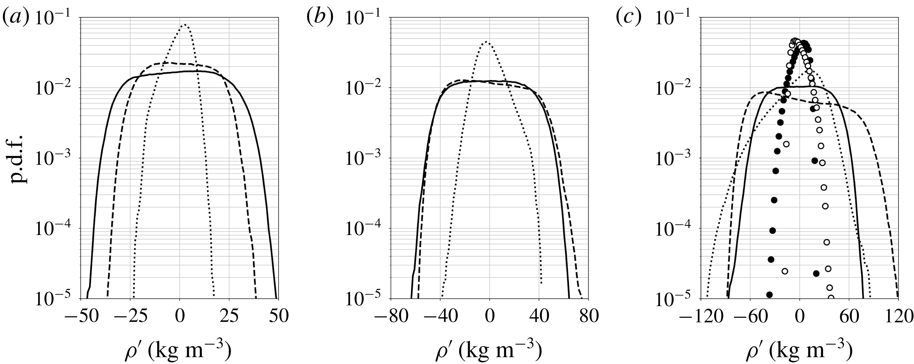
Figure 17. The p.d.f. of fluctuating density at the bottom (——, ●) and top (- - -, ○) locations of peak
 $\unicode[STIX]{x1D70C}_{rms}$
and at the average location of pseudotransition
$\unicode[STIX]{x1D70C}_{rms}$
and at the average location of pseudotransition
 $y=y_{pb}$
(
$y=y_{pb}$
(
 $\cdots \cdots$
) for
$\cdots \cdots$
) for
 $p_{b}=1.1p_{cr}$
and
$p_{b}=1.1p_{cr}$
and
 $\unicode[STIX]{x0394}T=5$
K (a), 10 K (b) and 20 K (c) and reference data for
$\unicode[STIX]{x0394}T=5$
K (a), 10 K (b) and 20 K (c) and reference data for
 $p_{b}=2p_{cr}$
and
$p_{b}=2p_{cr}$
and
 $\unicode[STIX]{x0394}T=20$
K (circles) (see § 2.3).
$\unicode[STIX]{x0394}T=20$
K (circles) (see § 2.3).

Figure 18. The p.d.f. of fluctuating temperature at the bottom (——, ●) and top (- - -, ○) locations of peak
 $T_{rms}$
and at the average location of pseudotransition
$T_{rms}$
and at the average location of pseudotransition
 $y=y_{pb}$
(
$y=y_{pb}$
(
 $\cdots \cdots$
) for
$\cdots \cdots$
) for
 $p_{b}=1.1p_{cr}$
and
$p_{b}=1.1p_{cr}$
and
 $\unicode[STIX]{x0394}T=5$
K (a), 10 K (b) and 20 K (c) and reference data for
$\unicode[STIX]{x0394}T=5$
K (a), 10 K (b) and 20 K (c) and reference data for
 $p_{b}=2p_{cr}$
and
$p_{b}=2p_{cr}$
and
 $\unicode[STIX]{x0394}T=20$
K (circles) (see § 2.3).
$\unicode[STIX]{x0394}T=20$
K (circles) (see § 2.3).
Table 7. Minimum and maximum values of fluctuating density and temperature at the approximate bottom wall (
 $y\simeq -0.97h$
) and top wall (
$y\simeq -0.97h$
) and top wall (
 $y\simeq 0.97h$
) root-mean-square peak locations and at the average location of pseudotransition,
$y\simeq 0.97h$
) root-mean-square peak locations and at the average location of pseudotransition,
 $y=y_{pb}$
.
$y=y_{pb}$
.

To gain more insight into the structure of thermodynamic fluctuations, p.d.f.s of density and temperature have been extracted at all locations (figures 15 and 16). Confirming the previous observations that the p.d.f.s widen as
 $\unicode[STIX]{x0394}T$
increases as expected, the largest variance is observed when pseudotransition takes place in the turbulent buffer layer, occurring at the top-wall buffer layer for
$\unicode[STIX]{x0394}T$
increases as expected, the largest variance is observed when pseudotransition takes place in the turbulent buffer layer, occurring at the top-wall buffer layer for
 $\unicode[STIX]{x0394}T=20$
K. While the variance of the turbulent velocity fluctuations decreases with increasing
$\unicode[STIX]{x0394}T=20$
K. While the variance of the turbulent velocity fluctuations decreases with increasing
 $\unicode[STIX]{x0394}T$
, the broader p.d.f. of thermodynamic fluctuations is associated with the steepening of the corresponding gradients (figure 6).
$\unicode[STIX]{x0394}T$
, the broader p.d.f. of thermodynamic fluctuations is associated with the steepening of the corresponding gradients (figure 6).
The analysis in figures 17 and 18 focuses on three locations, the two buffer layers and the pseudophase transitioning location, and includes a comparison with the reference data. For both density and temperature, it is observed that the pseudophase transitioning region exhibits much narrower distribution of the p.d.f.s, whereas the buffer layers display a very pronounced kurtosis. Such p.d.f. with very high kurtosis is not observed in the density p.d.f. of the reference case, while it is observed for the temperature p.d.f. (see table 7 for details).

Figure 19. The p.d.f. of
 $y/h$
values conditional to
$y/h$
values conditional to
 $|\unicode[STIX]{x1D70C}-\unicode[STIX]{x1D70C}_{pb}|\leqslant 5.9~\text{kg}~\text{m}^{-3}$
, where
$|\unicode[STIX]{x1D70C}-\unicode[STIX]{x1D70C}_{pb}|\leqslant 5.9~\text{kg}~\text{m}^{-3}$
, where
 $\unicode[STIX]{x1D70C}_{pb}=453.5~\text{kg}~\text{m}^{-3}$
, corresponding to
$\unicode[STIX]{x1D70C}_{pb}=453.5~\text{kg}~\text{m}^{-3}$
, corresponding to
 $T_{pb}\pm 0.1$
K (a) and
$T_{pb}\pm 0.1$
K (a) and
 $Q=2.49\times 10^{9}$
–
$Q=2.49\times 10^{9}$
–
 $2.51\times 10^{9}~\text{s}^{-2}$
(b) with average locations of the pseudotransition for
$2.51\times 10^{9}~\text{s}^{-2}$
(b) with average locations of the pseudotransition for
 $p_{b}=1.1p_{cr}$
and
$p_{b}=1.1p_{cr}$
and
 $\unicode[STIX]{x0394}T=5$
K (——, ○), 10 K (- - -, ▵) and 20 K (
$\unicode[STIX]{x0394}T=5$
K (——, ○), 10 K (- - -, ▵) and 20 K (
 $\cdots \cdots$
, ▫).
$\cdots \cdots$
, ▫).

Figure 20. Isosurfaces of Q-criterion at
 $Q=2.5\times 10^{9}~\text{s}^{-2}$
(a) and
$Q=2.5\times 10^{9}~\text{s}^{-2}$
(a) and
 $0.5\times 10^{9}~\text{s}^{-2}$
(b) coloured by the wall-normal velocity for
$0.5\times 10^{9}~\text{s}^{-2}$
(b) coloured by the wall-normal velocity for
 $p_{b}=1.1p_{cr}$
and
$p_{b}=1.1p_{cr}$
and
 $\unicode[STIX]{x0394}T=20$
K.
$\unicode[STIX]{x0394}T=20$
K.
Figure 19(a) presents the p.d.f. conditioned to a density range centred about its pseudotransitioning value. These results provide the probability of an instantaneous pseudophase change event at a given
 $y$
location (or equivalently, the probability of the pseudointerface being instantaneously located at a given
$y$
location (or equivalently, the probability of the pseudointerface being instantaneously located at a given
 $y$
location). The location corresponding to the highest event count moves upwards in the channel as
$y$
location). The location corresponding to the highest event count moves upwards in the channel as
 $\unicode[STIX]{x0394}T$
increases and the distribution is narrowed:
$\unicode[STIX]{x0394}T$
increases and the distribution is narrowed:
 $y/h=-0.17$
for
$y/h=-0.17$
for
 $\unicode[STIX]{x0394}T=5$
K, 0.78 for
$\unicode[STIX]{x0394}T=5$
K, 0.78 for
 $\unicode[STIX]{x0394}T=10$
K and 0.93 for
$\unicode[STIX]{x0394}T=10$
K and 0.93 for
 $\unicode[STIX]{x0394}T=20$
K. However, these values do not exactly match the average pseudotransition locations determined by the mean quantities (shown in figure 4 and indicated with symbols in figure 19), especially for
$\unicode[STIX]{x0394}T=20$
K. However, these values do not exactly match the average pseudotransition locations determined by the mean quantities (shown in figure 4 and indicated with symbols in figure 19), especially for
 $\unicode[STIX]{x0394}T=10$
K. As a result, despite having a mean pseudotransition location at
$\unicode[STIX]{x0394}T=10$
K. As a result, despite having a mean pseudotransition location at
 $y_{pb}/h=0.55$
in the
$y_{pb}/h=0.55$
in the
 $\unicode[STIX]{x0394}T=10$
K case, the greatest probability is much closer to the top wall, at about
$\unicode[STIX]{x0394}T=10$
K case, the greatest probability is much closer to the top wall, at about
 $y/h=0.8{-}0.9$
.
$y/h=0.8{-}0.9$
.
A coherent-structure-based probability distribution is also extracted (figure 19
b). Conditioning the p.d.f. on a selected Q-criteria value (
 $Q=2.49\times 10^{9}$
–
$Q=2.49\times 10^{9}$
–
 $2.51\times 10^{9}~\text{s}^{-2}$
as used in figures 20
a and 23
b) allows one to identify the effects of increasing
$2.51\times 10^{9}~\text{s}^{-2}$
as used in figures 20
a and 23
b) allows one to identify the effects of increasing
 $\unicode[STIX]{x0394}T$
on the structural make-up of turbulence under transcritical temperature conditions. In line with the observed turbulence damping in the vicinity of pseudotransition conditions, a reduction of the population density of turbulent structures in the top half of the channel is observed with increasing
$\unicode[STIX]{x0394}T$
on the structural make-up of turbulence under transcritical temperature conditions. In line with the observed turbulence damping in the vicinity of pseudotransition conditions, a reduction of the population density of turbulent structures in the top half of the channel is observed with increasing
 $\unicode[STIX]{x0394}T$
as quantitatively shown by the reduction in the number of observed events in the conditional statistics in figure 19(b). This effect is observed for several values of the Q-criterion (figure 20) and is consistent with the increasing asymmetry in the turbulent velocity profiles for increasing
$\unicode[STIX]{x0394}T$
as quantitatively shown by the reduction in the number of observed events in the conditional statistics in figure 19(b). This effect is observed for several values of the Q-criterion (figure 20) and is consistent with the increasing asymmetry in the turbulent velocity profiles for increasing
 $\unicode[STIX]{x0394}T$
as shown in figure 9.
$\unicode[STIX]{x0394}T$
as shown in figure 9.

Figure 21. One-dimensional energy spectra of Reynolds-averaged fluctuating density (a,b), wall-normal velocity (c,d) and temperature (e,f) and one-dimensional co-spectra between the Reynolds-averaged fluctuating wall-normal velocity and temperature (g,h) in the streamwise (a,c,e,g) and spanwise (b,d,f,h) direction extracted at the two near-wall peaks of density fluctuation intensity (
 $y/h=\pm 0.97$
) for
$y/h=\pm 0.97$
) for
 $p_{b}=1.1p_{cr}$
and
$p_{b}=1.1p_{cr}$
and
 $\unicode[STIX]{x0394}T=5$
K (——), 10 K (- - -) and 20 K (
$\unicode[STIX]{x0394}T=5$
K (——), 10 K (- - -) and 20 K (
 $\cdots \cdots$
). Spectra for the top-wall data have been shifted vertically by two decades for clarity.
$\cdots \cdots$
). Spectra for the top-wall data have been shifted vertically by two decades for clarity.

Figure 22. One-dimensional coherence between the Reynolds-averaged fluctuating wall-normal velocity and temperature in the streamwise (a) and spanwise (b) direction extracted at the two near-wall peaks of density fluctuation intensity (
 $y/h=\pm 0.97$
) and the average location of the pseudotransition based on the mean quantities for
$y/h=\pm 0.97$
) and the average location of the pseudotransition based on the mean quantities for
 $p_{b}=1.1p_{cr}$
and
$p_{b}=1.1p_{cr}$
and
 $\unicode[STIX]{x0394}T=5$
K (——), 10 K (- - -) and 20 K (
$\unicode[STIX]{x0394}T=5$
K (——), 10 K (- - -) and 20 K (
 $\cdots \cdots$
). Coherence for the pseudotransition and the top near-wall peak data have been shifted vertically by 0.5 and 1.0, respectively, for clarity.
$\cdots \cdots$
). Coherence for the pseudotransition and the top near-wall peak data have been shifted vertically by 0.5 and 1.0, respectively, for clarity.
Figure 21 shows one-dimensional energy spectra of fluctuating density, wall-normal velocity and temperature in the near-wall regions which are heavily affected by the wall-generated turbulence. All the profiles roll off rapidly at high wavenumbers, providing further evidence of the adequacy of the resolution of both the hydrodynamic and thermodynamic quantities (see appendix B for grid convergence study which presents a systematic sensitivity analysis of investigated simulations to the grid resolution for
 $\unicode[STIX]{x0394}T=20$
K exhibiting the strongest turbulent fluctuation). The co-spectrum of the wall-normal velocity and temperature fluctuations,
$\unicode[STIX]{x0394}T=20$
K exhibiting the strongest turbulent fluctuation). The co-spectrum of the wall-normal velocity and temperature fluctuations,
 $E_{vT}$
, is also analysed here to gain insight into the fundamental nature of their interaction. Its value increases with
$E_{vT}$
, is also analysed here to gain insight into the fundamental nature of their interaction. Its value increases with
 $\unicode[STIX]{x0394}T$
, as expected, meaning an increase of the wall-to-wall heat flux. Normalizing the co-spectrum based on the single-variable spectra (figure 22) reveals an unexpected loss of transport efficiency, or coherence, at the pseudophase changing location for intermediate wavenumbers as
$\unicode[STIX]{x0394}T$
, as expected, meaning an increase of the wall-to-wall heat flux. Normalizing the co-spectrum based on the single-variable spectra (figure 22) reveals an unexpected loss of transport efficiency, or coherence, at the pseudophase changing location for intermediate wavenumbers as
 $\unicode[STIX]{x0394}T$
is increased; this is observed for both the streamwise and spanwise directions. Overall, the hydrodynamic and thermodynamic effects are highly correlated at or around the energy-containing turbulent length scale.
$\unicode[STIX]{x0394}T$
is increased; this is observed for both the streamwise and spanwise directions. Overall, the hydrodynamic and thermodynamic effects are highly correlated at or around the energy-containing turbulent length scale.
5 Coherent structures and thermodynamics

Figure 23. Isosurfaces of density (
 $\unicode[STIX]{x1D70C}=468~\text{kg}~\text{m}^{-3}$
) coloured by the distance from the bottom wall (a), Q-criterion (
$\unicode[STIX]{x1D70C}=468~\text{kg}~\text{m}^{-3}$
) coloured by the distance from the bottom wall (a), Q-criterion (
 $Q=2.5\times 10^{9}~\text{s}^{-2}$
) coloured by the wall-normal velocity (b) and temperature gradient (c) for
$Q=2.5\times 10^{9}~\text{s}^{-2}$
) coloured by the wall-normal velocity (b) and temperature gradient (c) for
 $p_{b}=1.1p_{cr}$
and
$p_{b}=1.1p_{cr}$
and
 $\unicode[STIX]{x0394}T=5$
K (enhanced online – https://www.youtube.com/embed/JqF_ZrucSqs).
$\unicode[STIX]{x0394}T=5$
K (enhanced online – https://www.youtube.com/embed/JqF_ZrucSqs).
Instantaneous isosurfaces of density and Q-criterion as well as corresponding flooded contours of temperature gradient are shown in figure 23 for the bottom wall only to investigate the coupling between heat and mass transfer effects and the role of coherent turbulent structures in the transport. The density isosurface at
 $\unicode[STIX]{x1D70C}=468~\text{kg}~\text{m}^{-3}$
(value which corresponds to
$\unicode[STIX]{x1D70C}=468~\text{kg}~\text{m}^{-3}$
(value which corresponds to
 $y/h=-0.9$
in the mean density profile shown in figure 4) exhibits clear ejection events from the pseudoliquid region (near the cold bottom wall) as the near-wall turbulence lifts up the dense fluid into the lighter core of the channel. As the ejected fluid has more inertia than its lighter surrounding (note that no gravitational effects are accounted for in these simulations), it reaches the core of the channel where the fluid undergoes a pseudophase change, effectively achieving mass transport. Naturally, the gravitational forces (in a stably stratified flow set-up) would play a mitigating role in the observed mixing dynamics. This pseudophase change and the concomitant effects on the thermodynamics are a unique characteristic of transcritical flows and explain the high positive values of skewness of density (figure 14) in the bottom half of the channel.
$y/h=-0.9$
in the mean density profile shown in figure 4) exhibits clear ejection events from the pseudoliquid region (near the cold bottom wall) as the near-wall turbulence lifts up the dense fluid into the lighter core of the channel. As the ejected fluid has more inertia than its lighter surrounding (note that no gravitational effects are accounted for in these simulations), it reaches the core of the channel where the fluid undergoes a pseudophase change, effectively achieving mass transport. Naturally, the gravitational forces (in a stably stratified flow set-up) would play a mitigating role in the observed mixing dynamics. This pseudophase change and the concomitant effects on the thermodynamics are a unique characteristic of transcritical flows and explain the high positive values of skewness of density (figure 14) in the bottom half of the channel.
The Q-criterion isosurface identifies the turbulent structures based on the velocity gradients alone. Interestingly, large-scale streamwise-aligned structures are observed near the wall (see the circles), leading to the choice of a long computational domain length in the streamwise direction, 12 times the half-channel width, approximately twice the typical length required by the current friction Reynolds number (see table 2). Figure 23(c) shows the corresponding elongated streaks in the wall heat flux, spatially correlated with the ejection locations caused by the streamwise-elongated turbulent structures.

Figure 24. Normalized longitudinal (a,b) and lateral (c,d) two-point correlations of velocity in the streamwise (a,c) and spanwise (b,d) direction extracted at
 $y/h=-0.97$
,
$y/h=-0.97$
,
 $-$
0.75,
$-$
0.75,
 $-$
0.50,
$-$
0.50,
 $-$
0.25, 0.00, 0.25, 0.50, 0.75 and 0.97 for
$-$
0.25, 0.00, 0.25, 0.50, 0.75 and 0.97 for
 $p_{b}=1.1p_{cr}$
and
$p_{b}=1.1p_{cr}$
and
 $\unicode[STIX]{x0394}T=5$
K (——), 10 K (- - -) and 20 K (
$\unicode[STIX]{x0394}T=5$
K (——), 10 K (- - -) and 20 K (
 $\cdots \cdots$
). The lines have been shifted vertically corresponding to each
$\cdots \cdots$
). The lines have been shifted vertically corresponding to each
 $y/h$
from bottom to top. Average location of first zero-crossing points for
$y/h$
from bottom to top. Average location of first zero-crossing points for
 $\unicode[STIX]{x0394}T=5$
, 10 and 20 K (●).
$\unicode[STIX]{x0394}T=5$
, 10 and 20 K (●).
Two-point velocity correlations in the streamwise and spanwise direction (figure 24) are extracted to confirm that the computational box size has been adequately picked. A large streamwise and small spanwise coherence is observed near the top and bottom wall confirming the visual observation of the narrow elongated streaks from figure 23. We note a much longer streamwise correlation length in the
 $u$
velocity (correlation reaches zero at about
$u$
velocity (correlation reaches zero at about
 $0.15r_{x}/L_{x}$
) than in
$0.15r_{x}/L_{x}$
) than in
 $w$
(correlation reaches zero at about
$w$
(correlation reaches zero at about
 $0.05r_{x}/L_{x}$
). The lateral two-point correlations are consistent with the longitudinal ones and the three-dimensional visualizations. The signature of streamwise-aligned streaks results in a short spanwise correlation length near the walls.
$0.05r_{x}/L_{x}$
). The lateral two-point correlations are consistent with the longitudinal ones and the three-dimensional visualizations. The signature of streamwise-aligned streaks results in a short spanwise correlation length near the walls.
In the centre of the channel, turbulence is nearly isotropic, a fact observed from the integral length scale analysis. The integral length scale (not shown) at the channel centre is about 9 % of the width. The integral length scales relative to the local Kolmogorov scale are presented in figure 25 revealing the remarkably extended correlation length of the near-wall structures.

Figure 25. Ratio of the integral length scale (longitudinal (a,b) and lateral (c,d)) and the local Kolmogorov scale in the streamwise (a,c) and spanwise (b,d) direction for
 $\unicode[STIX]{x0394}T=5$
K (——), 10 K (- - -) and 20 K (
$\unicode[STIX]{x0394}T=5$
K (——), 10 K (- - -) and 20 K (
 $\cdots \cdots$
).
$\cdots \cdots$
).

Figure 26. Normalized two-point correlations of density (a,b) and compressibility factor (c,d) in the streamwise (a,c) and spanwise (b,d) direction extracted at
 $y/h=-0.97$
,
$y/h=-0.97$
,
 $-$
0.75,
$-$
0.75,
 $-$
0.50,
$-$
0.50,
 $-$
0.25, 0.00, 0.25, 0.50, 0.75 and 0.97 for
$-$
0.25, 0.00, 0.25, 0.50, 0.75 and 0.97 for
 $p_{b}=1.1p_{cr}$
and
$p_{b}=1.1p_{cr}$
and
 $\unicode[STIX]{x0394}T=5$
K (——), 10 K (- - -) and 20 K (
$\unicode[STIX]{x0394}T=5$
K (——), 10 K (- - -) and 20 K (
 $\cdots \cdots$
). The lines have been shifted vertically corresponding to each
$\cdots \cdots$
). The lines have been shifted vertically corresponding to each
 $y/h$
from bottom to top. Average location of first zero-crossing points for
$y/h$
from bottom to top. Average location of first zero-crossing points for
 $\unicode[STIX]{x0394}T=5$
, 10 and 20 K (●).
$\unicode[STIX]{x0394}T=5$
, 10 and 20 K (●).
In addition to the hydrodynamic correlations, thermodynamic two-point correlations are presented in figure 26. The two-point correlations for density and compressibility factor reflect the real fluid characteristics discussed with figure 11. The correlations have an identical tendency showing the long streamwise and short spanwise correlation lengths near the walls and vice versa in the centre region. The large streamwise coherence near the walls accords with the manifestation of pseudoliquid flow streaks observed in figure 23. These longer streaky structures are also observed in variable-density, supersonic wall-bounded flows with cooled walls (Coleman, Kim & Moser Reference Coleman, Kim and Moser1995). As the fluctuating density is enhanced (see figure 13), so is the momentum transfer along the wall-normal direction. As a result, the higher momentum particles travel a longer distance, imparting an enhanced streaky structure to the near-wall flow. The flow ejected from the walls in the long streamwise streaks eventually takes on a blob-like form (shorter streamwise, longer spanwise structure) as the ejected fluid reaches the channel centreplane. The strong similarity between all
 $\unicode[STIX]{x0394}T$
conditions is noted.
$\unicode[STIX]{x0394}T$
conditions is noted.
6 Conclusions
We have performed DNS of transcritical turbulent channel flow with differentially heated walls (
 $T_{top}-T_{bot}=\unicode[STIX]{x0394}T$
) of R-134a (also called 1,1,1,2-tetrafluoroethane,
$T_{top}-T_{bot}=\unicode[STIX]{x0394}T$
) of R-134a (also called 1,1,1,2-tetrafluoroethane,
 $\text{CH}_{2}\text{FCF}_{3}$
) at a slightly supercritical pressure. By defining a statistically steady turbulent channel flow at transcritical temperature conditions, the turbulence and thermodynamic coupling could be studied. The simulations were conducted by solving the fully compressible Navier–Stokes equations using a conservative formulation. Special attention was paid to fully resolving all scales of the hydrodynamics and thermodynamics of the set-up to avoid non-physical oscillations which are characteristics of these flows. The PR EoS was used with a consistent thermodynamic formulation to investigate the real fluid effects. The simulations were run at a friction Reynolds number of about
$\text{CH}_{2}\text{FCF}_{3}$
) at a slightly supercritical pressure. By defining a statistically steady turbulent channel flow at transcritical temperature conditions, the turbulence and thermodynamic coupling could be studied. The simulations were conducted by solving the fully compressible Navier–Stokes equations using a conservative formulation. Special attention was paid to fully resolving all scales of the hydrodynamics and thermodynamics of the set-up to avoid non-physical oscillations which are characteristics of these flows. The PR EoS was used with a consistent thermodynamic formulation to investigate the real fluid effects. The simulations were run at a friction Reynolds number of about
 $Re_{\unicode[STIX]{x1D70F}}=373$
. A realistic Prandtl number is used and computed from Chung’s model to estimate the dynamic viscosity and thermal conductivity. By varying the differential heating of the channel walls, the average location of the pseudophase change could be controlled, with
$Re_{\unicode[STIX]{x1D70F}}=373$
. A realistic Prandtl number is used and computed from Chung’s model to estimate the dynamic viscosity and thermal conductivity. By varying the differential heating of the channel walls, the average location of the pseudophase change could be controlled, with
 $y/h=-0.23$
, 0.55 and 0.89 for
$y/h=-0.23$
, 0.55 and 0.89 for
 $\unicode[STIX]{x0394}T=5$
, 10 and 20 K, respectively. At the pseudophase change, the thermodynamic nonlinearities are maximal, and therefore the resulting effects of the thermodynamic nonlinearities on turbulence could be investigated.
$\unicode[STIX]{x0394}T=5$
, 10 and 20 K, respectively. At the pseudophase change, the thermodynamic nonlinearities are maximal, and therefore the resulting effects of the thermodynamic nonlinearities on turbulence could be investigated.
Conventional near-wall velocity scaling laws cannot capture the velocity distribution in transcritical flows due to the large density and thermophysical variations; even recent improvements to the scaling laws for heated and cooled walls cannot accurately capture these effects. This leads us to conclude that additional wall modelling for transcritical flow is essential to correctly capture the near-wall dynamics of transcritical flows. One justification for the near-wall modelling challenges stems from nonlinear thermodynamic effects in the wall turbulence. The real fluid thermodynamic effects inhibit hydrodynamic turbulence through a decrease in the dilatational production term of the enstrophy equation (not shown). The profiles of the thermodynamic fluctuations show a higher intensity in the pseudogas (hot wall) compared to the pseudoliquid (cold wall) region; this occurs despite a reduction in the turbulence intensity near the top wall. The conditional p.d.f. of density shows narrowing of the pseudotransition region with increasing differential heating. When the pseudophase change occurs near the wall (
 $\unicode[STIX]{x0394}T=20$
K case), a highly skewed and very narrow distribution is observed, which results from the nonlinear dynamics as the pseudophase change occurs near the viscous sublayer. The structural signature of the turbulence in transcritical flows remains the most striking. Near the wall, the turbulence is aligned in the long, yet meandering, streamwise coherent structures and the integral length scales are over 400 times the local Kolmogorov scale. The instantaneous visualizations and the two-point correlations have shown that strong ejections of heavy fluid into the channel core affect the structures and dynamics of turbulent channel flow and leave streaks in the temperature gradients at the wall.
$\unicode[STIX]{x0394}T=20$
K case), a highly skewed and very narrow distribution is observed, which results from the nonlinear dynamics as the pseudophase change occurs near the viscous sublayer. The structural signature of the turbulence in transcritical flows remains the most striking. Near the wall, the turbulence is aligned in the long, yet meandering, streamwise coherent structures and the integral length scales are over 400 times the local Kolmogorov scale. The instantaneous visualizations and the two-point correlations have shown that strong ejections of heavy fluid into the channel core affect the structures and dynamics of turbulent channel flow and leave streaks in the temperature gradients at the wall.
Acknowledgements
This work has been performed under the support of the University Technology Center (UTC) in Advanced Thermal Management Systems at Purdue University led by Mr P. Sweeney (Rolls-Royce, Indianapolis) and Professor S. D. Heister (Purdue). The authors also thank J. Larsson for providing us with the high-order structured code Hybrid. J.P.H. acknowledges the support from the Natural Sciences and Engineering Research Council of Canada (NSERC) Discovery Grants Program. The computing resources were provided by the Rosen Center for Advanced Computing (RCAC) at Purdue University and Information Technology at Purdue (ITaP) and the SciNet High-Performance Computing system which is one of the Compute/Calcul Canada consortia.
Appendix A. Modelling of thermodynamic and fluid transport properties
The PR EoS (Peng & Robinson Reference Peng and Robinson1976) reads
 $$\begin{eqnarray}\displaystyle \left.\begin{array}{@{}c@{}}\displaystyle p=\frac{R_{u}T}{v_{m}-b}-\frac{a\unicode[STIX]{x1D6FC}}{v_{m}^{2}+2bv_{m}-b^{2}},\\ \displaystyle a=\frac{0.45724R_{u}^{2}T_{cr}^{2}}{p_{cr}},\quad b=\frac{0.07780R_{u}T_{cr}}{p_{cr}},\\ \displaystyle \unicode[STIX]{x1D6FC}=[1+(0.37464+1.54226\unicode[STIX]{x1D714}-0.26992\unicode[STIX]{x1D714}^{2})(1-T_{r}^{0.5})]^{2},\end{array}\right\} & & \displaystyle\end{eqnarray}$$
where
 $R_{u}$
is the universal gas constant,
$R_{u}$
is the universal gas constant,
 $v_{m}$
the molar volume,
$v_{m}$
the molar volume,
 $\unicode[STIX]{x1D714}$
the acentric factor and
$\unicode[STIX]{x1D714}$
the acentric factor and
 $T_{r}=T/T_{cr}$
the reduced temperature. The terms,
$T_{r}=T/T_{cr}$
the reduced temperature. The terms,
 $a$
,
$a$
,
 $b$
and
$b$
and
 $\unicode[STIX]{x1D6FC}$
account for intermolecular attractive and repulsive effects and the non-spherical shape of the molecules.
$\unicode[STIX]{x1D6FC}$
account for intermolecular attractive and repulsive effects and the non-spherical shape of the molecules.
The thermodynamic relations based on the PR EoS that incorporate departure functions are
 $$\begin{eqnarray}\displaystyle & \displaystyle e(T,\unicode[STIX]{x1D70C})=e^{0}(T)+\frac{1}{\sqrt{8}bM_{w}}\left[T\left(\frac{\unicode[STIX]{x2202}a\unicode[STIX]{x1D6FC}}{\unicode[STIX]{x2202}T}\right)-a\unicode[STIX]{x1D6FC}\right]\ln \left(\frac{M_{w}+(1+\sqrt{2})b\unicode[STIX]{x1D70C}}{M_{w}+(1-\sqrt{2})b\unicode[STIX]{x1D70C}}\right), & \displaystyle\end{eqnarray}$$
 $$\begin{eqnarray}\displaystyle & \displaystyle h(T,\unicode[STIX]{x1D70C})=e(T,\unicode[STIX]{x1D70C})+\frac{p}{\unicode[STIX]{x1D70C}}, & \displaystyle\end{eqnarray}$$
 $$\begin{eqnarray}\displaystyle & \displaystyle c_{v}(T,\unicode[STIX]{x1D70C})=c_{v}^{0}(T)+\frac{T}{\sqrt{8}bM_{w}}\left(\frac{\unicode[STIX]{x2202}^{2}a\unicode[STIX]{x1D6FC}}{\unicode[STIX]{x2202}T^{2}}\right)\ln \left(\frac{M_{w}+(1+\sqrt{2})b\unicode[STIX]{x1D70C}}{M_{w}+(1-\sqrt{2})b\unicode[STIX]{x1D70C}}\right), & \displaystyle\end{eqnarray}$$
 $$\begin{eqnarray}\displaystyle & \displaystyle c_{p}(T,\unicode[STIX]{x1D70C})=c_{v}(T,\unicode[STIX]{x1D70C})+\frac{T}{\unicode[STIX]{x1D70C}^{2}}\left(\frac{\unicode[STIX]{x2202}p}{\unicode[STIX]{x2202}T}\right)_{\unicode[STIX]{x1D70C}}^{2}/\left(\frac{\unicode[STIX]{x2202}p}{\unicode[STIX]{x2202}\unicode[STIX]{x1D70C}}\right)_{T}, & \displaystyle\end{eqnarray}$$
 $$\begin{eqnarray}\displaystyle & \displaystyle \unicode[STIX]{x1D6FE}(T,\unicode[STIX]{x1D70C})=\frac{c_{p}(T,\unicode[STIX]{x1D70C})}{c_{v}(T,\unicode[STIX]{x1D70C})}, & \displaystyle\end{eqnarray}$$
 $$\begin{eqnarray}\displaystyle & \displaystyle c(T,\unicode[STIX]{x1D70C})=\sqrt{\unicode[STIX]{x1D6FE}(T,\unicode[STIX]{x1D70C})\left(\frac{\unicode[STIX]{x2202}p}{\unicode[STIX]{x2202}\unicode[STIX]{x1D70C}}\right)_{T}}, & \displaystyle\end{eqnarray}$$
where
 $e$
is the internal energy,
$e$
is the internal energy,
 $h$
the enthalpy,
$h$
the enthalpy,
 $c_{v}$
the heat capacity at constant volume,
$c_{v}$
the heat capacity at constant volume,
 $c_{p}$
the heat capacity at constant pressure,
$c_{p}$
the heat capacity at constant pressure,
 $\unicode[STIX]{x1D6FE}$
the specific heat ratio,
$\unicode[STIX]{x1D6FE}$
the specific heat ratio,
 $c$
the speed of sound and
$c$
the speed of sound and
 $M_{w}$
the molecular weight. The superscript
$M_{w}$
the molecular weight. The superscript
 $0$
denotes the thermodynamic property of the equivalent ideal gas state.
$0$
denotes the thermodynamic property of the equivalent ideal gas state.
Departure functions derived from the selected EoS ensure full thermodynamic consistency (Ewing & Peters Reference Ewing and Peters2000) of the simulations. As an example, here the partial derivatives in the relations for
 $c_{p}$
and
$c_{p}$
and
 $c$
are given by
$c$
are given by
 $$\begin{eqnarray}\displaystyle & \displaystyle \left(\frac{\unicode[STIX]{x2202}p}{\unicode[STIX]{x2202}T}\right)_{\unicode[STIX]{x1D70C}}=\frac{\unicode[STIX]{x1D70C}R_{u}}{M_{w}-b\unicode[STIX]{x1D70C}}-\left(\frac{\unicode[STIX]{x2202}a\unicode[STIX]{x1D6FC}}{\unicode[STIX]{x2202}T}\right)\frac{\unicode[STIX]{x1D70C}^{2}}{[M_{w}+(1+\sqrt{2})b\unicode[STIX]{x1D70C}][M_{w}+(1-\sqrt{2})b\unicode[STIX]{x1D70C}]}, & \displaystyle\end{eqnarray}$$
 $$\begin{eqnarray}\displaystyle & \displaystyle \left(\frac{\unicode[STIX]{x2202}p}{\unicode[STIX]{x2202}\unicode[STIX]{x1D70C}}\right)_{T}=\frac{M_{w}R_{u}T}{(M_{w}-b\unicode[STIX]{x1D70C})^{2}}-\frac{2a\unicode[STIX]{x1D6FC}\unicode[STIX]{x1D70C}M_{w}(M_{w}+b\unicode[STIX]{x1D70C})}{[M_{w}+(1+\sqrt{2})b\unicode[STIX]{x1D70C}]^{2}[M_{w}+(1-\sqrt{2})b\unicode[STIX]{x1D70C}]^{2}}. & \displaystyle\end{eqnarray}$$
Chung’s method (Chung et al. Reference Chung, Ajlan, Lee and Starling1988) is used to obtain transport properties such as dynamic viscosity and thermal conductivity. The dynamic viscosity is given by
 $$\begin{eqnarray}\displaystyle \unicode[STIX]{x1D707}=\unicode[STIX]{x1D707}^{\ast }\frac{36.344(M_{w}T_{cr})^{1/2}}{v_{m,c}^{2/3}}, & & \displaystyle\end{eqnarray}$$
where
 $v_{m,c}$
is the critical molar volume and
$v_{m,c}$
is the critical molar volume and
 $\unicode[STIX]{x1D707}^{\ast }$
is
$\unicode[STIX]{x1D707}^{\ast }$
is
 $$\begin{eqnarray}\displaystyle \unicode[STIX]{x1D707}^{\ast }=\frac{(T^{\ast })^{1/2}}{\unicode[STIX]{x1D6FA}_{v}}F_{c}[(G_{2})^{-1}+A_{6}y]+\unicode[STIX]{x1D707}^{\ast \ast }. & & \displaystyle\end{eqnarray}$$
Parameters
 $T^{\ast }$
,
$T^{\ast }$
,
 $\unicode[STIX]{x1D6FA}_{v}$
and
$\unicode[STIX]{x1D6FA}_{v}$
and
 $F_{c}$
are given as
$F_{c}$
are given as
 $$\begin{eqnarray}\displaystyle & \displaystyle T^{\ast }=1.2593T_{r}, & \displaystyle\end{eqnarray}$$
 $$\begin{eqnarray}\displaystyle & \displaystyle \unicode[STIX]{x1D6FA}_{v}=[A(T^{\ast })^{-B}]+C[\exp (-DT^{\ast })]+E[\exp (-FT^{\ast })]+GT^{\ast B}\sin (ST^{\ast W}-H), & \displaystyle\end{eqnarray}$$
 $$\begin{eqnarray}\displaystyle & \displaystyle F_{c}=1-0.2756\unicode[STIX]{x1D714}+0.059035\unicode[STIX]{x1D707}_{r}^{4}+\unicode[STIX]{x1D705}_{a}, & \displaystyle\end{eqnarray}$$
where
 $\unicode[STIX]{x1D705}_{a}$
is the association factor for hydrogen bonding effect of highly polar substances such as alcohols and acids and
$\unicode[STIX]{x1D705}_{a}$
is the association factor for hydrogen bonding effect of highly polar substances such as alcohols and acids and
 $\unicode[STIX]{x1D6FA}_{v}$
and
$\unicode[STIX]{x1D6FA}_{v}$
and
 $F_{c}$
mean the viscosity collision integral and consideration for the shape and the polarity of molecules for dilute gases, respectively. The dimensionless dipole moment,
$F_{c}$
mean the viscosity collision integral and consideration for the shape and the polarity of molecules for dilute gases, respectively. The dimensionless dipole moment,
 $\unicode[STIX]{x1D707}_{r}$
, is given by
$\unicode[STIX]{x1D707}_{r}$
, is given by
 $$\begin{eqnarray}\displaystyle \unicode[STIX]{x1D707}_{r}=131.3\frac{\unicode[STIX]{x1D712}}{(v_{m,c}T_{cr})^{1/2}}, & & \displaystyle\end{eqnarray}$$
where
 $\unicode[STIX]{x1D712}$
is the dipole moment of molecules.
$\unicode[STIX]{x1D712}$
is the dipole moment of molecules.

Figure 27. Thermodynamic properties predicted by the PR EoS and Chung’s model (lines) and the NIST data (symbols) at various pressure conditions (—— ○,
 $p_{cr}=40.590$
bar; - - - ▵,
$p_{cr}=40.590$
bar; - - - ▵,
 $1.1p_{cr}=44.649$
bar; — ⋅ — ▫,
$1.1p_{cr}=44.649$
bar; — ⋅ — ▫,
 $1.2p_{cr}=48.708$
bar; ●,
$1.2p_{cr}=48.708$
bar; ●,
 $2p_{cr}=81.180$
bar). (a) Density (●, critical point). (b) Speed of sound. (c) Heat capacity at constant volume. (d) Heat capacity at constant pressure. (e) Internal energy. (f) Enthalpy. (g) Dynamic viscosity. (h) Thermal conductivity. (i) Specific heat ratio. (j) Prandtl number.
$2p_{cr}=81.180$
bar). (a) Density (●, critical point). (b) Speed of sound. (c) Heat capacity at constant volume. (d) Heat capacity at constant pressure. (e) Internal energy. (f) Enthalpy. (g) Dynamic viscosity. (h) Thermal conductivity. (i) Specific heat ratio. (j) Prandtl number.
The other terms appearing in the relationships above are as follows:
 $$\begin{eqnarray}\displaystyle & \displaystyle y=\frac{\unicode[STIX]{x1D70C}v_{m,c}}{6}, & \displaystyle\end{eqnarray}$$
 $$\begin{eqnarray}\displaystyle & \displaystyle G_{1}=\frac{1-0.5y}{(1-y)^{3}}, & \displaystyle\end{eqnarray}$$
 $$\begin{eqnarray}\displaystyle & \displaystyle G_{2}=\frac{A_{1}[[1-\exp (-A_{4}y)]/y]+A_{2}G_{1}\exp (A_{5}y)+A_{3}G_{1}}{A_{1}A_{4}+A_{2}+A_{3}}, & \displaystyle\end{eqnarray}$$
 $$\begin{eqnarray}\displaystyle & \displaystyle \unicode[STIX]{x1D707}^{\ast \ast }=A_{7}y^{2}G_{2}\exp [A_{8}+A_{9}(T^{\ast })^{-1}+A_{10}(T^{\ast })^{-2}], & \displaystyle\end{eqnarray}$$
 $$\begin{eqnarray}\displaystyle & \displaystyle A_{i}=a_{0}(i)+a_{1}(i)\unicode[STIX]{x1D714}+a_{2}(i)\unicode[STIX]{x1D707}_{r}^{4}+a_{3}(i)\unicode[STIX]{x1D705}_{a}. & \displaystyle\end{eqnarray}$$
The thermal conductivity was developed by following a similar approach to the dynamic viscosity:
 $$\begin{eqnarray}\displaystyle \unicode[STIX]{x1D706}=\frac{31.2\unicode[STIX]{x1D707}^{0}\unicode[STIX]{x1D6F9}}{M_{w}^{\prime }}(G_{2}^{-1}+B_{6}y)+qB_{7}y^{2}T_{r}^{1/2}G_{2}, & & \displaystyle\end{eqnarray}$$
where
 $$\begin{eqnarray}\displaystyle & \displaystyle \unicode[STIX]{x1D707}^{0}=40.785\frac{F_{c}(M_{w}T)^{1/2}}{v_{m,c}^{2/3}\unicode[STIX]{x1D6FA}_{v}}, & \displaystyle\end{eqnarray}$$
 $$\begin{eqnarray}\displaystyle & \displaystyle \unicode[STIX]{x1D6F9}=1+\unicode[STIX]{x1D6FC}\left(\frac{0.215+0.28288\unicode[STIX]{x1D6FC}-1.061\unicode[STIX]{x1D6FD}+0.26665Z}{0.6366+\unicode[STIX]{x1D6FD}Z+1.061\unicode[STIX]{x1D6FC}\unicode[STIX]{x1D6FD}}\right), & \displaystyle\end{eqnarray}$$
 $$\begin{eqnarray}\displaystyle & \displaystyle \unicode[STIX]{x1D6FC}=\frac{c_{v}}{R_{u}}-1.5, & \displaystyle\end{eqnarray}$$
 $$\begin{eqnarray}\displaystyle & \displaystyle \unicode[STIX]{x1D6FD}=0.7862-0.7109\unicode[STIX]{x1D714}+1.3168\unicode[STIX]{x1D714}^{2}, & \displaystyle\end{eqnarray}$$
 $$\begin{eqnarray}\displaystyle & \displaystyle Z=2.0+10.5T_{r}^{2}, & \displaystyle\end{eqnarray}$$
 $$\begin{eqnarray}\displaystyle & \displaystyle M_{w}^{\prime }=M_{w}/10^{3}, & \displaystyle\end{eqnarray}$$
 $$\begin{eqnarray}\displaystyle & \displaystyle q=3.586\times 10^{-3}\frac{(T_{cr}/M_{w}^{\prime })^{1/2}}{v_{m,c}^{2/3}}. & \displaystyle\end{eqnarray}$$
For the term
 $G_{2}$
, the form is identical to that of dynamic viscosity, but
$G_{2}$
, the form is identical to that of dynamic viscosity, but
 $A_{i}$
is replaced with
$A_{i}$
is replaced with
 $B_{i}$
which has different values. All the other terms that are not defined here and the empirical coefficients are found in Poling et al. (Reference Poling, Prausnitz and O’Connell2001).
$B_{i}$
which has different values. All the other terms that are not defined here and the empirical coefficients are found in Poling et al. (Reference Poling, Prausnitz and O’Connell2001).
Appendix B. Grid convergence study

Figure 28. Root-mean-square of streamwise (a), wall-normal (b) and spanwise (c) Favre fluctuating velocity component and Reynolds shear stress (d) for
 $p_{b}=1.1p_{cr}$
and
$p_{b}=1.1p_{cr}$
and
 $\unicode[STIX]{x0394}T=20$
K at grid resolution of
$\unicode[STIX]{x0394}T=20$
K at grid resolution of
 $64\times 96\times 64$
(
$64\times 96\times 64$
(
 $\cdots \cdots$
),
$\cdots \cdots$
),
 $128\times 128\times 96$
(— ⋅ —),
$128\times 128\times 96$
(— ⋅ —),
 $192\times 128\times 128$
(- - -),
$192\times 128\times 128$
(- - -),
 $384\times 256\times 256$
(– –) and
$384\times 256\times 256$
(– –) and
 $512\times 256\times 256$
(——).
$512\times 256\times 256$
(——).
Table 8. Filtering factors used in the top-hat filter.


Figure 29. Root-mean-square of Reynolds fluctuations for density (a), temperature (b) and pressure (c) for
 $p_{b}=1.1p_{cr}$
and
$p_{b}=1.1p_{cr}$
and
 $\unicode[STIX]{x0394}T=20$
K at grid resolution of
$\unicode[STIX]{x0394}T=20$
K at grid resolution of
 $64\times 96\times 64$
(
$64\times 96\times 64$
(
 $\cdots \cdots$
),
$\cdots \cdots$
),
 $128\times 128\times 96$
(— ⋅ —),
$128\times 128\times 96$
(— ⋅ —),
 $192\times 128\times 128$
(- - -),
$192\times 128\times 128$
(- - -),
 $384\times 256\times 256$
(– –) and
$384\times 256\times 256$
(– –) and
 $512\times 256\times 256$
(——).
$512\times 256\times 256$
(——).

Figure 30. Root-mean-square of Favre fluctuations for enthalpy (a) and wall-normal turbulent enthalpy flux (b) for
 $p_{b}=1.1p_{cr}$
and
$p_{b}=1.1p_{cr}$
and
 $\unicode[STIX]{x0394}T=20$
K at grid resolution of
$\unicode[STIX]{x0394}T=20$
K at grid resolution of
 $64\times 96\times 64$
(
$64\times 96\times 64$
(
 $\cdots \cdots$
),
$\cdots \cdots$
),
 $128\times 128\times 96$
(— ⋅ —),
$128\times 128\times 96$
(— ⋅ —),
 $192\times 128\times 128$
(- - -),
$192\times 128\times 128$
(- - -),
 $384\times 256\times 256$
(– –) and
$384\times 256\times 256$
(– –) and
 $512\times 256\times 256$
(——).
$512\times 256\times 256$
(——).
Grid convergence of transcritical flows is essential for determining the adequacy of DNS as we recall that the minimal thermodynamic length scale to be resolved in transcritical flows is typically smaller than the Kolmogorov length scale. Insufficient spatial resolution is typically evidenced by a large spectral pile-up in the thermodynamic quantities; in which case, the obtained results should be considered erroneous. In order to resolve the numerical error, we have used the top-hat filter with filtering factors shown in table 8. Here, the grid sensitivity is investigated for the most critical case of
 $\unicode[STIX]{x0394}T=20$
K. Figure 28 shows the grid sensitivity of the velocity root-mean-square. We highlight the insensitivity of the streamwise fluctuations to the grid resolution, whereas an unresolved simulation underestimates the peak fluctuations in the spanwise and wall-normal velocity components. The overall trends of the root-mean-square profiles (asymmetry, relative peak height, etc.) are independent of the grid resolution.
$\unicode[STIX]{x0394}T=20$
K. Figure 28 shows the grid sensitivity of the velocity root-mean-square. We highlight the insensitivity of the streamwise fluctuations to the grid resolution, whereas an unresolved simulation underestimates the peak fluctuations in the spanwise and wall-normal velocity components. The overall trends of the root-mean-square profiles (asymmetry, relative peak height, etc.) are independent of the grid resolution.
The grid sensitivity of thermodynamic fluctuations is shown in figures 29 and 30. We note a slow convergence of the thermodynamic quantities, particularly for the pressure. Figure 30 shows that the fluctuating enthalpy root-mean-square is well captured on a coarse mesh. However, the turbulent enthalpy flux, an important quantity for the characterization of the convective heat transfer, requires a large grid count for a correct estimation. An insufficient grid resolution will underestimate the magnitude of the turbulent effect on the heat transfer in this transcritical system.

Figure 31. One-dimensional energy spectra of Reynolds-averaged fluctuating density (a,b), wall-normal velocity (c,d) and temperature (e,f) in the streamwise (a,c,e) and spanwise (b,d,f) directions extracted at the two near-wall peaks of density fluctuation intensity (
 $y/h=\pm 0.97$
) and the centreplane (
$y/h=\pm 0.97$
) and the centreplane (
 $y/h=0$
) for
$y/h=0$
) for
 $p_{b}=1.1p_{cr}$
and
$p_{b}=1.1p_{cr}$
and
 $\unicode[STIX]{x0394}T=20$
K at grid resolution of
$\unicode[STIX]{x0394}T=20$
K at grid resolution of
 $64\times 96\times 64$
(
$64\times 96\times 64$
(
 $\cdots \cdots$
),
$\cdots \cdots$
),
 $128\times 128\times 96$
(— ⋅ —),
$128\times 128\times 96$
(— ⋅ —),
 $192\times 128\times 128$
(- - -),
$192\times 128\times 128$
(- - -),
 $384\times 256\times 256$
(– –) and
$384\times 256\times 256$
(– –) and
 $512\times 256\times 256$
(——). Spectra for the centreplane and the top-wall data have been shifted vertically by three decades and six decades, respectively, for clarity.
$512\times 256\times 256$
(——). Spectra for the centreplane and the top-wall data have been shifted vertically by three decades and six decades, respectively, for clarity.
The one-dimensional energy spectra of fluctuating density, wall-normal velocity and temperature in the streamwise and spanwise directions are presented in figure 31. The profiles are extracted at
 $y/h=-0.97$
, 0 and 0.97 which correspond to the location of the thermodynamic root-mean-square peaks (bottom and top wall) and the centreplane. As the grid resolution increases, a spectral broadening is observed with a slight increase at the high wavenumbers. Also, a build-up at high wavenumbers in the energy spectra is observed as expected because of the higher sensitivity to inadequate spatial resolution due to the coupling of conservative compressible methods with cubic equations of state. The latter were mitigated by adopting a higher numerical resolution than that normally required for the given Reynolds number.
$y/h=-0.97$
, 0 and 0.97 which correspond to the location of the thermodynamic root-mean-square peaks (bottom and top wall) and the centreplane. As the grid resolution increases, a spectral broadening is observed with a slight increase at the high wavenumbers. Also, a build-up at high wavenumbers in the energy spectra is observed as expected because of the higher sensitivity to inadequate spatial resolution due to the coupling of conservative compressible methods with cubic equations of state. The latter were mitigated by adopting a higher numerical resolution than that normally required for the given Reynolds number.

Figure 32. Normalized average Kolmogorov length scales
 $\overline{\unicode[STIX]{x1D702}}_{K}/\unicode[STIX]{x0394}x$
(a),
$\overline{\unicode[STIX]{x1D702}}_{K}/\unicode[STIX]{x0394}x$
(a),
 $\overline{\unicode[STIX]{x1D702}}_{K}/\unicode[STIX]{x0394}y$
(b) and
$\overline{\unicode[STIX]{x1D702}}_{K}/\unicode[STIX]{x0394}y$
(b) and
 $\overline{\unicode[STIX]{x1D702}}_{K}/\unicode[STIX]{x0394}z$
(c), at
$\overline{\unicode[STIX]{x1D702}}_{K}/\unicode[STIX]{x0394}z$
(c), at
 $p_{b}=1.1p_{cr}$
and
$p_{b}=1.1p_{cr}$
and
 $\unicode[STIX]{x0394}T=20$
K at grid resolution of
$\unicode[STIX]{x0394}T=20$
K at grid resolution of
 $64\times 96\times 64$
(
$64\times 96\times 64$
(
 $\cdots \cdots$
),
$\cdots \cdots$
),
 $128\times 128\times 96$
(
$128\times 128\times 96$
(
 $\text{-}\cdot \text{-}$
),
$\text{-}\cdot \text{-}$
),
 $192\times 128\times 128$
(- - -),
$192\times 128\times 128$
(- - -),
 $384\times 256\times 256$
(– –) and
$384\times 256\times 256$
(– –) and
 $512\times 256\times 256$
(——).
$512\times 256\times 256$
(——).
Figure 32 presents the average profiles of the normalized Kolmogorov length scale in the streamwise, wall-normal and spanwise directions. The Kolmogorov scale,
 $\unicode[STIX]{x1D702}_{K}$
, which quantifies the smallest turbulence length scale, is defined as
$\unicode[STIX]{x1D702}_{K}$
, which quantifies the smallest turbulence length scale, is defined as
 $$\begin{eqnarray}\displaystyle \unicode[STIX]{x1D702}_{K}\equiv \left(\frac{\unicode[STIX]{x1D708}^{3}}{\unicode[STIX]{x1D716}}\right)^{1/4}, & & \displaystyle\end{eqnarray}$$
where
 $\unicode[STIX]{x1D708}$
and
$\unicode[STIX]{x1D708}$
and
 $\unicode[STIX]{x1D716}$
represent the kinematic viscosity and dissipation rate of turbulent kinetic energy per unit mass. For compressible flows,
$\unicode[STIX]{x1D716}$
represent the kinematic viscosity and dissipation rate of turbulent kinetic energy per unit mass. For compressible flows,
 $\unicode[STIX]{x1D716}$
reads
$\unicode[STIX]{x1D716}$
reads
 $$\begin{eqnarray}\displaystyle \unicode[STIX]{x1D716}\equiv \frac{1}{\overline{\unicode[STIX]{x1D70C}}}\overline{\unicode[STIX]{x1D70F}_{ij}\frac{\unicode[STIX]{x2202}u_{i}^{\prime \prime }}{\unicode[STIX]{x2202}x_{j}}}. & & \displaystyle\end{eqnarray}$$
The profiles of the normalized Kolmogorov length scale approach unity as the grid resolution increases. It is observed that the flow in the liquid-like phase needs a finer grid than that in the gas-like phase to resolve the turbulence length scale. These figures show adequate grid resolution in the wall-normal direction, especially near the walls. This study highlights the importance of a sufficient resolution in the streamwise direction as well.