


1. Introduction
Controlled manipulation of small particles in suspension is crucial in fundamental research and applications such as biomedical and biochemical processing (Ateya et al. Reference Ateya, Erickson, Howell, Hilliard, Golden and Ligler2008; Nilsson et al. Reference Nilsson, Evander, Hammarström and Laurell2009), disease diagnostics and therapeutics (Gossett et al. Reference Gossett, Weaver, Mach, Hur, Tse, Lee, Amini and Di Carlo2010; Puri & Ganguly Reference Puri and Ganguly2014), drug discovery and delivery systems (Dittrich & Manz Reference Dittrich and Manz2006; Nguyen et al. Reference Nguyen, Shaegh, Kashaninejad and Phan2013), self-cleaning and antifouling technologies (Callow & Callow Reference Callow and Callow2011; Kirschner & Brennan Reference Kirschner and Brennan2012). The essence of particle manipulation is to drive the particles across streamlines, making them follow specific pathlines (trajectories) distinct from the fluid elements based on their properties.
Microfluidic particle manipulation aims at transportation, separation, trapping and enrichment (Sajeesh & Sen Reference Sajeesh and Sen2014; Lu et al. Reference Lu, Liu, Hu and Xuan2017) and can be achieved through various approaches. Many techniques exploit certain particles’ response to external forces, e.g. electrical (Xuan Reference Xuan2019), optical (Lenshof & Laurell Reference Lenshof and Laurell2010) and magnetic (Van Reenen et al. Reference van Reenen, de Jong, den Toonder and Prins2014) techniques. However, not all particles of interest will be susceptible to these, which is why there is a continued interest in manipulation based solely on hydrodynamic forces (Karimi et al. Reference Karimi, Yazdi and Ardekani2013). Most notably, techniques that use particle inertia have gained prominence (Di Carlo et al. Reference Di Carlo, Dino, Daniel, Ronald and Toner2007; Di Carlo Reference Di Carlo2009; Agarwal et al. Reference Agarwal, Rallabandi and Hilgenfeldt2018) and quantitative theories have been developed beyond classical equations of motion (Maxey & Riley Reference Maxey and Riley1983) to rigorously describe the effect of inertial forces in both the background flow and the disturbance flow around the particle (Agarwal et al. Reference Agarwal, Chan, Rallabandi, Gazzola and Hilgenfeldt2021; Agarwal Reference Agarwal2021). Recent work by Agarwal et al. (Reference Agarwal, Upadhyay, Bhosale, Gazzola and Hilgenfeldt2024) also integrates the important case of acoustofluidic particle manipulation (Bruus et al. Reference Bruus, Dual, Hawkes, Hill, Laurell, Nilsson, Radel, Sadhal and Wiklund2011; Laurell et al. Reference Laurell, Petersson and Nilsson2007; Friend & Yeo Reference Friend and Yeo2011) as a particular limit of inertial particle manipulation. Despite the description of such forces in simple flow fields that is now known analytically, many practical cases still lack a fundamental quantitative theory on how devices based on hydrodynamic effects work.
This also applies to viscous Stokes flow. Even in the absence of inertia, particles interact hydrodynamically with other particles or large-scale interfaces (walls or fluid–fluid boundaries), with effective interactions that are notoriously long-ranged (Happel & Brenner Reference Happel and Brenner1965; Brady & Bossis Reference Brady and Bossis1988; Pozrikidis Reference Pozrikidis1992; Kim & Karrila Reference Pozrikidis2011, Reference Kim and Karrila2013). Early theoretical efforts by Brady & Bossis (Reference Brady and Bossis1988) and Claeys & Brady (Reference Claeys and Brady1989, Reference Claeys and Brady1993) show in general terms that a particle moving in a Stokes flow should never experience surface-to-surface contact with a boundary (interfaces cannot touch in finite time). However, in practical situations where Stokes flow around obstacles is used to manipulate particles, such as deterministic lateral displacement (DLD) (Huang et al. Reference Huang, Cox, Austin and Sturm2004; McGrath et al. Reference McGrath, Jimenez and Bridle2014; Zhang et al. Reference Zhang, Wang, Onck and den Toonder2020), most modelling descriptions assume contact with obstacles and eschew any proper hydrodynamic modelling. Very recent, more careful studies of the interaction between non-spherical particles and obstacles in Stokes flow (Li et al. Reference Li, Bielinski, Lindner, du Roure and Delmotte2024) describe trajectories without contact while still observing a net displacement effect on the transported particle. However, that work uses an ad hoc interaction force (Dance et al. Reference Dance, Climent and Maxey2004) rather than the full hydrodynamic interaction between the particle and the interface.
In all cases, a single encounter of a particle with an obstacle has a very small net effect on particle position (Li et al. Reference Li, Bielinski, Lindner, du Roure and Delmotte2024; Das et al. Reference Das, Liu and Hilgenfeldt2024), which is why practical (DLD) set-ups use forests of pillar obstacles. Therefore, the present work focuses on vortical flows that enable repeated particle–interface encounters for sizable cumulative effects. In § 2, we present modelling equations for particle displacement by hydrodynamic interactions in Stokes flow. In § 3, we quantify the results in analytically known internal Stokes flows, suggesting novel design strategies for precisely manipulating particles in Stokes flow, from accumulation to capture. Section 4 provides discussion and conclusions.
2. Hydrodynamic model of particle–wall interaction in Stokes flow
In most microfluidic set-ups, at least a subset of particles placed into the flow will be located or transported near boundaries, which could be solid (no-slip) or fluid–fluid interfaces (e.g. immiscible liquids, droplets, bubbles). Generally, the proximity of a boundary will lead to specific displacements depending on Reynolds number, density contrast and other parameters. In steady inertial microfluidics the presence of boundaries and the resulting flow gradients lead to slow inertial migration even at considerable distances to the boundaries (Segre & Silberberg Reference Segré and Silberberg1962; Di Carlo Reference Di Carlo2009), while in oscillatory inertial microfluidics (such as set-ups using acoustically driven microbubbles) boundary effects become important in very close proximity and can be approximately treated by lubrication theory (Thameem et al. Reference Thameem, Rallabandi and Hilgenfeldt2017; Agarwal et al. Reference Agarwal, Rallabandi and Hilgenfeldt2018). In flow with negligible inertia, one would expect boundary effects to be longer-range and potentially more prominent, but the question of whether a practically usable net displacement after an encounter of a particle with a wall or an obstacle is feasible has not been fundamentally answered (figure 1).

Figure 1. Schematic of a particle at
 $(x_p,y_p)$
near a flat wall submerged in an arbitrary background flow
$(x_p,y_p)$
near a flat wall submerged in an arbitrary background flow
 $\textbf {u}$
.
$\textbf {u}$
.
Different quantities can be targeted in modelling of particles in Stokes flow, particularly (i) the forces on a particle moving at a given speed, (ii) the forces on a particle held fixed in a certain location or (iii) the motion of a force-free particle. The latter is our focus here, as it describes the trajectory of a density-matched particle not subject to external forces. Progress in describing all three cases has built on a body of literature based on early pioneering work (Brenner Reference Brenner1961; Goldman et al. Reference Goldman, Cox and Brenner1967b ,Reference Goldman, Cox and Brennera).
Generally, studies of force-free particles result in predictions for the deviation of the particle velocity from the background fluid velocity in which it is embedded, i.e. the non-passive part of the particle motion. This velocity correction can be decomposed into effects in the direction parallel to the boundary and in the perpendicular direction. A comprehensive analysis of the equation of motion of a force-free particle with wall-normal velocity corrections is given by Rallabandi et al. (Reference Rallabandi, Hilgenfeldt and Stone2017). Other work has described wall-parallel velocity corrections far from and near the wall (Ekiel-Jeżewska & Wajnryb Reference Ekiel-Jeżewska and Wajnryb2006; Pasol et al. Reference Pasol, Martin, Ekiel-Jeżewska, Wajnryb, Bławzdziewicz and Feuillebois2011). Here, we derive an original formalism for the displacement of spherical particles in Stokes flows, expanding on existing work to arrive at an equation of motion applicable for all particle–wall distances. We demonstrate several modes of systematic (net) particle displacement across streamlines due to wall interaction effects, a phenomenon not previously acknowledged widely. While particles can never cross streamlines in unidirectional Stokes flow (Bretherton Reference Bretherton1962), streamline crossing should generally be expected in the presence of wall-normal flow components. A simple example is a particle very close to a wall transported in a channel flow undergoing contraction – the particle cannot stay on its initial streamline without penetrating the wall.
2.1. Moffatt eddies
The ideal test case to quantify boundary effects in a Stokes flow is a flow that is (i) analytically known and for which (ii) the walls are isolated and flat. We take inspiration from the classic work of Moffatt (Reference Moffatt1964): when two rigid flat boundaries form a wedge, a distant stirring of the fluid will induce a flow consisting of a sequence of vortices shown in the upper panel of figure 2(a). Moffatt (Reference Moffatt1964) also describes the special case of zero wedge angle, i.e. a Stokes flow between two parallel plates as sketched in the lower panel of figure 2(a). We set these two plates at
 $y=\pm 1$
.
$y=\pm 1$
.
The Moffatt parallel-plate solution consists of a series of alternating congruent vortices that take up the height of the channel (figure 2
b shows streamline contours) and whose strength decays exponentially with distance from a stirrer on the far left. The corresponding stream function
 $\psi$
is known analytically (asymptotically far from the stirrer) and has the form
$\psi$
is known analytically (asymptotically far from the stirrer) and has the form
 \begin{equation} \psi = (A \cos ky+By \sin ky)\textit{e}^{-kx}\,. \end{equation}
The constant
 $A$
is an overall scale, which can be set to one. In order to fulfil the no-slip boundary conditions at
$A$
is an overall scale, which can be set to one. In order to fulfil the no-slip boundary conditions at
 $y=\pm 1$
,
$y=\pm 1$
,
 $B=-\cot (k)$
follows. Additionally, the complex parameter
$B=-\cot (k)$
follows. Additionally, the complex parameter
 $k=p+{\rm i}q$
must satisfy the transcendental equation
$k=p+{\rm i}q$
must satisfy the transcendental equation
 $2k+\sin 2k=0$
(Moffatt Reference Moffatt1964). The solution with the smallest positive real part is
$2k+\sin 2k=0$
(Moffatt Reference Moffatt1964). The solution with the smallest positive real part is
 $p\approx 2.106, q\approx 1.125$
. Its symmetry with respect to the centre plane of the channel implies (together with the time-reversal symmetry of Stokes flow) that a particle released anywhere and deflected by interaction with one of the walls will experience the opposite deflection when encountering the other wall so that all trajectories must close and there is no net displacement of particles. Figure 2(b) shows some examples computed with the deflection formulae derived in §§ 2.3 and 2.4, but the statement is true independent of the exact formalism.
$p\approx 2.106, q\approx 1.125$
. Its symmetry with respect to the centre plane of the channel implies (together with the time-reversal symmetry of Stokes flow) that a particle released anywhere and deflected by interaction with one of the walls will experience the opposite deflection when encountering the other wall so that all trajectories must close and there is no net displacement of particles. Figure 2(b) shows some examples computed with the deflection formulae derived in §§ 2.3 and 2.4, but the statement is true independent of the exact formalism.

Figure 2. (a) Schematic of Stokes flow in a wedge between rigid boundaries (top) and between parallel plates (bottom); the source of the fluid motion is a rotating cylinder between the planes. Modified from (Moffatt Reference Moffatt1964). (b) The eddy streamline pattern in the latter case, from the symmetric stream function (2.1). Particles (
 $a_p=0.1$
) follow closed trajectories (coloured) for different particle initial positions.
$a_p=0.1$
) follow closed trajectories (coloured) for different particle initial positions.
Thus, we focus instead on a different analytical solution of the parallel-plate Moffatt case whose stream function is antisymmetric in
 $y$
:
$y$
:
 \begin{equation} \psi = (C \sin ky+ Dy \cos ky)\textit{e}^{-kx}. \end{equation}
Again, we set
 $C=1$
and
$C=1$
and
 $D=-\tan (k)$
to fulfil boundary conditions at
$D=-\tan (k)$
to fulfil boundary conditions at
 $y=\pm 1$
. The parameter
$y=\pm 1$
. The parameter
 $k$
must now satisfy the transcendental equation
$k$
must now satisfy the transcendental equation
 \begin{equation} 2k-\sin 2k=0 \end{equation}
and the relevant solution with the smallest positive real part is
 $k=p+{\rm i}q$
with
$k=p+{\rm i}q$
with
 $p=3.749$
,
$p=3.749$
,
 $q=1.384$
. This flow, with two vortices across the channel, is shown in figure 3(a). The vortex-to-vortex distance in the
$q=1.384$
. This flow, with two vortices across the channel, is shown in figure 3(a). The vortex-to-vortex distance in the
 $x$
direction is thus
$x$
direction is thus
 $\xi =\pi /q\approx 2.27$
, and the damping factor of the flow speeds in neighbouring vortices is
$\xi =\pi /q\approx 2.27$
, and the damping factor of the flow speeds in neighbouring vortices is
 $\zeta =\textit{e}^{p\pi /q}=\textit{e}^{8.51}\approx 4950$
. We will see that this flow accomplishes permanent net displacements of particles.
$\zeta =\textit{e}^{p\pi /q}=\textit{e}^{8.51}\approx 4950$
. We will see that this flow accomplishes permanent net displacements of particles.

Figure 3. (a) Moffatt eddy flow with pairs of counter-rotating vortices taking up the channel height, from the antisymmetric stream function (2.2). (b) Wall-parallel flow modification factor
 $f(\varDelta )$
at large
$f(\varDelta )$
at large
 $\varDelta$
. (c) Plot of
$\varDelta$
. (c) Plot of
 $f(\varDelta )$
at small
$f(\varDelta )$
at small
 $\varDelta$
. (d) Example of normal particle velocity as a function of
$\varDelta$
. (d) Example of normal particle velocity as a function of
 $\varDelta$
, for
$\varDelta$
, for
 $x=1$
and
$x=1$
and
 $a_p=0.1$
in the flow of (a): far from the wall, the model follows the particle-expansion velocity
$a_p=0.1$
in the flow of (a): far from the wall, the model follows the particle-expansion velocity
 $v_p^{PE}$
from (2.10), while for
$v_p^{PE}$
from (2.10), while for
 $\varDelta \lt 0.5$
(inset) the variable-expansion approach of (2.12) is used.
$\varDelta \lt 0.5$
(inset) the variable-expansion approach of (2.12) is used.
2.2. Particle velocity in the presence of a wall
In any ambient Stokes flow, the velocity of a spherical particle of radius
 $a_p$
differs from the background flow velocity
$a_p$
differs from the background flow velocity
 $\boldsymbol{u}$
(without walls) by the Faxen correction (Faxén Reference Faxén1922) evaluated at the particle position
$\boldsymbol{u}$
(without walls) by the Faxen correction (Faxén Reference Faxén1922) evaluated at the particle position
 $\boldsymbol{x}_p$
, resulting in
$\boldsymbol{x}_p$
, resulting in
 \begin{equation} \boldsymbol {u}_{p,F}(\boldsymbol {x}_p(t)) = \boldsymbol {u}(\boldsymbol {x}_p(t)) + \frac {a_p^2}{6}\nabla ^2 \boldsymbol {u}(\boldsymbol {x}_p(t)) .\end{equation}
For finite distances
 $h$
between the centre of the particle and the wall (cf. figure 1), this velocity is modified by the presence of the wall. Both particle and fluid inertia are absent, and the particle trajectory is described by a first-order overdamped dynamical system with the wall interaction effects as a velocity correction
$h$
between the centre of the particle and the wall (cf. figure 1), this velocity is modified by the presence of the wall. Both particle and fluid inertia are absent, and the particle trajectory is described by a first-order overdamped dynamical system with the wall interaction effects as a velocity correction
 $\boldsymbol {W}(h)$
:
$\boldsymbol {W}(h)$
:
 \begin{equation} \frac {{\rm d}\boldsymbol {x}_{p}(t)}{{\rm d}t} = \boldsymbol {u}_p(t)= \boldsymbol {u}_{p,F}(\boldsymbol {x}_p(t))+\boldsymbol {W}(\boldsymbol {x}_p(t),h)\,. \end{equation}
We show that in many situations for small
 $a_p$
the wall effect
$a_p$
the wall effect
 $\boldsymbol {W}$
is perturbative, i.e. of a higher order than
$\boldsymbol {W}$
is perturbative, i.e. of a higher order than
 $a_p^2$
. The principle of (2.5) has been acknowledged in the literature (Brenner Reference Brenner1961; Goldman et al. Reference Goldman, Cox and Brenner1967a
,Reference Goldman, Cox and Brenner
b
; O’Neill Reference O’Neill1964; O’neill & Stewartson Reference O’neill and Stewartson1967; O’Neill Reference O’Neill1967; Perkins & Jones Reference Perkins and Jones1992), but has not been systematically applied for arbitrary
$a_p^2$
. The principle of (2.5) has been acknowledged in the literature (Brenner Reference Brenner1961; Goldman et al. Reference Goldman, Cox and Brenner1967a
,Reference Goldman, Cox and Brenner
b
; O’Neill Reference O’Neill1964; O’neill & Stewartson Reference O’neill and Stewartson1967; O’Neill Reference O’Neill1967; Perkins & Jones Reference Perkins and Jones1992), but has not been systematically applied for arbitrary
 $h$
to determine particle trajectories meant for net displacement. The following subsections quantify the particle velocity corrections
$h$
to determine particle trajectories meant for net displacement. The following subsections quantify the particle velocity corrections
 $\boldsymbol {W}$
parallel to and normal to the walls.
$\boldsymbol {W}$
parallel to and normal to the walls.
2.3. Wall-parallel corrections to the particle velocity
Consider first a force-free sphere embedded in a semi-infinite region bounded by a plane no-slip wall at
 $y=-1$
(cf. figure 1), so that
$y=-1$
(cf. figure 1), so that
 $h=y+1$
. Decomposing the ambient velocity field
$h=y+1$
. Decomposing the ambient velocity field
 $\boldsymbol {u}=(u,v)$
, we now focus on corrections
$\boldsymbol {u}=(u,v)$
, we now focus on corrections
 $W_x$
to the wall-parallel motion
$W_x$
to the wall-parallel motion
 $u_p$
. This component of the wall effect is conveniently expressed as a fraction of the Faxen-corrected velocity, i.e.
$u_p$
. This component of the wall effect is conveniently expressed as a fraction of the Faxen-corrected velocity, i.e.
 \begin{equation} W_{x}(x,y)=-f(\varDelta ) \left (u(x,y)+\frac {a_p^2}{6}\nabla ^2 u(x,y)\right ) \end{equation}
where we have replaced
 $h$
by the dimensionless gap measure
$h$
by the dimensionless gap measure
 \begin{equation} \varDelta \equiv \frac {h-a_p}{a_p}, \end{equation}
representing the surface-to-surface distance relative to the radius of the particle (cf. Rallabandi et al. Reference Rallabandi, Hilgenfeldt and Stone2017; Thameem et al. Reference Thameem, Rallabandi and Hilgenfeldt2017; Agarwal et al. Reference Agarwal, Rallabandi and Hilgenfeldt2018).
The wall-parallel velocity correction coefficient
 $f(\varDelta )$
has been worked out in detail for specific cases such as linear shear flow (O’neill Reference O’neill1968; Jeffrey & Onishi Reference Jeffrey and Onishi1984; Stephen Williams et al. Reference Stephen Williams and Calvin Giddings1992; Williams Reference Williams1994; Chaoui & Feuillebois Reference Chaoui and Feuillebois2003), quadratic flow (Goren & O’Neill Reference Goren and O’Neill1971; Ekiel-Jeżewska & Wajnryb Reference Ekiel-Jeżewska and Wajnryb2006; Pasol et al. Reference Pasol, Sellier and Feuillebois2006) or modulated shear flow (Pasol et al. Reference Pasol, Sellier and Feuillebois2006), with asymptotic expressions available for
$f(\varDelta )$
has been worked out in detail for specific cases such as linear shear flow (O’neill Reference O’neill1968; Jeffrey & Onishi Reference Jeffrey and Onishi1984; Stephen Williams et al. Reference Stephen Williams and Calvin Giddings1992; Williams Reference Williams1994; Chaoui & Feuillebois Reference Chaoui and Feuillebois2003), quadratic flow (Goren & O’Neill Reference Goren and O’Neill1971; Ekiel-Jeżewska & Wajnryb Reference Ekiel-Jeżewska and Wajnryb2006; Pasol et al. Reference Pasol, Sellier and Feuillebois2006) or modulated shear flow (Pasol et al. Reference Pasol, Sellier and Feuillebois2006), with asymptotic expressions available for
 $\varDelta \to 0$
and
$\varDelta \to 0$
and
 $\varDelta \to \infty$
. We note that (i) the wall effects are most prominent for small
$\varDelta \to \infty$
. We note that (i) the wall effects are most prominent for small
 $\varDelta$
and (ii) the linear shear part of any flow dominates as
$\varDelta$
and (ii) the linear shear part of any flow dominates as
 $\varDelta \to 0$
. In particular, when
$\varDelta \to 0$
. In particular, when
 $\varDelta =0$
(particle touching the wall), the sphere has to come to rest.
$\varDelta =0$
(particle touching the wall), the sphere has to come to rest.
In order to obtain a uniformly valid expression for
 $f(\varDelta )$
, we follow the expansion approach of Pasol et al. (Reference Pasol, Martin, Ekiel-Jeżewska, Wajnryb, Bławzdziewicz and Feuillebois2011) but modify it to enforce exact matching with known asymptotic results. For
$f(\varDelta )$
, we follow the expansion approach of Pasol et al. (Reference Pasol, Martin, Ekiel-Jeżewska, Wajnryb, Bławzdziewicz and Feuillebois2011) but modify it to enforce exact matching with known asymptotic results. For
 $\varDelta \ll 1$
, linear shear flow is dominant, and Williams’s near-wall expression (Williams Reference Williams1994) must be recovered. Far from the wall,
$\varDelta \ll 1$
, linear shear flow is dominant, and Williams’s near-wall expression (Williams Reference Williams1994) must be recovered. Far from the wall,
 $f(\varDelta )\to c \Delta ^{-3}$
, where the positive constant
$f(\varDelta )\to c \Delta ^{-3}$
, where the positive constant
 $c=\mathcal{O}(1)$
depends on the type of flow (Goldman et al. Reference Goldman, Cox and Brenner1967a
; Ghalia et al. Reference Ghalia, Feuillebois and Sellier2016). The exact value of
$c=\mathcal{O}(1)$
depends on the type of flow (Goldman et al. Reference Goldman, Cox and Brenner1967a
; Ghalia et al. Reference Ghalia, Feuillebois and Sellier2016). The exact value of
 $c$
makes no qualitative difference to the effects explored here, and we enforce
$c$
makes no qualitative difference to the effects explored here, and we enforce
 $c=5/16$
to agree with the far-field asymptote provided by Goldman et al. (Reference Goldman, Cox and Brenner1967a
) for linear shear flow.
$c=5/16$
to agree with the far-field asymptote provided by Goldman et al. (Reference Goldman, Cox and Brenner1967a
) for linear shear flow.
Appendix A details the derivation leading to the following expression:
 \begin{equation} f(\varDelta )=1-\frac {(1+\varDelta )^{4}}{0.66+\varDelta (3.15+\varDelta (5.06+\varDelta (3.73+\varDelta )))-0.27(1+\varDelta )^{4}\log (\varDelta /(1+\varDelta ))}, \end{equation}
employed for all
 $\varDelta$
. Figure 3(b,c) illustrates the agreement with the asymptote at
$\varDelta$
. Figure 3(b,c) illustrates the agreement with the asymptote at
 $\varDelta \gg 1$
(Goldman et al. Reference Goldman, Cox and Brenner1967a
) as well as the logarithmic lubrication-theory approach to
$\varDelta \gg 1$
(Goldman et al. Reference Goldman, Cox and Brenner1967a
) as well as the logarithmic lubrication-theory approach to
 $f=1$
at
$f=1$
at
 $\varDelta \to 0$
(Stephen Williams et al. Reference Stephen Williams and Calvin Giddings1992; Williams Reference Williams1994).
$\varDelta \to 0$
(Stephen Williams et al. Reference Stephen Williams and Calvin Giddings1992; Williams Reference Williams1994).
Note that this logarithmic behaviour means that
 $1-f$
only drops to
$1-f$
only drops to
 ${\approx} 0.32$
at
${\approx} 0.32$
at
 $\varDelta = 10^{-4}$
, which for a typical particle of
$\varDelta = 10^{-4}$
, which for a typical particle of
 $a_p=5$
μm translates into a subnanometre gap, where continuum theory breaks down. Thus, in practical situations,
$a_p=5$
μm translates into a subnanometre gap, where continuum theory breaks down. Thus, in practical situations,
 $f$
will slow the wall-parallel motion significantly but never dramatically. Furthermore, by its nature, this wall-parallel velocity modification is much less important than the wall-normal effect in pushing particles across streamlines, which is the main focus of the present work.
$f$
will slow the wall-parallel motion significantly but never dramatically. Furthermore, by its nature, this wall-parallel velocity modification is much less important than the wall-normal effect in pushing particles across streamlines, which is the main focus of the present work.
2.4. Wall-normal corrections to the particle velocity
A general expression for the wall-normal component of the hydrodynamic force on spherical particles in arbitrary Stokes flows was obtained by Rallabandi et al. (Reference Rallabandi, Hilgenfeldt and Stone2017), employing a quadratic expansion of the background flow around the centre of the particle:
 \begin{equation} \boldsymbol {F_{\perp }}=6\pi {\unicode{x03BC}} a_p[\{-\mathcal {A}(\boldsymbol {u}_p-\boldsymbol {u})-a_p\mathcal {B}(\boldsymbol {e_{\perp }}\cdot \nabla \boldsymbol {u})+\frac {a_p^2}{2}\mathcal {C}(\boldsymbol {e_{\perp }}\boldsymbol {e_{\perp }}:\nabla \nabla \boldsymbol {u})+\frac {a_p^2}{2}\mathcal {D}\nabla ^2\boldsymbol {u}\}\cdot \boldsymbol {e_{\perp }}]_{\boldsymbol {x}_p}, \end{equation}
where
 $\boldsymbol {e_{\perp }}$
is the unit normal to the wall pointing toward the particle centre and
$\boldsymbol {e_{\perp }}$
is the unit normal to the wall pointing toward the particle centre and
 ${\unicode{x03BC}}$
is the viscosity of the fluid. Here
${\unicode{x03BC}}$
is the viscosity of the fluid. Here
 $\boldsymbol {u}_p = (u_p, v_p)$
denotes the velocity of the particle when employing an expansion around the particle position. The scalar quantities
$\boldsymbol {u}_p = (u_p, v_p)$
denotes the velocity of the particle when employing an expansion around the particle position. The scalar quantities
 $\mathcal {A}$
,
$\mathcal {A}$
,
 $\mathcal {B}$
,
$\mathcal {B}$
,
 $\mathcal {C}$
and
$\mathcal {C}$
and
 $\mathcal {D}$
are analytically known dimensionless hydrodynamic resistances depending on
$\mathcal {D}$
are analytically known dimensionless hydrodynamic resistances depending on
 $\varDelta$
. The first correction term, proportional to
$\varDelta$
. The first correction term, proportional to
 $\mathcal {A}$
, is due to the translation of the particle relative to the mean surrounding background flow and is identical to the general expression from Brenner (Reference Brenner1961). The term proportional to
$\mathcal {A}$
, is due to the translation of the particle relative to the mean surrounding background flow and is identical to the general expression from Brenner (Reference Brenner1961). The term proportional to
 $\mathcal {B}$
is due to extensional gradients of the flow field. This contribution is zero for a sphere in an infinite flow field (Happel & Brenner 2012; Batchelor Reference Batchelor1970) but is generally non-zero for a finite distance to the wall. The second moments of the background flow result in two separate contributions to the force: one (proportional to
$\mathcal {B}$
is due to extensional gradients of the flow field. This contribution is zero for a sphere in an infinite flow field (Happel & Brenner 2012; Batchelor Reference Batchelor1970) but is generally non-zero for a finite distance to the wall. The second moments of the background flow result in two separate contributions to the force: one (proportional to
 $\mathcal {C}$
) dependent on the curvature of the background flow velocity normal to the wall (
$\mathcal {C}$
) dependent on the curvature of the background flow velocity normal to the wall (
 $\boldsymbol {e_{\perp }}\boldsymbol {e_{\perp }}:\nabla \nabla \boldsymbol {u}$
); another (proportional to
$\boldsymbol {e_{\perp }}\boldsymbol {e_{\perp }}:\nabla \nabla \boldsymbol {u}$
); another (proportional to
 $\mathcal {D}$
) proportional to
$\mathcal {D}$
) proportional to
 $\nabla ^2\boldsymbol {u}$
. This latter term asymptotes to the Faxen correction as
$\nabla ^2\boldsymbol {u}$
. This latter term asymptotes to the Faxen correction as
 $\varDelta \to \infty$
.
$\varDelta \to \infty$
.
The full analytical expressions for
 $\mathcal {A}$
,
$\mathcal {A}$
,
 $\mathcal {B}$
,
$\mathcal {B}$
,
 $\mathcal {C}$
and
$\mathcal {C}$
and
 $\mathcal {D}$
are given in Rallabandi et al. (Reference Rallabandi, Hilgenfeldt and Stone2017). The asymptotic behaviours of
$\mathcal {D}$
are given in Rallabandi et al. (Reference Rallabandi, Hilgenfeldt and Stone2017). The asymptotic behaviours of
 $\mathcal {A},\ \mathcal {B},\ \mathcal {C}\text{ and }\mathcal {D}$
for large separations
$\mathcal {A},\ \mathcal {B},\ \mathcal {C}\text{ and }\mathcal {D}$
for large separations
 $\varDelta \gg 1$
(
$\varDelta \gg 1$
(
 $\mathcal {A}_{large}$
etc.) and for small separations
$\mathcal {A}_{large}$
etc.) and for small separations
 $\varDelta \ll 1$
(
$\varDelta \ll 1$
(
 $\mathcal {A}_{small}$
etc.) are given in Appendix B.
$\mathcal {A}_{small}$
etc.) are given in Appendix B.
For our case of a force-free particle, we set
 $\boldsymbol {F_{\perp }}=0$
in (2.5) as well as
$\boldsymbol {F_{\perp }}=0$
in (2.5) as well as
 $\boldsymbol {e}_{\perp }=\pm \boldsymbol {e}_y$
(for the wall at
$\boldsymbol {e}_{\perp }=\pm \boldsymbol {e}_y$
(for the wall at
 $y=\mp 1$
, respectively. The resulting equation can be solved for the wall-normal particle velocity
$y=\mp 1$
, respectively. The resulting equation can be solved for the wall-normal particle velocity
 $v_p^{PE}$
– the superscript PE stands for particle expansion as we expand the background flow around
$v_p^{PE}$
– the superscript PE stands for particle expansion as we expand the background flow around
 $\textbf {x}_p(t)$
. Writing the wall-normal velocity corrections
$\textbf {x}_p(t)$
. Writing the wall-normal velocity corrections
 $W_y^\pm$
due to the presence of both walls at
$W_y^\pm$
due to the presence of both walls at
 $y=\pm 1$
separately, we have
$y=\pm 1$
separately, we have
 \begin{equation} v_{p}^{PE}(\textbf {x}_p(t))=v_{p,F}(\textbf {x}_p(t))+W_y^-(\textbf {x}_p(t))+W_y^+(\textbf {x}_p(t)), \end{equation}
with
 \begin{equation} W_y^\pm (\textbf {x}_p(t))=\pm a_p\frac {\mathcal {B}}{\mathcal {A}}\left . \frac {\partial v}{\partial y}\right |_{{\textbf {x}}_{\boldsymbol{p}}}+a_p^2\frac {\mathcal {C}}{2\mathcal {A}}\left . \frac {\partial ^2 v}{\partial y^2}\right |_{{\textbf {x}}_{\boldsymbol{p}}}+a_p^2\left (\frac {\mathcal {D}}{2\mathcal {A}}-\frac {1}{6}\right ) \left . \nabla ^2 v\right |_{{\textbf {x}}_{\boldsymbol{p}}}, \end{equation}
and it is understood that
 $\mathcal {A},\ \mathcal {B},\ \mathcal {C}\text{ and } \mathcal {D}$
are evaluated at arguments
$\mathcal {A},\ \mathcal {B},\ \mathcal {C}\text{ and } \mathcal {D}$
are evaluated at arguments
 $\varDelta$
from (2.7) defined by
$\varDelta$
from (2.7) defined by
 $h=1\pm y_p$
for the walls at
$h=1\pm y_p$
for the walls at
 $y=\mp 1$
, respectively. Note that the last term of (2.11) explicitly subtracts the Faxen correction so that each
$y=\mp 1$
, respectively. Note that the last term of (2.11) explicitly subtracts the Faxen correction so that each
 $W_y$
term vanishes as
$W_y$
term vanishes as
 $\varDelta \to \infty$
. When the particle approaches a wall closely, we enter the regime of
$\varDelta \to \infty$
. When the particle approaches a wall closely, we enter the regime of
 $\varDelta \ll 1$
. In the wall-parallel direction, we still use the expression for
$\varDelta \ll 1$
. In the wall-parallel direction, we still use the expression for
 $W_x$
from equation (2.6), which includes the lubrication limit at very small
$W_x$
from equation (2.6), which includes the lubrication limit at very small
 $\varDelta$
. However, in the wall-normal direction, the formalism relying on Taylor expansion of the flow around the particle centre
$\varDelta$
. However, in the wall-normal direction, the formalism relying on Taylor expansion of the flow around the particle centre
 $v_{p}^{PE}$
is not accurate enough to describe the particle motion – this is easily seen because the predicted particle normal velocity from (2.10) does not vanish when the particle touches the wall. In Rallabandi et al. (Reference Rallabandi, Hilgenfeldt and Stone2017), it was shown that for
$v_{p}^{PE}$
is not accurate enough to describe the particle motion – this is easily seen because the predicted particle normal velocity from (2.10) does not vanish when the particle touches the wall. In Rallabandi et al. (Reference Rallabandi, Hilgenfeldt and Stone2017), it was shown that for
 $\varDelta \ll 1$
, the no-penetration boundary condition can be enforced by replacing the background flow field in (2.11) by its quadratic expansion around the point on the wall closest to the particle. However, we find that this wall-expansion formalism will not smoothly transition to the expression (2.11) when
$\varDelta \ll 1$
, the no-penetration boundary condition can be enforced by replacing the background flow field in (2.11) by its quadratic expansion around the point on the wall closest to the particle. However, we find that this wall-expansion formalism will not smoothly transition to the expression (2.11) when
 $\varDelta \sim 1$
, because the exponential dependence of the flow field (2.2) with substantial
$\varDelta \sim 1$
, because the exponential dependence of the flow field (2.2) with substantial
 $|k|$
compromises the accuracy of the quadratic expansion even at relatively short distances from the wall.
$|k|$
compromises the accuracy of the quadratic expansion even at relatively short distances from the wall.
Therefore, we generalize and improve the transition to
 $v_{p}^{PE}$
at small
$v_{p}^{PE}$
at small
 $\varDelta$
by constructing the quantity
$\varDelta$
by constructing the quantity
 $v^{VE}(x,y)$
, the second-order expansion of
$v^{VE}(x,y)$
, the second-order expansion of
 $v(x,y)$
around variable expansion points
$v(x,y)$
around variable expansion points
 $x_E=x_p, y_E=y_E(y_p)$
, i.e.
$x_E=x_p, y_E=y_E(y_p)$
, i.e.
 \begin{equation} v^{VE}(x,y)=v(x_E,y_E)+ (y-y_E) \left .\frac {\partial v}{\partial y}\right \vert _{\textbf {x}_E}+\frac {1}{2}(y-y_E)^2\left . \frac {\partial ^2 v}{\partial y^2}\right \vert _{\textbf {x}_E}+\frac {1}{2}(x-x_E)^2\left . \frac {\partial ^2 v}{\partial x^2}\right \vert _{\textbf {x}_E}. \end{equation}
We omit the linear in
 $x$
and mixed terms because these never give non-zero contributions when evaluated within our formalism. The expansion point must coincide with the nearest point on the wall when the particle is touching, and with the particle
$x$
and mixed terms because these never give non-zero contributions when evaluated within our formalism. The expansion point must coincide with the nearest point on the wall when the particle is touching, and with the particle
 $y$
position as
$y$
position as
 $\varDelta \to 1$
to consistently merge into the particle-expansion formalism. Thus, for a wall at
$\varDelta \to 1$
to consistently merge into the particle-expansion formalism. Thus, for a wall at
 $y=-1$
and a particle at
$y=-1$
and a particle at
 $y_p$
we set
$y_p$
we set
 \begin{equation} y_E = 1+2(y_p-a_p)\,. \end{equation}
For
 $\varDelta \lt 1$
, we use this variable expansion point velocity
$\varDelta \lt 1$
, we use this variable expansion point velocity
 $v^{VE}$
instead of
$v^{VE}$
instead of
 $v$
in the evaluation of particle velocity normal to the wall, resulting in
$v$
in the evaluation of particle velocity normal to the wall, resulting in
 \begin{equation} v_{p}^{VE}(\textbf {x}_p(t))=v^{VE}(\textbf {x}_p)+\frac {a_p^2}{6} \nabla ^2 v^{VE}(\textbf {x}_p)+W_y^{VE-}(\textbf {x}_p)\,. \end{equation}
Note that the effects of the wall at
 $y=+1$
are negligible here. The wall correction is now
$y=+1$
are negligible here. The wall correction is now
 \begin{equation} W_y^{VE-}(\textbf {x}_p)= -a_p\frac {\mathcal {B}}{\mathcal {A}} \left .\frac {\partial v^{VE}}{\partial y}\right |_{\textbf{x}_{\boldsymbol{{p}}}}+a_p^2\frac {\mathcal {C}}{2\mathcal {A}}\left . \frac {\partial ^2 v^{VE}}{\partial y^2}\right |_{\textbf{x}_{\boldsymbol{{p}}}}+a_p^2\left (\frac {\mathcal {D}}{2\mathcal {A}}-\frac {1}{6}\right )\left .\nabla ^2 v^{VE}\right |_{\textbf{x}_{\boldsymbol{{p}}}}, \end{equation}
where the derivatives and resistance coefficients are still evaluated at the particle position. This formalism smoothly interpolates between no penetration for
 $\varDelta \ll 1$
and the second-order approximation to
$\varDelta \ll 1$
and the second-order approximation to
 $v^{PE}$
at
$v^{PE}$
at
 $\varDelta =1$
. The eventual particle velocity normal to the wall for any
$\varDelta =1$
. The eventual particle velocity normal to the wall for any
 $\varDelta$
is taken to be piecewise:
$\varDelta$
is taken to be piecewise:
 \begin{equation} v_p(x,y) = \begin{cases} v_p^{PE} \qquad \text {if} \quad \varDelta \geqslant 1 \\ v_p^{VE} \qquad \text {if} \quad 0\leqslant \varDelta \leqslant 1. \end{cases} \end{equation}
Using equations (2.6), (2.8) and (2.10)–(2.16) in the dynamical system (2.5), we have thus established a formalism for computing particle trajectories in the presence of channel wall effects for arbitrary Stokes background flow. To the authors’ knowledge, the present work is the first to formulate a closed hydrodynamics-based equation of motion for particles entrained in wall-bounded Stokes flow.
3. Results and discussion
3.1. Particle motion in Moffatt eddy flow
We now use this formalism to discuss the fate of a neutrally buoyant spherical particle placed in a vortical Moffatt flow. We only briefly mention that the computations confirm that the symmetric flow field (2.1) induces closed trajectories for any initial condition (see figure 2
b) because of the equal and opposite effects of both walls. As our focus lies on the permanent displacement of particles, we concentrate in the following on the antisymmetric flow given by (the real part of) the stream function
 $\psi$
of (2.2), with
$\psi$
of (2.2), with
 $u(x,y)=\mathcal {R}({\partial \psi }/{\partial y})$
,
$u(x,y)=\mathcal {R}({\partial \psi }/{\partial y})$
,
 $v(x,y)=\mathcal {R}(-({\partial \psi }/{\partial x}))$
.
$v(x,y)=\mathcal {R}(-({\partial \psi }/{\partial x}))$
.
Without loss of generality, we discuss trajectories of particles placed in the lower half of the channel, interacting more strongly with the lower wall at
 $y=-1$
, though the influence of both walls is taken into account (see (2.10)).
$y=-1$
, though the influence of both walls is taken into account (see (2.10)).
First, it is easy to see that if the flow field
 $(u,v)$
consists of closed (vortex) streamlines, the Faxen trajectories given by equation (2.4) must also close. Thus, the Faxen trajectory field can be interpreted as an altered ’incompressible flow field’. For small
$(u,v)$
consists of closed (vortex) streamlines, the Faxen trajectories given by equation (2.4) must also close. Thus, the Faxen trajectory field can be interpreted as an altered ’incompressible flow field’. For small
 $a_p$
, this altered flow
$a_p$
, this altered flow
 $\boldsymbol {u}_{p,F}$
is a perturbation of the Moffatt flow.
$\boldsymbol {u}_{p,F}$
is a perturbation of the Moffatt flow.
Any permanent particle displacement (non-closing trajectories) is thus a result of the wall correction
 $\boldsymbol {W}$
, a further perturbation on the reference field
$\boldsymbol {W}$
, a further perturbation on the reference field
 $\boldsymbol {u}_{p,F}$
. Note that while it is tempting to model only half of the channel and focus on, say, one of the lower half vortices in figure 3(a) bounded by a no-slip wall at
$\boldsymbol {u}_{p,F}$
. Note that while it is tempting to model only half of the channel and focus on, say, one of the lower half vortices in figure 3(a) bounded by a no-slip wall at
 $y=-1$
and a no-stress wall at
$y=-1$
and a no-stress wall at
 $y=0$
, the disturbance flow from the particle will violate the latter boundary condition. We also verify that for small enough particles, the results of this approach are indistinguishable from the formalism for two no-slip walls (see supplementary movie).
$y=0$
, the disturbance flow from the particle will violate the latter boundary condition. We also verify that for small enough particles, the results of this approach are indistinguishable from the formalism for two no-slip walls (see supplementary movie).
In an antisymmetric Moffatt eddy, the vortex symmetry is broken in both the
 $x$
and
$x$
and
 $y$
directions so that there is no a priori reason for particles to follow closed trajectories. Let us first focus on initial conditions inside a clockwise vortex (yellow frame in figure 3
a, isolated in figure 4
a). Solving (2.5) for reasonably small particle size (
$y$
directions so that there is no a priori reason for particles to follow closed trajectories. Let us first focus on initial conditions inside a clockwise vortex (yellow frame in figure 3
a, isolated in figure 4
a). Solving (2.5) for reasonably small particle size (
 $a_p\leqslant 0.2$
), the following observations can be made: (i) particles initially placed near the vortex centre follow trajectories that spiral away from the centre (blue in figure 4
a; also see the close-up of figure 4
b); (ii) particles initially placed near the outer edge of the vortex follow trajectories that spiral inwards (green in figure 4
a); and (iii) the spiralling is significantly slower for smaller
$a_p\leqslant 0.2$
), the following observations can be made: (i) particles initially placed near the vortex centre follow trajectories that spiral away from the centre (blue in figure 4
a; also see the close-up of figure 4
b); (ii) particles initially placed near the outer edge of the vortex follow trajectories that spiral inwards (green in figure 4
a); and (iii) the spiralling is significantly slower for smaller
 $a_p$
.
$a_p$
.
This suggests the presence of an unstable fixed point near the vortex centre (open circle in figure 4
a) and the existence of a stable limit cycle at a finite distance from the wall (red in figure 4
a). As particles complete cycles in the vortex, the wall encounters have a cumulative effect that pushes them towards one well-defined closed trajectory, suggesting the possibility of systematic particle manipulation and accumulation even for force-free spheres in zero-
 $Re$
Stokes flow. In what follows, we quantify these effects.
$Re$
Stokes flow. In what follows, we quantify these effects.

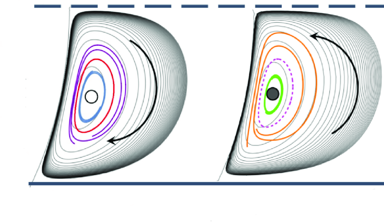
Figure 4. Particle trajectories near a stable limit cycle. (a) Particles (
 $a_p=0.2$
) spiral out (blue) or spiral into (green) a stable limit cycle (red) in a clockwise eddy. The open circle indicates the unstable fixed point, squares indicate the starting points of the particles and stars indicate the end points. (b) Close-up indicating radial distance of the particle
$a_p=0.2$
) spiral out (blue) or spiral into (green) a stable limit cycle (red) in a clockwise eddy. The open circle indicates the unstable fixed point, squares indicate the starting points of the particles and stars indicate the end points. (b) Close-up indicating radial distance of the particle
 $r_{p}(t)$
from the fixed point of the Faxen field. (c) Analytical results for the average of
$r_{p}(t)$
from the fixed point of the Faxen field. (c) Analytical results for the average of
 $r_{p}(t)$
match the solution of the dynamical system (2.10);
$r_{p}(t)$
match the solution of the dynamical system (2.10);
 $\tau$
is defined in (3.10).
$\tau$
is defined in (3.10).
3.2. Particle motion near a Faxen field fixed point
3.2.1. Linear stability analysis
The observed (slow) spiralling away from the fixed point must result from the wall corrections added to the Faxen field, whose trajectories are closed. Linearizing around the fixed point of the Faxen field yields quantitative predictions of the spiralling rate. Note that for a particle of any reasonable size
 $a_p\ll 1$
near the fixed-point position (at
$a_p\ll 1$
near the fixed-point position (at
 $y\approx -0.5$
), the gap measure will be
$y\approx -0.5$
), the gap measure will be
 $\varDelta \gg 1$
, so that wall effects are accurately described using the large-
$\varDelta \gg 1$
, so that wall effects are accurately described using the large-
 $\varDelta$
asymptotics of (B1). The leading-order wall correction terms are then considerably simpler:
$\varDelta$
asymptotics of (B1). The leading-order wall correction terms are then considerably simpler:
 \begin{equation} W_{x,large}(x,y)= -\frac {c a_{p}^3}{(y+1)^3} u_{p,F}(x,y), \end{equation}
 \begin{equation} W_{y,large}(x,y)= -\frac {15}{16}\frac {a_{p}^3}{(y+1)^2}\frac {\partial v_{p,F}(x,y)}{\partial y}, \end{equation}
where the constant
 $c$
can vary depending on the specific flow, but is
$c$
can vary depending on the specific flow, but is
 $\mathcal{O}(1)$
(Goldman et al. Reference Goldman, Cox and Brenner1967a
; Ghalia et al. Reference Ghalia, Feuillebois and Sellier2016); cf. § 2.3. Near the fixed point of the Faxen field, the
$\mathcal{O}(1)$
(Goldman et al. Reference Goldman, Cox and Brenner1967a
; Ghalia et al. Reference Ghalia, Feuillebois and Sellier2016); cf. § 2.3. Near the fixed point of the Faxen field, the
 ${\mathcal {B}_{large}}/{\mathcal {A}_{large}}$
term in
${\mathcal {B}_{large}}/{\mathcal {A}_{large}}$
term in
 $W_y$
dominates the others (
$W_y$
dominates the others (
 ${\mathcal {B}_{large}}/{\mathcal {A}_{large}} = \mathcal {O}(a_p^3),\ {\mathcal {C}_{large}}/{\mathcal {A}_{large}} = \mathcal {O}(a_p^5),\ {\mathcal {D}_{large}}/{\mathcal {A}_{large}} = \mathcal {O}(a_p^4)$
) and is the only one contributing to
${\mathcal {B}_{large}}/{\mathcal {A}_{large}} = \mathcal {O}(a_p^3),\ {\mathcal {C}_{large}}/{\mathcal {A}_{large}} = \mathcal {O}(a_p^5),\ {\mathcal {D}_{large}}/{\mathcal {A}_{large}} = \mathcal {O}(a_p^4)$
) and is the only one contributing to
 $\mathcal {O}(a_p^3)$
in (3.2). This term is still of higher
$\mathcal {O}(a_p^3)$
in (3.2). This term is still of higher
 $a_p$
order than the Faxen correction so that, in the limit of large
$a_p$
order than the Faxen correction so that, in the limit of large
 $\varDelta$
and small
$\varDelta$
and small
 $a_p$
, the wall correction is perturbatively small.
$a_p$
, the wall correction is perturbatively small.
We thus linearize (2.5) around the Faxen field fixed point (
 $x_F$
,
$x_F$
,
 $y_F$
) (given by
$y_F$
) (given by
 $\boldsymbol {u}_{p,F}=0$
) and obtain
$\boldsymbol {u}_{p,F}=0$
) and obtain
 \begin{gather} \begin{bmatrix} \dot x_{p} \\ \dot y_{p} \end{bmatrix} =\nabla {{\boldsymbol {u}_{p}\big |_{(x_F,y_F)}}} \begin{bmatrix} x-x_{F} \\ y-y_{F} \end{bmatrix} .\end{gather}
The matrix
 $\nabla {\boldsymbol {u}_{p}}\equiv A_1$
of this dynamical system can be decomposed as
$\nabla {\boldsymbol {u}_{p}}\equiv A_1$
of this dynamical system can be decomposed as
 \begin{equation} \boldsymbol {A_1}=\boldsymbol {A_F}+\boldsymbol {S}, \end{equation}
where
 $\boldsymbol {A_F}$
is the Jacobian of the Faxen field:
$\boldsymbol {A_F}$
is the Jacobian of the Faxen field:
 \begin{align} \boldsymbol {A_F}=\begin{bmatrix} \frac {\partial u_{p,F}(x,y)}{\partial x}&\frac {\partial u_{p,F}(x,y)}{\partial y} \\ \frac {\partial v_{p,F}(x,y)}{\partial x} &\frac {\partial v_{p,F}(x,y)}{\partial y} \end{bmatrix}\Bigg |_{(x_F,y_F)} \end{align}
and
 $\boldsymbol {S}$
is due to the wall corrections:
$\boldsymbol {S}$
is due to the wall corrections:
 \begin{align} \boldsymbol {S}=\begin{bmatrix} \frac {\partial W_x(x,y))}{\partial x}&\frac {\partial W_x(x,y))}{\partial y} \\[4pt] \frac {\partial W_y(x,y))}{\partial x}&\frac {\partial W_y(x,y))}{\partial y} \end{bmatrix}\Bigg |_{(x_F,y_F)} .\end{align}
The eigenvalues of
 $A_1$
are
$A_1$
are
 \begin{equation} \lambda _{1,2}^{A_1}=1/\tau \pm {\rm i}\omega _1, \end{equation}
where the real part
 $1/\tau$
is due to the wall correction
$1/\tau$
is due to the wall correction
 $S$
only, as the fixed point of the incompressible Faxen field is a centre.
$S$
only, as the fixed point of the incompressible Faxen field is a centre.
The imaginary part
 $\omega _1$
is the angular frequency of the spiralling motion, which differs only perturbatively from that of the Faxen field,
$\omega _1$
is the angular frequency of the spiralling motion, which differs only perturbatively from that of the Faxen field,
 $\omega _{1}=\omega _{F}+\mathcal {O}(a_p^{3})$
, where
$\omega _{1}=\omega _{F}+\mathcal {O}(a_p^{3})$
, where
 $\omega _{F}\equiv \sqrt {{\rm det}(A_F)}$
. To leading order, the frequency can be evaluated directly from the background flow, i.e.
$\omega _{F}\equiv \sqrt {{\rm det}(A_F)}$
. To leading order, the frequency can be evaluated directly from the background flow, i.e.
 \begin{equation} \omega _{F}=\omega _{0}+\mathcal {O}(a_p^{2})\equiv \sqrt {\frac {\partial u_(x,y)}{\partial x}\frac {\partial v(x,y)}{\partial y}-\frac {\partial u(x,y)}{\partial y}\frac {\partial v_(x,y)}{\partial x}}+\mathcal {O}(a_p^{2})\,. \end{equation}
3.2.2. Analytical prediction of particle spiralling rate
The real part of the eigenvalue (3.7) translates into an exponential growth rate of the radial distance
 $r_p$
of the particle from
$r_p$
of the particle from
 $(x_F,y_F)$
, i.e.
$(x_F,y_F)$
, i.e.
 $1/\tau = Tr(A_1)/2= Tr(S)/2$
:
$1/\tau = Tr(A_1)/2= Tr(S)/2$
:
 \begin{equation} \frac {1}{\tau }=\frac {1}{2}\left (\frac {\partial W_{x,large}(x,y)}{\partial x}+\frac {\partial W_{y,large}(x,y)}{\partial y}\right )\Big |_{(x_F,y_F)} .\end{equation}
Using the simplified wall corrections (3.1) and (3.2), neglecting higher orders of
 $a_p$
and using incompressibility, we obtain an explicit expression for the characteristic radial growth rate in terms of the background flow field only:
$a_p$
and using incompressibility, we obtain an explicit expression for the characteristic radial growth rate in terms of the background flow field only:
 \begin{equation} \frac {1}{\tau }=\frac {1}{r_{p}}\frac {{\rm d}r_{p}}{{\rm d}t}=\frac {a_{p}^3}{32(y+1)^3}\left ((16c+30)\frac {\partial v(x,y)}{\partial y}-15(y+1)\frac {\partial ^2 v(x,y)} {\partial y^2}\right )\Big |_{(x_F,y_F)}.\end{equation}
The resulting particle motion
 $r_{p} (t) =r_{p_{0}}\textit{e}^{t/\tau}$
from (3.10) with
$r_{p} (t) =r_{p_{0}}\textit{e}^{t/\tau}$
from (3.10) with
 $c=5/16$
is shown in figure 3(c), demonstrating excellent agreement with the average numerically determined distance from the fixed point of the Faxen field
$c=5/16$
is shown in figure 3(c), demonstrating excellent agreement with the average numerically determined distance from the fixed point of the Faxen field
 $(x_F,y_F)$
(oscillations are due to the non-circular shape of the orbit).
$(x_F,y_F)$
(oscillations are due to the non-circular shape of the orbit).
Although this spiralling rate will change quantitatively with
 $c$
, any
$c$
, any
 $\mathcal{O}(1)$
values of
$\mathcal{O}(1)$
values of
 $c$
will give very similar values of
$c$
will give very similar values of
 $1/\tau$
(choosing
$1/\tau$
(choosing
 $c$
a factor of 2 larger or smaller only changes the spiralling rate by
$c$
a factor of 2 larger or smaller only changes the spiralling rate by
 $\pm 12\,\%$
). In the following, we use the linear-shear value
$\pm 12\,\%$
). In the following, we use the linear-shear value
 $c=5/16$
, as it is the physical choice for particles at smaller
$c=5/16$
, as it is the physical choice for particles at smaller
 $\varDelta$
, which we discuss below.
$\varDelta$
, which we discuss below.
Near the fixed points of different vortices, the expression (3.10) is unchanged except for overall factors of powers of
 $-\zeta$
(neighbouring vortices having opposite orientation). Likewise, (3.8) remains valid up to powers of
$-\zeta$
(neighbouring vortices having opposite orientation). Likewise, (3.8) remains valid up to powers of
 $\zeta$
. Thus, a convenient dimensionless measure for the spiralling trajectories is
$\zeta$
. Thus, a convenient dimensionless measure for the spiralling trajectories is
 $\beta \equiv |\omega _0\tau |$
, valid for all vortices:
$\beta \equiv |\omega _0\tau |$
, valid for all vortices:
 \begin{equation} \beta =|\omega _0\tau |\approx \frac {0.337}{a_{p}^3}. \end{equation}
For
 $a_p\ll 1$
, the value
$a_p\ll 1$
, the value
 $\beta \gg 1$
represents the number of orbits around a Faxen field fixed point that a particle travels until its radial distance changes significantly. If
$\beta \gg 1$
represents the number of orbits around a Faxen field fixed point that a particle travels until its radial distance changes significantly. If
 $a_p$
is 0.1, for instance, such characteristic particle displacement accumulates over about 300 cycles in the vortex.
$a_p$
is 0.1, for instance, such characteristic particle displacement accumulates over about 300 cycles in the vortex.
3.3. Particle motion and manipulation in a clockwise vortex
As empirically shown by the red line in figure 3(a), the spiralling out of particles from the unstable fixed point eventually settles onto an asymptotically closed trajectory (a stable limit cycle), also reached from initial conditions closer to the wall, resulting in an inward spiral. As a motivation for the existence of this limit cycle, we compute the real part of the eigenvalues of the linearized dynamical system in the entire vortex region, i.e. (3.10) for arbitrary
 $(x,y)$
. Figure 5(a) shows that a particle spiralling out from
$(x,y)$
. Figure 5(a) shows that a particle spiralling out from
 $(x_F,y_F)$
at first encounters only positive rates of radial growth, but then a greater and greater part of the trajectory is taken up by points with negative growth rate. Eventually, on the limit cycle, the integral effect of positive and negative growth balances.
$(x_F,y_F)$
at first encounters only positive rates of radial growth, but then a greater and greater part of the trajectory is taken up by points with negative growth rate. Eventually, on the limit cycle, the integral effect of positive and negative growth balances.

Figure 5. (a) Plot of the zero contour of
 $1/\tau$
together with the stable limit cycle of an
$1/\tau$
together with the stable limit cycle of an
 $a_p=\,\rm 0.1$
particle. The open circle indicates the unstable fixed point. (b) Particle size dependence of stable limit cycle location. (c) Close-up of limit cycles for
$a_p=\,\rm 0.1$
particle. The open circle indicates the unstable fixed point. (b) Particle size dependence of stable limit cycle location. (c) Close-up of limit cycles for
 $a_p=0.01, 0.008$
showing the bandwidths of uncertainty
$a_p=0.01, 0.008$
showing the bandwidths of uncertainty
 $\delta _{1}\approx 8\times 10^{-5}$
,
$\delta _{1}\approx 8\times 10^{-5}$
,
 $\delta _{2}\approx 8\times 10^{-4}$
. (d) The minimum gap between the particle and the wall obeys a power law in particle size:
$\delta _{2}\approx 8\times 10^{-4}$
. (d) The minimum gap between the particle and the wall obeys a power law in particle size:
 $\Delta _{min}+1\propto a_{p}^{\alpha }$
, where
$\Delta _{min}+1\propto a_{p}^{\alpha }$
, where
 $\alpha \approx -0.92$
.
$\alpha \approx -0.92$
.
How does the limit cycle location depend on particle size? As the spiralling rate decreases dramatically with smaller
 $a_p$
according to (3.11), direct forward integration of (2.5) to the limit cycle is very time-consuming. Instead, we adopt a bisection scheme, integrating from an initial
$a_p$
according to (3.11), direct forward integration of (2.5) to the limit cycle is very time-consuming. Instead, we adopt a bisection scheme, integrating from an initial
 $x$
position until the same
$x$
position until the same
 $x$
coordinate is reached again, registering the change
$x$
coordinate is reached again, registering the change
 $\Delta y$
in the
$\Delta y$
in the
 $y$
coordinate. Iterating between initial conditions of positive and negative
$y$
coordinate. Iterating between initial conditions of positive and negative
 $\Delta y$
, we find the position of periodic trajectories with great accuracy.
$\Delta y$
, we find the position of periodic trajectories with great accuracy.
We plot the stable limit cycle locations for different particle sizes in figure 5(b). Note that for reasonably small
 $a_p$
even the point of closest approach to the wall has
$a_p$
even the point of closest approach to the wall has
 $\varDelta =\Delta _{min}\gg 1$
, so that using the large-
$\varDelta =\Delta _{min}\gg 1$
, so that using the large-
 $\varDelta$
approximations of
$\varDelta$
approximations of
 $\mathcal {A},\ \mathcal {B},\ \mathcal {C}\text{ and }\mathcal {D}$
from Appendix B is quantitatively accurate. As the particle gets smaller, the limit cycle grows, with a minimum distance
$\mathcal {A},\ \mathcal {B},\ \mathcal {C}\text{ and }\mathcal {D}$
from Appendix B is quantitatively accurate. As the particle gets smaller, the limit cycle grows, with a minimum distance
 $h_{min}$
closer to the wall, though
$h_{min}$
closer to the wall, though
 $h_{min}$
decreases very slowly for very small
$h_{min}$
decreases very slowly for very small
 $a_p$
. Due to the exponential
$a_p$
. Due to the exponential
 $x$
-dependence of the flow field components resulting from (2.2), we need to control for numerical errors in forward integration. Carefully evaluating (for a given
$x$
-dependence of the flow field components resulting from (2.2), we need to control for numerical errors in forward integration. Carefully evaluating (for a given
 $a_p$
) the limit cycles starting from different initial positions, we obtain a band of uncertainty around the mean limit cycle. Figure 5(c) shows that this uncertainty
$a_p$
) the limit cycles starting from different initial positions, we obtain a band of uncertainty around the mean limit cycle. Figure 5(c) shows that this uncertainty
 $\delta$
increases as
$\delta$
increases as
 $a_p$
decreases. With the standard numerical accuracy and scheme we used, uncertainty bands begin to overlap for
$a_p$
decreases. With the standard numerical accuracy and scheme we used, uncertainty bands begin to overlap for
 $a_p\lesssim 0.005$
. Accurate data for smaller
$a_p\lesssim 0.005$
. Accurate data for smaller
 $a_p$
could be accessed with more powerful algorithms or CPUs, but this is not our focus here. Restricting ourselves to
$a_p$
could be accessed with more powerful algorithms or CPUs, but this is not our focus here. Restricting ourselves to
 $a_p\geqslant 0.008$
, we show
$a_p\geqslant 0.008$
, we show
 $h_{min}/a_p=\Delta _{min}+1$
as a function of
$h_{min}/a_p=\Delta _{min}+1$
as a function of
 $a_p$
in figure 5(d), demonstrating an accurate power law (all uncertainties are below the symbol size) of the form
$a_p$
in figure 5(d), demonstrating an accurate power law (all uncertainties are below the symbol size) of the form
 \begin{equation} (\Delta _{min} + 1) \propto a_p^\alpha , \end{equation}
with an exponent
 $\alpha \approx -0.92$
. Note that
$\alpha \approx -0.92$
. Note that
 $\Delta _{min}$
diverges as
$\Delta _{min}$
diverges as
 $a_p\to 0$
so that the
$a_p\to 0$
so that the
 $\varDelta \gg 1$
limit becomes ever more accurate. Indeed, none of the quantitative results of figure 5(d) change when the full or asymptotic expressions for the wall effects are used. The scaling implies
$\varDelta \gg 1$
limit becomes ever more accurate. Indeed, none of the quantitative results of figure 5(d) change when the full or asymptotic expressions for the wall effects are used. The scaling implies
 $h_{min}\propto a_p^\eta$
with
$h_{min}\propto a_p^\eta$
with
 $\eta \approx 0.08$
, confirming the very slow approach of the limit cycles towards the wall.
$\eta \approx 0.08$
, confirming the very slow approach of the limit cycles towards the wall.
For particle sizes relevant to microfluidics, this effect means that there is a practical boundary for how close to the wall the particles can approach. Taking the characteristic (half-width) length of the channel to be 50
 $\,{\unicode{x03BC}}$
m, a
$\,{\unicode{x03BC}}$
m, a
 $1\,{\unicode{x03BC}}$
m particle (
$1\,{\unicode{x03BC}}$
m particle (
 $a_p=0.02$
) will not approach the wall any closer than 7.8
$a_p=0.02$
) will not approach the wall any closer than 7.8
 $\,{\unicode{x03BC}}\rm m$
. Moreover, using the locations of stable limit cycles to separate particles becomes very difficult for small particles. For practical situations, the difference between the
$\,{\unicode{x03BC}}\rm m$
. Moreover, using the locations of stable limit cycles to separate particles becomes very difficult for small particles. For practical situations, the difference between the
 $h_{min}$
for a 1
$h_{min}$
for a 1
 $\,{\unicode{x03BC}}\rm m$
particle and a 2.5
$\,{\unicode{x03BC}}\rm m$
particle and a 2.5
 $\,{\unicode{x03BC}} m$
particle is only 0.7
$\,{\unicode{x03BC}} m$
particle is only 0.7
 $\,{\unicode{x03BC}} m$
. Separation by size can be further compromised by the presence of Brownian motion. Using characteristic time scales
$\,{\unicode{x03BC}} m$
. Separation by size can be further compromised by the presence of Brownian motion. Using characteristic time scales
 $\tau$
from (3.11) to estimate positional uncertainty due to Brownian diffusion, we find that an
$\tau$
from (3.11) to estimate positional uncertainty due to Brownian diffusion, we find that an
 $a_p=5\,{\unicode{x03BC}}\rm m$
particle is hardly affected, while the position of a strongly colloidal
$a_p=5\,{\unicode{x03BC}}\rm m$
particle is hardly affected, while the position of a strongly colloidal
 $a_p=1\,{\unicode{x03BC}}\rm m$
particle will be spread out over several
$a_p=1\,{\unicode{x03BC}}\rm m$
particle will be spread out over several
 ${\unicode{x03BC}}\rm m$
.
${\unicode{x03BC}}\rm m$
.
Despite these caveats, the ability to concentrate particles on a limit cycle trajectory without inertial effects purely because of the background flow geometry is of fundamental interest. It is encouraging that the location of this limit cycle for small particles can be determined entirely within the large-
 $\varDelta$
approximation, i.e. without the intricate details of near-wall corrections or lubrication limits. This gives confidence in not only the qualitative but also the quantitative description of the phenomenon: when placed in certain bounded vortical Stokes flows, small spherical particles, even when neutrally buoyant, will eventually accumulate on well-defined closed trajectories.
$\varDelta$
approximation, i.e. without the intricate details of near-wall corrections or lubrication limits. This gives confidence in not only the qualitative but also the quantitative description of the phenomenon: when placed in certain bounded vortical Stokes flows, small spherical particles, even when neutrally buoyant, will eventually accumulate on well-defined closed trajectories.

Figure 6. Particle trajectories near an unstable limit cycle. (a) Particles (
 $a_p=0.1$
) spiral out (orange) towards the wall or spiral into (purple) a fixed point from an unstable limit cycle (dashed red) in a counterclockwise eddy. A particular spiralling-out trajectory is shown in blue. The filled circle indicates the stable fixed point, squares indicate the particle starting points and stars indicate the particle end points. (b) Close-up of the close approach to the wall of the trajectory from (a). The solid portion of the trajectory shows approximately exponential thinning of the gap, shown in the semi-logarithmic plot of (c). The black dashed line indicates the exponential behaviour from the wall-expansion approximation (3.13). The red dot-dashed line corresponds to a surface-to-surface approach of 5 nm distance for a 5 μm particle in a channel of 50 μm half-width.
$a_p=0.1$
) spiral out (orange) towards the wall or spiral into (purple) a fixed point from an unstable limit cycle (dashed red) in a counterclockwise eddy. A particular spiralling-out trajectory is shown in blue. The filled circle indicates the stable fixed point, squares indicate the particle starting points and stars indicate the particle end points. (b) Close-up of the close approach to the wall of the trajectory from (a). The solid portion of the trajectory shows approximately exponential thinning of the gap, shown in the semi-logarithmic plot of (c). The black dashed line indicates the exponential behaviour from the wall-expansion approximation (3.13). The red dot-dashed line corresponds to a surface-to-surface approach of 5 nm distance for a 5 μm particle in a channel of 50 μm half-width.
3.4. Particle motion and manipulation in a counterclockwise vortex
Any vortex adjacent to a clockwise vortex like the one discussed in § 3.2 is counterclockwise and congruent in geometry. For example, the vortex indicated by the green frame in figure 3(a) has flow exactly reversed from the yellow-framed vortex (and a factor
 $\zeta$
slower). Because of the time reversibility of Stokes flow and the fact that all wall effects result from the background Stokes flow and its derivatives, the behaviour of particles on trajectories is also time-reversed. Thus, the fixed point in a counterclockwise vortex is stable,
$\zeta$
slower). Because of the time reversibility of Stokes flow and the fact that all wall effects result from the background Stokes flow and its derivatives, the behaviour of particles on trajectories is also time-reversed. Thus, the fixed point in a counterclockwise vortex is stable,
 $ 1/\tau $
changes sign and
$ 1/\tau $
changes sign and
 $\beta$
stays the same by definition. The limit cycle for a given
$\beta$
stays the same by definition. The limit cycle for a given
 $a_p$
is unstable but is congruent in shape with the stable cycle discussed before. Particles spiral inward from the unstable limit cycle towards the fixed points but spiral outward when placed outside the limit cycle (figure 6
a). The latter case is of prime interest because it allows particles to approach the wall more and more closely. As the gap between particle and wall diminishes, any short-ranged intermolecular attractive force (e.g. van der Waals force) whose reach is often in the nanometre range (Hirschfelder et al. Reference Hirschfelder1954; Batsanov Reference Batsanov2001) can take over and lead to attachment (sticking) of the particle to the wall. This general mechanism (hydrodynamics allowing a particle to get close enough to a wall to stick by short-ranged attraction) has been acknowledged before (Friedlander et al. Reference Friedlander2000; Humphries Reference Humphries2009), but the case discussed here allows for quantitative predictions.
$a_p$
is unstable but is congruent in shape with the stable cycle discussed before. Particles spiral inward from the unstable limit cycle towards the fixed points but spiral outward when placed outside the limit cycle (figure 6
a). The latter case is of prime interest because it allows particles to approach the wall more and more closely. As the gap between particle and wall diminishes, any short-ranged intermolecular attractive force (e.g. van der Waals force) whose reach is often in the nanometre range (Hirschfelder et al. Reference Hirschfelder1954; Batsanov Reference Batsanov2001) can take over and lead to attachment (sticking) of the particle to the wall. This general mechanism (hydrodynamics allowing a particle to get close enough to a wall to stick by short-ranged attraction) has been acknowledged before (Friedlander et al. Reference Friedlander2000; Humphries Reference Humphries2009), but the case discussed here allows for quantitative predictions.
Figure 6(b) exemplifies a particle trajectory that approaches very close to the wall, with a nearly normal initial approach and a subsequent piece of trajectory nearly parallel to the wall. Here,
 $\varDelta \ll 1$
characterizes the trajectory and this is the only scenario in the present work where the variable expansion method for particle normal velocity (2.15) is necessary. The semi-logarithmic plot versus time in figure 6(c) shows that the ‘near-parallel’ portion contains a stretch of approximately exponential decay of the (relative) gap
$\varDelta \ll 1$
characterizes the trajectory and this is the only scenario in the present work where the variable expansion method for particle normal velocity (2.15) is necessary. The semi-logarithmic plot versus time in figure 6(c) shows that the ‘near-parallel’ portion contains a stretch of approximately exponential decay of the (relative) gap
 $\varDelta$
. Indeed, this behaviour follows from a series to leading order in small
$\varDelta$
. Indeed, this behaviour follows from a series to leading order in small
 $\varDelta$
of (2.15), i.e. the wall-expansion limit of
$\varDelta$
of (2.15), i.e. the wall-expansion limit of
 $y_E\to -1$
. Here, (2.14) simplifies to
$y_E\to -1$
. Here, (2.14) simplifies to
 \begin{equation} \frac {{\rm d} \Delta }{{\rm d}t}=1.6147a_p\kappa (x)\varDelta , \end{equation}
where
 $\kappa (x) = {\partial ^2v}/{\partial y^2}(x,-1)$
is the background flow curvature at the wall, and the prefactor was first derived in Goren & O’Neill (Reference Goren and O’Neill1971) and confirmed in Rallabandi et al. (Reference Rallabandi, Hilgenfeldt and Stone2017). The trajectory part showing the exponential approach (the solid portion in figure 6
b,c) indicates slow motion in the
$\kappa (x) = {\partial ^2v}/{\partial y^2}(x,-1)$
is the background flow curvature at the wall, and the prefactor was first derived in Goren & O’Neill (Reference Goren and O’Neill1971) and confirmed in Rallabandi et al. (Reference Rallabandi, Hilgenfeldt and Stone2017). The trajectory part showing the exponential approach (the solid portion in figure 6
b,c) indicates slow motion in the
 $x$
direction, so that
$x$
direction, so that
 $\kappa (x)$
is nearly constant. We fix the
$\kappa (x)$
is nearly constant. We fix the
 $x$
value as that of the turning point (point of maximum curvature) of the trajectory, here
$x$
value as that of the turning point (point of maximum curvature) of the trajectory, here
 $x\approx 0.991$
. Using this value in (3.13) gives an exponential behaviour (dashed line in figure 6
c) in good agreement with the approach of the trajectory to the wall. This behaviour remains robust to changes of the exact modelling of the expansion point locations
$x\approx 0.991$
. Using this value in (3.13) gives an exponential behaviour (dashed line in figure 6
c) in good agreement with the approach of the trajectory to the wall. This behaviour remains robust to changes of the exact modelling of the expansion point locations
 $y_E$
in (2.13).
$y_E$
in (2.13).
This exponential approach to a wall accords with the general derivations of Brady et al., showing that the gap between solid surfaces in Stokes flow can never vanish in finite time (Brady & Bossis Reference Brady and Bossis1988; Claeys & Brady Reference Claeys and Brady1989, Reference Claeys and Brady1993). In a practical situation, the rapidly decaying gap width leads to sticking by short-range interaction at a well-defined position after a well-defined time. If figure 6(c) pertains to a microfluidic situation exemplified by a channel half-width of 50 μm and a particle radius of 5 μm, the red dashed line indicates a gap of 5 nm between particle and wall, at the low end of the typical range of van der Waals forces (Israelachvili Reference Israelachvili1974). The particle can, therefore, be expected to stick at a time and location entirely determined by the geometry of the background flow. Thus, we demonstrate here how, in a pure Stokes flow, particles can be driven towards boundaries and forced to stick to a wall in predictable locations. Note that conceptually, a counterclockwise vortex allows for the concentration of randomly distributed particles in two locations: the stable fixed point near the centre of the vortex and the well-defined small region of wall sticking. Both alternatives provide practically relevant protocols for filtering in microfluidic devices. Particles placed inside the unstable limit cycle will be concentrated at the fixed point, while particles placed outside the unstable limit cycle will be deposited onto a surface.
Our single-particle formalism implicitly assumes the limit of dilute particle concentration in a microfluidics application. Including effects of particle–particle interaction is a desirable future extension of this approach in order to assess non-inertial effects in particle-laden flows important to practical applications (Guha Reference Guha2008).
4. Conclusions
We have quantitatively shown that force-free particles placed in an internal Stokes flow can be systematically displaced in a variety of ways through purely hydrodynamic interactions with the enclosing walls. Since a particle cannot contact a wall in finite time, a typical trajectory has a portion of approaching the wall and a portion of receding, governed by the background flow and the wall corrections derived from it. If the approaching and receding parts of the flow are symmetric, displacement effects off a streamline will cancel out. Thus, a Stokes flow that induces net particle displacement must break wall-parallel symmetry.
For practical use, vortical flows are advantageous, where the effects of many approaching/receding events can accumulate. However, if the vortex is symmetrically confined between walls, the net displacement effects induced by both walls will again cancel, and the particle trajectory must close. For net cumulative displacement, the vortex must, therefore, break wall-normal symmetry as well, for example by being confined between no-slip and no-stress boundaries. A net-transport internal Stokes flow thus breaks symmetries in both directions by particle–wall interactions, which act as perturbations on the Faxen flow trajectories. This is in agreement with recent experimental results that record permanent displacements of fibres passing by obstacles of symmetry-broken shape (Li et al. Reference Li, Bielinski, Lindner, du Roure and Delmotte2024). For such non-spherical particles (whether rigid or elastic), the effect of a single particle–boundary encounter could be much enhanced, as the wall effects affect different parts of the particle differently, and the overall torque balance will influence the resulting displacement. The study of this case will be the subject of future work.
Our formalism predicts how the particles approach or recede from fixed points at the centre of the vortices, and how the particles accumulate at stable limit cycles, whose locations are dependent on particle size. When placed in certain bounded vortical Stokes flows, small spherical particles, even when neutrally buoyant, will eventually accumulate on well-defined closed trajectories. In practical applications, the accumulated particles can be induced to aggregate or react with each other. We can also predict how particles move away from unstable limit cycles towards boundaries. Generically, such trajectories must eventually lead to exponential thinning of the fluid layer between particle and wall. Thus, submicrometre distances are reached, leading to sticking in predictable locations by short-range forces. Such adhesion to walls in Stokes flows adds a simple and controllable tool to studies of sticking phenomena, which have been investigated for some time. Researchers have investigated particles captured, filtered and deposited on surfaces in low-Reynolds flow by short-range interactions with the wall when approaching (Arias-Zugasti et al. Reference Arias-Zugasti, Rosner and Fernandez de la Mora2019; Espinosa-Gayosso et al. Reference Espinosa-Gayosso, Ghisalberti, Ivey and Jones2012). Applications include fibre filtration (Tien et al. Reference Tien, Wang and Barot1977; Myojo et al. Reference Myojo, Kanaoka and Emi1984) and fog meshes (Park et al. Reference Park, Chhatre, Srinivasan, Cohen and McKinley2013) inspired by moisture-collecting desert beetles (Parker & Lawrence Reference Parker and Lawrence2001; King et al. Reference King, Shahrokhian, Chan, Feng and Gazzola2022). This is also related to the functionality of facemasks in the recent COVID-19 pandemic (Howard et al. Reference Howard2021). However, most of the work emphasizes the dependence of particle deposition probabilities on the finite Stokes number in the flow, while few studies focus on the Stokes flow regime or acknowledge that any filtration effect is possible in this limit.
Let us estimate the rate of particle drift across streamlines in dimensional terms. Taking the length scale (channel half-width) as
 $H=50$
μm, we want to ensure that the channel Reynolds number
$H=50$
μm, we want to ensure that the channel Reynolds number
 $Re=HU/\nu$
for aqueous solutions (
$Re=HU/\nu$
for aqueous solutions (
 $\nu \sim 10^{-6}\,\rm m^{^2}\rm s^-{^1}$
) is less than
$\nu \sim 10^{-6}\,\rm m^{^2}\rm s^-{^1}$
) is less than
 $10^{-2}$
along the particle trajectories, even in regions of the highest speed
$10^{-2}$
along the particle trajectories, even in regions of the highest speed
 $U$
. Given this constraint and assuming
$U$
. Given this constraint and assuming
 $a_p=5$
μm, the time scale
$a_p=5$
μm, the time scale
 $\tau$
from (3.10) is
$\tau$
from (3.10) is
 $\approx 57\,\rm s$
so that a significant radial displacement is expected on a time scale of minutes. For larger particles, this time scale decreases rapidly (
$\approx 57\,\rm s$
so that a significant radial displacement is expected on a time scale of minutes. For larger particles, this time scale decreases rapidly (
 $\propto a_p^{-3}$
), and the process can also be sped up by using a solution of higher viscosity.
$\propto a_p^{-3}$
), and the process can also be sped up by using a solution of higher viscosity.
The Moffatt eddy flow discussed here is convenient because of its closed analytical form. However, it would be extremely difficult to set up experimentally due to the exponential decay of the flow speed with
 $x$
and the need to drive the flow far away from the field of view. The exponential dependence of speed on coordinates also makes the Reynolds number constraint for Stokes flow extremely stringent. Nevertheless, the principles of displacement and the scaling of the wall effects are not specific to this flow and will be robust in any symmetry-breaking vortical Stokes flow, and the modelling equations for the crucial wall-normal displacement such as (2.11) and (2.15) are valid for arbitrary background flow.
$x$
and the need to drive the flow far away from the field of view. The exponential dependence of speed on coordinates also makes the Reynolds number constraint for Stokes flow extremely stringent. Nevertheless, the principles of displacement and the scaling of the wall effects are not specific to this flow and will be robust in any symmetry-breaking vortical Stokes flow, and the modelling equations for the crucial wall-normal displacement such as (2.11) and (2.15) are valid for arbitrary background flow.
Cavity flows are a class of vortical flows that are practically used in microfluidic devices at low and vanishing Reynolds numbers. In the Stokes limit, they can be expressed as infinite sums of Moffatt solutions (Shankar Reference Shankar1993; Shankar & Deshpande Reference Shankar and Deshpande2000) and can be driven by rotating cylinders (Hellou & Coutanceau Reference Hellou and Coutanceau1992; Hellou Reference Hellou2001) or by superimposed transport flows (Hellou & Bach Reference Hellou and Bach2011). Because of the linearity of the Stokes equations and the velocity corrections, such flows do not pose principal difficulties to the present formalism. These finite-domain modifications of Moffatt’s solutions have a less severe ratio of driving velocity to the eddy velocity scale (the analogue of
 $\textit{e}^{p\pi /q}$
), and it is thus much easier to fulfil the conditions of small
$\textit{e}^{p\pi /q}$
), and it is thus much easier to fulfil the conditions of small
 $Re$
.
$Re$
.
It is instructive to compare the scaling of the migration velocity of small particles far from the wall (
 $\varDelta \gg 1$
) with that of approaches using particle inertia. In a number of approaches quantifying the effect of steady inertia (Ho & Leal Reference Ho and Leal1974; Schonberg & Hinch Reference Schonberg and Hinch1989; Asmolov & McLaughlin Reference Asmolov and McLaughlin1999; Di Carlo et al. Reference Di Carlo, Dino, Daniel, Ronald and Toner2007; Hood et al. Reference Hood, Lee and Roper2015) the migration speed for force-free particles is proportional to
$\varDelta \gg 1$
) with that of approaches using particle inertia. In a number of approaches quantifying the effect of steady inertia (Ho & Leal Reference Ho and Leal1974; Schonberg & Hinch Reference Schonberg and Hinch1989; Asmolov & McLaughlin Reference Asmolov and McLaughlin1999; Di Carlo et al. Reference Di Carlo, Dino, Daniel, Ronald and Toner2007; Hood et al. Reference Hood, Lee and Roper2015) the migration speed for force-free particles is proportional to
 $a_p^3$
, the same scaling as our result (3.2). In approaches using oscillatory inertia (Agarwal et al. Reference Agarwal, Chan, Rallabandi, Gazzola and Hilgenfeldt2021,Reference Agarwal, Upadhyay, Bhosale, Gazzola and Hilgenfeldt2024), the scaling varies from
$a_p^3$
, the same scaling as our result (3.2). In approaches using oscillatory inertia (Agarwal et al. Reference Agarwal, Chan, Rallabandi, Gazzola and Hilgenfeldt2021,Reference Agarwal, Upadhyay, Bhosale, Gazzola and Hilgenfeldt2024), the scaling varies from
 $a_p^3$
for small Stokes number to
$a_p^3$
for small Stokes number to
 $a_p^4$
for large Stokes number. Thus, the strictly non-inertial effects described in the present work show scaling equal to or even more favourable than inertial techniques for small particles. It should be noted that at low (non-zero)
$a_p^4$
for large Stokes number. Thus, the strictly non-inertial effects described in the present work show scaling equal to or even more favourable than inertial techniques for small particles. It should be noted that at low (non-zero)
 $Re$
the walls of a microfluidic device will almost always be close enough to the particle to enable modelling as in Ho & Leal (Reference Ho and Leal1974) or Hood et al. (Reference Hood, Lee and Roper2015), i.e. the effects of inertia at large distances are not present. This is why Saffman lift (Saffman Reference Saffman1965), an unbounded-flow effect, should not be directly compared with these results.
$Re$
the walls of a microfluidic device will almost always be close enough to the particle to enable modelling as in Ho & Leal (Reference Ho and Leal1974) or Hood et al. (Reference Hood, Lee and Roper2015), i.e. the effects of inertia at large distances are not present. This is why Saffman lift (Saffman Reference Saffman1965), an unbounded-flow effect, should not be directly compared with these results.
In closing, we note that oscillatory-flow microfluidic set-ups used for fast particle manipulation often result both in inertial forces on particles (Agarwal et al. Reference Agarwal, Chan, Rallabandi, Gazzola and Hilgenfeldt2021,Reference Agarwal, Upadhyay, Bhosale, Gazzola and Hilgenfeldt2024) and in the generation of steady vortical streaming flow of low Reynolds number (Rallabandi et al. Reference Rallabandi, Wang and Hilgenfeldt2014; Thameem et al. Reference Thameem, Rallabandi and Hilgenfeldt2017; Rallabandi et al. Reference Rallabandi, Hilgenfeldt and Stone2017). The effects discussed in the present work can thus be exploited and optimized together with inertial effects, leading to better protocols for the accumulation, concentration, deflection and sorting of microparticles.
Supplementary movie.
Supplementary movie is available at https://doi.org/10.1017/jfm.2025.64.
Acknowledgements.
The authors acknowledge valuable and inspiring conversations with J. Brady, C. Duprat, A. Lindner, B. Rallabandi and H. Stone.
Declaration of interests.
The authors report no conflict of interest.
Appendix A
To get the shear coefficient of the particle parallel velocity
 $f(\varDelta )$
, we start with the form from Pasol et al. (Reference Pasol, Martin, Ekiel-Jeżewska, Wajnryb, Bławzdziewicz and Feuillebois2011):
$f(\varDelta )$
, we start with the form from Pasol et al. (Reference Pasol, Martin, Ekiel-Jeżewska, Wajnryb, Bławzdziewicz and Feuillebois2011):
 \begin{equation} \begin{aligned} f(\varDelta )&=1-\left [1-a\log \left(1-\frac {1}{1+\varDelta }\right)-b_1\left(\frac {1}{1+\varDelta }\right)-b_2\left(\frac {1}{1+\varDelta }\right)^2 \right . \\& \left . -b_3\left(\frac {1}{1+\varDelta }\right)^3-b_4\left(\frac {1}{1+\varDelta }\right)^4\right ]^{-1} .\end{aligned} \end{equation}
We take a series expansion of
 $f(\varDelta )$
as
$f(\varDelta )$
as
 $\varDelta \to \infty$
to the order
$\varDelta \to \infty$
to the order
 $\Delta ^3$
:
$\Delta ^3$
:
 \begin{equation} \begin{aligned} &f(\varDelta )=-\frac {-a+b_1}{\varDelta }-\frac {a^2+a(\frac {1}{2}-2b_1)-b_1+b_1^{2}+b_2}{\Delta ^2}\\&\!\!-\frac {-a^3+b_1-2b_1^2+b_1^3+a^2(-1+3b_1)-2b_2+2b_1b_2-\frac {1}{3}a(1-9b_1+9b_1^2+6b_2)\!+b_3}{\Delta ^3}\\&+H.O.T. \end{aligned} \end{equation}
According to Goldman et al. (Reference Goldman, Cox and Brenner1967
a) as
 $\varDelta \to \infty$
,
$\varDelta \to \infty$
,
 $f(\varDelta )\simeq 1-\frac {5}{16}\Delta ^{-3}$
, which means that the order
$f(\varDelta )\simeq 1-\frac {5}{16}\Delta ^{-3}$
, which means that the order
 $\Delta ^{-1}$
and
$\Delta ^{-1}$
and
 $\Delta ^{-2}$
must vanish, resulting in
$\Delta ^{-2}$
must vanish, resulting in
 \begin{equation} a-b_1=0\, \qquad a^2+a\left(\frac {1}{2}-2b_1 \right)-b_1+b_1^{2}+b_2=0, \end{equation}
so that
 $b_1=a$
and
$b_1=a$
and
 $b_2= a/2$
. With
$b_2= a/2$
. With
 $b_1$
and
$b_1$
and
 $b_2$
substituted, matching with Goldman’s large-
$b_2$
substituted, matching with Goldman’s large-
 $\varDelta$
asymptotic expression obtains
$\varDelta$
asymptotic expression obtains
 \begin{equation} b_3=\frac {5}{16}+\frac {a}{3}\,. \end{equation}
We then take a series expansion of
 $f(\varDelta )$
as
$f(\varDelta )$
as
 $\varDelta \to 0$
to leading order:
$\varDelta \to 0$
to leading order:
 \begin{equation} f(\varDelta )\approx 1+\frac {2}{3a+2(-1+b_3+b_4)+2a\log (\varDelta )} .\end{equation}
According to Williams (Reference Williams1994) as
 $\varDelta \to 0$
,
$\varDelta \to 0$
,
 $f(\varDelta )\simeq 1-\frac {1}{0.66-0.269\log (\frac {\varDelta }{1+\varDelta })}$
. By matching all the parameters, we obtain
$f(\varDelta )\simeq 1-\frac {1}{0.66-0.269\log (\frac {\varDelta }{1+\varDelta })}$
. By matching all the parameters, we obtain
 $a=0.269$
and
$a=0.269$
and
 \begin{equation} \frac {1}{2}\left (-3a-2(-1+b_3+b_4) \right )=0.66. \end{equation}
Combined with equations (A4) and (A6), this determines
 $b_3=-0.223$
and
$b_3=-0.223$
and
 $b_4=0.159$
. All parameters of (A1) are now specified, and the result is equation (2.8).
$b_4=0.159$
. All parameters of (A1) are now specified, and the result is equation (2.8).
Appendix B
The scalar quantities
 $\mathcal {A}$
,
$\mathcal {A}$
,
 $\mathcal {B}$
,
$\mathcal {B}$
,
 $\mathcal {C}$
and
$\mathcal {C}$
and
 $\mathcal {D}$
are dimensionless hydrodynamic resistances depending on
$\mathcal {D}$
are dimensionless hydrodynamic resistances depending on
 $\varDelta$
. The analytical expressions for
$\varDelta$
. The analytical expressions for
 $\mathcal {A}$
,
$\mathcal {A}$
,
 $\mathcal {B}$
,
$\mathcal {B}$
,
 $\mathcal {C}$
and
$\mathcal {C}$
and
 $\mathcal {D}$
are given (as infinite sums) in Rallabandi et al. (Reference Rallabandi, Hilgenfeldt and Stone2017). For large separations (
$\mathcal {D}$
are given (as infinite sums) in Rallabandi et al. (Reference Rallabandi, Hilgenfeldt and Stone2017). For large separations (
 $\varDelta \gg 1$
), one obtains four hydrodynamic resistances at leading order:
$\varDelta \gg 1$
), one obtains four hydrodynamic resistances at leading order:
 \begin{equation} \mathcal {A}_{large} = 1+\frac {9}{8}\Delta ^{-1},\quad \mathcal {B}_{large} = \frac {15}{16}\Delta ^{-1},\quad \mathcal {C}_{large} = \frac {21}{32}\Delta ^{-3} , \quad \mathcal {D}_{large} = \frac {1}{3}+\frac {3}{8}\Delta ^{-1}. \end{equation}
The ratios used in the equations for velocity corrections are, to leading order,
 \begin{equation} \frac {\mathcal {B}_{large}}{\mathcal {A}_{large}}\approx \frac {15}{16}\Delta ^{-2},\quad \frac {\mathcal {C}_{large}}{\mathcal {A}_{large}}\approx \frac {21}{32}\Delta ^{-3}, \quad \frac {\mathcal {D}_{large}}{\mathcal {A}_{large}}\approx \frac {1}{3}\,. \end{equation}
For small separations (
 $\varDelta \ll 1$
), one obtains four hydrodynamic resistances to leading order:
$\varDelta \ll 1$
), one obtains four hydrodynamic resistances to leading order:
 \begin{equation} \begin{aligned} \mathcal {A}_{small} &= \Delta ^{-1}+\frac {1}{5}\log \Delta ^{-1}+0.9713,\quad \mathcal {B}_{small} = \Delta ^{-1}-\frac {4}{5}\log \Delta ^{-1}+0.3070,\quad \\ \mathcal {C}_{small} &= \Delta ^{-1}-\frac {14}{5}\log \Delta ^{-1}+3.7929 , \quad \mathcal {D}_{small} = \log \Delta ^{-1}-0.9208\,. \end{aligned} \end{equation}
These results can be used to obtain the numerical prefactor of the wall-expansion limit equation (3.13).


 Open access