


1. Introduction
Primary cementing is used to seal every oil and gas well (Nelson & Guillot Reference Nelson and Guillot2006), of which there are many millions globally. In this operation a sequence of fluids is pumped down the inside of a steel casing, to the bottom of a well, returning upwards in the annular space between formation wall and exterior of the casing. The objective is to remove the drilling fluid and other residue from the well, replacing it with a cement slurry, which then hydrates and seals the well to prevent subsurface leakage. This paper focuses on the fluid mechanics of primary cementing, which mainly consists of a fluid–fluid displacement flow along a narrow eccentric annular duct. This is a sequel to Renteria & Frigaard (Reference Renteria and Frigaard2020) (referred to as Part 1), in which we focused on results of scaled laboratory experiments. Here, we compare experiments with three-dimensional (3-D) computations and use these same computations to probe deeper into the flow structure.
The study considers only horizontal wells, which have been increasingly common over the past 25 years. For example, in British Columbia, vertical wells accounted for  $>$75 % of wells drilled prior to 2000, but
  $\approx$95 % of wells drilled in the last decade have been horizontal (Trudel et al. Reference Trudel, Bizhani, Zare and Frigaard2019). Unfortunately, many of these recent wells appear more susceptible to leakage, which explains our interest. Methane is a powerful greenhouse gas and leakage can lead to polluted aquifers, damaged subsurface ecosystems, methane emissions and reduced well productivity. It is difficult to locate and expensive to fix. An introduction to the primary cementing literature is given in Part 1.
The experiments in Renteria & Frigaard (Reference Renteria and Frigaard2020) were performed in a clear acrylic laboratory apparatus, using transparent (and dyed) fluids of differing densities and viscosities. The annulus was uniformly eccentric and horizontal. Comparisons were made with predictions from the theory developed by Carrasco-Teja et al. (Reference Carrasco-Teja, Frigaard, Seymour and Storey2008) and with simulations using the (laminar) model of Maleki & Frigaard (Reference Maleki and Frigaard2017), which is a 2-D gap-averaged (2DGA) model. Approximately 300 experiments were conducted. Two main behaviours were observed: top side and slumping displacements, which refer to whether the main displacement front advances along the top or bottom of the annulus. These flow types are predicted well by the 2DGA model. The 2DGA approach was also reasonably effective at predicting steady and unsteady displacements in the experiments.
However, other features of the experiments were not predicted as well. The main discrepancy comes from gap averaging of the model, which is part of the Hele-Shaw approach. This negates dispersion on the scale of the annular gap. Other secondary flows may lead to dispersion in the 2DGA model. Dispersion was significant in many of the experiments of Part 1. One indication of this fact is that, in most cases, the front velocities determined from the experiments exceeded those of the model. Dispersion has also been found in other experimental studies in near-horizontal annuli (Lund et al. Reference Lund, Ytrehus, Taghipour, Divyankar and Stavanger2018; Renteria et al. Reference Renteria, Maleki, Frigaard, Lund, Taghipour and Ytrehus2019), where arrival times of displacing fluids at conductivity probes are notably faster than 2DGA predictions and spreading of the front is more extensive.
The inability of these simpler models to reproduce the degree of dispersion is a key motivation for the 3-D computational study in this paper. Simulations also allow for independent parameter variations in a way that experiments sometimes do not. Three-dimensional simulations of annular displacement flows were first developed in the late 1990s but were too slow for practical usage (Szabo & Hassager Reference Szabo and Hassager1997; Vefring et al. Reference Vefring, Bjorkevoll, Hansen, Sterri, Saevareid, Aas and Merlo1997). In recent years, interest has revived in these methods as open source and other computational codes have become widely accessible and multi-processor computations have made such calculations manageable at reasonable resolutions over increasingly long annuli and even for non-Newtonian fluids, e.g. Kragset & Skadsem (Reference Kragset and Skadsem2018), Etrati & Frigaard (Reference Etrati and Frigaard2019) and Skadsem et al. (Reference Skadsem, Kragset, Lund, Ytrehus and Taghipour2019). Those 3-D simulations that have been published certainly expose flow features not present in Hele-Shaw models: inertial effects and flow features on the scale of the annular gap. In particular, residual layers on the scale of the annular gap are a reality (Allouche, Frigaard & Sona Reference Allouche, Frigaard and Sona2000; Zare, Roustaei & Frigaard Reference Zare, Roustaei and Frigaard2017). When these layers outlast the displacement flow, the residual fluids form a potential means for wellbore leakage (called wet micro-annuli or mud channels).
Thus, resolution of the annular-gap flows is essential. The 3-D challenge then comes from the disparity in aspect ratios: gap width, circumference and length, if the mesh scale is set by the annular-gap dimension. Furthermore, the time scale of flow also increases proportional to the length of annulus, making the computational cost severe. Our experimental annulus has length to circumference ratio of  $\approx$78 and circumference to gap ratio of
  $\approx$26. As we will see below, we are able to simulate the experimental displacement flows effectively. However, while the latter is representative, this scaled length corresponds to 10–30 m of a real well dimension. In practice, cemented sections of well are 100s or 1000s of metres in length. Therefore, although now able to simulate useful lengths of well in three dimensions, we have a long way to go.
This paper focuses on a detailed comparison of 3-D computations with our earlier experiments. In § 2 we present an overview of the methods used here. Section 3 covers the results. We first give a visual classification of the flows, comparing with the same classification of the experiments in Part 1. The simulations are then used to look in depth at top side and slumping flows (§ 3.1.1), and the phenomenon of residual fluid left behind in the narrowest part of the annulus (§ 3.1.2). In § 3.2 we explore steady and unsteady displacement flows, showing that the simulations produce near-identical classifications to our experiments. We then explore the effects of eccentricity and viscosity ratio on the transition between top side and slumping flows (§ 3.3). In § 3.4 we explore 1-D characterizations of the spreading displacement front, via dispersive and diffusive mechanisms. The paper ends with a brief discussion and conclusions.
2. Methodology
As explained in § 1, the main aim of this paper is to explore eccentric annular displacement flows of 2 Newtonian fluids using 3-D simulation. To this end, we rely strongly on the experimental results from Part 1, both to validate the code output and to guide us in terms of the dominant phenomena. The 3-D simulations then have many advantages in terms of the flow variables computed, parameter ranges are readily accessible and there is the ability to explore beyond what is measured experimentally.
Dimensional analysis of the miscible displacement flow of 2 Newtonian fluids along a uniformly eccentric horizontal annulus shows that there are 7 different non-dimensional parameters involved. The problem is substantially simplified in the case of small gap to circumference aspect ratio  $\delta$ (i.e. a narrow gap), and where advection dominates molecular diffusion (large Péclet number,
  $Pe$). This situation is represented in the model and analysis of Carrasco-Teja et al. (Reference Carrasco-Teja, Frigaard, Seymour and Storey2008), which simplifies to a manageable 3 parameters in the case of 2 Newtonian fluids:
  $(b,e,\hat {\mu }_2/\hat {\mu }_1)$.
The buoyancy number,  $b = (\hat {\rho }_2 - \hat {\rho }_1)\hat {g}\hat {d}^2/(\hat {\mu }_1\hat {W}_0)$ represents the balance of buoyant and viscous stresses over the scale of the annular gap:
  $b>0$, corresponds to a heavier fluid displacing a lighter one and vice versa. Fluid 2 displaces fluid 1. The densities are
  $\hat {\rho }_1$ and
  $\hat {\rho }_2$, their viscosities are
  $\hat {\mu }_1$ and
  $\hat {\mu }_2$,
  $\hat {g}$ is the gravitational acceleration and
  $\hat {W}_0$ is the mean displacement velocity. The inner and outer radii are
  $\hat {r}_i$ and
  $\hat {r}_o$, respectively, with the mean half-gap
  $\hat {d} = (\hat {r}_o-\hat {r}_i)/2$. The eccentricity is defined as
  $e=\Delta \hat {r} / (\hat {r}_o-\hat {r}_i)$, where
  $\Delta \hat {r}$ is the vertical difference between the centre of the outer and inner pipes, so that the eccentricity can also take negative values:
  $e \in [-1,1]$. Nevertheless, in horizontal wellbores the weight of the pipe pulls downwards creating typically the widest gap at the top of the annulus (
 $e>0$). The parameter
  $\hat {\mu }_2/\hat {\mu }_1$ is simply the viscosity ratio.
In laboratory experiments and many field situations the aspect ratio is small, but not asymptotically so. The Reynolds number ( $Re$) is not small. The 3-parameter simplification of Carrasco-Teja et al. (Reference Carrasco-Teja, Frigaard, Seymour and Storey2008) is thus compromised by inertial effects as
  $\delta Re \sim 1$. In Part 1 we therefore included
  $Re$ in our experimental parameter space. Our experiments have fixed geometry,
  $\delta = (\hat {r}_o-\hat {r}_i)/ [{\rm \pi} (\hat {r}_o+\hat {r}_i)]$, and since the flows are still shear dominated, this 4-parameter description is probably sufficient.
2.1. The experiments of Part 1
About 300 experiments were performed, with parameters in the ranges indicated in table 1. The main quantitative measurement is visual. An arrangement of 3 mirrors is used in order to bring the bottom, back and top views of the annulus to the camera's focal plane. Ink is used to mark the displacing fluid. The pixel intensity in the images recorded is scaled and interpreted as an approximate (depth-averaged) fluid concentration of fluid 2; say  $C(\hat {x},\hat {y},\hat {t})$, with
  $(\hat {x},\hat {y})$ representing the plane of the side image of the annulus. These are then further processed to give information to compare with the computations. Full details of the experiments are given in Renteria & Frigaard (Reference Renteria and Frigaard2020).
Table 1. Dimensionless parameter ranges of our experimental study.

2.2. Computational model
The governing equations for the displacement flow are the Navier–Stokes equations. In primary cementing the fluids are often (but not always) miscible and this was also the case in our experiments. We model the two fluids with a volumetric concentration  $C$ of the displacing fluid. The flows are laminar and molecular diffusion is small relative to advective transport, so that the Péclet number,
  $Pe \gtrsim 10^7$ typically. Thus, we model the flows using a volume-of-fluid (VoF) method. The field equations are
 \begin{gather} \hat{\rho}\left(\frac{\partial \hat{\boldsymbol{u}}}{\partial \hat{t}}+\hat{\boldsymbol{u}}\boldsymbol{\cdot} \hat{\boldsymbol{\nabla}} \hat{\boldsymbol{u}} \right)={-}\hat{\boldsymbol{\nabla}} \hat{p}+\hat{\boldsymbol{\nabla}}\boldsymbol{\cdot}\hat{\boldsymbol{\tau}}+\hat{\rho}\hat{\boldsymbol{g}}, \end{gather}
 \begin{gather}\hat{\boldsymbol{\nabla}}\boldsymbol{\cdot}\hat{\boldsymbol{u}}=0, \end{gather}
 \begin{gather}\frac{\partial C}{\partial \hat{t}}+\hat{\boldsymbol{u}} \boldsymbol{\cdot} \hat{\boldsymbol{\nabla}} C=0. \end{gather}
In (2.1)–(2.3), and elsewhere, the  $\hat {\,}$ accent denotes a dimensional variable. The density and stress tensor (
 $\boldsymbol {\hat {\tau }}$) are defined using the properties of each fluid and linear interpolation with respect to
  $C$.
$C$.
Physically, (2.3) may be interpreted as the large Pèclet number limit of a miscible flow. In practice there is always smearing of the interface computationally in VoF as intermediate values of  $C$ are explicitly used for partially filled cells. Although VoF is effective in controlling numerical diffusion, intermediate values can be advected by secondary flows and dispersed. It is possible to include a diffusion term on the right-hand side of (2.3), but for practical mesh sizes this has little effect on the results unless
  $Pe$ is approximately 2 orders smaller than the physical values. On the other hand, phenomenologically speaking, significant dispersion is observed in experiments and capturing these effect depends primarily on faithful resolution of the velocity field, rather than the precise mechanism by which intermediate
  $C$ is generated at a displacement front. As we see later, dispersive effects appear to be captured well in our results.
Equations (2.1)–(2.3) are solved in a uniform eccentric annular domain with identical dimensions to the experiments of Renteria & Frigaard (Reference Renteria and Frigaard2020), see table 2 for apparatus dimensions. For boundary conditions we impose no slip on the walls. At the inlet a uniform velocity profile is prescribed. At the outlet, zero-gradient boundary conditions are applied (fully developed flow); see figure 1. The entire domain is initially filled with fluid 1 (concentration  $C=0$), and the inlet concentration
  $C=1$ is imposed for
  $\hat {t}>0$.

Figure 1. Schematic of the displacement flow domain.
Table 2. Apparatus dimensions.

2.2.1. Discretization and mesh convergence
A finite volume method is used to discretize the Navier–Stokes equations and the VoF method is used to track  $C$. We have used OpenFOAM (http://www.openfoam.com) both to discretize and solve for the flow. The solver used is based on the twoLiquidMixingFoam case in the OpenFOAM library. The volume of a fluid in a cell is computed as
  $CV_{cell}$, where
  $V_{cell}$ is the volume of the cell. To study convergence we solve a displacement flow in a 3-D eccentric annulus using different mesh sizes. Figure 2 shows the results for a heavy fluid displacing a light fluid with
  $(e,Re,b, \hat {\mu }_2/\hat {\mu }_1)=(0.73,341.9,60.31,1.45)$. The mesh sizes are:
  $10\times 80 \times 200$ (mesh 1),
  $12\times 96 \times 240$ (mesh 2),
  $15\times 120 \times 300$ (mesh 3),
  $20\times 160 \times 400$ (mesh 4), each in the
  $\hat {r}, \theta$ and
  $\hat {x}$ directions, respectively. The mesh is refined near the walls to better resolve thin wall layers. In figure 2(a) the displacement front is represented only by the iso-surface
  $C=0.5$. Effectively we see the side view of the projected 3-D iso-surface
  $C=0.5$. Within the blue shaded region,
  $C\geq 0.5$. At the top and bottom of the annulus the transparent blue shading is overlaid on a grey background. In figure 2(c,d), the results show good agreement and only marginal improvement after mesh 2. In all computations below, we use the same mesh density as mesh 2.

Figure 2. The mesh size study of a displacement flow in an eccentric annulus with  $(e,Re,b, \hat {\mu }_2/\hat {\mu }_1)=(0.73,341.9,60.31,1.45)$. Parameters taken from one experiment. (a) The displacement flow: blue shaded region represents the iso-surface
  $C=0.5$ at
  $\hat {t}=15$ s. (b) Four different mesh sizes of, mesh 1:
  $10\times 80 \times 200$, mesh 2:
  $12\times 96 \times 240$, mesh 3:
  $15\times 120 \times 300$, mesh 4:
  $20\times 160 \times 400$ in
  $\hat {r}, \theta , \hat {x}$ directions. (c) Concentration variation across wide annular gap (shown by a red dashed line in (a)) at
  $\hat {x}=1.2$ m for different mesh sizes. (d) Axial velocity profile across wide annular gap at
  $\hat {x}=1.2$ m for different mesh sizes.
2.2.2. Example flow
Figure 3 presents an example of a computed flow. The position of the displacement front is shown in figure 3(a), represented only by the iso-surface  $C=0.5$, here, after 5 s. In this example, buoyancy is small and the annulus has a moderate eccentricity. Consequently, the balance of forces results in the front propagating along the top side of the annulus. Although figure 3(a) may appear as a simple spreading displacement front that might be modelled as a 1-D flow, e.g. via asymptotic methods as in Carrasco-Teja et al. (Reference Carrasco-Teja, Frigaard, Seymour and Storey2008), the flow has many relevant 3-D features.

Figure 3. Displacement flow near the interface for  $(e,Re,b, \hat {\mu }_2/\hat {\mu }_1)=(0.46,701.49,0.16,0.943)$ at
  $\hat {t}=5$ s. (a) Iso-surface for
  $C=0.5$ is shown by the blue shaded region. Normalized velocity vectors
  $(\hat {U},\hat {V})/\hat {W}_0$ and streamlines coloured by vorticity magnitude: (b) at
  $\hat {x}=2$ m and (c)
  $\hat {x}=2.5$ m; the colour bars represent normalized velocity and vorticity magnitude. The displacing and displaced fluids are presented by black and white colours. (d) Concentrations in a vertical plane along the narrow side. Vectors show the normalized velocity
  $\hat {W}/\hat {W}_0$ and colour bar presents normalized velocity magnitude.
Figures 3(b) and 3(c) show secondary flows near the interface at  $\hat {t}=5$ s. The grey scale shows the concentration of the fluids, the darker fluid is the displacing fluid. The flow is approximately symmetric at small
  $b$, so we show the azimuthal velocity vectors on the left side of the cross-section and streamlines coloured by the strength of the axial vorticity on the right side. We have a 3-D secondary flow that adjusts concentrations locally: the flow is downwards (wide to narrow) within the displacing fluid and upwards (narrow to wide) within the displaced fluid, close to the walls. In other words, the dominant axial flow drives a secondary flow that squeezes the displaced fluids around the residual layers. We see that the darker fluid advances in the middle of the gap on the wide side. We also note the appearance of 2 strong vortices near the interface and close to the top, due to the squeezing flow. The secondary flows seem to vanish below the front and as we approach the narrow side. The magnitude of the secondary flow is
  $<$0.2 % of the mean flow and the vorticity is also small. Figure 3(d) shows a ‘spike’ of displacing fluid on the narrow side within the gap; see also Malekmohammadi et al. (Reference Malekmohammadi, Carrasco-Teja, Storey, Frigaard and Martinez2010). The spike illustrates the gap-scale dispersion discussed in Part 1.
3. Results
Using the methods outlined in § 2.2 we have simulated the same experimental conditions as in Renteria & Frigaard (Reference Renteria and Frigaard2020), plus additional simulations to give a more detailed look into specific parametric effects. Below we present first a visual classification of our results, akin to that in Part 1. We use the simulations to look in detail at the typical features of the main flow types §§ 3.1.1 and 3.1.2. In § 3.2 we explore steady and unsteady displacement flows, showing that the simulations produce near-identical classifications to our experiments. We then explore the effects of eccentricity and viscosity ratio on the transition between top side and slumping flows (§ 3.3). Finally we return in § 3.4 to the question of whether we might isolate and estimate the effects of dispersion and bulk diffusive spreading of the averaged displacement front, within a 1-D model.
3.1. Visual classification of the main flow types
As discussed in Carrasco-Teja et al. (Reference Carrasco-Teja, Frigaard, Seymour and Storey2008) and Renteria & Frigaard (Reference Renteria and Frigaard2020), much of horizontal cementing displacement mechanics is dominated by competition between eccentricity and buoyancy. For large density differences the displacing fluid tends towards the bottom or top of the annulus, according to the sign of  $b$. Similarly, the flow moves fastest in the widest part of the annulus advecting the concentration. Thus, we observe that displacements move preferentially to the top of the annulus, or slump to the bottom.
We have classified all simulations visually according to this observed behaviour, i.e. as top side or slumping displacements, as in Renteria & Frigaard (Reference Renteria and Frigaard2020). We base this classification on the long-time fully developed flow, i.e. from later/downstream in the simulations (experiments). For  $|b| \gg 1$ the flows adopt their long-time behaviours very quickly but there are a number of flows for which front moves from top to bottom (or vice versa) as a result of the initial flow development. Others too are quite dispersive and harder to classify early in the simulation. The inconsistent and dispersive behaviours were also found in the experiments of Renteria & Frigaard (Reference Renteria and Frigaard2020) at early times. Figure 4 shows the results of classifying the displacement flows. Overall we find good consistency between experiments and simulations except at regime boundaries. At these regime boundaries, for the large
  $e>0$ we find the model slumps for
  $b$ values for which the experiment is classified as top; for negative
  $e$ the model favour the top when the experiment slumps. These both suggest that the experiment is more sensitive to eccentricity than the simulation, i.e. within this transitional range of
  $b$.
$b$.

Figure 4. Classification of displacements using fully developed flow behaviour. Buoyancy number  $b$, increases from top to bottom in the series of figures. Each parameter set is classified as top side or slumping, for both experiment and simulation (see legend). Thus, a
  $+$ over a diamond, or a
  $\times$ over a circle indicate predictive agreement between experiment and simulation.
In the context of the well, our annulus is relatively short. However, flow development still takes a significant length of the annulus, e.g. measured in terms of gap width. Whereas our flow set-up is specifically designed for laminar displacement flows, many of our flows still have  $Re \sim 10^2$ and so are far from Stokesian. It is thus interesting to view our results in the context of single phase flows. Single phase flows in concentric annuli are much studied, experimentally and theoretically. Narrow concentric annuli have similar flow characteristics to the plane Poiseuille flow. However, eccentricity induces significant differences in terms of stability, flow development etc. Recent studies by Tavoularis and co-workers (Piot & Tavoularis Reference Piot and Tavoularis2011; Choueiri & Tavoularis Reference Choueiri and Tavoularis2014, Reference Choueiri and Tavoularis2015) have shown that for moderate eccentricities laminar flows are only found for
  $Re \lesssim 1100$ and that eccentricity induces quasi-periodic vortical instabilities. Thus, the conventional picture of a stable laminar duct flow with moderate entry lengths etc. may not represent the underlying flow in our experiments and simulations. Perhaps it is not surprising to find that length to circumference ratios of
  $\sim 10^2$ are needed for our flows to settle to their long-time characteristic behaviours.
3.1.1. Slumping and top side flow types in more detail
We now look in more detail at comparisons between experiment and simulation for the main types of flow identified. In making that comparison we note that the images of the experiments in Renteria & Frigaard (Reference Renteria and Frigaard2020) are taken from side, top or bottom views (using a mirror system). To relate this to the 3-D simulation, we note that the pixel value on each image is effectively a line average of intensity values, which are related to the lighting (some reflection) and the dye concentration of the intervening fluids. We interpret each image therefore as either a height or depth average of the underlying fluid concentrations. We thus apply the same height or depth averaging to the 3-D concentration fields computed in our simulations.
Figure 5 shows a comparison of simulation and experiment for a slumping flow: experiment 103 with  $(e,Re,b, \hat {\mu }_2/\hat {\mu }_1)=(0.46,52.80,444.18,11.41)$. We show front and side views at 2 times during the flow: near the start and near the end of the displacement. It is evident that overall the comparison is very good. We need to be a little cautious with interpreting the greyscale range quantitatively, due to the complications with imaging of these experiment as discussed at length in Renteria & Frigaard (Reference Renteria and Frigaard2020). Nevertheless, the overall features are the same. Note that the grey scale vertical stripes in figure 5(d,h) signify where the experiment is physically supported from the bottom.

Figure 5. Example of slumping flow with  $(e,Re,b, \hat {\mu }_2/\hat {\mu }_1)=(0.46,52.80,444.18,11.41)$ EXP 103 at
  ${\hat {t}=29}$ s: (a) depth-averaged front view, and (b) height-averaged bottom view. Dashed black line shows
  $\bar {C}=0.5$. (c,d) Are pictures from the experiment showing the front and bottom views, respectively. At
  $\hat {t}=200$ s: (e) depth-averaged front view, and ( f) height-averaged top view. Dashed black line shows
  $\bar {C}=0.5$. (g,h) Are pictures from the experiment showing the front and bottom views, respectively at
  $\hat {t}=169$ s.
Dispersion is visible in both experiment and simulation, at both entry and exit sections. To the eye it appears that the experimental dispersion is larger. This may be the case and has been found in similar pipe flow experiments and simulations conducted (Etrati & Frigaard Reference Etrati and Frigaard2018), where one cause was initial mixing due to the opening of the gate valve. Comparison at the second downstream position is also good, though the front arrives earlier than the simulation. We will see that the front velocities in both simulation and experiment are faster than the mean velocity. Although dispersion has increased, the underlying slump does not appear to have extended significantly in length, i.e. comparing figures 5(a,c) and 5(e,g). Although this flow has a rather large  $b$, driving the slumping, it also has a high viscosity ratio,
  $\hat {\mu }_2/\hat {\mu }_1 = 11.41$, which may help stabilize the front. We also note a sinuous pattern of lower concentration fluid on the narrow lower side of the annulus (figure 5f) and a slight front asymmetry at the bottom, in figure 5( f,h).
Figure 6(a) shows the height-averaged concentration profiles  $\bar {C}_y(\hat {x},\hat {t})$ at successive times during the simulation. We see that these curves have a steadily propagating frontal part and a part nearer to
  $\bar {C}_y \approx 1$ that denotes the residual fluid not effectively displaced, at the top of the annulus for a slumping flow. From differentiating between successive curves in figure 6(a) we can determine a front velocity
  $\hat {W}_f$, which varies with both
  $\bar {C}_y$ and time. At later times in the displacement, as already observed, the front in figure 6(a) appears to advance at steady speed at each
  $\bar {C}_y$, i.e.
  $\hat {W}_f \to \hat {W}_f(\bar {C}_y)$ at long times. This fully developed front velocity is plotted in figure 6(b), normalized with the mean velocity. Over the range
  $\bar {C}_y \in [0,0.9]$ we see only a small variation in
  $\hat {W}_f(\bar {C}_y)$: effectively a steady propagation at just above the mean velocity.

Figure 6. For  $(e,Re,b,\hat {\mu }_2/\hat {\mu }_1)=(0.46,52.80,444.18,11.41)$, EXP 103. (a) Height-averaged concentration evolution in time (
 $\bar {C}_y(\hat {x},\hat {t})$) and (b) dimensionless fully developed front velocities (
 $\hat {W}_f/\hat {W}_0$) for different height-averaged concentrations (
 $\bar {C}_y$).
Figure 7 explores experiment 103 in more detail at  $\hat {t}=125$ s. Figure 7(a) shows the iso-surface
  $C=0.5$, which illustrates the slump. We also observe the displacing fluid has advanced forward into the displaced fluid in the form of a small ‘spike’, at the bottom. Considering an axial section along the narrow annulus, the geometry is channel like and pressure driven. Thus, the spikes are a natural feature of dispersion between 2 miscible fluids, within the annular gap. These features are also visible in experiments (Malekmohammadi et al. Reference Malekmohammadi, Carrasco-Teja, Storey, Frigaard and Martinez2010). To some extent these are visible at other azimuthal positions, but secondary flows also act to disperse this feature azimuthally, i.e. wide and narrow sides of the annulus are symmetry planes geometrically (although as we see the flow is not fully symmetric).

Figure 7. Azimuthal flow near the interface for  $(e,Re,b,\hat {\mu }_2/\hat {\mu }_1)=(0.46,52.80,444.18,11.41)$, EXP 103 at
  $\hat {t}=125$ s. (a) Iso-surface for
  $C=0.5$, streamlines at: (b)
  $\hat {x}=2.5$ m, (c)
  $\hat {x}=2.75$ m, (d)
  $\hat {x}=3$ m and (e)
  $\hat {x}=3.25$ m. Streamlines are coloured by vorticity (
 $\omega _x$). Blue line shows the iso-line of
  $C=0.5$ and grey scale represents
  $\hat {W}/\hat {W}_0-1$.
The rest of figure 7 presents the secondary flows within cross-sections at distances positioned upstream and downstream of the front. The grey scale presents the axial velocity strength,  $\hat {W}/\hat {W}_0-1$, the contours are streamlines of the flow in each
  $(x,y)$-plane and these contours are coloured with the local magnitude of the axial component of vorticity. The blue lines show the iso-line
  $C=0.5$, the position of the interface. Just upstream of the front (figure 7b) we see the displacement is near complete and is also nearly symmetric (i.e. left–right, L–R). The displacing fluid is significantly more viscous and only thin residual wall layers of fluid 1 are still present. Upstream in figure 7(c) we see that the layers extend deep into annular cross-section. The denser fluid is pushed downwards in the centre and these layers are driven to drain upwards along both inner and outer walls. Thus we see the associated streamlines driving the secondary flow upwards on each wall.
On approaching the top in figure 7(b), the streamlines bend over. There are 2 zones of strong vorticity attached to the inner wall near the top, apparently near the end of the inner wall layer. Slightly further downstream (figure 7c) the strongest vorticity is found lower in the flow, associated more clearly with the wall layers. There is an interesting streamline pattern near the top of the annulus. We note that streamline spirals imply accelerating or decelerating flow in the axial component. These are associated with the observed spike, just upstream. We shall see similar structures later other buoyancy-dominated displacement flows.
Further downstream (figure 7d,e), there are present only lower concentrations of displacing fluid, dispersed ahead of the front. We see recirculatory streamlines extending up towards the top of the annulus. The largest vorticity is generated lower in the annulus where we have significant concentration gradients close to the wall. A secondary effect, at mid-height, seems to be associated with the largest changes in annular-gap width causing moderate vorticity. The spiral structures near the top of the annulus have vanished.
The relative strength of the secondary flow to the mean flow is defined by the ratio of the maximum of the azimuthal flow rate to the imposed inlet flow rate,  $\max (\hat {Q}_{\theta }/\hat {Q}_0)$. This gives meaning to the streamlines in the sequence figure 7(b–e). It is interesting that the secondary flow is significantly larger in figure 7(b), for which our explanation is as follows. We note that the secondary flow appears to be driven by the wall layers. These experience both a static pressure differential and viscous drag from the displacing fluid. In figure 7(b) where the height of fluid 2 is largest the driving pressure is also largest. Equally, the larger viscosity of fluid 2 focuses velocity gradients more within the less viscous fluid. We note that at the bottom of the annulus, where fluid 2 appears displaced at the walls, there is very little secondary flow.
We now explore the structure of a typical top side displacement: experiment 208 with  $(e,Re,b, \hat {\mu }_2/\hat {\mu }_1)=(-0.07,73.51,-38.17,0.84)$. Figure 8 shows a comparison of experiment and simulation at 2 times during the displacement. At the earlier time figure 8(a–d) shows a good resemblance between simulation and experiment. There is some discrepancy between the bottom views, e.g. the experiment is less symmetric. In figure 8(b), the height-averaged concentration is resolved to high resolution and we see the thin layers of displacing fluid visible on both sides of the annulus. the same resolution is not possible with the experimental images (figure 8d), due to optical limitations. For experimental images, low contrast in concentration coincides with a low contrast in pixel intensity, i.e. the measurement is not absolute. The later images (figure 8e–h) explore the top view, where we can better see the advancing front.

Figure 8. Example of top side flow with  $(e,Re,b, \hat {\mu }_2/\hat {\mu }_1)=(-0.07,73.51,-38.17,0.84)$, EXP 208 at
  $\hat {t}=24$ s: (a) depth-averaged front view, and (b) height-averaged bottom view. Dashed black line shows
  $\bar {C}=0.5$. (c,d) Are pictures from the experiment showing front and bottom views, respectively. At
  $\hat {t}=103$ s: (e) depth-averaged front view, and ( f) height-averaged top view. Dashed black line shows
  $\bar {C}=0.5$. (g,h) Are pictures from the experiment showing front and bottom views, respectively.
Figure 9 shows evolution of the depth-averaged concentration and computation of the front velocity. Note that, in figure 9(a), the residual displaced fluid here, as  $\bar {C}_y \approx 1$, denotes fluid remaining in the lower part of the annulus. Evolution towards a steady advective front is again evident here, but now we have a much wider variation of
  $\hat {W}_f$, i.e. due to the extended slope of the front in figure 9(a). Compared to the slump experiment we can deduce that the front will spread more. Later we will use the calculated
  $\hat {W}_f(\bar {C}_y )$ to characterize the displacement flows as steady or unsteady. Since this example has slightly negative
  $e$, the top side propagation is due to the moderate negative buoyancy
  $b$.
$b$.

Figure 9. For  $(e,Re,b, \hat {\mu }_2/\hat {\mu }_1)=(-0.07,73.51,-38.17,0.84)$, EXP 208. (a) Height-averaged concentration evolution in time (
 $\bar {C}_y(\hat {x},\hat {t})$) and (b) dimensionless fully developed front velocities (
 $\hat {W}_f/\hat {W}_0$) for different height-averaged concentrations (
 $\bar {C}_y$).
Figure 10 looks at the detail of the secondary flow. In figure 10(a) we again see the dispersive spike, now within the annular gap at the top, plus the more pronounced extension of the displacement front, compared to figure 7(a). Cross-sectional slices are presented in figure 10(b–e), showing mild asymmetry. Compared to the slumping example, the main differences are a reduced value of  $|b|$ and slightly negative
  $e$. We first observe that the strength of secondary flow is significantly reduced, presumably due to
  $b$. The largest vorticity is again generated within the draining wall layers, but now note that fluid 2 is draining from top to bottom. Thus, as the displacement tip penetrates (figure 10e) high vorticity arises near the top at the outer wall. As the front widens the fluid layers are pushed downwards (figure 10d,c,b) and around the walls. From the grey scale axial velocity, we can see that the displacing fluid moves predominantly in the centre of the gap, upwards to the top of the annulus. Again recirculatory streamline patterns are associated with the spike at the top of the annulus.

Figure 10. Azimuthal flow near the interface for  $(e,Re,b, \hat {\mu }_2/\hat {\mu }_1)=(-0.07,73.51,-38.17,0.84)$, EXP 208 at
  $\hat {t}=100$ s. (a) Iso-surface for
  $C=0.5$, streamlines at: (b)
  $\hat {x}=3$ m, (c)
  $\hat {x}=3.5$ m, (d)
  $\hat {x}=4$ m and (e)
  $\hat {x}=4.5$ m. Streamlines are coloured by vorticity (
 $\omega _x$). Blue line shows the iso-line of
  $C=0.5$ and grey scale represents
  $\hat {W}/\hat {W}_0-1$.
3.1.2. Narrow side residual layers
Narrow side residual mud channels occur frequently in primary cementing, where the casing is poorly centralized. Explanations common in the industry involve a comparison of the drilling mud yield stress and axial pressure gradient. However, in Part 1 we have seen that residual layers occur also for Newtonian fluids and that these are a dynamically evolving feature of these flows. While this does not negate the contribution of a yield stress to static residual mud channels, it is likely that the dynamics of the channel formation shares many features. Figure 11 shows simulation results for  $(e,Re,b,\hat {\mu }_2/\hat {\mu }_1)=(0.73,251.75,57.78,1.29)$. Figure 11(a,c) shows the averaged concentration front view at
  $\hat {t}=7.5$, 35 s. The front slumps to the bottom and the top of the front is just above the bottom of the annulus. Bottom views in first section and last section of the annulus at the same times are shown in figures 11(b) and 11(d). We see there is a thin layer along the bottom side of the annulus which is slowly displaced as the main front advances. The residual layer is asymmetric and appears unstable due to the density unstable configuration.

Figure 11. For  $(e,Re,b,\hat {\mu }_2/\hat {\mu }_1)=(0.73,251.75,57.78,1.29)$, EXP 48. (a) Depth-averaged concentration front view at
  $\hat {t}=7.5$ s and (b) height-averaged concentration bottom view at
  $\hat {t}=7.5$ s. (c) Depth-averaged concentration front view at
  $\hat {t}=35$ s and (d) height-averaged concentration bottom view at
  $\hat {t}=35$ s.
Figure 12 shows the slumping flow of figure 11 in more detail at  $\hat {t}=7.5,\ 35$ s. It presents the secondary flows within cross-sections at distances positioned upstream of the front. Two strong vortices are found lower in the flow, associated more with pushing the lighter fluids upwards along the walls, i.e. similar to that we have seen in other slumping flows. Although we see recirculatory streamlines in wide gap, the largest vorticity is generated at the interfaces of the wall layers, presumably due to buoyancy gradients. We barely see any recirculatory streamlines in the narrow gap and downstream of the flow, the residual layer can be clearly seen forming in figure 12(b,d).

Figure 12. Azimuthal flow near the interface for  $(e,Re,b,\hat {\mu }_2/\hat {\mu }_1)=(0.73,251.75,57.78,1.29)$, EXP 48. Streamlines at: (a)
  $\hat {t}=7.5~s,\hat {x}=0.9$ m, (b)
  $\hat {t}=7.5~s,\hat {x}=1.1$ m, (c)
  $\hat {t}=35~s,\hat {x}=4.3$ m and (d)
  $\hat {t}=35~s,\hat {x}=4.5$ m. Streamlines are coloured by vorticity (
 $\omega _x$). Blue line shows the iso-line of
  $C=0.5$ and grey scale represents
  $\hat {W}/\hat {W}_0-1$.
An interesting feature of this flow (and others observed/computed) is that the flow loses its left–right symmetry; both for primary and secondary flows. One possibility is that this is due to the unstable density configuration, i.e. the residual fluid is less dense than that above it. However, we note that the velocities are very small in the narrow side of the annulus and the main energy of the flow is along the wider top side. Intuitively, we might expect purely density driven instabilities to occur on a longer time scale and exhibit fingering patterns azimuthally, but have not seen these. We also note that the wide side flows are quite asymmetric, the Reynolds number is significant and due to the eccentricity the top side is no longer a ‘narrow’ duct. Thus, we postulate that we are seeing an inertial effect in the flow, where the main flow couples to the secondary flows in the wide side (observe e.g. the recirculatory streamlines on the wide side in figure 12, and these asymmetric azimuthal flows imprint the waviness of the residual layer at the bottom. Buoyancy may still play a role here. Firstly, the residual wall layers are drained upwards along the walls, and these currents may help trigger the asymmetry. Secondly, as seen in figure 11 the front advances off bottom, signifying a competition between buoyant slumping and the fast flows on the wide side: we can imagine that this balance is unstable.
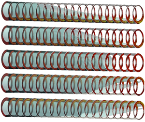
Figure 13 shows results for a flow with  $(e,Re,b,\hat {\mu }_2/\hat {\mu }_1)=(0.46,805.69,5.37,1.08)$. Figures 13(a), 13(b), 13(c) and 13(d) show respectively: the averaged concentration front view, bottom view, front view of the first section of annulus and front view of the first section of the experiment, at
  $\hat {t}=5$ s. The front slumps towards the bottom but the top of the front is found just above the bottom of the annulus, again signifying competition. The tip of the front is dispersive due to small density difference, near-identical viscosities and high
  $Re$. We see that there is a thin layer trapped in bottom side of the annulus which is slowly displaced as the main front advances. The residual layer is asymmetric and is unstable/wavy, as it is generated at the front. Compared to the previous example, the eccentricity is more modest, the value of
  $b$ is fairly insignificant and the Reynolds number increased. The most wavy part of the residual layer is near the front and we see that this decays upstream. For the flow of figure 13 there is no distinct stratification of the fluids in the upper part of the annulus (instead a very dispersive front). Thus, common inertial wave-like instability mechanisms such as Kelvin–Helmholtz may be discounted.

Figure 13. For  $(e,Re,b,\hat {\mu }_2/\hat {\mu }_1)=(0.46,805.69,5.37,1.08)$, EXP 165. At
  $t=5$ s: (a) depth-averaged concentration front view, (b) height-averaged concentration bottom view, (c) height-averaged concentration bottom view of annulus first section and (d) shows the bottom view picture from the experiment. At
  $t=7$ s: (e) depth-averaged concentration front view, ( f) height-averaged concentration bottom view and (g) height-averaged concentration bottom view of annulus second section. At
  $t=15$ s: (i) depth-averaged concentration front view, (j) height-averaged concentration bottom view and (k) shows the bottom view picture from the experiment. Black dashed line shows
  $\bar {C}_y=0.5$.
Figures 13(e), 13( f) and 13(g) show the averaged concentration front view, bottom view, and front view of the second section of annulus at  $\hat {t}=7$ s. We can clearly observe the slumping dispersive flow similar to
  $\hat {t}=5$ s. The corresponding experimental result did not clearly show a residual channel in this last section of the annulus. Figures 13(h) and 13(i), show the averaged concentration front view and bottom view of the entire annulus at
  $\hat {t}=15$ s. Figure 13(j,k) shows the front view of the last section, for simulation and experiment, also at
  $\hat {t}=15$ s. The front cannot be easily identified as the flow is highly dispersive. The unstable wavy residual layer, extends along almost half of the total length.
3.2. Steady and unsteady flows
A key descriptor of primary cementing displacement flows is whether the displacement is ‘steady’ or ‘unsteady’. In an idealized setting, a steady displacement means that the front advances steadily along the annulus, at the same (mean pumping) speed at all points around the annulus. This state is well defined and predictable in reduced models of the displacement (Pelipenko & Frigaard Reference Pelipenko and Frigaard2004a,Reference Pelipenko and Frigaardb; Carrasco-Teja et al. Reference Carrasco-Teja, Frigaard, Seymour and Storey2008), where one can even find analytical solutions in special circumstances. For a Newtonian–Newtonian displacement the solutions depend only on  $b$,
$b$,  $e$,
$e$,  $\hat {\mu }_2/\hat {\mu }_1$ and the annulus inclination (fixed here). In Renteria & Frigaard (Reference Renteria and Frigaard2020) we have seen that horizontal displacements are rarely this ‘clean’: gap-scale and azimuthal dispersive secondary flows smear the interface and imaging artefacts both limit the range of
  $\bar {C}_y$ reliably measurable and make front velocity calculations vulnerable to errors. Consequently, in Renteria & Frigaard (Reference Renteria and Frigaard2020) we used threshold values of
  $\hat {W}_f(\bar {C}_y)$ lying well within the reliably measurable range of our experimental system and classified steady flows by the threshold
 \begin{equation} \hat{W}_f(\bar{C}_y=0.3)-\hat{W}_f(\bar{C}_y=0.7) \leq 0.1 \hat{W}_0, \end{equation}
and unsteady flows otherwise.
As we have seen in our simulations, we are able to capture very similar secondary flows as in the experiments. Additionally, having eliminated imaging issues, we are able to differentiate the displacement height-averaged concentration profiles to calculate  $\hat {W}_f(\bar {C}_y)$ at higher resolution than in the experiments and over the full range of
  $\bar {C}_y$. Thus, a different criterion than (3.1) could be adopted. However, that is not the aim here. Instead, we wish to first verify that the simulations reproduce the experiments to the degree to which they have already been classified. If so, in many ways the simulations are a better tool for a deeper and more detailed investigation of the flow structure.
Figure 14 compares classification of the 3-D simulations using (3.1) compared to the same classification of the experiments from Part 1. Note that, in Part 1, this classification was applied only to slumping flows and only to a subset of the experiments for which the image quality was sufficiently high. The top side displacements are in general unsteady as there is no limiting mechanism. We see that the results are in a close agreement except two cases with large eccentricity  $e=0.73$. In addition, all the cases with high value of viscosity ratio (
 $\hat {\mu }_2/\hat {\mu }_1\geq 10$) are classified as steady.

Figure 14. Steady/unsteady classifications for slumping displacements according to the threshold. Comparison between experimental data (filled symbols) and the corresponding 3-D simulations (larger white symbols). The colour bar represents the viscosity ratio ( $\hat {\mu }_2/\hat {\mu }_1$) of the experiment.
The following results, in figures 15–17 present steady and unsteady displacement flows arising from different balances and mechanisms, exploring transitional regimes. Figure 15(a) shows the height-averaged concentration  $\bar {C}_y$ at successive times for
  $(e,Re,b,\hat {\mu }_2/\hat {\mu }_1)=(-0.07,304.55,69.08,1.50)$, experiment 309. Each curve is computed from the concentration map at a given time and thus suggests the shape of the front. In this case, both the marginally wider gap at the bottom and the small positive
  $b$, promote slumping of the front to the bottom of the annulus and the viscosity ratio is close to
  $1$, so has little effect. Figure 15(b) shows the normalized front velocity computed by differentiating between curves at fixed
  $\bar {C}_y$ at long times in figure 15(a). This flow (figure 15) is classified as unsteady using the classification (3.1). An interesting comparison here is with the (unsteady) top side displacement of figures 8 and 9, which have identical
  $e$, similar
  $|b|$ but negative and also
  $O(1)$ viscosity ratio.

Figure 15. For  $(e,Re,b,\hat {\mu }_2/\hat {\mu }_1)=(-0.07,304.55,69.08,1.50)$, EXP 309. (a) Height-averaged concentration evolution in time (
 $\bar {C}_y(\hat {x},\hat {t})$) and (b) dimensionless fully developed front velocities (
 $\hat {W}_f/\hat {W}_0$) for different height-averaged concentrations (
 $\bar {C}_y$).
Figure 16 shows the slumping flow of figure 15 in more detail at  $\hat {t}=25$ s. Figure 16(a) shows the iso-surface
  $C=0.5$, illustrating the slumping flow and dispersive spikes in top and bottom annular gaps. The rest of figure 16 presents the secondary flows within cross-sections at distances positioned upstream and downstream of the front. As previously, the grey scale indicates the strength of axial velocity (
 $\hat {W}/\hat {W}_0-1$), the contours are streamlines of the flow within each
  $(x,y)$-plane and these contours are coloured with the local axial component of vorticity. The blue lines show the iso-line
  $C=0.5$, the position of the interface. Just upstream of the front (figure 16b) we see the displacement is near complete and is also nearly symmetric (i.e. L-R). The denser fluid is pushing the lighter fluid to drain upwards. Thus we see the associated streamlines driving the secondary flow upwards on each wall. Slightly further downstream (figure 16c–e), 2 strong vorticity regions are found lower in the flow, associated with pushing the lighter fluids upwards along the walls. Away from the walls it is notable that the iso-surface
  $C=0.5$ is essentially stratified. Although we see recirculatory streamlines in wide gap, the largest vorticity is generated at the interfaces of the wall layers, presumably due to buoyancy gradients. We note that this is also localized azimuthally at approximately the position where
  $C=0.5$. In the sequence of figure 16(b–e), the relative strength of the secondary flow to the mean flow is largest in figure 16(d), just as the interface enters the wide gap at the bottom. The strength of secondary flows in this example is similar but smaller than that in figure 9, but in many ways the flow structure appears very similar, except slumping to the bottom instead of top.

Figure 16. Azimuthal flow near the interface for  $(e,Re,b,\hat {\mu }_2/\hat {\mu }_1)=(-0.07,304.55,69.08,1.50)$, EXP 309 at
  $\hat {t}=25$ s. (a) Iso-surface
  $C=0.5$, streamlines at: (b)
  $\hat {x}=2.5$ m, (c)
  $\hat {x}=3.5$ m, (d)
  $\hat {x}=4$ m and (e)
  $\hat {x}=4.5$ m. Streamlines are coloured by vorticity (
 $\omega _x$). Blue line shows the iso-line
  $C=0.5$ and grey scale represents
  $\hat {W}/\hat {W}_0-1$.
The next displacement was performed at near-identical conditions with the same fluid pairing, but in a positively eccentric annulus: parameters  $(e,Re,b,\hat {\mu }_2/\hat {\mu }_1)=(0.46,299.12,71.74,1.48)$. The eccentricity slows motion along the narrow lower part of the annulus and this experiment (experiment 313) is classified as steady. The height-averaged concentrations and front velocities are qualitatively similar to those of figure 6. Figure 17(a) illustrates the iso-surface
  $C=0.5$ at
  $t=25$ s. We can see that the length of slumping front is smaller compared to figure 16(a). The spikes also appear to extend a shorter distance. Figure 17(b–e) shows more detail of the slumping flow within cross-sections at distances positioned upstream and downstream of the front. The most interesting feature is that the secondary flows are asymmetric and significantly more so than in figure 16(b–e) and secondary flows are stronger than the previous example. Similar to previous cases, there is strong vorticity near the interface and 2 sets of recirculating streamlines near the inner and outer walls to squeeze and push the displaced fluid upward. It appears that the steadiness of the front in this example comes from the azimuthal flow promoted by the wider top gap (balancing the positive buoyancy) and the smaller gap at the bottom (slowing the stratification), i.e. only the eccentricity has changed. However, the asymmetry indicates that this balance may not be stable.

Figure 17. Azimuthal flow near the interface for  $(e,Re,b,\hat {\mu }_2/\hat {\mu }_1)=(0.46,299.12,71.74,1.48)$, EXP 313 at
  $\hat {t}=25$ s. (a) Iso-surface
  $C=0.5$, streamlines at: (b)
  $\hat {x}=2.25$ m, (c)
  $\hat {x}=2.75$ m, (d)
  $\hat {x}=3.25$ m and (e)
  $\hat {x}=3.5$ m. Streamlines are coloured by (
 $\omega _x$). Blue line shows the iso-line
  $C=0.5$ and grey scale represents
  $\hat {W}/\hat {W}_0-1$.
3.3. Parametric effects
Although the experiments in Renteria & Frigaard (Reference Renteria and Frigaard2020) cover a wide range of the dimensionless parameters, some effects are difficult to study in isolation due to experimental constraints. Here, we explore in more detail these effects.
3.3.1. Effect of eccentricity
To study the effect of eccentricity ( $e$), we fix the parameters
  $(Re,b, \hat {\mu }_2/\hat {\mu }_1)=(148.99,0.95,0.87)$ (modelled on experiment 125) and change the eccentricity incrementally from
  $-0.4$ to
  $0.8$. The flow has been chosen as it has moderate viscosity ratio and very small positive
  $b$. Figure 18 shows the iso-surface
  $C=0.5$ for these parameters. It shows that the slumping displacement changes from slumping to top side displacement by increasing the eccentricity, with minimal influence of
  $b$. Therefore, the flow has a tendency to displace in the widest gap. We recall that at large Péclet number the fluids are mostly advected and hence the faster flowing regions determine where the front will advance.

Figure 18. Snapshots of displacement flow for different eccentricities for  $(Re,b, \hat {\mu }_2/\hat {\mu }_1)=(148.99,0.95,0.87)$ at
  $\hat {t}=8$ s. Colour map of equally spaced slices represents concentration of the displacing fluid and the blue shaded region shows the iso-surface
  $C = 0.5$. Dimensionless axial velocity (
 $\hat {W}/\hat {W}_0$) is shown on slices and the colour map presents its magnitude.
Investigating these sorts of examples is difficult experimentally at large values of  $e$, positive or negative, as errors in setting the gap are most significant. Equally, it is time consuming to set and adjust the eccentricity accurately for a single experimental fluid combination (hence, in Part 1, we performed experiments over 3 fixed eccentricities only). Some ripples can be seen for
  $e=-0.4$ to
  $0.4$ and they vanish for higher
  $e$. Ripples are caused by steepness of the front and potentially the inertial effect of moderate
  $Re$; they vanish when the flow is more stratified and the eccentricity effect is dominant. Recall also our earlier figure 17 and the asymmetries observed as the front steepens. The normalized axial velocity (
 $\hat {W}/\hat {W}_0$) is also shown in figure 18 on cross-sections equally spaced along the annulus. The wide gap has the highest velocity for small
  $b$ and moderate viscosity ratio. For very high eccentric cases (
 $e\geq 0.6$) barely any flow can be seen in the narrow gap.
Figure 19 shows the variation of averaged concentrations of the displacing fluid, computed by averaging across the gap and along the annulus, on both the top and bottom of the annulus ( $\theta =0,{\rm \pi}$). These are for the same parameters as figure 18 and at the same time. This shows that there is an eccentricity at which the flow switches from top side to slumping, characterized by the larger gap-averaged concentration; e.g. in this case
  $e_{transition}\approx 0.15$. If we inspect the gap-scale velocity in figure 18 we can see that for this modest viscosity ratio there will always be a tendency to disperse on the annular-gap scale. The connection between the transition in averaged concentrations and occurrence of a steady state displacement is also not clear.

Figure 19. Variation with  $e$ of the concentration (
 $\bar {C}$) averaged across the gap and along the annulus on top and bottom sides of the annulus, for
  $(Re,b, \hat {\mu }_2/\hat {\mu }_1)=(148.99,0.95,0.87)$ at
  $\hat {t}=8$ s.
3.3.2. Effect of viscosity ratio
In Renteria & Frigaard (Reference Renteria and Frigaard2020) we found that the viscosity ratio was of secondary importance in determining the flow behaviour, i.e. less relevant than eccentricity and buoyancy. This contrasts with the more prominent role of viscosity ratio in the asymptotic theory developed by Carrasco-Teja et al. (Reference Carrasco-Teja, Frigaard, Seymour and Storey2008). Partly this different emphasis arises because, even though a broad range of  $\hat {\mu }_2/\hat {\mu }_1$ was studied in Renteria & Frigaard (Reference Renteria and Frigaard2020), the variations were still limited by the fluids used. For example, variation of viscosity is often accompanied by density change so that
  $b$ and
  $\hat {\mu }_2/\hat {\mu }_1$ are not independently varied. The simulations here have no such issue.
The effect of viscosity ratio ( $\hat {\mu }_2/\hat {\mu }_1$) is shown in figure 20 for fixed parameters
  $(e,Re,b)=(0.46,40.14,518.51)$ (modelled on experiment 312 with
  $\hat {\mu }_2/\hat {\mu }_1=1.5$) at
  $\hat {t}=140$ s. The blue shaded region shows the iso-surface
  $C=0.5$. The normalized axial velocity (
 $\hat {W}/\hat {W}_0$) is shown on equally spaced cross-sections and coloured by its magnitude. In these simulations the flows tend to slump as
  $b$ is very large. However, the displacement front elongates less as viscosity ratio (
 $\hat {\mu }_2/\hat {\mu }_1$) is increased. This promotes steadiness of the displacement front, in the sense of § 3.2.

Figure 20. Snapshots of displacement flow for different viscosity ratios for  $(e,Re,b)=(0.46,40.14,518.51)$ at
  $\hat {t}=140$ s; (a)
  $\hat {\mu }_2/\hat {\mu }_1=0.5$, (b)
  $\hat {\mu }_2/\hat {\mu }_1=1$, (c)
  $\hat {\mu }_2/\hat {\mu }_1=1.5$, (d)
  $\hat {\mu }_2/\hat {\mu }_1=2.5$ and (e)
  $\hat {\mu }_2/\hat {\mu }_1=5$. Colour map of equally spaced slices represents concentration of the displacing fluid and the blue shaded region shows the iso-surface
  $C=0.5$. Dimensionless axial velocity (
 $\hat {W}/\hat {W}_0$) is shown on slices and the colormap presents its magnitude.
Both far upstream and downstream of the front the wide gap has the highest velocity, as expected. We can also see that the flow is fast on the narrow side near the interface. However, figure 20(a) shows that stratification appears to drive the axial flow forward just under the interface, e.g. see figure 20(a,b). It seems that the fast wide side flow from upstream is pushed downwards under the interface. For these lower values of  $\hat {\mu }_2/\hat {\mu }_1$ the stream of faster moving displacing fluid extends to the bottom of the annulus; hence, the interface continues to slump and extend. For the smallest
  $\hat {\mu }_2/\hat {\mu }_1$ the stream of displacing fluid in the advancing front causes the velocity above the interface to slow considerably (figure 20a). As
  $\hat {\mu }_2/\hat {\mu }_1$ is increased the fluid upstream of the front resists the advancement on the narrow side, the front steepens and the stream under the interface widens. A more uniform azimuthal distribution of axial velocities is found (figure 20c,d). The frontal region is also associated with strong secondary flows (such as discussed with figure 7 earlier). This mechanism results in the type of flows that we have termed steady.
Figure 21 shows the variation of averaged concentrations of the displacing fluid, computed by averaging across the gap and along the annulus, on both the top and bottom of the annulus ( $\theta =0,{\rm \pi}$). These are for the same parameters as figure 20 and at the same time. This shows that front elongates less as viscosity ratio (
 $\hat {\mu }_2/\hat {\mu }_1$) is increased for this slumping flow. A high value of the viscosity ratio results in a more uniform displacement front and promotes steady displacement.

Figure 21. Variation with  $\hat {\mu }_2/\hat {\mu }_1$ of the concentration (
 $\bar {C}$) averaged across the gap and along the annulus on the top and bottom of the annulus, for
  $(e,Re,b)=(0.46,40.14,518.51)$ at
  $\hat {t}=140$ s.
Figure 22 illustrates the effect of viscosity ratio on the displacement efficiency. It shows the area-averaged concentration  $\bar {C}$, computed over the full cross-section at each axial position
  $\hat {x}$, at two times: at
  $\hat {t}=120,\ 200$ s. The data are taken from the computations of figure 20. We can see that the higher viscosity ratio has reduced the slope of
  $\bar {C}$. Furthermore, the shape of the front at
  $\hat {\mu }_2/\hat {\mu }_1=2.5,\ 5$ is approximately unchanged in time, resulting in a successful displacement. We will further explore this example below.

Figure 22. Average concentration ( $\bar {C}$) variation along the well for different viscosity ratios for
  $(e,Re,b)=(0.46,40.14,518.51)$ at (a)
  $\hat {t}=140$ s and (b)
  $\hat {t}=200$ s. Viscosity ratios are
  $\hat {\mu }_2/\hat {\mu }_1=0.5,\ 1.5,\ 2.5,\ 5$.
3.4. Annular displacements modelled in one dimension
Reduced models are essential for industrial process design. Although here we have effectively used 3-D simulations to study laboratory-scale experiments, the annulus length is still very small with respect to those in the field. Simulating a full wellbore at acceptable numerical resolutions remains currently out of reach. The wellbore length increases not only the number of mesh cells proportionately, but also the time of the simulation (displacement flow). Since displacement fronts are complex, may disperse or not, may leave long residual layers, etc. it is not clear that one could universally apply adaptive meshing to pick out these features. At least this is a complex challenge for the future.
Thus, we return to reduced models. In Part 1, we used the (laminar) computations of Maleki & Frigaard (Reference Maleki and Frigaard2017) and worked within the theoretical framework of Carrasco-Teja et al. (Reference Carrasco-Teja, Frigaard, Seymour and Storey2008). The simulations performed used a 2DGA model, which ignores inertia and is a narrow-gap approximation. The main discrepancies between experimental results and the 2DGA results in Part 1 came from several mechanisms of dispersion and potentially from neglected inertial effects. In particular, the 2DGA has only radially homogeneous concentrations and velocities. Although azimuthal secondary flows are present, the gap-scale dispersion that has been so evident here, is absent. A long term goal is to include such effects in the 2DGA approach, but we first explore a simpler approximate approach.
3.4.1. Advective effects
In Renteria & Frigaard (Reference Renteria and Frigaard2020), we did explore evolution of the area-averaged concentration  $\bar {C}_y(\hat {x},\hat {t})$, in an effort to describe spreading of the front along the annulus. We were hampered by inconsistent data resolution and imaging artefacts at high and low
  $\bar {C}_y$. We return to this task now computationally. Figure 23 shows spatio-temporal maps of averaged concentration (
 $\bar {C}_y(\hat {x},\hat {t})$) for fixed parameters
  $(e,Re,b)=(0.46,40.14,518.51)$ and different viscosity ratios, similar to figure 20. The black and grey broken lines show
  $\bar {C}_y(\hat {x},\hat {t})=0.3$ and
  $0.7$, respectively. The slopes of these lines are the front velocities for
  $\bar {C}_y(\hat {x},\hat {t})=0.3$ and
  $0.7$. As the viscosity ratio is increased these slopes become progressively parallel e.g. figure 23(d), resulting in a steady displacement. Of course, there is a question of threshold to define steadiness, as some spreading of the concentration field is also evident in figure 23(d).

Figure 23. Spatio-temporal map of averaged concentration  $\bar {C}_y(\hat {x},\hat {t})$ for
  $(e,Re,b)=(0.46,40.14,518.51)$; (a)
  $\hat {\mu }_2/\hat {\mu }_1=0.5$, (b)
  $\hat {\mu }_2/\hat {\mu }_1=1.5$, (c)
  $\hat {\mu }_2/\hat {\mu }_1=2.5$ and (d)
  $\hat {\mu }_2/\hat {\mu }_1=5$. Dashed black line and dashed grey line show
  $\bar {C}_y(\hat {x},\hat {t})=0.3$ and
  $0.7$, respectively.
Figure 24 shows the developed front velocities, normalized with the mean velocity ( $\hat {W}_f/\hat {W}_0$), as a function of averaged concentration for the same parameters as figure 23. We see that the higher viscosity ratio reduces the variation of front velocity and increase the steadiness of the flow. For high enough viscosity ratio, the front velocity converges to the mean flow velocity, see figure 24(d). Using these front velocities we now construct the advective flux
 \begin{equation} \hat{q}(\bar{C}_{adv,y}) = \int_0^{\bar{C}_{adv,y}} \hat{W}_f(s)\,\textrm{d}s, \end{equation}
and integrate the following equation:
 \begin{equation} \frac{\partial \bar{C}_{adv,y}}{\partial \hat{t}}+\frac{\partial }{\partial \hat{x}} \hat{q}(\bar{C}_{adv,y})=0. \end{equation}
A total variational diminishing method with Min-Mod limiter is used to solve the 1-D conservation equation (3.3). The quantity  $\bar {C}_{adv,y}$ corresponds to the advected concentration, i.e. that which would result from transport due to the long-time/developed front velocity.

Figure 24. Dimensionless fully developed front velocities ( $\hat {W}_f/\hat {W}_0$) for different height-averaged concentrations (
 $\bar {C}_y$) for
  $(e,Re,b)=(0.46,40.14,518.51)$; (a)
  $\hat {\mu }_2/\hat {\mu }_1=0.5$, (b)
  $\hat {\mu }_2/\hat {\mu }_1=1.5$, (c)
  $\hat {\mu }_2/\hat {\mu }_1=2.5$ and (d)
  $\hat {\mu }_2/\hat {\mu }_1=5$.
Figure 25 shows the advected concentration evolution in time for two of the viscosity ratios (figure 25a,c). In figure 25(b,d) we plot the spatio-temporal maps of  $\bar {C}_{y}-\bar {C}_{adv,y}$. The dashed line shows
  $\bar {C}_{y}=0.5$. We first observe that the over much of the domain the colour map is very close to zero, suggesting that
  $\bar {C}_{adv,y}$ does capture much of the variation in
  $C$. However, at later times the highest contours of
  $\bar {C}_{y}-\bar {C}_{adv,y}$ appear localized in an expanding strip around the black dashed line. As this strip is close to
  $\bar {C}_y=0.5$, it seems likely that this region is dominated by diffusive mechanisms. However, the spreading seems limited i.e. we have constant contouring outside of this strip in figure 25(b,d), which seems to have a ‘edge’. Another observation is that the darker regions where initial effects are not captured, possibly since
  $\bar {C}_{adv,y}$ uses late-time values of the front velocity.

Figure 25. Parameters  $(e,Re,b)=(0.46,40.14,518.51)$: (a)
  $\hat {\mu }_2/\hat {\mu }_1 = 1.50$, advective concentration
  $\bar {C}_{adv,y}$; (b)
  $\hat {\mu }_2/\hat {\mu }_1 = 1.50$, spatio-temporal map of
  $\bar {C}_{y}-\bar {C}_{adv,y}$; (c,d) as (a,b) but with
  $\hat {\mu }_2/\hat {\mu }_1 = 5$. The black dashed line shows
  $\bar {C}_y=0.5$.
3.5. Bulk axial diffusion
Having seen that  $\bar {C}_{adv,y}$, captures only part of the front spreading mechanisms, we resort instead to a simpler approach to quantify the bulk effects on
  $\bar {C}_y$, We follow the approach in Renteria & Frigaard (Reference Renteria and Frigaard2020) in plotting profiles of
  $\bar {C}_y$ against the diffusive similarity variable
  $(\hat {x}-\hat {W}_0\hat {t})/\sqrt {\hat {t}}$. This choice removes the mean advection. Figure 26 shows the results of doing this for the same parameters as figure 24. We can see that data collapse well against the diffusive similarity variable, as we have seen in experiments, although better for higher viscosity ratio, i.e. closer to steady flows.

Figure 26. The result of plotting  $\bar {C}_y(\hat {x},\hat {t})$ against
  $(\hat {x}-\hat {W}_0\hat {t})/\sqrt {\hat {t}}$ for
  $(e,Re,b)=(0.46,40.14,518.51)$; (a)
  $\hat {\mu }_2/\hat {\mu }_1=0.5$, (b)
  $\hat {\mu }_2/\hat {\mu }_1=1.5$, (c)
  $\hat {\mu }_2/\hat {\mu }_1=2.5$ and (d)
  $\hat {\mu }_2/\hat {\mu }_1=5$. The solid red line shows a fit using the complementary error function, with diffusivity: (a)
  $\hat {D}=0.0112$ m
 $^2$ s
 $^{-1}$, (b)
  $\hat {D}=0.0044$ m
 $^2$ s
 $^{-1}$, (c)
  $\hat {D}=0.0022$ m
 $^2$ s
 $^{-1}$ and (d)
  $\hat {D}=0.0008$ m
 $^2$ s
 $^{-1}$.
We approximate each single curve of the collapsed data with a complementary error function, fitting a diffusivity using a nonlinear least squares method. We then average the diffusivity for each experiment over the values fitted for each timeframe: typically the time frame values are within 10 % of the mean. Values of diffusivity  $\hat {D}$ are given for each example in figure 26. From this figure and figure 24 earlier, we see that higher viscosity ratio increases the steadiness of the flow, decreases
  $\Delta \hat {W}_f$ and the diffusivity
  $\hat {D}$. We have repeated this calculation for the same slumping displacements as in Part 1. Figure 27 shows the normalized front velocity difference
  $\Delta \hat {W}_f/(\hat {W}_0)$, plotted against the dimensionless bulk diffusivity coefficient, computed as in figure 26. These clearly correlate, as also reported from our experimental observations in Renteria & Frigaard (Reference Renteria and Frigaard2020). The normalized macroscopic diffusion coefficient for cases with intermediate eccentricity
  $e=0.46$ are
  $\lesssim$1, whereas for
  $e=0.73$ and
  $e=-0.07$ the values spread along a wider interval. The cases with the highest viscosity ratio also present the smallest coefficient, independently from the eccentricity. As explained in § 3.3.2, a high viscosity ratio reduces stratification of the interface by slowing the motion in the narrow bottom gap.

Figure 27. The result of plotting  $\hat {D}/{\rm \pi} \hat {r}_o\hat {W}_0$ against
  $\Delta \hat {W}_f/\hat {W}_0$ for selected slumping classified simulations:
  $e = -0.07$ circle;
  $e = 0.46$ square;
  $e = 0.73$ triangle. The colour bar represents the viscosity ratio (
 $\hat {\mu }_2/\hat {\mu }_1$) of the simulation.
Figure 28 compares the experimental and 3-D normalized front velocity differences and bulk diffusivity coefficients. The front velocities from the experiment were computed as  $\hat {x}_f/\hat {t}$ for each concentration, whereas the 3-D front velocities came from differentiating the profiles of
  $\bar {C}_y$. In both cases, references values are taken at long times in the simulation/experiment. The front velocities agree well albeit with some variations, especially for
  $e=-0.07$.

Figure 28. (a) Value of  $\Delta \hat {W}_f/\hat {W}_0$ for experiments and 3-D simulations and (b) dimensionless diffusion value
  $\hat {D}/{\rm \pi} \hat {r}_o\hat {W}_0$ for selected slumping classified experiments.
  $e = -0.07$ in red circle,
  $e = 0.46$ in green square and
  $e = 0.73$ in blue upside-down triangle.
Likewise, in figure 28(b), the dimensionless bulk diffusion coefficient compares well with the experimental. The experimental bulk diffusivities in Renteria & Frigaard (Reference Renteria and Frigaard2020) were estimated by making a collapse of the average concentrations  $\bar {C}_y$ (taken from the images) against the diffusive similarity variable
  $(\hat {x}-\hat {W}_0\hat {t})/\sqrt {\hat {t}}$ and then making an eye fit. The 3-D model results were computed objectively as concentrations and then fitted numerically as described. Although the methods are different, the agreement is fair and importantly the same trends are reproduced. Note that both, the difference in front velocities and the macroscopic diffusion coefficient display the non-monotonic behaviour shown in Renteria & Frigaard (Reference Renteria and Frigaard2020): the lowest values are found for the intermediate eccentricity (
 $e=0.46$) and the highest for displacements close to concentric (
 $e=-0.07$).
The source of the bulk diffusion may be the result of several mechanisms, yet at first glance it appears to be mainly gravitationally driven, as in the model of Carrasco-Teja et al. (Reference Carrasco-Teja, Frigaard, Seymour and Storey2008). However, the magnitude of  $\hat {D}$ certainly contains contributions from various local effects happening near the interface, as exhaustively described throughout this work. The interface stratifies for high
  $|b|$ values and becomes steeper with increasingly high viscosity ratios. Eccentricity can resist the stratification in a slumping displacement and even result in something that appears steady. Nevertheless, too much eccentricity either promotes the flow in the wider top side or creates residual layers at the narrow (bottom) side. Thus, the non-monotonic trend in the magnitude of
  $\hat {D}$ with the eccentricity is not unexpected. It appears, however, that the role of buoyancy in this type of horizontal annular displacements is more complex than previously suggested in Carrasco-Teja et al. (Reference Carrasco-Teja, Frigaard, Seymour and Storey2008), where buoyancy acts only to determine the axial length of the slumping front.
4. Discussion and conclusions
In this paper we have shown that 3-D simulations are able to capture the dominant features of eccentric annular displacement flows quantitatively, e.g. see figures 5 and 8. Over wide ranges of parameters covering the experiments in Part 1, the simulations give very close matches in classifying flows (top/slumping, steady/unsteady). Equally, the simulations are effective at predicting other features such as narrow side residual layers. This is important practically as it is these descriptors that are used industrially to understand whether a particular cementing design might be effective or problematic.
The simulation results reveal a complex flow structure that is simply not visible in our experiments. For example, it is hard to visualize thin residual wall layers draining along the sides of the annulus near the front and capturing secondary flow features would be extremely challenging. Therefore, a key contribution of our paper is to validate the use of simulations as a tool. We can now directly investigate dispersive and 3-D structures, e.g. recirculatory vortices, spikes, wall layers and azimuthal flows, We can now do this in a more systematic way than has been possible here. Some other insights are as follows.
Buoyancy acts to stratify the flow and competes with eccentricity to control the leading order behaviour of the interface. It also acts to drive heavy fluids down and light fluids up, within the secondary flows evident in the cross-sections. These secondary flows are driven by the mean flow and by  $b$: smaller
  $|b|$ reduces the magnitude of the secondary flow. Characteristically, for moderate
  $|b|$ the iso-concentration lines tend to stratify with gravity in the centre of the annular space, where it is wide, but near the walls residual fluid layers persist. Density gradients act to squeeze the residual fluid in the direction of buoyancy as viscous stresses drag the fluid downstream (predominantly). Higher viscosity in the displacing fluids leads to thicker residual layers and slower azimuthal removal. Buoyancy is not, however, effective at driving the fluids azimuthally at the top/bottom of the annulus. In particular, the viscosity ratio seems to be important in displacing the narrow side at the bottom of the annulus, (for
  $e>0$). The small gap slows the displaced fluid flow and front advancement in a slumping flow. The front then steepens, the spreading is reduced and we have regimes of ‘steady’ displacement. However, this balance appears delicate. We have seen that severe eccentricity or an insufficiently large viscosity ratio result in long residual layers on the lower narrow side, often sinuous and unstable.
What of simpler models? The results of our simulations and the experiments of Renteria & Frigaard (Reference Renteria and Frigaard2020) globally agree with the results of the 2DGA model (Carrasco-Teja et al. Reference Carrasco-Teja, Frigaard, Seymour and Storey2008; Maleki & Frigaard Reference Maleki and Frigaard2017), in predicting qualitative features, but also succeed in resolving dispersive effects fully. Although there is an underlying competition between buoyancy and eccentricity, it is worth pointing out that the asymptotic ‘lubrication’ model of Carrasco-Teja et al. (Reference Carrasco-Teja, Frigaard, Seymour and Storey2008) is incomplete. In it, large buoyancy  $|b| \gg 1$ determines the axial length scale of slumping and whether developed flows are steady or unsteady is then determined by eccentricity and rheology. However, as is common in most thin-film approaches, the initial classification of a slumping flow is assumed. As we have seen, the transition between slumping and top side regimes is itself a competition between
  $(e,b)$ and other variables
  $(Re,\hat {\mu }_2/\hat {\mu }_1)$, to a lesser extent. Secondly, even in slumping flows we have seen many instances of narrow side residual layers. These are also seen in the 2DGA model, but are missing from the lubrication theory. In the last part of this paper we have explored whether a simpler 1-D description would be viable. It seems that neither an advective description nor a diffusive description fully captures the observed bulk spreading behaviour, although both give some quantitative information useful for estimation.
Lastly, the notion of a steady displacement is key to simpler models of cementing (Carrasco-Teja et al. Reference Carrasco-Teja, Frigaard, Seymour and Storey2008; Maleki & Frigaard Reference Maleki and Frigaard2017). Although we see steepening of the front and have classified displacements as ‘steady’ or unsteady, dispersion means that even the steady displacement flows have frontal regions that extend with time. We have adopted a pragmatic approach to defining ‘steady’ flows, via a heavily thresholded criterion (3.1). This is robust for our simulations and experiments, but, in different set-ups, the notion of a long time would need better specification. Certainly it means to avoid initial transients, but in a slowly evolving flow, when exactly should we evaluate the flow? Equally, we note that steady front propagations such as that in figure 6(b) may satisfy (3.1), but still have significant residual fluid layers. Despite these issues, we still feel that the notion of a steady displacement remains useful. Not only are such flows dynamic features of reduced models such as those of Carrasco-Teja et al. (Reference Carrasco-Teja, Frigaard, Seymour and Storey2008) and Maleki & Frigaard (Reference Maleki and Frigaard2017), but it is also a powerful concept to describe what an ideal flow should look like. The difficulty is how to understand this in the presence of significant dispersion, i.e. how to identify a steady flow. Interestingly, similar difficulties are faced in fully turbulent annular displacement flows, where Taylor dispersion is present, where a differential velocity criterion has been applied with some success (Maleki & Frigaard Reference Maleki and Frigaard2020).
Acknowledgements
The authors also express their gratitude to the Mexican National Council for Science and Technology (SENER-CONACYT) for financial support (AR).
Funding
This research has been carried out at the University of British Columbia (UBC). Financial support for the study was provided by NSERC and Schlumberger through CRD Project No. 516022-17. This research was also enabled in part by infrastructure provided from UBC Advanced Research Computing (ARC) (https://arc.ubc.ca). Experimental infrastructure was funded by the Canada Foundation for Innovation and the BC Knowledge Development Fund, grant number CFI JELF 36069. This funding is gratefully acknowledged.
Declaration of interests
The authors report no conflicts of interest.


