


1. Introduction
Immiscible two-phase displacement in permeable media has drawn extensive research attention due to its importance in secondary and tertiary oil recovery processes (Lake Reference Lake1989). However, many petroleum-bearing underground geological formations exist in the form of layers, which poses great technical challenges for the economical recovery of original oil due to early breakthrough (Sheng Reference Sheng2013; Bahadori Reference Bahadori2018). Injecting gas (e.g. carbon dioxide) or liquid (e.g. water) into a subsurface system with permeability variations often leads to the preference of the injected flow into one of the layers, and whether high or low permeability depends on the fluid properties such as viscosity, interfacial tension, density, buoyancy and solubility; the properties of porous media such as surface wettability, porosity and permeability; and the operational conditions such as the injection rate. In order to optimise the gas or liquid flooding operations and thus improve oil recovery, it is crucial to understand the fundamentals of two-phase displacement in porous media with permeability contrast.
Extensive works have been devoted to understanding two-phase displacement mechanisms from experimental (Lenormand, Touboul & Zarcone Reference Lenormand, Touboul and Zarcone1988; Zhang et al. Reference Zhang, Oostrom, Wietsma, Grate and Warner2011b; Zhao, MacMinn & Juanes Reference Zhao, MacMinn and Juanes2016; Hu et al. Reference Hu, Patmonoaji, Zhang and Suekane2020), theoretical (Chatzis & Dullien Reference Chatzis and Dullien1983; Laidlaw & Wardlaw Reference Laidlaw and Wardlaw1983; Sorbie, Wu & McDougall Reference Sorbie, Wu and McDougall1995; Al-Housseiny, Tsai & Stone Reference Al-Housseiny, Tsai and Stone2012; Al-Housseiny, Hernandez & Stone Reference Al-Housseiny, Hernandez and Stone2014; Zheng, Kim & Stone Reference Zheng, Kim and Stone2015; Zheng, Rongy & Stone Reference Zheng, Rongy and Stone2015) and numerical (Liu et al. Reference Liu, Valocchi, Kang and Werth2013; Sun, Kharaghani & Tsotsas Reference Sun, Kharaghani and Tsotsas2016; Chen et al. Reference Chen, Valocchi, Kang and Viswanathan2019) perspectives. Lenormand et al. (Reference Lenormand, Touboul and Zarcone1988) experimentally studied a non-wetting fluid displacing a wetting fluid (i.e. drainage) in a micromodel and found that the competition between capillary and viscous forces creates an instability of the advancing front, leading to three different displacement regimes, namely viscous fingering, capillary fingering and stable displacement, which were mapped on a phase diagram of viscosity ratio versus capillary number. Later, the phase diagram was improved by Zhang et al. (Reference Zhang, Oostrom, Wietsma, Grate and Warner2011b) using a two-dimensional micromodel and a broader transition zone between different regimes was found in three-dimensional porous media by Hu et al. (Reference Hu, Patmonoaji, Zhang and Suekane2020) with the aid of fast development in precise microfabrication, fluid saturation visualisation and image analysis. Unlike the single-permeability system, there are only a few experimental studies concerning multiphase flows in porous media with permeability contrast. For instance, Zhang et al. (Reference Zhang, Oostrom, Grate, Wietsma and Warner2011a) studied the drainage process in a dual-permeability pore network, demonstrating the influence of injection rate on displacement mechanisms. Ma et al. (Reference Ma, Liontas, Conn, Hirasaki and Biswal2012) demonstrated the use of foam to realise the flow diversion from high-permeable to low-permeable regions in a dual-permeability micromodel with aligned solid posts. Nijjer, Hewitt & Neufeld (Reference Nijjer, Hewitt and Neufeld2019) investigated the effect of permeability contrast and viscosity variations on miscible displacement in layered porous media.
Theoretical study of two-phase displacement with variable permeabilities is limited to a pore doublet model (Moore & Slobod Reference Moore and Slobod1956), which is a simple network with two connected capillaries. Chatzis & Dullien (Reference Chatzis and Dullien1983) derived the explicit formulation of velocity in each capillary when the wetting and non-wetting fluids are of the same viscosity, and they provided a semiquantitative understanding of a relatively long string of pore doublets. Laidlaw & Wardlaw (Reference Laidlaw and Wardlaw1983) studied the simultaneous arrival of interfaces at the downstream end of a pore doublet under a controlled pressure drop, and concluded that the effectiveness of pressure drop in controlling trapping is dependent on the scale of the pore doublet system. Nevertheless, their analysis cannot be extended to porous media as the pressure drop between two adjacent nodal pores within porous media is hardly controllable. Sorbie et al. (Reference Sorbie, Wu and McDougall1995) developed an extended pore doublet model by incorporating an inertial term into the energy balance equation. Recently, Al-Housseiny et al. (Reference Al-Housseiny, Hernandez and Stone2014) conducted a drainage study in a pore doublet, and discovered the possible existence of preferential flow in two identical daughter channels that vary in size along the flow direction. Inspired by their quantitative description of the meniscus movement under a given flow rate, we carry out a theoretical analysis of a two-dimensional pore doublet consisting of two unequal-sized branch channels and focus on the forced imbibition with an injection velocity.
As a complement to theoretical and experimental studies, numerical simulations have developed into a useful tool for providing insights into the two-phase flow phenomena that occur during immiscible displacement. Among them, pore-scale simulations are becoming increasingly popular with the advent of advanced algorithms and parallel computing. Simulations at the pore scale are of great importance since (1) pore-scale phenomena, such as trapping, have a significant impact on the larger scale (Juanes et al. Reference Juanes, Spiteri, Orr and Blunt2006; Cinar, Riaz & Tchelepi Reference Cinar, Riaz and Tchelepi2009; Soulaine et al. Reference Soulaine, Roman, Kovscek and Tchelepi2018) and (2) they are able to capture heterogeneity, interconnectivity and non-uniform flow behaviour (e.g. various fingerings) and provide local information on fluid distribution and velocity for the construction of constitutive equations at macroscopic scales (Liu et al. Reference Liu, Kang, Leonardi, Schmieschek, Narváez, Jones, Williams, Valocchi and Harting2015). Several approaches have been applied to simulate multiphase flows at the pore scale, which mainly include pore network models, the lattice Boltzmann method (LBM) and the conventional computational fluid dynamics methods such as the volume-of-fluid method (Raeini, Blunt & Bijeljic Reference Raeini, Blunt and Bijeljic2014; Yin et al. Reference Yin, Zarikos, Karadimitriou, Raoof and Hassanizadeh2018), the level-set method (Prodanović & Bryant Reference Prodanović and Bryant2006) and the phase-field method (Badalassi, Ceniceros & Banerjee Reference Badalassi, Ceniceros and Banerjee2003; Akhlaghi Amiri & Hamouda Reference Akhlaghi Amiri and Hamouda2013). Pore network models (Joekar-Niasar, Hassanizadeh & Dahle Reference Joekar-Niasar, Hassanizadeh and Dahle2010; Kibbey & Chen Reference Kibbey and Chen2012; Fagbemi & Tahmasebi Reference Fagbemi and Tahmasebi2020) simulate fluid flow through an idealised network of pores connected by throats. Although this approach is well tailored for studying capillary-controlled displacement that provides infinite resolution in network elements, a number of approximations are made concerning the pore space geometry, which may result in loss of geometric and topological information. The volume-of-fluid, level-set and phase-field methods can be applied for pore-scale simulations in principle, provided that irregular solid boundaries and contact line dynamics are handled carefully. However, since the interface between different fluids and the contact line dynamics are the natural consequence of interparticle interactions, a bottom-up approach may be more suited for multiphase flows within complex porous media. In this study, we simulate multiphase flows using the LBM, which is a bottom-up approach based on the kinetic Boltzmann equation. Compared with the pore network models, the LBM allows for better representing the pore morphology of the actual porous medium (Rothman Reference Rothman1990; Pan, Hilpert & Miller Reference Pan, Hilpert and Miller2001; Porter, Schaap & Wildenschild Reference Porter, Schaap and Wildenschild2009; Boek & Venturoli Reference Boek and Venturoli2010; Jiang & Tsuji Reference Jiang and Tsuji2015, Reference Jiang and Tsuji2016, Reference Jiang and Tsuji2017). In addition, due to its kinetic nature and local dynamics, the LBM has several advantages over the conventional computational fluid dynamics methods, especially in dealing with complex boundaries, incorporation of microscopic interactions, flexible reproduction of the interface between different fluids and parallelisation of the algorithm. Among various multiphase LBM models (Liu et al. Reference Liu, Kang, Leonardi, Schmieschek, Narváez, Jones, Williams, Valocchi and Harting2015), the colour-gradient model is particularly selected as the interfacial tension, contact angle and viscosity ratio can all be tuned independently, and the viscosity ratio is allowed to vary over a wide range (Xu, Liu & Valocchi Reference Xu, Liu and Valocchi2017).
Despite much literature on the pore-scale flow behaviour in a single-permeability porous system (Ramstad et al. Reference Ramstad, Idowu, Nardi and Øren2012; Aziz, Joekar-Niasar & Martinez-Ferrer Reference Aziz, Joekar-Niasar and Martinez-Ferrer2018; Chen et al. Reference Chen, Li, Valocchi and Christensen2018; Hu et al. Reference Hu, Lan, Wei and Chen2019; Akai, Blunt & Bijeljic Reference Akai, Blunt and Bijeljic2020), the imbibition dynamics in a dual-permeability porous system is not well understood. In this work, we present a systematic study of the imbibition dynamics in two dual-permeability geometries, which are of equal permeability contrast. We start from the simple pore doublet model, and for the first time use the theoretical predictions along with LBM validations to quantify the meniscus filling behaviour. In particular, a new capillary number is introduced to characterise the preferential penetration in two unequal-sized branch channels. The validated LBM is then used to simulate the imbibition process in a dual-permeability pore network for varying capillary numbers and viscosity ratios, and the obtained results are compared with those obtained previously from the pore doublet model.
2. Mathematical model for forced imbibition in a two-dimensional pore doublet
In order to understand the mechanism underlying forced imbibition, we first consider a simple geometry known as the pore doublet model, which is sketched in figure 1. The pore doublet consists of three parts: a feeding channel CA that supplies the wetting fluid; two capillary tubes that bifurcate from point A and reunite downstream at point B; and an exit channel BD. The branch channel at the bottom (capillary 1) has a smaller width  $2r_1$ and the one at the top (capillary 2) has a greater width
  $2r_2$. The two branches are symmetric with the same length of
  $L$ along the flow direction, and the angle between the horizontal line and the centreline of each branch channel is
  $45^{\circ }$. Initially, the entire pore doublet is saturated with a non-wetting fluid. The wetting fluid is injected from the left inlet at a given flow rate
  $q$, while a constant pressure is assumed at the right outlet. The feeding and exit channels are of equal widths
  $h=2(r_1+r_2)$, and a constant contact angle of
  $\theta =30^\circ$ is considered. In the following, we present a theoretical modelling of the imbibition process based on the aforementioned pore doublet.

Figure 1. Schematic diagram of the imbibition process in a two-dimensional pore doublet ( $r_2=2r_1$).
2.1. Governing equations
Assuming that the flow through the pore doublet is a steady laminar flow and the two-phase interface advances with a constant mean curvature, the pressure difference  $\Delta p$ between point A and B includes the viscous pressure drop
  $\Delta p_{vis}$ and the capillary pressure drop
  $\Delta p_{cap}$, which can be written as
 \begin{gather} \Delta p=p_A-p_B=\Delta p_{vis,1}-\Delta p_{cap,1}=\frac{3q_1}{2r_1^3}[\eta_w L_1 +\eta_n(L-L_1)]-\frac{\sigma \cos \theta}{r_1}, \end{gather}
 \begin{gather} \Delta p=p_A-p_B=\Delta p_{vis,2}-\Delta p_{cap,2}=\frac{3q_2}{2r_2^3}[\eta_w L_2 +\eta_n(L-L_2)]-\frac{\sigma \cos \theta}{r_2}, \end{gather}
where  $p_A$ and
  $p_B$ are the pressures at points A and B, respectively;
  $q_1$ and
  $q_2$ are the volumetric flow rates (m
 $^2$ s
 $^{-1}$) in capillaries 1 and 2 with
  $q_i=2r_i\cdot u_i$ (
 $i=1,2$), and
  $u_1$ and
  $u_2$ are the corresponding average velocities;
  $\eta _w$ and
  $\eta _n$ are the dynamic viscosities of the wetting and non-wetting fluids, respectively;
  $\sigma$ is the interfacial tension coefficient; and
  $L_1$ and
  $L_2$ are the lengths that are occupied by the wetting fluid in the small and large capillaries. From mass conservation, one can write the total volumetric flow rate
  $q$ as
 \begin{equation} q=q_1+q_2. \end{equation}
2.2. Non-dimensionalisation of governing equations
In order to non-dimensionalise the governing equations, the scaling parameters for length, time and pressure are introduced:
 \begin{equation} l_s= r_1, \quad t_s=\frac{2r_1 L}{q}, \quad p_s=\frac{3\eta_n qL}{2r_1^3}, \end{equation}
where the subscript  $s$ refers to scaling parameters. Denoting the width ratio of both branch channels as
  $k=r_2/r_1$, which also represents the square root of the permeability ratio in capillary 2 to capillary 1, one easily obtains
  $\hat {r}_1=1$ and
  $\hat {r}_2=k$, where the hat over a variable means that the variable is non-dimensional. Substituting (2.4a–c) into (2.1) and (2.2) leads to
 \begin{equation} {\Delta \hat{p}_{vis,i}}=\hat{q}_i\left[ \frac{\lambda \cdot \left(\dfrac{\hat{L}_i }{\hat{L}}\right)}{\hat{r}_i^3}+\frac{\left(1-\dfrac{\hat{L}_i}{\hat{L}}\right) }{\hat{r}_i^3}\right ],\quad i=1,2, \end{equation}
where  $\hat {q}_i=\hat {r}_i\hat {u}_i/\hat {L}$,
  $\hat {u}_i=\mathrm {d} \hat {L}_i/\mathrm {d} \hat {t}$ and
  $\lambda =\eta _w/\eta _n$ is the viscosity ratio of wetting to non-wetting fluid. Similarly, the capillary pressure drop can be written as
 \begin{equation} \Delta \hat{p}_{cap,i}=\frac{1}{Ca_m}\cdot \frac{1}{\hat{r}_i},\quad i=1,2, \end{equation}
where  $Ca_m=3\eta _n qL/(2r_1^2\sigma \cos \theta$) is the preferential capillary number. It is clear that this capillary number takes into account the influence of pore length and size, and is different from the standard one, which is defined by the inlet mean velocity
  $u_{in}$ as
  $Ca=u_{in}\eta _n/(\sigma \cos \theta )$. Specifically, its value could be 2–4 orders of magnitude higher than that of the standard capillary number. Combining (2.5) and (2.6), one can obtain the total pressure drop as
 \begin{align} \Delta \hat{p}&=\Delta \hat{p}_{vis,i}+\Delta \hat{p}_{cap,i}=\hat{r}_i\cdot \frac{\mathrm{d}\left(\dfrac{\hat{L}_i }{\hat{L}}\right) }{\mathrm{d} \hat{t}}\left[ \frac{\lambda \left(\dfrac{\hat{L}_i }{\hat{L}}\right)}{\hat{r}_i^3}+\frac{ \left(1-\dfrac{\hat{L}_i }{\hat{L}}\right) }{\hat{r}_i^3}\right]\nonumber\\ &\quad -\frac{1}{Ca_m}\cdot \frac{1}{\hat{r}_i},\quad i=1,2. \end{align}
Mass conservation can also be written in dimensionless form as
 \begin{equation} \frac{\mathrm{d} \left(\dfrac{\hat L_1}{\hat L}\right)}{\mathrm{d}\hat t}\cdot \hat{r}_1+\frac{\mathrm{d} \left(\dfrac{\hat L_2}{\hat L}\right)}{\mathrm{d}\hat t}\cdot \hat{r}_2=1. \end{equation}
To solve the interface movement, we write (2.7) for each daughter channel. Equating the resulting two equations gives
 \begin{align} &\hat{r}_1\cdot \frac{\mathrm{d}\left(\dfrac{\hat L_1}{\hat L}\right) }{\mathrm{d} \hat{t}}\left[ \frac{\lambda \dfrac{\hat{L}_1}{\hat L} }{\hat{r}_1^3}+\frac{ \left(1-\dfrac{\hat{L}_1}{\hat L}\right) }{\hat{r}_1^3}\right ]-\frac{1}{Ca_m}\cdot \frac{1}{\hat{r}_1}\nonumber\\ &\quad =\hat{r}_2\cdot \frac{\mathrm{d}\left(\dfrac{\hat{L}_2}{\hat L}\right)}{\mathrm{d} \hat{t}}\left[ \frac{\lambda \dfrac{\hat{L}_2}{\hat L} }{\hat{r}_2^3}+\frac{ \left(1-\dfrac{\hat{L}_2}{\hat L}\right) }{\hat{r}_2^3}\right ]-\frac{1}{Ca_m}\cdot \frac{1}{\hat{r}_2}. \end{align}
Substituting (2.8) into (2.9), we obtain an ordinary differential equation for  $\hat {L}_i(t)$, i.e.
 \begin{equation} \frac{\mathrm{d}\left(\dfrac{\hat{L}_1}{\hat L}\right) }{\mathrm{d} \hat{t}}=\frac{\dfrac{1}{Ca_m}\cdot \left(\dfrac{1}{\hat{r}_1}-\dfrac{1}{\hat{r}_2}\right)+\phi \left(\dfrac{\hat{L}_2}{\hat L}\right)}{\hat{r}_1 \left[\phi \left(\dfrac{\hat{L}_1}{\hat L}\right)+\phi \left(\dfrac{\hat{L}_2}{\hat L}\right)\right]}, \end{equation}
where  $\phi (\hat {L}_i/\hat L)= [\lambda \hat {L}_i/\hat L+(1-\hat {L}_i/\hat L)]/\hat {r}_i^3$. The ordinary differential equation for
  $\hat {L}_2(t)$ can be obtained by exchanging subscripts 1 and 2:
 \begin{equation} \frac{\mathrm{d}\left(\dfrac{\hat{L}_2}{\hat L}\right) }{\mathrm{d} \hat{t}}=\frac{\dfrac{1}{Ca_m}\cdot \left(\dfrac{1}{\hat{r}_2}-\dfrac{1}{\hat{r}_1}\right)+\phi\left(\dfrac{\hat{L}_1}{\hat L}\right)}{\hat{r}_2 \left[\phi\left(\dfrac{\hat{L}_1}{\hat L}\right)+\phi\left(\dfrac{\hat{L}_2}{\hat L}\right)\right]}. \end{equation}
To prevent the flow in the branch channels from moving backwards, the following constraints must be satisfied (Al-Housseiny et al. Reference Al-Housseiny, Hernandez and Stone2014):
 \begin{equation} 0 \leq \frac{\mathrm{d} \left(\dfrac{\hat{L}_i}{\hat L}\right)}{\mathrm{d} \hat{t}} \leq \frac{1}{\hat{r}_i}, \quad i = 1, 2. \end{equation}
2.3. Semi-analytical solutions
We first consider a pore doublet geometry with  $k=2$,
  $\hat {L}=63.11$ and
  $\theta =30^\circ$. To obtain the location of the meniscus in each capillary, we numerically solve (2.10) and (2.11) subject to the constraint (2.12) using the first-order forward difference scheme for different values of
  $Ca_m$ and
  $\lambda$. Solutions are found with the initial condition that
  $[\hat {L}_1,\hat {L}_2]=[0,0]$ at
  $\hat {t}=0$.
Numerical results for several typical capillary numbers at  $\lambda =0.025$, 1 and 20 are shown in figure 2, where the penetration lengths
  $\hat {L}_1$ and
  $\hat {L}_2$ are plotted as a function of time
  $\hat {t}$, normalised by the breakthrough time
  $\hat {t}_B$. For each viscosity ratio, at low
  $Ca_m$ (figure 2a,d,g), we can see that
  $\hat {L}_1=\hat {L}>\hat {L}_2$ when the breakthrough occurs, although
  $\hat {L}_1$ lags behind
  $\hat {L}_2$ until
  $\hat {t}/\hat {t}_B=0.96$ in figure 2(a); at high
  $Ca_m$ (figure 2c,f,i), the meniscus in channel 2 breaks through first, i.e.
  $\hat {L}_1<\hat {L}_2=\hat {L}$. This suggests that there exists a critical value of
  $Ca_m$ between low and high
  $Ca_m$, known as the critical preferential capillary number (
 $Ca_{m,c}$), at which the breakthrough of wetting fluid occurs simultaneously in both branch channels. In the case of simultaneous breakthrough, it can be easily obtained that two menisci break through at
  $t_B =2L(r_1+r_2)/q$, or
  $\hat {t}_B=(1+k)\hat {L}$ in the dimensionless form. As shown in figure 2(b,e,h), the values of
  $Ca_{m,c}$ are 4.02, 2 and 0.2 for the viscosity ratios of 0.025, 1 and 20. Clearly, the critical preferential capillary number is strongly dependent on the viscosity ratio. In addition, we also interestingly find that for
  $\lambda =1$ in figure 2(e), the imbibition rates are constant and exactly the same in both branch channels, and
  $Ca_{m,c}=k=2$, consistent with the theoretical prediction as shown in Appendix A.

Figure 2. The lengths of the wetting fluid in the branch channels as a function of time obtained by solving (2.10) and (2.11) at  $\lambda =0.025$ for (a)
  $Ca_m=3.64$, (b)
  $Ca_m=4.02$ and (c)
  $Ca_m=5.83$; at
  $\lambda =1$ for (d)
  $Ca_m=0.7$, (e)
  $Ca_m=2$ and (f)
  $Ca_m=5.25$; at
  $\lambda =20$ for (g)
  $Ca_m=0.146$, (h)
  $Ca_m=0.2$ and (i)
  $Ca_m=0.488$.
Different imbibition behaviours at low and high values of  $Ca_m$ are attributed to the competition between the capillary pressure and the viscous resistance. At low flow rates (small
  $Ca_m$), the viscous resistance is negligibly small while the capillary pressure is dominant, which acts a driving force for the wetting fluid to progress; since the capillary pressure is inversely proportional to the channel width, the penetration length in channel 1 is larger than that in channel 2, i.e.
  $\hat L_1>\hat L_2$, at breakthrough. However, at high flow rates, the viscous force is dominant; because of the lower viscous resistance in channel 2, the penetration length in channel 2 would be greater than in channel 1, i.e.
  $\hat L_1<\hat L_2$.
To understand the effect of the viscosity ratio on the imbibition process, a theoretical analysis is then conducted for a wide range of viscosity ratios, varying from  $10^{-4}$ to
  $10^{3}$. Figure 3 depicts the imbibition preference of the meniscus at breakthrough in the
  $\lambda$–
 $Ca_m$ diagram. Three typical regions are identified due to the competition between capillary and viscous forces: (I) the region below the solid blue line, where the meniscus in channel 1 outpaces that in channel 2 at breakthrough, i.e.
  $\hat L_1=\hat L>\hat L_2$; (II) the region above the solid blue line, where the meniscus in channel 2 outpaces that in channel 1 at breakthrough, i.e.
  $\hat L_1<\hat L_2=\hat L$; and (III) the border of regions (I) and (II), on which the menisci in channels 1 and 2 arrive at the downstream junction at the same time, i.e.
  $\hat L_1=\hat L_2=\hat L$ at breakthrough. It is noted that the border corresponds to the critical curve of
  $Ca_m$, i.e. the
  $Ca_{m,c}$ curve. We can observe that for
  $\lambda \geq 10$, the critical capillary number
  $Ca_{m,c}$ obeys a scaling relation
  $Ca_{m,c}=3.314\lambda ^{-1}$; whereas for
  $\lambda \leq 0.1$, it tends to converge to a value of around 3.9. Through figure 3, we are able to predict the filling order of the wetting fluid for varying viscosity ratio and
  $Ca_m$ in a pore doublet. In a previous work (Sorbie et al. Reference Sorbie, Wu and McDougall1995), the existence of critical parameters for characterising the simultaneous filling of both branch channels was discussed in terms of the aspect ratio (
 $r_i/L$) and the channel width ratio, and the influence of aspect ratio was explained as a result of the fluid inertia; however, the aspect ratio is incorporated into the definition of the preferential capillary number in the present study. In addition to the viscosity ratio, we also vary the value of
  $k$ from 0.1 to 10, and the resulting
  $Ca_{m,c}$ surfaces viewed from two different angles are shown in figure 4. It is interestingly observed that for any given viscosity ratio,
  $\log Ca_{m,c}$ increases linearly with
  $\log k$, and in particular
  $Ca_{m,c}=k$ for
  $\lambda =1$, consistent with the theoretical derivation in Appendix A. Moreover, as in the case of
  $k=2$,
  $Ca_{m,c}$ first remains nearly constant and then decreases with increasing
  $\lambda$ for any fixed
  $k$.
$k$.

Figure 3. The  $\lambda$–
 $Ca_m$ diagram showing the imbibition preference in a two-dimensional pore doublet. The various symbols represent the cases where simultaneous breakthrough occurs. Connecting these symbols gives the blue solid line which divides the plane into two regions, i.e. (I) and (II). In (III), the meniscus first breaks through channel 1, whereas in (II) the breakthrough first occurs in channel 2. The border on which
  $\hat {L}_1=\hat {L}_2=\hat {L}$ at breakthrough is denoted as (III), and it follows a scaling relation
  $Ca_{m,c}=3.314\lambda ^{-1}$ for
  $\lambda \geq 10$. The dashed line is added to show the proportional relationship between
  $Ca_{m,c}$ and
  $\lambda ^{-1}$.

Figure 4. The  $\lambda$–
 $k$–
$k$– $Ca_m$ diagram showing the
  $Ca_{m,c}$ surfaces viewed from two different angles.
2.4. Comparison between LBM simulations and semi-analytical solutions
In this section, the colour-gradient LBM (see Appendix B for details) is used to simulate the imbibition behaviour in a pore doublet and its capability is assessed by comparing with the semi-analytical solutions in § 2.3. The simulations are run in a  $1575\times 409$ lattice domain with
  $r_1=15$ lattices and
  $r_2=30$ lattices, which are found fine enough to produce grid-independent results. Figure 5 shows the simulation results corresponding to the same values of
  $Ca_m$ and
  $\lambda$ as in figure 2. It is clear that the simulation results at breakthrough agree well with the semi-analytical solutions qualitatively, and for each
  $\lambda$, two menisci in branch channels are found to arrive at the downstream junction simultaneously at
  $Ca_{m,c}$, consistent with the semi-analytical predictions in figure 2 as well. Although figure 5(b,e,h) appears to be the same at breakthrough, it exhibits different evolution scenarios over time, which can be seen in figure 6. For example, at
  $\hat {t} = 0.5\hat {t}_B$, the meniscus in capillary 1 lags behind that in capillary 2 in figure 6(a) while the result is the converse in figure 6(c), which agree with the semi-analytical predictions in figure 2(b,h).

Figure 5. Fluid distributions at breakthrough obtained from the LBM simulations for the same parameters as those in figure 2. Specifically, the first row:  $\lambda =0.025$ with (a)
  $Ca_m=3.64$, (b)
  $Ca_m=4.02$ and (c)
  $Ca_m=5.83$; the second row:
  $\lambda =1$ with (d)
  $Ca_m=0.7$, (e)
  $Ca_m=2$ and (f)
  $Ca_m=5.25$; the third row:
  $\lambda =20$ with (g)
  $Ca_m=0.146$, (h)
  $Ca_m=0.2$ and (i)
  $Ca_m=0.488$. The non-wetting and wetting fluids are shown in red and blue, respectively.

Figure 6. Fluid distributions at  $\hat {t}=0.5\hat {t}_B$ obtained from the LBM simulations corresponding to the parameters used in figure 5(b,e,h). Specifically, these parameters are: (a)
  $\lambda =0.025$,
  $Ca_m=4.02$, (b)
  $\lambda =1$,
  $Ca_m=2$ and (c)
  $\lambda =20$,
  $Ca_m=0.2$. The non-wetting and wetting fluids are shown in red and blue, respectively.
To assess the transient behaviour, as an example, we present snapshots of the imbibition process for  $Ca_m=3.64$ and
  $\lambda =0.025$ in figure 7, where the upper and lower rows represent the simulation results and the semi-analytical predictions, respectively. Again, good agreement between the simulation results and semi-analytical predictions is obtained, although the LBM simulation slightly overestimates
  $\hat L_1$ in figure 7(e). Having verified the colour-gradient LBM, we use it to investigate the imbibition displacement in a dual-permeability pore network in the next section, where the theoretical predictions are not applicable due to the inherent complex geometry.

Figure 7. Snapshots of the imbibition process obtained by the LBM simulations (top) and the semi-analytical solutions (bottom) for  $Ca_m=3.64$ and
  $\lambda =0.025$ at (a)
  $\hat {t}/\hat {t}_B=0$, (b)
  $\hat {t}/\hat {t}_B=0.19$, (c)
  $\hat {t}/\hat {t}_B=0.5$, (d)
  $\hat {t}/\hat {t}_B=0.69$, (e)
  $\hat {t}/\hat {t}_B=0.88$ and (f)
  $\hat {t}/\hat {t}_B=1.0$. In the top images, the non-wetting and wetting fluids are shown in red and blue, respectively. In the bottom images, the non-wetting and wetting fluids are shown in white and black, respectively.
3. Forced imbibition in a dual-permeability pore network
In this section, we first describe the geometry set-up of the problem along with the boundary conditions. Then the simulation results of imbibition displacement in the pore network are presented and compared with those previously obtained from the pore doublet.
As shown in figure 8(a), the porous media geometry used in this study consists of an inlet and an outlet section, connected by a pore network. The pore network includes two distinct permeability zones with each occupying approximately a half-width of the domain. Each homogeneous zone contains a staggered periodic array of uniform circular grains (see figure 8b). We run the simulations in a  $1428\times 1441$ lattice domain, which corresponds to a physical size of
  $0.714\times 0.721$ cm
 $^2$. The length of the pore network is
  $1078$ lattices. The diameter of solid grains is 64 lattices in the high-permeability zone and 32 lattices in the low-permeability zone. The diameter of pore bodies in the high-permeability (low-permeability) zone is 56 (28) lattices, and the corresponding pore throat width is 20.8 (10.4) lattices. Both permeability zones have equal porosity of
  $\epsilon =0.55$. Initially, the pore network is saturated with the non-wetting (red) fluid, and the wetting (blue) fluid is injected from the left-hand inlet continuously with a parabolic velocity profile of
  ${\boldsymbol u}=(6u_{in}({(y(H-y))}/{H^2}),0)$, which is imposed by the velocity boundary scheme of Zou & He (Reference Zou and He1997). Here,
  $H$ is the inlet width of the porous media geometry and
  $u_{in}$ is the inlet mean velocity. A constant pressure is set at the right-hand outlet via the pressure boundary condition of Zou & He (Reference Zou and He1997), and the top and bottom boundaries are no-slip walls. The densities of the two fluids are assumed to be equal since the displacement mainly occurs in the horizontal direction, where the effect of gravity can be negligible. Each simulation is run until the wetting fluid breaks through the right-hand boundary of the pore network.

Figure 8. (a) The initial fluid distribution and set-up of the boundary conditions for the imbibition simulations in the dual-permeability porous geometry. The white circles represent the solid grains, while the blue and red regions represent the wetting and non-wetting fluids, respectively. The whole computational domain has a size of  $1428\times 1441$ lattices, which consists of an inlet and an outlet section, connected by a pore network. (b) Representation for staggered array of circular grains in the pore network. A pore body is defined by the largest circle fitting locally the pore space. The size of a pore throat is defined by the narrowest width between two nearest solid grains.
We first consider a viscosity ratio of 0.1 for various values of  $Ca_m$, where
  $Ca_m$ is defined by
  $Ca_m=3\eta _n qL/(2r_1^2\sigma \cos \theta$), with
  $r_1$ and
  $L$ taken as the average of pore body radius and half-throat width (see figure 8b) in the low-permeability zone and the length of the pore network. Figure 9 shows the corresponding fluid distributions in the dual-permeability pore network at breakthrough. It is found that at low (high) values of
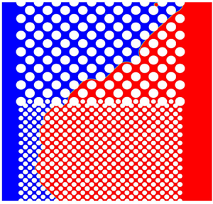
  $Ca_m$, the wetting fluid prefers to invade the low-permeability (high-permeability) zone and the breakthrough first occurs in the low-permeability (high-permeability) zone, consistent with the previous observations for the pore doublet. In all cases, very few drops of the non-wetting fluid are trapped as the residual phase in the imbibition process as the wetting fluid progresses. For figure 9(a–e) (
 $Ca_m=1.4574\text {--}72.8723$), we notice an oblique advancing pattern of the wetting fluid in both high- and low-permeability zones, but this phenomenon disappears when
  $Ca_m$ is increased up to
  $Ca_m=145.7446$ (figure 9f). This suggests that the oblique advancing of the wetting fluid arises from the non-trivial interfacial tension.

Figure 9. Fluid distributions in the dual-permeability pore network at breakthrough for (a)  $Ca_m=1.4574$, (b)
  $Ca_m=2.9149$, (c)
  $Ca_m=4.3723$, (d)
  $Ca_m=14.5745$, (e)
  $Ca_m=72.8723$ and (f)
  $Ca_m=145.7446$. The viscosity ratio of wetting to non-wetting fluids is fixed at 0.1. The non-wetting and wetting fluids are shown in red and blue, respectively.
To better understand the oblique advancing pattern, as an example, we plot the evolution of fluid distributions during the early imbibition at  $Ca_m=1.4574$, which is shown in figure 10. It is known that the dominant capillary pressure is larger in the smaller pores and throats according to the Young–Laplace equation, so the smallest pores and throats are filled first. For the present grain arrangement, let us take a close look at the interface between two vertically aligned solid grains A and B, as shown in figure 8(b). It is seen that a flat interface (represented by the blue solid line) with zero capillary pressure is able to touch the solid grain C, and thus the advancing meniscus of the wetting fluid always progresses towards the next column of grains through a triangle shape, as marked by the black triangles in figure 10. In addition, as shown in figure 10(f), as the wetting fluid invades the region marked by the black triangle, it cannot infiltrate in the direction highlighted by the dashed arrow due to the requirement of a positive pressure difference between the wetting and non-wetting fluids to overcome the capillary valve resistance (Xu et al. Reference Xu, Liu and Valocchi2017), but progress towards the direction highlighted by the solid arrow due to the merging with the neighbouring interface. As a result, the wetting fluid penetrates layer by layer along the direction indicated by the solid arrow, forming an oblique advancing pattern. A similar process occurs in the high-permeability zone, but in a direction perpendicular to the invading direction in the low-permeability zone. On the other hand, at the highest
  $Ca_m$ in figure 9(f), the aforementioned pore filling order is disrupted and no longer applicable, as here the viscous force dominates the imbibition behaviour.

Figure 10. Fluid distributions in the porous media geometry for  $Ca_m=1.4574$ and
  $\lambda =0.1$ at (a)
  $\hat t/\hat {t}_B=0.0145$, (b)
  $\hat t/\hat {t}_B=0.0217$, (c)
  $\hat t/\hat {t}_B=0.029$, (d)
  $\hat t/\hat {t}_B=0.0362$, (e)
  $\hat t/\hat {t}_B=0.0434$ and (f)
  $\hat t/\hat {t}_B=0.0507$. Each inset shows a close-up view of the region indicated by the black rectangular box in the lower left corner.
We then study the effect of viscosity ratio on the imbibition preference. A wide range of viscosity ratios, varying from  $\lambda =0.02$ to 50.0, is considered. For each viscosity ratio, at least three different values of
  $Ca_m$ are simulated, covering three typical patterns observed at breakthrough. The saturation data at breakthrough for various viscosity ratios and capillary numbers are listed in table 1, where
  $S_1$,
  $S_2$ and
  $S_w$ are the wetting fluid saturations in the low-permeability zone, the high-permeability zone and the entire pore network. Among all the cases considered, the maximum imbibition efficiency is obtained under the conditions of
  $\lambda =50$ and
  $Ca_m=0.08745$, where the wetting fluid saturations in both permeability zones are roughly the same (the corresponding values
  $S_1=0.8456$ and
  $S_2=0.8645$). In addition, for each viscosity ratio, the highest imbibition efficiency is always achieved when
  $S_1$ is closest to
  $S_2$. This implies that the critical capillary numbers
  $Ca_{m,c}$ represent the optimal condition to improve the imbibition efficiency.
Table 1. Saturations  $S_1$,
  $S_2$ and
  $S_w$ at breakthrough for various values of viscosity ratio (
 $\lambda$) and capillary number (
 $Ca_m$), where
  $S_{1}$ and
  $S_{2}$ are the wetting fluid saturations in the low- and high-permeability zone and
  $S_w$ is the wetting fluid saturation in the whole pore network.

To locate the values of  $Ca_{m,c}$ for different viscosity ratios, we extract the data regarding the imbibition preference from table 1 and plot them in the
  $\lambda$–
 $Ca_{m}$ diagram, as shown in figure 11. In this figure, the open symbols represent the cases where
  $S_1>S_2$, while the filled symbols represent the cases where
  $S_1 < S_2$. This means that for each value of
  $\lambda$, the critical capillary number
  $Ca_{m,c}$ lies between two nearest open and filled symbols. As such, the
  $Ca_{m,c}$ curve can be approximately obtained, which is represented by the green solid line. For the sake of comparison, figure 11 also plots the
  $Ca_{m,c}$ curve from the pore doublet model (represented by the blue dashed line and directly taken from figure 3). It is clear that the present
  $Ca_{m,c}$ curve overlaps well with the one from the pore doublet model. As shown in Appendix C and Appendix D, we also vary the permeability ratio (
 $k^2$) and the contact angle (
 $\theta$), and find that the results overall agree with the predictions from the pore doublet model. All of the results suggest that the simplified pore doublet model can provide insights into the physics of immiscible displacement in the more complex dual-permeability pore network.

Figure 11. The  $\lambda$–
 $Ca_m$ diagram showing preferential imbibition in a dual-permeability pore network. The open symbols represent the cases where
  $S_{1}>S_{2}$ at breakthrough (I), while the filled symbols represent the cases where
  $S_{1} < S_{2}$ at breakthrough (II). Two images of fluid distributions are shown as inserts depicting regions (I) and (II). The green solid line represents the
  $Ca_{m,c}$ curve, on which
  $S_1=S_2$ at breakthrough. The
  $Ca_{m,c}$ curve (represented by the blue dashed line) from the pore doublet model is also plotted for comparison.
Although the pore doublet model can predict the variation of  $Ca_{m,c}$ with
  $\lambda$ in a dual-permeability pore network, it is not clear whether the transient imbibition behaviour in the dual-permeability pore network can be correctly captured by the pore doublet model. In order to clarify this, we plot the time evolution of
  $S_1$ and
  $S_2$ (normalised by their maximum value at breakthrough) at three typical viscosity ratios in figure 12, where the semi-analytical solutions
  $\hat {L}_1$ and
  $\hat {L}_2$ (normalised by
  $\hat {L}$), obtained from (2.10) and (2.11) with the dimensionless numbers
  $Ca_m$ and
  $\lambda$ identical to those in the pore network, are also shown for comparison. For each viscosity ratio, the agreement between the LBM results and the semi-analytical solutions is generally better at higher
  $Ca_m$ where
  $S_1 < S_2$, but worse when
  $S_1>S_2$ where the interfacial tension is dominant. The larger discrepancy when
  $S_1>S_2$ (see figure 12a,c,e) is attributed to the fact that in the dual-permeability pore network, the interface varies and thus the capillary pressure varies when the meniscus moves from the throat to the pore body or from the pore body to the throat, while the capillary pressure remains constant in the pore doublet. We also increase the porosity to 0.62 in a similar pore network, and again observe a good agreement between the saturation evolution and the semi-analytical predictions, which is shown in Appendix E. In addition, we interestingly notice in figure 12(c) that after
  $\hat t/\hat {t}_B = 0.5$, the wetting fluid infiltrates into the high- and low-permeability zones alternately. Figure 13 shows the corresponding snapshots, from which it is seen that the wetting fluid invades only into the high-permeability zone in figure 13(a–c) and only into the low-permeability zone in figure 13(d–f).

Figure 12. The saturations in the low- and high-permeability regions (normalised by their maximum value at breakthrough) as a function of time in the dual-permeability pore network at  $\lambda =0.025$ for (a)
  $Ca_m=2.9149$ and (b)
  $Ca_m=5.8298$; at
  $\lambda =1$ for (c)
  $Ca_m=0.4372$ and (d)
  $Ca_m=7.2872$; at
  $\lambda =20.0$ for (e)
  $Ca_m=0.1457$ and (f)
  $Ca_m=0.2186$. The semi-analytical solutions from the pore doublet model at the same values of
  $\lambda$ and
  $Ca_m$ are also shown for the comparison.

Figure 13. Snapshots of the imbibition for  $Ca_m=0.4372$ and
  $\lambda =1$ at (a)
  $\hat t/\hat {t}_B=0.5106$, (b)
  $\hat t/\hat {t}_B=0.5532$, (c)
  $\hat t/\hat {t}_B=0.5957$, (d)
  $\hat t/\hat {t}_B=0.7234$, (e)
  $\hat t/\hat {t}_B=0.766$ and (f)
  $\hat t/\hat {t}_B=0.8085$. The snapshots from (a) to (f) correspond to the solid dots marked by A to F in figure 12(c).
4. Conclusions
We have studied the imbibition behaviour of two immiscible fluids in a dual-permeability pore network by a combination of pore-scale LBM simulation and mathematical modelling. First, we establish a mathematical model of the forced imbibition in a pore doublet, consisting of two branch channels with different widths, and find that the imbibition dynamics can be fully described by the viscosity ratio and the capillary number  $Ca_m$, which additionally incorporates the influence of channel width and length. By solving the mathematical model, a phase diagram of
  $\lambda$ versus
  $Ca_m$ is proposed to characterise the imbibition preference in the pore doublet. Then, the colour-gradient LBM is used to simulate the imbibition process in the pore doublet and its capability and accuracy are validated against the semi-analytical solutions of the mathematical model. Finally, the lattice Boltzmann simulations are used for the imbibition dynamics in a dual-permeability pore network. For each viscosity ratio, it is observed at breakthrough that the imbibition preferably occurs in the low-permeability zone at low values of
  $Ca_m$ but in the high-permeability zone at high values of
  $Ca_m$, which is attributed to the competition between capillary and viscous forces. When the capillary effects cannot be ignored, the wetting fluid is found to progress layer by layer in an oblique manner. In addition, for each viscosity ratio, there exists a critical capillary number
  $Ca_{m,c}$ at which the wetting fluid saturations are equal in both permeability zones, and
  $Ca_{m,c}$ represents the optimal condition to improve the imbibition efficiency. By comparing the phase diagram obtained for the dual-permeability pore network with that from the pore doublet model, we demonstrate for the first time that the pore doublet model can fairly well predict the variation of
  $Ca_{m,c}$ with the viscosity ratio in a dual-permeability pore network. Nevertheless, the pore doublet model cannot describe all features of the imbibition process in the dual-permeability pore network, especially when the imbibition preferably occurs in the low-permeability zone. The present study not only facilitates a fundamental understanding of the imbibition mechanism within dual-permeability porous media, but also provides operational guidelines to improve oil recovery in practice.
Funding
This work is supported by the National Natural Science Foundation of China (nos. 51876170, 12072257), the National Key Project (no. GJXM92579) and the Natural Science Basic Research Plan in Shaanxi Province of China (no. 2019JM-343). The computational resource is supported by the Center for Computational Science and Engineering of Southern University of Science and Technology.
Declaration of interests
The authors declare no conflict of interest.
Appendix A. Theoretical solution of critical capillary number in a pore doublet for  $\lambda =1$

When  $\lambda =1$, the explicit expressions for both
  $q_1$ and
  $q_2$ from (2.1), (2.2) and (2.3) can be obtained:
 \begin{gather} q_{1}=\frac{\left[\dfrac{3 \eta_n q L}{2 r_{2}^{3}}+\sigma \cos \theta\left(\dfrac{1}{r_{1}}-\dfrac{1}{r_{2}}\right)\right]}{1.5 \eta_n L\left(\dfrac{1}{r_{1}^{3}}+\dfrac{1}{r_{2}^{3}}\right)}, \end{gather}
 \begin{gather}q_{2}=\frac{\left[\dfrac{3 \eta_n q L}{2 r_{1}^{3}}-\sigma \cos \theta\left(\dfrac{1}{r_{1}}-\dfrac{1}{r_{2}}\right)\right]}{1.5 \eta_n L\left(\dfrac{1}{r_{1}^{3}}+\dfrac{1}{r_{2}^{3}}\right)}. \end{gather}
From  $q_2/q_1=r_2\cdot u_2/(r_1\cdot u_1)$, it is straightforward to write
 \begin{equation} \frac{u_2}{u_1}=\frac{k^2Ca_m+(1-k)k}{Ca_m - (1-k)k^2}. \end{equation}
In order to compare  $u_1$ and
  $u_2$, one can rewrite (A3) as
  ${u_2}/{u_1}\,{-}\,1\,{=}\,{((k^2-1)\cdot (Ca_m-k))}/ {(Ca_m + (k-1)k^2)}$. For
  $k>1$, it is easily obtained that when
  $Ca_m>k$,
  $u_2>u_1$ and thus the wetting fluid prefers to enter the large capillary (capillary 2 in figure 1); when
  $Ca_m < k$,
  $u_2 < u_1$ and thus the wetting fluid prefers to enter the small capillary (capillary 1); when
  $Ca_{m,c}=k$,
  $u_2=u_1$ and the breakthrough simultaneously occurs in both capillaries. This means that the critical capillary number
  $Ca_{m,c}=k$ for
  $\lambda =1$.
Appendix B. Lattice Boltzmann method for immiscible two-phase flow
Direct numerical simulation of the two-phase flow in two-dimensional pore spaces is performed using a state-of-the-art colour-gradient LBM (Xu et al. Reference Xu, Liu and Valocchi2017). In this model, the distribution functions  $f_{i}^{R}$ and
  $f_{i}^{B}$ are used to represent the red and blue fluids, where the subscript
  $i$ is the lattice velocity direction and ranges from 0 to 8 for the two-dimensional nine-velocity (D2Q9) lattice model used in this work. Function
  $f_{i}(\boldsymbol {x},t)$ is the total distribution function at position
  $\boldsymbol x$ and time
  $t$, and is defined as
  $f_{i}=f_{i}^{R}+f_{i}^{B}$. Conservation of mass for each fluid and total momentum conservation require
 \begin{equation} \rho^{k}=\sum_{i} f_{i}^{k}, \quad \rho \boldsymbol{u}=\sum_{i}f_{i}\boldsymbol{c}_{i},\quad k= R\text{ or }B, \end{equation}
where  $\rho =\rho ^{R}+\rho ^{B}$ is the total density with the superscripts ‘
 $R$’ and ‘
 $B$’ referring to the red and blue fluids, respectively, and
  $\boldsymbol u$ is the local fluid velocity. The lattice velocity
  $\boldsymbol c_i$ is defined as
  $\boldsymbol c_0=(0,0)$,
  $\boldsymbol c_{1,3}=(\pm c,0)$,
  $\boldsymbol c_{2,4}=(0,\pm c)$,
  $\boldsymbol c_{5,7}=(\pm c,\pm c)$ and
  $\boldsymbol c_{6,8}=(\mp c,\pm c)$, where
  $c=\delta _x/\delta _t$ is the lattice speed with
  $\delta _x$ being the lattice length and
  $\delta _t$ being the time step. The sound of speed is related to the lattice speed by
  $c_s=c/\sqrt {3}$. The evolution of
  $f_{i}^{R}$ and
  $f_{i}^{B}$ in time and space is described by
 \begin{equation} f_{i}^{k}(\boldsymbol{x}+\boldsymbol{c}_{i}\delta_t,t+\delta_t)=f_{i}^{k}(\boldsymbol{x},t) +{(\varOmega_{i}^{k})}^{(3)}[{(\varOmega_{i}^{k})}^{(1)}+{(\varOmega_{i}^{k})}^{(2)}], \end{equation}
where  ${(\varOmega _{i}^{k})}^{(1)}$ is the single-phase collision operator,
  ${(\varOmega _{i}^{k})}^{(2)}$ is the perturbation operator and
  ${(\varOmega _{i}^{k})}^{(3)}$ is the recolouring operator to guarantee the immiscibility of both fluids. Note that the single-phase collision and perturbation operators are to recover the Navier–Stokes equations for the fluid mixture, and thus can be implemented via the total distribution function
  $f_i$. Using the multiple relaxation time scheme (Ginzburg & d'Humieres Reference Ginzburg and d'Humieres2003), the single-phase collision operator reads as
 \begin{equation} (\varOmega_{i})^{(1)}={-}({\boldsymbol{\mathsf{M}}}^{{-}1}{\boldsymbol{\mathsf{SM}}})_{ij} (f_{j}-f_{j}^{eq}), \end{equation}
where  $f_{i}^{eq}$ is the equilibrium distribution function and is given by
 \begin{equation} f_{i}^{eq}(\rho, \boldsymbol{u})=\rho W_i\left[ 1+\frac{\boldsymbol{c}_i \cdot \boldsymbol{u}}{c_s^2}+\frac{(\boldsymbol{c}_i\cdot \boldsymbol{u})^2}{2c_s^4} -\frac{\boldsymbol{u}^2}{2c_s^2} \right]. \end{equation}
Herein,  $W_i$ is the weight factor with
  $W_{0}=4/9$,
  $W_{1-4}=1/9$ and
  $W_{5-8}=1/36$. The transformation matrix
  ${\boldsymbol{\mathsf{M}}}$ is given by (Lallemand & Luo Reference Lallemand and Luo2000)
 \begin{equation} {\boldsymbol{\mathsf{M}}} = \begin{bmatrix} 1 & 1 & 1 & 1 & 1 & 1 & 1 & 1 & 1\\ -4 & -1 & -1 & -1 & -1 & 2 & 2 & 2 & 2\\ 4 & -2 & -2 & -2 & -2 & 1 & 1 & 1 & 1\\ 0 & 1 & 0 & -1 & 0 & 1 & -1 & -1 & 1\\ 0 & -2 & 0 & 2 & 0 & 1 & -1 & -1 & 1\\ 0 & 0 & 1 & 0 & -1 & 1 & 1 & -1 & -1\\ 0 & 0 & -2 & 0 & 2 & 1 & 1 & -1 & -1\\ 0 & 1 & -1 & 1 & -1 & 0 & 0 & 0 & 0\\ 0 & 0 & 0 & 0 & 0 & 1 & -1 & 1 & -1 \end{bmatrix}. \end{equation}
 With the transformation matrix  ${\boldsymbol{\mathsf{M}}}$, the distribution function
  $f_i$ can be projected onto the moment space through
  $m_i = M_{ij}f_j$, and the resulting nine moments are
 \begin{equation} {\boldsymbol{\mathsf{m}}} = (\rho, e,\varepsilon,j_{x},q_{x},j_{y},q_{y},p_{xx},p_{xy})^{\textrm{T}}, \end{equation}
where  $e$ and
  $\varepsilon$ are related to the total energy and the energy square,
  $j_{x}$ and
  $j_{y}$ are the
  $x$ and
  $y$ components of the momentum,
  $q_{x}$ and
  $q_{y}$ are the components of the energy flux and
  $p_{xx}$ and
  $p_{xy}$ correspond to the diagonal and off-diagonal components of the viscous stress tensor. The values of the equilibrium moment are
  ${\boldsymbol{\mathsf{m}}}^{eq}=\rho (1,-2+3\boldsymbol {u}^2,1-3\boldsymbol {u}^2, u_x,-u_x, u^y,-u^y, u_x^2-u_y^2,u_x u_y)^{\textrm {T}}$, which are obtained by
  $m_i^{eq} = M_{ij}f_j^{eq}$. The diagonal relaxation matrix
  ${\boldsymbol{\mathsf{S}}}$ in (B3) is given as
  ${\boldsymbol{\mathsf{S}}}=\textrm {diag}(s_{\rho },s_{e},s_{\varepsilon },s_{j},s_{q},s_{j},s_{q},s_{p},s_{p} )$. Here
  $s_{\rho }$ and
  $s_{j}$ can take any values since they correspond to the conserved moments (density
  $\rho$ and momentum
  $\boldsymbol j$). Terms
  $s_{e}$ and
  $s_{p}$ are related to the bulk and shear viscosities, while
  $s_{\varepsilon }$ and
  $s_{q}$ are free parameters. To improve the numerical stability, we choose
  $s_{e}=s_{\varepsilon }=s_{p}=1/\tau$ and
  $s_{q}=8(2-s_{p})/(8-s_{p})$ (Pan, Luo & Miller Reference Pan, Luo and Miller2006) in our simulations, where the dimensionless relaxation time
  $\tau$ is related to the dynamic viscosity of the fluid mixture by
  $\eta =c_{s}^{2}\rho (\tau -0.5)\delta _t$. When both fluids have unequal viscosities, a harmonic mean is employed to determine the viscosity of the fluid mixture, i.e.
  $1/\eta =(1+\rho ^{N})/(2\eta ^{R})+(1-\rho ^{N})/(2\eta ^{B})$, where the phase field
  $\rho ^N$ is defined as
 \begin{equation} \rho^{N}(\boldsymbol{x},t)=\frac{\rho^{R}(\boldsymbol{x},t) -\rho^{B}(\boldsymbol{x},t)}{\rho^{R}(\boldsymbol{x},t)+\rho^{B}(\boldsymbol{x},t)}, \quad -1\leq \rho^N \leq 1. \end{equation}
 The perturbation operator that generates an interfacial force  $\boldsymbol {F}_{s}$ is given by
 \begin{equation} (\varOmega_{i})^{(2)}={\boldsymbol{\mathsf{M}}}^{{-}1}\left({\boldsymbol{\mathsf{I}}} -\frac{1}{2}{\boldsymbol{\mathsf{S}}}\right) \boldsymbol F, \end{equation}
with
 \begin{align} \boldsymbol{F}(\boldsymbol x,t)& = [0, 6(u_{x}F_{sx}+u_{y}F_{sy}), -6(u_{x}F_{sx}+u_{y}F_{sy}), \nonumber\\ &\quad F_{sx}, -F_{sx}, F_{sy}, -F_{sy}, 2(u_{x}F_{sx}-u_{y}F_{sy}), u_{x}F_{sy}+u_{y}F_{sx}]^{\textrm{T}}, \end{align}
where  ${\boldsymbol{\mathsf{I}}}$ is the second-order identity tensor and
  $F_{sx}$ and
  $F_{sy}$ are the components of the interfacial force
  $\boldsymbol {F}_{s}$. The interfacial tension between two fluids is modelled as a spatially varying body force
  $\boldsymbol F_s$ based on the continuum surface force concept (Brackbill, Kothe & Zemach Reference Brackbill, Kothe and Zemach1992), which is given by
 \begin{equation} \boldsymbol{F}_{s} =\tfrac{1}{2}\sigma K \boldsymbol{\nabla} \rho ^{N}, \end{equation}
where  $K$ is the local interface curvature related to the unit normal vector
  $\boldsymbol n$ by
 \begin{equation} K=n_{x}n_{y}\left(\frac{\partial}{\partial y}n_{x}+\frac{\partial}{\partial x}n_{y}\right)-n_{y}^2\frac{\partial}{\partial x}n_{x}-n_{x}^2\frac{\partial}{\partial y}n_{y}, \end{equation}
where  $n_x$ and
  $n_y$ are the
  $x$ and
  $y$ components of
  $\boldsymbol n$ defined by
  $\boldsymbol n =\boldsymbol {\nabla }\rho ^{N}/ | \boldsymbol {\nabla } \rho ^{N} |$. In the calculations of interface curvature and normal vector, the partial derivatives of a variable
  $\psi$ are evaluated by
 \begin{equation} \boldsymbol \nabla \psi (\boldsymbol{x},t)=\frac{1}{c_{s}^{2}}\sum_{i}W_{i}\psi(\boldsymbol{x}+\boldsymbol{c}_{i}\delta_{t},t)\boldsymbol{c}_{i}. \end{equation}
In the presence of interfacial force, the fluid velocity should be redefined as (Guo, Zheng & Shi Reference Guo, Zheng and Shi2002)
 \begin{equation} \rho \boldsymbol{u}=\sum_{i}f_{i}\boldsymbol{c}_{i}+\tfrac{1}{2}\boldsymbol{F}_{s}\delta_{t} \end{equation}
to correctly recover the Navier–Stokes equations. To minimise the mixing and segregate the red and blue fluids, the recolouring operator proposed by Latva-Kokko & Rothman (Reference Latva-Kokko and Rothman2005) is used:
 \begin{gather} (\varOmega_{i}^{R})^{(3)}(f_i^R)=\frac{\rho^{R}}{\rho }f_{i}^{*}+\beta \frac{\rho^{R}\rho^{B}}{\rho}W_i \cos(\varphi_{i}) |\boldsymbol{c}_{i}|, \end{gather}
 \begin{gather}(\varOmega_{i}^{B})^{(3)}(f_i^B)=\frac{\rho^{B}}{\rho }f_{i}^{*}-\beta \frac{\rho^{R}\rho^{B}}{\rho}W_i\cos(\varphi_{i})|\boldsymbol{c}_{i}|, \end{gather}
where  $f_{i}^{*}$ represents the total distribution function after the perturbation step. Here
  $\beta$ is a segregation parameter ranging from 0 to 1 and set to be 0.7 in order to maintain a narrow interface thickness and keep spurious velocities low (Halliday, Hollis & Care Reference Halliday, Hollis and Care2007). Angle
  $\varphi _{i}$ is the angle between
  $\boldsymbol {\nabla } \rho ^{N}$ and the lattice velocity
  $\boldsymbol {c}_{i}$.
On the solid surface, no-slip boundary condition is imposed using the halfway bounce-back scheme (Ladd Reference Ladd1994), and a wetting boundary condition is needed to obtain the desired contact angle  $\theta$. Here, the wetting boundary condition recently developed by Xu et al. (Reference Xu, Liu and Valocchi2017) is adopted, and its basic idea is to modify the orientation of the phase-field gradient at three-phase contact lines so as to match the desired contact angle. Because of its high accuracy and ability to deal with arbitrarily complex geometries, this wetting boundary condition has been used many times in pore-scale two-phase simulations (Gu, Liu & Zhang Reference Gu, Liu and Zhang2018; Xu & Liu Reference Xu and Liu2018; Gu et al. Reference Gu, Zhu, Zhang and Liu2019), and has been recently extended to the three-dimensional case (Akai, Bijeljic & Blunt Reference Akai, Bijeljic and Blunt2018). For the details of the wetting boundary condition, interested readers are referred to Xu et al. (Reference Xu, Liu and Valocchi2017).
Appendix C. The effect of permeability ratio
We now change the permeability ratio between the high- and low-permeability regions as  $k^2=9$ in order to further assess whether the pore doublet model is able to predict the imbibition preference in the dual-permeability pore network. The comparison between the imbibition preference in the dual-permeability pore network and the semi-analytical predictions from the pore doublet model is shown in figure 14, where only limited numerical tests are carried out for the sake of reducing computational burden. It is seen that for
  $k^2=9$, the
  $Ca_{m,c}$ curve obtained from the pore doublet model agrees with the imbibition preference in the dual-permeability pore network within acceptable accuracy.

Figure 14. Comparisons between the  $Ca_{m,c}$ curve (represented by the dashed line) from the pore doublet model and the imbibition preference (represented by the discrete symbols) in a dual-permeability pore network with permeability ratio
  $k^2=9$. The open symbols represent the cases where
  $S_{1}>S_{2}$ at breakthrough, while the filled symbols represent the cases where
  $S_{1} < S_{2}$ at breakthrough.
Appendix D. The effect of contact angle
We change the contact angle as  $\theta =15^\circ$ and
  $\theta =45^\circ$ in order to verify the prediction ability of the pore doublet model for imbibition preference in the dual-permeability pore network. The comparison between the imbibition preference in the dual-permeability pore network and the semi-analytical predictions from the pore doublet model is shown in figure 15, depicting results for
  $\theta =15^\circ$ and
  $\theta =45^\circ$. It is seen that the pore doublet model can reasonably predict the imbibition preference in the dual-permeability pore network for
  $\theta =45^\circ$ but its prediction accuracy is worse for
  $\theta =15^\circ$. This is because when the contact angle is very small, the capillary driving force which is relatively strong is a constant in the pore doublet model, while it is dynamically varying with the size of local pores and throats in the dual-permeability pore network.

Figure 15. Comparisons between the  $Ca_{m,c}$ curve (represented by the dashed lines) from the pore doublet model and the imbibition preference (represented by the discrete symbols) in a dual-permeability pore network for (a)
  $\theta =15^{\circ }$ and (b)
  $\theta =45^{\circ }$. The open symbols represent the cases where
  $S_{1}>S_{2}$ at breakthrough, while the filled symbols represent the cases where
  $S_{1} < S_{2}$ at breakthrough.
Appendix E. The effect of porosity
Consider a dual-permeability pore network with geometry similar to that in figure 8(a) but a different porosity of  $\epsilon =0.62$. We note that the permeability in the low-/high-permeability region increases compared with the geometry in figure 8(a) as the permeability in a staggered circular array can be calculated by
  $K=({\epsilon ^3(\epsilon -0.2146)}/{31(1-\epsilon )^{1.3}})d^2$ (
 $0.4345\leq \epsilon \leq 0.9372$) (Lee & Yang Reference Lee and Yang1997), where
  $d$ is the diameter of the solid cylinders. However, the permeability ratio between the high- and low-permeability regions is kept at
  $k^2=4$. We compare the saturation evolutions with the corresponding semi-analytical solutions from the pore doublet model in figure 16 and fairly good agreement is observed.

Figure 16. The saturations in the low- and high-permeability regions (normalised by their maximum value at breakthrough) as a function of time in the dual-permeability pore network at  $\lambda =0.1$ for (a)
  $Ca_m=2.3687$ and (b)
  $Ca_m=4.7374$; at
  $\lambda =1$ for (c)
  $Ca_m=1.1843$ and (d)
  $Ca_m=3.553$; at
  $\lambda =20$ for (e)
  $Ca_m=0.1777$ and (f)
  $Ca_m=0.2961$. The semi-analytical solutions from the pore doublet model at the same values of
  $\lambda$ and
  $Ca_m$ are also shown for comparison.


