


1. Introduction
The viscoelastic properties of dilute polymer solutions are central to several applications (Larson Reference Larson1999). When the pure solvent is turbulent the most remarkable effect of the addition of polymers is a significant reduction of the turbulent drag below that of the solvent (Procaccia, L'Vov & Benzi Reference Procaccia, L'Vov and Benzi2008; White & Mungal Reference White and Mungal2008; Benzi Reference Benzi2010; Graham Reference Graham2014). This phenomenon, also known as the Toms effect (Toms Reference Toms1949, Reference Toms1977), is commonly utilized to reduce the energy losses in pipelines and hence the costs associated with the transport of crude oil. However, in a turbulent flow, polymers are subject to mechanical degradation due to the fluctuating strain rate, which stretches polymers and thus causes their scission. Since turbulent drag reduction decreases with the molecular weight of the dissolved polymers (Virk Reference Virk1975), the efficacy of polymers as drag reducing agents diminishes in time, with a strong impact on both industrial applications and laboratory experiments (Paterson & Abernathy (Reference Paterson and Abernathy1970), Moussa, Tiu & Sridhar (Reference Moussa, Tiu and Sridhar1993), den Toonder et al. (Reference den Toonder, Draad, Kuiken and Nieuwstadt1995), Choi et al. (Reference Choi, Lim, Lai and Chan2002), Vanapalli, Islam & Solomon (Reference Vanapalli, Islam and Solomon2005), Vanapalli, Ceccio & Solomon (Reference Vanapalli, Ceccio and Solomon2006), Elbing et al. (Reference Elbing, Winkel, Solomon and Ceccio2009), Pereira & Soares (Reference Pereira and Soares2012), Owolabi, Dennis & Poole (Reference Owolabi, Dennis and Poole2017), see also the editorial of Poole (Reference Poole2020) and the review of Soares (Reference Soares2020)).
Analogous mechanical degradation and, by association, practical limitations are observed in experiments of homogeneous and isotropic turbulence with polymer additives (Crawford et al. Reference Crawford, Mordant, Xu and Bodenschatz2008). Indeed, even though in isotropic turbulence the mean strain rate is zero, on average line elements are stretched exponentially at a rate proportional to the inverse of the Kolmogorov dissipation time scale (Bec et al. Reference Bec, Biferale, Boffetta, Cencini, Lanotte, Musacchio and Toschi2006). At large Reynolds numbers, polymers therefore experience strong straining events that can highly distort them. This has been confirmed in experiments and numerical simulations, both directly by examination of the probability distribution of polymer extensions (Vaithianathan & Collins Reference Vaithianathan and Collins2003; Vincenzi et al. Reference Vincenzi, Jin, Bodenschatz and Collins2007, Reference Vincenzi, Perlekar, Biferale and Toschi2015; Jin & Collins Reference Jin and Collins2008; Watanabe & Gotoh Reference Watanabe and Gotoh2010) and indirectly through the observation of a strong polymer feedback on the flow (De Angelis et al. Reference De Angelis, Casciola, Benzi and Piva2005; Perlekar, Mitra & Pandit Reference Perlekar, Mitra and Pandit2006, Reference Perlekar, Mitra and Pandit2010; Crawford et al. Reference Crawford, Mordant, Xu and Bodenschatz2008; Ouellette, Xu & Bodenschatz Reference Ouellette, Xu and Bodenschatz2009; Xi, Bodenschatz & Xu Reference Xi, Bodenschatz and Xu2013; Watanabe & Gotoh Reference Watanabe and Gotoh2013a,Reference Watanabe and Gotohb, Reference Watanabe and Gotoh2014; de Chaumont Quitry & Ouellette Reference de Chaumont Quitry and Ouellette2016). Furthermore, experimental measurements of polymer scission in different channel flows, by Vanapalli et al. (Reference Vanapalli, Ceccio and Solomon2006), show that the majority of polymers reside, and therefore break up, in the bulk of the fluid, where the flow approximates isotropic turbulence, rendering the scission results independent of channel geometry.
Mechanical degradation has also been reported in the regime of elastic turbulence (Groisman & Steinberg Reference Groisman and Steinberg2004). Although the Reynolds number of the solution is low in this case, elastic instabilities generate a chaotic flow with highly fluctuating velocity gradients that stretch polymers up to their maximum length (Liu & Steinberg Reference Liu and Steinberg2014).
A detailed knowledge of the statistics of polymer scission in turbulent flows is thus important for the design of experiments and the performance of realistic simulations of both turbulent drag reduction and elastic turbulence. In laminar flows, considerable progress has been made in the modelling and simulation of polymer scission (e.g. Cascales & de la Torre Reference Cascales and de la Torre1991, Reference Cascales and de la Torre1992; Hsieh, Park & Larson Reference Hsieh, Park and Larson2005; Sim, Khomami & Sureshkumar Reference Sim, Khomami and Sureshkumar2007; Wu et al. Reference Wu, Li, Zheng and Xu2018). However, the knowledge gained from the study of laminar flows cannot be directly applied to turbulent flows because of the different properties of the strain rate, and consequently of the flow-induced polymer stretching, in the two types of flows. In an extensional velocity field, for instance, the probability distribution of polymer extensions is dominated by a peak that shifts towards larger extensions as the strain rate increases (Perkins, Smith & Chu Reference Perkins, Smith and Chu1997), and therefore scission is observed only for a sufficiently large strain rate. In contrast, for turbulent flows, the distribution of the extensions has a wide power-law core due to the intensely fluctuating strain rate (Balkovsky, Fouxon & Lebedev Reference Balkovsky, Fouxon and Lebedev2000; Watanabe & Gotoh Reference Watanabe and Gotoh2010; Liu & Steinberg Reference Liu and Steinberg2014). Hence the scission rate may be non-negligible even at moderate Reynolds numbers (proportional to the average magnitude of the fluctuating strain rate).
Unlike the fragmentation of liquid jets, sheets, or drops (Villermaux Reference Villermaux2007, Reference Villermaux2020), the modelling of flow-driven scission in turbulent polymer solutions is still in its infancy (Soares Reference Soares2020). The reason for this has to be sought in the difficulty of including the microscopic details of the scission process in constitutive models of polymer solutions. To our knowledge, the only continuum model that takes scission into account has been proposed by Pereira, Mompean & Soares (Reference Pereira, Mompean and Soares2018) and assumes that the maximum contour length is a spatiotemporal scalar field that decays due to scission while being transported by the fluid. Further development of continuum models requires an in depth understanding of the statistics of scission and the consequent reduction of the relaxation time – in addition to the decrease in the maximum contour length – of the polymer fragments.
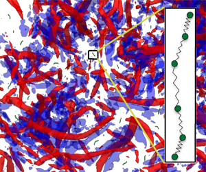
We therefore investigate the dynamics of polymers in a three-dimensional homogeneous and isotropic turbulent flow focusing on the scission statistics. A polymer is described as a bead-spring chain in a time-dependent, linear velocity field. This polymer model is known as the Rouse (Reference Rouse1953) model and represents one of the most common descriptions of a polymer molecule in a flow (in the case in which only two beads are considered, the Rouse model reduces to the elastic dumbbell model, see Bird et al. (Reference Bird, Curtiss, Armstrong and Hassager1977)). Even when the flow is turbulent, the assumption of a linear velocity field is justified, since the size of polymers is generally smaller than the Kolmogorov dissipation scale  $\eta _K$, below which viscosity strongly damps the spatial fluctuations of the velocity. We introduce scission into the Rouse model by assuming that the bead-spring chain breaks into two shorter chains as soon as the tension in one of the springs exceeds a critical threshold.
We begin by considering the statistics of the first scission. For passively transported polymers, for which the motion of the polymers does not modify the carrier velocity field, we derive qualitative analytical predictions by restricting ourselves to the Hookean dumbbell model and by using a decorrelated-in-time Gaussian stochastic velocity field (the approach is adapted from a study of droplet breakup conducted in Ray & Vincenzi (Reference Ray and Vincenzi2018)). The theoretical predictions are compared with Lagrangian direct numerical simulations (DNS) of the Rouse model in three-dimensional homogeneous isotropic turbulence. We then show that these results are qualitatively insensitive to the introduction of hydrodynamic interactions (HI) and excluded volume (EV) interactions among the beads of the polymer model. For active polymers, the statistics of the first scission is studied via hybrid Eulerian–Lagrangian simulations (Watanabe & Gotoh Reference Watanabe and Gotoh2013a,Reference Watanabe and Gotohb, Reference Watanabe and Gotoh2014), in which the feedback of (dumbbell-like) polymers onto the velocity field is taken into account. These simulations shed light on the transient nature of the dissipation-reduction effect, which owes its origin to polymer stretching and its demise to polymer scission. Finally, we analyse multiple scissions of passive polymers, via DNS in which a hierarchy of daughter polymers arise from successive breakups, each with their own statistics.
2. The Rouse chain
The Rouse model describes a polymer as a chain of  $\mathscr {N}$ inertialess beads connected to their nearest neighbours by elastic springs. We consider finitely extensible nonlinear elastic (FENE) springs with spring constant
  $H$ and maximum length
  $Q_m$. The fluid in which the chain is immersed is Newtonian and its motion is described by an incompressible velocity field
  $\boldsymbol {u}(\boldsymbol {x},t)$. The drag force of the fluid on each bead is given by Stokes law with drag coefficient
  $\zeta$; the collisions of the molecules of the fluid with a bead are described by Brownian motion. Finally, in the Rouse model, HI and EV interactions between different segments of the chain are disregarded. (These interactions do not affect the scission statistics qualitatively, as shown later in § 3.2.)
The motion of the chain is described in terms of the position of its centre of mass,  $\boldsymbol {X}_c$, and the separation vectors between the beads,
  $\boldsymbol {Q}_i$ (
 $i=1,\dots ,\mathscr {N}-1$). This set of coordinates evolves according to the equations (Bird et al. Reference Bird, Curtiss, Armstrong and Hassager1977; Öttinger Reference Öttinger1996)
 \begin{gather} \dot{\boldsymbol{X}}_c = \boldsymbol{u}(\boldsymbol{X}_c(t),t)+\dfrac{1}{\mathscr{N}}\sqrt{\frac{Q_{eq}^2}{6\tau}} \sum_{i=1}^{\mathscr{N}}\boldsymbol{\xi}_i(t),\end{gather}
 \begin{gather} \dot{\boldsymbol{Q}_i} = \boldsymbol{\kappa}(t)\boldsymbol{\cdot}\boldsymbol{Q}_i(t)-\dfrac{1}{4\tau} [2\,f_i\boldsymbol{Q}_i(t)-\,f_{i+1}\boldsymbol{Q}_{i+1}(t)-\,f_{i-1}\boldsymbol{Q}_{i-1}(t)] \nonumber\\ \quad+\sqrt{\dfrac{Q_{eq}^2}{6\tau}} [\boldsymbol{\xi}_{i+1}(t)-\boldsymbol{\xi}_i(t)],\quad i=1,\dots,\mathscr{N}-1, \end{gather}
where  $\kappa ^{\alpha \beta }(t)=\nabla ^\beta u^\alpha (\boldsymbol {X}_c(t),t)$ is the velocity gradient evaluated at the position of the centre of mass,
  $\tau =\zeta /4H$ is the characteristic time scale of the springs,
  $Q_{eq}=\sqrt {3k_BT/H}$ is their equilibrium root mean square (r.m.s.) extension (
 $k_B$ denotes the Boltzmann constant and
  $T$ is temperature), and
  $\boldsymbol {\xi }_i(t)$ (
 $i=1,\dots ,\mathscr {N}$) are independent, vectorial, white noises. The coefficients
 \begin{equation} f_i=\dfrac{1}{1-\vert\boldsymbol{Q}_i\vert^2/Q_m^2} \end{equation}
characterize the FENE interactions and ensure that the extension of each spring does not exceed its maximum length  $Q_m$. Obviously, in the equations for
  $\boldsymbol {Q}_1$ and
  $\boldsymbol {Q}_{\mathscr {N}-1}$ it is assumed that
  $\boldsymbol {Q}_0=\boldsymbol {Q}_{\mathscr {N}}=0$.
The end-to-end separation or extension vector of the polymer is defined as  $\boldsymbol {R}=\sum _{i=1}^{\mathscr {N}-1}\boldsymbol {Q}_i$. In a still fluid, the equilibrium r.m.s. value of
  $\vert \boldsymbol {R}\vert$ is
  $r_{eq}=Q_{eq}\sqrt {\mathscr {N}-1}$ (Bird et al. Reference Bird, Curtiss, Armstrong and Hassager1977).
We modify the Rouse model in order to account for the scission of the polymer when the tension in any of the springs exceeds a critical value. Since the relation between the tension and the extension of a spring can be easily inverted (Thiffeault Reference Thiffeault2003), we can, equivalently, assume that for each spring of the chain there exists a critical scission length  $\ell _{{sc}}$ such that the spring breaks if the length of the corresponding separation vector exceeds
  $\ell _{{sc}}$ (i.e. the chain breaks if
  $\vert \boldsymbol {Q}_i\vert \geqslant \ell _{{sc}}$ for any
  $1\leqslant i\leqslant \mathscr {N}-1$).
The scission process is non-stationary; the dynamics of the chain therefore depends on its initial configuration and, in particular, on its initial end-to-end separation  $r_0=\vert \boldsymbol {R}(0)\vert$. In the following we shall assume that
  $\ell _{{sc}}$ is much greater than
  $r_0/(\mathscr {N}-1)$ and that
  $r_0$ is equal to
  $r_{eq}$ or greater than it. (In principle, r 0 could also be taken smaller than
  $r_{eq}$, but we have checked that this case does not differ appreciably from the
  $r_0\simeq r_{eq}$ one.)
Finally, the size of the chain always remains smaller than  $\eta _{K}$, so that the velocity field at the scale of the chain can be considered as linear and the dynamics of the polymer is entirely determined by the velocity gradient at the location of the centre of mass, consistent with the Rouse model.
To summarize, the spatial scales that characterize the system are arranged as follows:  $r_{eq}\leqslant r_0\ll \ell _{{sc}}(\mathscr {N}-1) < Q_m(\mathscr {N}-1) < \eta _{K}$.
3. First-scission statistics
3.1. Passive polymers
3.1.1. Analytical predictions
Here we make some simplifying assumptions on both the polymer model and the carrier flow in order to derive analytical predictions for the statistics of polymer scission.
First of all, we only consider the statistics of the first scission. We then restrict ourselves to the  $\mathscr {N}=2$ case, also known as the dumbbell model (Bird et al. Reference Bird, Curtiss, Armstrong and Hassager1977; Öttinger Reference Öttinger1996), i.e. we focus on the slowest deformation mode of the polymer. Many results on single-polymer dynamics in random or turbulent flows have been obtained by using the dumbbell model (see Vincenzi et al. (Reference Vincenzi, Perlekar, Biferale and Toschi2015) and references therein) and the most common constitutive models of polymer solutions, namely the Oldroyd-B (Oldroyd Reference Oldroyd1950) and the FENE-P (Bird, Dotson & Johnson Reference Bird, Dotson and Johnson1980) models, are based on it. The legitimacy of this approach is supported by the numerical simulations in Jin & Collins (Reference Jin and Collins2008) and Watanabe & Gotoh (Reference Watanabe and Gotoh2010), where it is shown that, in isotropic turbulence and in the absence of scission, the statistics of the end-to-end separation of a dumbbell and that of an
  $\mathscr {N}=20$ chain coincide (provided, of course, that a proper mapping between the parameters of the two systems is applied). Finally, we replace the nonlinear spring with a Hookean one (
 $f_i=1$); this is because the nonlinearity of the elastic force enters into play only at extensions close to the scission length, and we shall see from our simulations in § 3.1.2 that it does not affect the qualitative properties of the scission process. For
  $\mathscr {N}=2$, (2.1) reduce to
 \begin{gather} \dot{\boldsymbol{X}}_c = \boldsymbol{u}(\boldsymbol{X}_c(t),t)+\dfrac{1}{2}\sqrt{\frac{r_{eq}^2}{3\tau}} \,\boldsymbol{\zeta}_1(t), \end{gather}
 \begin{gather}\dot{\boldsymbol{R}} = \boldsymbol{\kappa}(t)\boldsymbol{\cdot}\boldsymbol{R}(t)-\dfrac{\boldsymbol{R}(t)}{2\tau} +\sqrt{\dfrac{r_{eq}^2}{3\tau}}\, \boldsymbol{\zeta}_2(t), \end{gather}
where  $\boldsymbol {\zeta }_1(t)$ and
  $\boldsymbol {\zeta }_2(t)$ are (non-independent) vectorial white noises.
We model the flow via the smooth (also known as Batchelor) regime of the Kraichnan (Reference Kraichnan1968) model. This model has been widely employed in the study of turbulent transport (Falkovich, Gawȩdzki & Vergassola Reference Falkovich, Gawȩdzki and Vergassola2001) and has yielded several theoretical results on the coil-stretch transition in random or turbulent flows (see Plan, Ali & Vincenzi (Reference Plan, Ali and Vincenzi2016) and references therein). The velocity is a divergenceless and spatially smooth Gaussian vector field. It is statistically stationary in time and homogeneous, isotropic, and parity invariant in space; it has zero mean and zero correlation time. Under these assumptions,  $\boldsymbol {\kappa }(t)$ is a tensorial white noise with two-time correlation (Falkovich et al. Reference Falkovich, Gawȩdzki and Vergassola2001)
 \begin{equation} \langle \kappa^{ij}(t)\kappa^{mn}(t')\rangle= \mathscr{K}^{ijmn}\delta(t-t'), \end{equation}
where
 \begin{equation} \mathscr{K}^{ijmn}=\frac{\lambda}{3} [4\delta^{im}\delta^{jn}-\delta^{ij} \delta^{mn}-\delta^{in}\delta^{jm}] \end{equation}
and  $\lambda$ is the maximum Lyapunov exponent of the flow. Obviously, the assumption of temporal decorrelation is a strong approximation, since an isotropic turbulent flow has Kubo number
  $\mathit {Ku}=\lambda t_{{corr}}\approx 0.6$, where
  $t_{{corr}}$ is the correlation time of the flow (Girimaji & Pope Reference Girimaji and Pope1990; Bec et al. Reference Bec, Biferale, Boffetta, Cencini, Lanotte, Musacchio and Toschi2006; Watanabe & Gotoh Reference Watanabe and Gotoh2010). However, it was shown in Musacchio & Vincenzi (Reference Musacchio and Vincenzi2011) that, for a stochastic flow with comparable
  $\mathit {Ku}$, the statistics of polymer extension is captured qualitatively by a time decorrelated velocity field.
The Weissenberg number  $\mathit {Wi}=\lambda \tau$ determines to what extent polymers are stretched by the flow. In particular, the coil-stretch transition occurs when
  $\mathit {Wi}$ exceeds the critical value
  $\mathit {Wi}_{cr}=1/2$ ( (Lumley Reference Lumley1972; Balkovsky et al. Reference Balkovsky, Fouxon and Lebedev2000) – note that our definition of
  $\tau$ and hence that of
  $\mathit {Wi}$ differ from that of Balkovsky et al. (Reference Balkovsky, Fouxon and Lebedev2000) by a factor of 2).
As the velocity field is homogeneous and isotropic in space, the statistics of  $R=\vert \boldsymbol {R}\vert$ is independent of the position of the centre of mass and of the direction of
  $\boldsymbol {R}$. To study polymer scission, it is therefore sufficient to focus on the probability density function (p.d.f.) of
  $R$, which will be denoted as
  $P(R,t)$. When
  $\boldsymbol {\kappa }(t)$ has the properties described above,
  $P(R,t)$ satisfies the Fokker–Planck equation (Chertkov Reference Chertkov2000; Celani, Musacchio & Vincenzi Reference Celani, Musacchio and Vincenzi2005)
 \begin{equation} \partial_{t'} P=\mathbb{L} P,\quad \mathbb{L} P=- \partial_R (D_1 P)+\partial_R^2(D_2 P), \end{equation}
with rescaled time  $t'=t/2\tau$ and coefficients
 \begin{equation} D_1 = \left(\frac{8}{3}\mathit{Wi}-1\right)R+\dfrac{2r_{eq}^2}{3R}, \quad D_2 = \frac{2\mathit{Wi}}{3}R^2+\frac{r_{eq}^2}{3} \end{equation}
(once again our definition of  $\mathit {Wi}$ differs from that used in Chertkov (Reference Chertkov2000) and Celani et al. (Reference Celani, Musacchio and Vincenzi2005) by a factor of 2). The appropriate boundary conditions are reflecting at
  $R=0$ and absorbing at
  $R=\ell _{{sc}}$, i.e.
 \begin{equation} D_1 P-\partial_R(D_2 P)=0 \quad \text{at $R=0$} \quad \text{and} \quad P(\ell_{{sc}},t)=0 \end{equation}
for all  $t$. The former condition ensures that the extension of the polymer stays positive, while the latter describes scission at
  $R=\ell _{{sc}}$. The analysis of (3.4a,b) to (3.6) closely follows that in Ray & Vincenzi (Reference Ray and Vincenzi2018) for the breakup of sub-Kolmogorov droplets in isotropic turbulence. (The results presented here are deduced directly from those in § 3 of Ray & Vincenzi (Reference Ray and Vincenzi2018) by setting
  $\mathit {Ca}=\mathit {Wi}$,
  $\mu =1$,
  $r_{{eq}}^2= Q_{eq}^2/3$, and
  $f_1(\mu )=\,f_2(\mu )=\gamma (\mu )=1$.) We therefore skip the details of the derivations and directly present the predictions of scission statistics.
The number of unbroken polymers that survive at time  $t$,
$t$,  $N_p(t)$, is related to
  $P(R,t)$ as follows:
 \begin{equation} N_p(t)/N_p(0)=\int_0^{\ell_{{sc}}} P(R,t)\,\mathrm{d}R. \end{equation}
At times  $t\gg \tau$,
  $N_p(t)$ therefore decays exponentially as
 \begin{equation} N_p(t)\sim N_p(0)\,\textrm{e}^{-t/T_d}, \end{equation}
where the decay time  $T_d$ is the reciprocal of the lowest eigenvalue of the operator
  $\mathbb {L}$ with boundary conditions (3.6). The eigenfunctions of
  $\mathbb {L}$ are hypergeometric functions with parameters depending on
  $r_{eq}$,
  $r_0$,
  $\mathit {Wi}$ and form a discrete set selected by the boundary condition at
  $R=\ell _{{sc}}$. A calculation of the lowest eigenvalue shows that
  $T_d$ depends weakly on
  $\mathit {Wi}$ for small
  $\mathit {Wi}$, decreases rapidly as
  $\mathit {Wi}$ exceeds
  $\mathit {Wi}_{cr}$, and saturates at large
  $\mathit {Wi}$.
As we shall see below, the p.d.f. of  $R$ integrated over time,
 \begin{equation} \hat{P}(R)=\int_0^\infty P(R,t)\,\mathrm{d}t, \end{equation}
allows us to estimate the mean lifetime of a polymer before its first scission. If the initial distribution of polymer sizes is ‘monodisperse’, i.e.  $P(R,0)=\delta (R-r_0)$, then
  $\hat {P}(R)$ takes the form
 \begin{equation} \hat{P}(R)\propto \begin{cases} \textrm{e}^{-\varPhi(R)}[\phi(\ell_{{sc}})-\phi(r_0)] & \text{if $0\leqslant R\leqslant r_0$}, \\ \textrm{e}^{-\varPhi(R)}[\phi(\ell_{{sc}})-\phi(R)] & \text{if $r_0< R\leqslant\ell_{{sc}}$} \end{cases} \end{equation}
with
 \begin{equation} \varPhi(R)=\ln D_2(R)-\int^R \dfrac{D_1(\zeta)}{D_2(\zeta)}\,\mathrm{d}\zeta, \quad \phi(R)=\int^R \dfrac{\textrm{e}^\varPhi(\zeta)}{D_2(\zeta)}\,\mathrm{d}\zeta \end{equation}
and hence
 \begin{equation} \hat{P}(R)\sim \begin{cases} r_{eq}^{-2}r_0^ {-1}R^2 & \text{if $0\leqslant R\ll r_{eq}$,}\\ \vert r_0^\alpha-\ell_{{sc}}^\alpha\vert R^{-1-\alpha} & \text{if $r_{eq}\ll R\ll r_0$,}\\ \ell_{{sc}}^\beta R^{-1-\beta} & \text{if $r_0\ll R\ll\ell_{{sc}}$}, \end{cases} \end{equation}
where  $\alpha =3(\mathit {Wi}^{-1}-2)/2$ and
 \begin{equation} \beta = \begin{cases} \alpha & \text{if $\mathit{Wi}<\mathit{Wi}_{cr}$,}\\ 0 & \text{if $\mathit{Wi}>\mathit{Wi}_{cr}$}. \end{cases} \end{equation}
Therefore, above the coil-stretch transition, the right-hand tail of  $\hat {P}(R)$ saturates to the power-law
  $R^{-1}$. An analogous behaviour was found previously for the size distribution of sub-Kolmogorov droplets in isotropic turbulence (Biferale, Meneveau & Verzicco Reference Biferale, Meneveau and Verzicco2014; Ray & Vincenzi Reference Ray and Vincenzi2018). Also note that the exponent
  $\alpha$ coincides with the one obtained by Balkovsky et al. (Reference Balkovsky, Fouxon and Lebedev2000) for the p.d.f. of intermediate extensions in the absence of scission.
If the initial distribution of polymer sizes is broad but nonetheless admits a maximum size  $r_0$, then the left (
 $R\ll r_{eq}$) and right (
 $r_0\ll R\ll \ell _{{sc}}$) power-law tails continue to exist, but
  $\hat {P}(R)$ no longer behaves as a power-law for extensions
  $r_{eq}\ll R\ll r_0$.
The mean time  $\langle T _{{sc}}\rangle$ it takes for a polymer to undergo its first scission can be deduced from the behaviour of
  $\hat {P}(R)$ via the relation
 \begin{equation} \langle T_{{sc}}\rangle=\int_0^{\ell_{{sc}}}\hat{P}(R)\,\mathrm{d}R. \end{equation}
Equation (3.12) then yields two different behaviours below and above the coil-stretch transition
 \begin{equation} \lambda\langle T_{{sc}}\rangle\sim \begin{cases} (\ell_{{sc}}/r_0)^\beta & \text{if $\mathit{Wi}<\mathit{Wi}_{cr}$},\\ \ln (\ell_{{sc}}/r_0) & \text{if $\mathit{Wi}>\mathit{Wi}_{cr}$}. \end{cases} \end{equation}
3.1.2. DNS
In this section, we present numerical simulations of the Rouse model (2.1) in homogeneous and isotropic turbulence and compare them with the analytical predictions of § 3.1.1. The velocity field  $\boldsymbol {u}(\boldsymbol {x},t)$ is the solution of the incompressible Navier–Stokes equations,
 \begin{equation} \partial_t \boldsymbol{u}+\boldsymbol{u}\boldsymbol{\cdot}\boldsymbol{\nabla}\boldsymbol{u}=- \boldsymbol{\nabla} p+\nu_f\Delta\boldsymbol{u}+\boldsymbol{F}, \quad \boldsymbol{\nabla}\boldsymbol{\cdot}\boldsymbol{u}=0, \end{equation}
over the periodic cube  $[0,2{\rm \pi} ]^3$. Here
  $p$ is pressure,
  $\nu _f$ is the kinematic viscosity and
  $\boldsymbol {F}(\boldsymbol {x},t)$ is a body force that maintains a constant kinetic energy input
  $\epsilon _{in}$. The numerical integration uses a standard, fully dealiased pseudo-spectral method with
  $512^3$ collocation points and, for the time evolution, a second-order slaved Adams–Bashforth scheme with time step
  $\textrm {d}t=4\times 10^{-4}$. The values of
  $\nu _f$ and
  $\epsilon _{in}$ are such that the Taylor-microscale Reynolds number is
  $\mathit {Re}_\lambda =111$. The Lyapunov exponent of the flow is
  $\lambda =0.15\tau _\eta ^{-1}$, where
  $\tau _\eta$ denotes the Kolmogorov time scale, consistent with the value found earlier in Bec et al. (Reference Bec, Biferale, Boffetta, Cencini, Lanotte, Musacchio and Toschi2006) and Watanabe & Gotoh (Reference Watanabe and Gotoh2010).
The position of the centre of mass of the polymer is obtained by integrating (2.1a) via a second-order Adam–Bashforth method with the same  $\textrm {d}t$ as for the Navier–Stokes equations. The noise term in (2.1a) is disregarded, because it has a negligible effect when
  $\boldsymbol {u}(\boldsymbol {x},t)$ is turbulent. Moreover, its amplitude is smaller than that of the noise terms in the equations for the separation vectors by a factor of
  $\mathscr {N}$. As
  $\boldsymbol {u}(\boldsymbol {x},t)$ is only known over a discrete grid, the integration of (2.1a) requires interpolation to reconstruct the velocity field at
  $\boldsymbol {X}_c(t)$ – a trilinear scheme is used for this purpose. The same approach allows the calculation of the velocity gradient along the trajectory of the centre of mass,
  $\boldsymbol {\kappa }(t)$, and hence the integration of (2.1b) by means of the Euler–Maruyama method with time step
  $\textrm {d}t$. Since in this section we focus on the statistics of the first scission, a chain is removed from the simulation as soon as it breaks according to the criterion discussed above. The time origin for (2.1b) (
 $t=0$) is taken in the statistically steady state of the carrier turbulent flow, so that the temporal dynamics of polymers is not influenced by the initial transient evolution of
  $\boldsymbol {u}(\boldsymbol {x},t)$. Note that, in the present context, it is not necessary to use integration schemes specifically designed to prevent the extension of the links from exceeding
  $Q_m$, since the links, by construction, break well before their extension approaches
  $Q_m$.
In our simulations, we consider  $N_p(0)=9\times 10^5$ polymers, whose positions at time
  $t=0$ are uniformly distributed in space. Since the statistics of polymer extension depends on the initial size of polymers but not on their orientation, for simplicity the initial condition for the separation vectors is taken to be
  $\boldsymbol {Q}_i(0)=Q_0 (1,1,1)/\sqrt {3}$ with
  $Q_0>0$ for all polymers, i.e. the polymers are in a straight configuration and
  $P(R,0)=\delta (R-r_0)$ with
  $r_0=(\mathscr {N}-1)Q_0$.
In order to compare chains with different numbers of beads, an appropriate mapping of the chain parameters is needed. We use the mapping proposed by Jin & Collins (Reference Jin and Collins2008) and also used by Watanabe & Gotoh (Reference Watanabe and Gotoh2010). If the parameters of the individual links of an  $\mathscr {N}$-bead chain are
  $\tau$,
  $Q_{eq}$,
  $Q_m$,
  $\ell _{{sc}}$, then the statistics of the end-to-end separation of the chain is equivalent to that of a dumbbell with the following parameters:
 \begin{align} \tau^{D}=\frac{\mathscr{N}(\mathscr{N}+1)\tau}{6}, \quad Q_{eq}^D=Q_{eq}, \quad Q_m^{D}=Q_m{\sqrt{\mathscr{N}-1}}, \quad \ell_{{sc}}^{D}=\ell_{{sc}}{\sqrt{\mathscr{N}-1}}, \end{align}
where the last relation is introduced for compatibility with the expression of  $Q_m^D$. This mapping allows us to compare chains with different numbers of beads by using the dumbbell model as a reference.
Following Watanabe & Gotoh (Reference Watanabe and Gotoh2010), we define the Weissenberg number for a Rouse chain as  $\mathit {Wi}=\lambda \tau ^{D}$. In our simulations,
  $0.4\leqslant \mathit {Wi} \leqslant 8$. (Note that small-
 $\mathit {Wi}$ simulations are computationally more demanding, because the calculation of quantities like
  $\hat {P}(R)$ and
  $\langle T _{{sc}}\rangle$ requires that the time evolution is long enough for all polymers to break, and the time at which the scission process is complete becomes longer and longer as
  $\mathit {Wi}$ decreases.)
As for the choice of the other parameters, we take  $r_{eq}=1$,
  $Q_m^{D}=\sqrt {3000}$ (also following Jin & Collins (Reference Jin and Collins2008) and Watanabe & Gotoh (Reference Watanabe and Gotoh2010)), and, unless otherwise specified,
  $r_0=r_{eq}$. In addition, it is assumed that a spring breaks as soon as its extension exceeds
  $\ell _{{sc}}=0.8Q_m$. The number of beads is set to
  $\mathscr {N}=10$. We have also performed simulations with different sets of parameters, which support the generality of the results presented below.
It is worth mentioning that the above parameters are compatible with those of the experiment of Crawford et al. (Reference Crawford, Mordant, Xu and Bodenschatz2008), which investigates bulk turbulence in a water solution of polyacrylamide (known as PAM) with molecular weight  $M_w=18\times 10^6$, maximum extension
  $L=77\ \mathrm {\mu } \textrm {m}$ and relaxation time
  $\tau _p=43\ \textrm {ms}$. Mechanical degradation is observed at
  $R_\lambda =485$. For this value of
  $R_\lambda$, the Kolmogorov time scale is reported to be
  $\tau _\eta =2.63\ \textrm {ms}$, and hence the Weissenberg number based on the Lyapunov exponent can be estimated as
  $\mathit {Wi}\approx 2.5$.
Figure 1(a) shows the temporal evolution of the fraction of unbroken polymers. The decay is exponential with a time scale  $T_d$ that decreases rapidly as
  $\mathit {Wi}$ exceeds its critical value (figure 1b), in agreement with the predictions of § 3.1.1. We shall see in § 3.3 that, for a dumbbell, it is possible to write an explicit expression for
  $T_d$ as a function of
  $\mathit {Wi}$.

Figure 1. Passive polymers: (a) exponential decay of the fraction of unbroken polymers for different values of  $\mathit {Wi}$; (b) decay time of the fraction of unbroken polymers rescaled by the Kolmogorov time
  $\tau _\eta$ as a function of
  $\mathit {Wi}/\mathit {Wi}_{cr}$.
The time-integrated p.d.f. of the end-to-end extension of unbroken polymers is shown in figure 2(a) for an initial polymer size  $r_0=r_{eq}$ and different values of
  $\mathit {Wi}$. The p.d.f. displays a power-law behaviour for both
  $R\ll r_{eq}$ and
  $r_0=r_{eq}\ll R\ll \ell _{{sc}}(\mathscr {N}-1)$. The left-hand tail is proportional to
  $R^2$, because the small separations are dominated by thermal fluctuations. The right-hand tail rises as a function of
  $\mathit {Wi}$, until the power-law saturates to
  $R^{-1}$ for
  $\mathit {Wi}>\mathit {Wi}_{cr}$. A third power-law emerges for intermediate extensions if
  $r_0>r_{eq}$ (figure 2b). In this case, the exponent
  $-1-\alpha$ changes from negative to positive as
  $\mathit {Wi}$ increases and saturates to
  $2$ at large
  $\mathit {Wi}$. To appreciate the coexistence of these three power-laws more clearly, in figure 3a we also consider
  $\hat {P}(R)$ for a much larger value of
  $Q_m^D$ and a larger separation between
  $r_{eq}$,
  $r_0$ and
  $(\mathscr {N}-1)\ell _{{sc}}$. All these results confirm the predictions reported in § 3.1.1.

Figure 2. Passive polymers: (a) time-integrated p.d.f. of the end-to-end extension of unbroken polymers for  $r_0=r_{eq}$ and for different values of
  $\mathit {Wi}$. The inset shows the value of
  $\beta$, which determines the exponent of the right-hand tail of the p.d.f. (i.e.
  $\hat {P}(R)\propto R^{-1-\beta }$ for
  $r_0\ll R\ll \ell _{{sc}}$), as a function of
  $\mathit {Wi}/\mathit {Wi}_{cr}$; (b) time-integrated p.d.f. of the end-to-end extension of unbroken polymers for
  $r_0=40r_{eq}$ and for different values of
  $\mathit {Wi}$. The inset shows the value of
  $\alpha$, which determines the power-law behaviour of the p.d.f. for intermediate extensions (i.e.
  $\hat {P}(R)\propto R^{-1-\alpha }$ for
  $r_{eq}\ll R\ll r_0$), as a function of
  $\mathit {Wi}/\mathit {Wi}_{cr}$. In both panels (a) and (b), the p.d.f.s are normalized to unity for the sake of comparison.

Figure 3. Passive polymers: (a) time-integrated p.d.f. of the end-to-end extension of unbroken polymers for  $Q^D_m=10^4$,
  $r_{eq}=1$,
  $r_0=10^2$ and different values of
  $\mathit {Wi}$; (b) time-integrated p.d.f. of the end-to-end extension of unbroken polymers for
  $Q^{D}_m=10^4$,
  $r_{eq}=1$,
  $r_0=5\times 10^2$,
  $\mathit {Wi}=1$, and an initial size distribution that is either monodisperse (dotted magenta line) or uniform (between
  $r_{eq}$ and
  $r_0$; solid grey line). In both panels, the p.d.f.s are normalized to unity for the sake of comparison.
The p.d.f.s presented so far correspond to a ‘monodisperse’ initial state  $P(R)=\delta (R-r_0)$ in which all polymers have the same end-to-end distance. However, as mentioned in § 3.1.1, the behaviour of
  $\hat {P}(R)$ for intermediate extensions is expected to change if the initial distribution of polymer extensions is broad. To confirm this prediction, we have considered an initial state in which the end-to-end distance of polymers is distributed uniformly between
  $r_{eq}$ and a maximum initial extension
  $r_0>r_{eq}$. The time-integrated p.d.f.s given in figure 3(b) show that only the left- and right-hand power-law tails persist in this case, while
  $\hat {P}(R)$ does not behave as a power-law for intermediate extensions.
We now turn to the statistics of the lifetime  $T_{{sc}}$ of a polymer. The DNS suggest that the p.d.f. of
  $T_{{sc}}$ has an exponential tail with a time scale
  $\gamma ^{-1}$ that, beyond
  $\mathit {Wi}_{cr}$, decreases rapidly as a function of
  $\mathit {Wi}$ (figure 4a). For all values of the Weissenberg number,
  $\gamma ^{-1}$ is approximately the same as the decay time
  $T_d$ of the fraction of unbroken polymers owing to the exponential decay of the latter at long times (see § 3.1.1). However,
  $\gamma ^{-1}$ differs from
  $\langle T_{ sc}\rangle$, because the exponential behaviour of the p.d.f. of
  $T_{{sc}}$ sets in only at relatively large values of
  $T_{{sc}}$. For a fixed
  $\mathit {Wi}$, the mean lifetime
  $\langle T_{sc}\rangle$ behaves as a power of
  $\ell _{{sc}}/Q_0$ below the coil-stretch transition and as the logarithm of
  $\ell _{{sc}}/Q_0$ beyond that (see figures 4b and 4c) – we remind the reader that
  $Q_0$ is the initial length of any link of the chain. Small deviations are only observed for
  $\ell _{{sc}}\gg Q_0$. Moreover, we have checked that, for
  $\mathit {Wi}<\mathit {Wi}_{cr}$, the exponent
  $\beta$ that gives the dependence of
  $\langle T _{{sc}}\rangle$ on
  $\ell _{{sc}}/Q_0$ is the same as the exponent that describes the right-hand tail of
  $\hat {P}(R)$, i.e.
  $\hat {P}(R)\propto R^{-1-\beta }$ for
  $r_0\ll R\ll (\mathscr {N}-1) \ell _{{sc}}$, in agreement with (3.15). Thus, the statistics of
  $T_{{sc}}$ in a turbulent flow is correctly described by the predictions of § 3.1.1.

Figure 4. Passive polymers: (a) p.d.f. of the lifetime of a polymer for different values of  $\mathit {Wi}$. The inset compares the decay time of the fraction of unbroken polymers, the mean lifetime of a polymer and the time scale
  $\gamma ^{-1}$ in the exponential tail of the p.d.f. (
 $P(T_{sc})\sim \textrm {e}^{-\gamma T_{sc}}$ for
  $T_{sc}/\tau _\eta \gg 1$) as a function of
  $\mathit {Wi}/\mathit {Wi}_{cr}$; (b) mean lifetime as a function of
  $\ell _{{sc}}/Q_0$ below the coil-stretch transition. Here
  $T_{sc}'$ is a fitting parameter for the dashed lines. The data for
  $\mathit {Wi}=0.4$ (respectively,
  $\mathit {Wi}=0.45$) are multiplied by a factor of
  $10^2$ (respectively, 10) in order to make the three lines more easily distinguishable; (c) the same as in panel (b) above the coil-stretch transition.
We also note that the exponential tail of the distribution of  $T_{sc}$ originates from the fact that scission is caused by the cumulative action of the fluctuating strain rate. This is in contrast to the fragmentation of sub-Kolmogorov inextensible fibres, for which the internal tension depends on the instantaneous velocity gradient projected along the fibre. The p.d.f. of the scission time for fibres, therefore, reflects the intermittent statistics of the velocity gradient and is strongly non-exponential (Allende, Henry & Bec Reference Allende, Henry and Bec2020).
Figure 5 presents further results on the statistics of the scission process. As previously observed in experiments (Horn & Merrill Reference Horn and Merrill1984), scission preferentially happens at the midpoint of the polymer. However, the probability of scission happening at the middle link decreases with  $\mathit {Wi}$. The reason for this is that, for small
  $\mathit {Wi}$, the chain is most of the time in a coiled state and scission occurs because of a sequence of very strong fluctuations of
  $\boldsymbol {\nabla }\boldsymbol {u}$, whereas for large
  $\mathit {Wi}$ all links are consistently stretched near to the scission length. The insets of figure 5 show that the probability of more than one link breaking simultaneously is generally very small.

Figure 5. Passive polymers: probability of polymer scission occurring at the  $j_{sc}$-th link for different values of
  $\mathit {Wi}$. The insets shows the probability of
  $n_L$ links breaking simultaneously.
Finally, it was mentioned in § 3.1.1 that, in the absence of scission, the dumbbell model ( $\mathscr {N}=2$) captures the statistics of the end-to-end extension of a full chain remarkably well, provided the mapping in (3.17a–d) is applied (see Watanabe & Gotoh Reference Watanabe and Gotoh2010). We have performed an analogous comparison in the presence of scission. The time-integrated p.d.f.s in figure 6(a) show that, after the parameters of the chain are suitably rescaled, the time-independent statistics of the end-to-end distance is independent of
  $\mathscr {N}$, except for small deviations close to the maximum extension. Indeed, for a dumbbell, scission is defined in terms of the end-to-end separation, whereas chains with larger
  $\mathscr {N}$ break before all the links can stretch up to
  $\ell _{{sc}}$. These small differences, however, have a significant impact on time-dependent quantities, such as the fraction of unbroken polymers: small-
 $\mathscr {N}$ chains capture the temporal decay qualitatively, but underestimate the scission rate (see figure 6b). The results also suggest that the discrepancies between chains with
  $\mathscr {N}-1$ and
  $\mathscr {N}$ beads diminish as
  $\mathscr {N}$ increases (figure 6b) as well as when
  $\mathit {Wi}$ increases (not shown). We conclude that it is important to consider the dynamics of a full bead-spring chain in order to accurately describe the scission process and achieve quantitative agreement between experiments and models of polymer solutions.

Figure 6. Passive polymers: (a) time-integrated p.d.f. of the end-to-end extension of unbroken polymers for  $\mathit {Wi}=0.6$ and different numbers of beads
  $\mathscr {N}$; (b) fraction of unbroken polymers as a function of time for
  $\mathit {Wi}=0.6$ and different numbers of beads
  $\mathscr {N}$.
3.2. Effect of hydrodynamic and excluded volume interactions
When modelling the rheological properties of dilute polymer solutions, it is important to include HI between the beads of the Rouse model in order to capture effects such as the dependence of solution viscosity on the molecular weight and strain rate, and a non-zero second normal stress difference (Öttinger Reference Öttinger1996). However, HI have no qualitative impact on the stretching dynamics of individual polymers in laminar flows (Jendrejack, de Pablo & Graham Reference Jendrejack, de Pablo and Graham2002; Schroeder, Shaqfeh & Chu Reference Schroeder, Shaqfeh and Chu2004). Moreover, these forces weaken as a polymer is stretched so that elongated polymers are nearly unaffected by HI (Stone & Graham Reference Stone and Graham2003). This is also true for EV interactions (Cifre & de la Torre Reference Cifre and de la Torre1999; Stone & Graham Reference Stone and Graham2003). Thus, we expect the qualitative nature of scission statistics to be unaffected by both HI and EV forces. Indeed, this has been demonstrated for polymers with HI in laminar flows (Cascales & de la Torre Reference Cascales and de la Torre1991; Knudsen, Hernández Cifre & García de la Torre Reference Knudsen, Hernández Cifre and García de la Torre1996; Sim et al. Reference Sim, Khomami and Sureshkumar2007), where the only effect of HI is a quantitative decrease in the scission rate.
All the studies mentioned above, however, have been conducted in non-turbulent flows. Therefore, it is important to check whether the effects of HI and EV forces on polymer scission remain purely quantitative even in turbulent flows. Towards this end, we modify the model in § 2 to incorporate both HI and EV forces, as described in appendix A. This introduces two non-dimensional parameters,  $h$ (related to the bead radius) and
  $\nu$, which determine the magnitude of the HI and EV forces, respectively. Setting these parameters to zero recovers the Rouse model of § 2.
Our DNS calculations for these  $\textrm {HI}+\textrm {EV}$ chains (with
  $\mathscr {N} = 10$ beads) show that, while the scission statistics remain qualitatively the same, the scission rate is decreased by HI while it is increased by EV forces. These effects are clearly demonstrated by figures 7(a) and 7(b), which depict the evolution of the fraction of surviving polymers and the distribution of polymer lifetimes, respectively. These figures present results for
  $\mathit {Wi} = 0.9$ for three cases: without HI and EV (red), with only HI (green) and with HI and EV (blue). The decay of the number of unbroken polymers, as well as the distribution of lifetimes, remains exponential in nature even after including HI and EV interactions. However, the scission rate clearly reduces when HI are included and then increases again once EV are also considered. Thus, HI and EV effects oppose each other, reducing their overall impact.

Figure 7. Passive polymers with HI and EV: comparison of the scission statistics for polymers without HI and EV ( $h =0, \nu = 0$), with only HI (
 $\nu = 0$), and with HI and EV (legend in panel (c)). In all three cases
  $\mathit {Wi} = 0.9$. Panel (a) presents the decay of the fraction of unbroken polymers, with its inset showing the corresponding results for a larger value of
  $\mathit {Wi} = 2.0$. Panel (b) presents the distribution of lifetimes
  $T_{sc}$, while its inset compares typical time traces of the end-to-end extension of polymers with and without HI. Panel (c) shows the time-integrated p.d.f. of the end-to-end extension.
The effects of HI and EV forces diminish as  $\mathit {Wi}$ is increased, as shown by the inset of figure 7(a), which presents the evolution of the number of unbroken polymers for a larger value of the Weissenberg number (
 $\mathit {Wi} = 2$) than the main panel. This occurs because polymers stretch out with increasing ease as
  $\mathit {Wi}$ increases, while both HI and EV forces are significant only when polymers are coiled and have small extensions. The impotence of these forces, especially EV, at large extensions is reinforced by figure 7(c) which presents the time-integrated p.d.f. of polymer extension for all three cases. The three curves are seen to nearly overlap at large extensions, with significant differences arising only for
  $R \lesssim R_{eq}$. Indeed, HI and EV affect the scission rate by modifying the initial stretching dynamics of small coiled polymers. The HI are known to inhibit and delay the uncoiling of a coiled polymer in laminar flows (Sim et al. Reference Sim, Khomami and Sureshkumar2007). We find that this is true even in a turbulent flow, as illustrated by the inset of figure 7(b) which compares two typical time traces of the end-to-end extension for polymers with and without HI. Thus, HI typically increase the time it takes for a polymer to reach large extensions and thereby reduce the scission rate in an ensemble of polymers. The EV interactions, in contrast, promote the elongation of a coiled polymer and thus hasten its scission. The dynamics near the scission event, however, are unaffected by HI and EV forces, and we therefore find that the distribution of broken link locations (not shown) remains the same as that for Rouse chains (cf. figure 5).
Having seen that HI and EV interactions have no qualitative impact on the scission statistics, we disregard them in the subsequent sections, wherein the computational burden increases significantly due to either the inclusion of polymer feedback onto the flow or the tracking of broken polymer fragments as they undergo repeated scissions.
3.3. Active polymers
We now investigate the implications of the results obtained so far for the two-way-coupling regime in which polymers perturb the surrounding flow.
When polymers break, their effective relaxation time  $\tau ^D$ decreases according to (3.17a–d) and the solution, at any point in time, consists of polymers with different
  $\tau ^D$. We can then introduce a mean Weissenberg number
  $\langle \mathit {Wi}\rangle (t)$, which is defined as the average of
  $\lambda \tau ^D$ over all polymers that compose the solution at time
  $t$. Studying the evolution of
  $\langle \mathit {Wi}\rangle (t)$, in a one-way-coupling simulation, helps us foresee how the effect of polymer feedback on the flow would decay due to scission.
Let us, for the sake of simplicity, consider the case of dumbbells ( $\mathscr {N}=2$) and take an initial ensemble of
  $N_p(0)$ dumbbells with Weissenberg number
  $\mathit {Wi}_0$. When a dumbbell breaks it forms two beads which formally have zero Weissenberg number. Thus, at time
  $t$, the system consists of
  $N_p(t)$ dumbbells with
  $\mathit {Wi}=\mathit {Wi}_0$ and
  $2[N_p(0)-N_p(t)]$ single beads with
  $\mathit {Wi}=0$. Hence, for an ensemble of dumbbells,
 \begin{equation} \langle\mathit{Wi}\rangle(t)= \dfrac{N_p(t)}{2N_p(0)-N_p(t)}\mathit{Wi}_0. \end{equation}
The temporal evolution of  $\langle \mathit {Wi}\rangle$ is obtained by calculating
  $N_p(t)$ from the Lagrangian database used in § 3.1.2 and is shown in figure 8(a) for different values of
  $\mathit {Wi}_0>\mathit {Wi}_{cr}$. Dumbbells with larger
  $\mathit {Wi}_0$ have a larger scission rate, and therefore
  $\langle \mathit {Wi}\rangle$ vanishes rapidly. In contrast, dumbbells with smaller
  $\mathit {Wi}_0$ break relatively slowly and the mean
  $\mathit {Wi}$ of the solution remains non-zero for a longer time. We note, en passant, that
  $\langle \mathit {Wi}\rangle$ becomes approximately equal to
  $\mathit {Wi}_{cr}$ at
  $t\approx 50\tau _\eta$ for all
  $\mathit {Wi}_0$. By substituting (3.8) into (3.18), we thus deduce the following empirical expression for the scission rate of dumbbells (see figure 8b):
 \begin{equation} \frac{\tau_\eta}{T_d}\propto \ln\left[\frac{1}{2} \left( 1+ \frac{\mathit{Wi}}{\mathit{Wi}_{cr}} \right)\right]. \end{equation}
The behaviour of  $\langle \mathit {Wi}\rangle$ shown in figure 8(a) suggests that a large value of
  $\mathit {Wi}_0$ will produce a polymer feedback that is initially strong but short-lived, decaying rapidly due to scission. In contrast, a moderate value of
  $\mathit {Wi}_0$ yields a feedback that, albeit weaker, should last for a longer time and may therefore be more effective.

Figure 8. Passive polymers: (a) mean Weissenberg number as a function of time for  $\mathscr {N}=2$ and different values of
  $\mathit {Wi}_0$; (b) reciprocal of
  $T_d$ (multiplied by the Kolmogorov time scale) as a function of
  $1+\mathit {Wi}/\mathit {Wi}_{cr}$. The dashed line is proportional to
  $\ln [( 1+ \mathit {Wi}/\mathit {Wi}_{cr})/2]$.
To investigate this point in a two-way-coupling simulation, we take the hybrid Eulerian–Lagrangian approach proposed by Watanabe & Gotoh (Reference Watanabe and Gotoh2013a,Reference Watanabe and Gotohb, Reference Watanabe and Gotoh2014), which consists in seeding the fluid with a large number of FENE dumbbells and calculating the reaction force exerted by the dumbbells upon the fluid. This amounts to adding the term  $\boldsymbol {\nabla }\boldsymbol {\cdot }\boldsymbol{\mathsf{T}}_p$ to the right-hand side of the Navier–Stokes equations (3.16a,b), where
  $\boldsymbol{\mathsf{T}}_p$ is the polymeric contribution to the stress tensor,
 \begin{equation} \boldsymbol{\mathsf{T}}_p=\dfrac{\nu_f\eta L^3}{N_p(0)}\sum_{n=1}^{N_p(0)} \dfrac{1}{\tau^{(n)}} \left[ f\left(\dfrac{R^{(n)}}{Q_m^{D}}\right) \dfrac{3\boldsymbol{R}^{(n)}\otimes\boldsymbol{R}^{(n)}}{r_{eq}^2} -\boldsymbol{\mathsf{I}} \right] \delta\left(\boldsymbol{x}-\boldsymbol{X}^{(n)}_c\right). \end{equation}
In the expression for  $\boldsymbol{\mathsf{T}}_p$,
  $L$ is the linear size of the domain and
  $\eta$ is the ratio of the polymer to the solvent contribution to the total viscosity of the solution (
 $\eta$ is proportional to the volume fraction of dumbbells). The vectors
  $\boldsymbol {X}^{(n)}_c$ and
  $\boldsymbol {R}^{(n)}$ are the positions of the centre of mass and the end-to-end separation of the
  $n$-th dumbbell, respectively,
  $\boldsymbol{\mathsf{I}}$ is the identity matrix and
 \begin{equation} \frac{1}{\tau^{(n)}}= \begin{cases} \tau^{-1} & \text{for $t < t^{(n)}_{sc}$} \\ 0 & \text{for $t \geqslant t^{(n)}_{sc}$,} \end{cases} \end{equation}
where  $t^{(n)}_{sc}$ is the smallest time such that
  $R^{(n)}=\ell _{{sc}}$. Thus, the dumbbells stop affecting the velocity field after breaking. The evolution of the position and the configuration of each dumbbell is given by (3.1).
The computational domain is a three-dimensional periodic box with  $L=2{\rm \pi}$. A pseudo-spectral method with
  $128^3$ grid points and the second-order Runge–Kutta algorithm are used for the integration of the Navier–Stokes equations in space and in time, respectively. The equation for the dumbbells is solved by using the Euler–Maruyama scheme. The turbulent flow is maintained by a forcing with Fourier transform
  $\hat {\boldsymbol {F}}(\boldsymbol {k},t)=A(t)\hat {\boldsymbol {u}}(\boldsymbol {k},t)$ for
  $1\leqslant \vert \boldsymbol {k}\vert \leqslant 2$ and zero otherwise, where
  $A(t)$ is such that the kinetic energy input rate
  $\epsilon _{in}$ is constant. We take
  $\epsilon _{ in}=0.5$ and
  $\nu _f = 0.015$, which yields
  $\mathit {Re}_\lambda =51$ in the absence of polymer feedback (for more details on the simulation, the reader is referred to Watanabe & Gotoh (Reference Watanabe and Gotoh2013a)).
We first evolve the velocity field alone with  $\eta =0$ and then, once a statistically steady flow is obtained, we disperse
  $N_p(0)=4\times 10^8$ polymers with
  $\eta =4\times 10^{-2}$ into the fluid. The time at which the polymers are added to the flow is marked as
  $t=0$. As in § 3.1,
  $Q^{D}_m/r_{eq}=\sqrt {3000}$,
  $\ell _{{sc}}=0.8Q_m^{D}$ and
  $r_0/r_{eq}=1$. We shall consider three values of the Weissenberg number,
  $\mathit {Wi}=\lambda \tau =0.6,0.8,1.0$, where
  $\lambda$ is the Lyapunov exponent of the Newtonian flow. A set of one-way-coupling simulations (
 $\eta =0$), at the same values of
  $\mathit {Wi}$, are also performed for comparison.
We begin by examining the time evolution of  $N_p(t)/N_p(0)$, which is depicted in figure 9(a), for both active (thick lines) and passive (thin lines) polymers. We see that, with polymer feedback, scission proceeds in two stages: (i) an early-time regime in which active polymers break up much slower than passive polymers, and the fraction of unbroken active polymers decays linearly rather than exponentially; and (ii) a long-time regime in which active polymers show the same exponential decay as passive polymers. The initial linear-decay regime is more clearly visible in figure 9(b), wherein straight lines (black) of the form
  $1-k(t-t_\star )$ provide an excellent fit for the early-time active polymer data. Increasing
  $\mathit {Wi}$ is seen to increase the linear decay rate
  $k$ (cf. caption of figure 9), as well as hasten the onset of the exponential decay regime.

Figure 9. Active polymers: (a) fraction of unbroken polymers as a function of time on a semilogarithmic scale. The thin curves refer to the passive simulations ( $\eta =0$), while the thick curves refer to the active ones (
 $\eta =4\times 10^{-2}$). Panel (b) is a close-up of the initial decay of the fraction of unbroken polymers on a linear scale. The black lines are
  $1-k(t-t_\star )$ with
  $t_\star /\tau _\eta =23$ and
  $k\tau _\eta \times 10^3 = 0.315,1.10,2.41$ for
  $Wi = 0.6,0.8,1.0$, respectively.
This behaviour is a consequence of the way the feedback of an ensemble of polymers evolves as a result of scission. In isotropic turbulence, the dispersion of polymers into a Newtonian solvent reduces the fluid dissipation rate by a factor proportional to the polymer concentration (De Angelis et al. Reference De Angelis, Casciola, Benzi and Piva2005; Kalelkar, Govindarajan & Pandit Reference Kalelkar, Govindarajan and Pandit2005; Perlekar et al. Reference Perlekar, Mitra and Pandit2006; Ouellette et al. Reference Ouellette, Xu and Bodenschatz2009; Perlekar et al. Reference Perlekar, Mitra and Pandit2010; Watanabe & Gotoh Reference Watanabe and Gotoh2013a). The time series of the instantaneous fluid dissipation rate
 \begin{equation} \epsilon(t)=\frac{\nu_f}{L^3}\int_{[0,L]^3} \vert\boldsymbol{\nabla}\boldsymbol{u}(\boldsymbol{x},t)\vert^2 \,\mathrm{d}\boldsymbol{x} \end{equation}
is shown in figure 10, along with the polymer dissipation rate
 \begin{equation} \epsilon_p(t)=\frac{1}{L^3}\int_{[0,L]^3} \boldsymbol{\mathsf{T}}_p(\boldsymbol{x},t)\boldsymbol{:} \boldsymbol{\mathsf{S}}(\boldsymbol{x},t)\,\mathrm{d}\boldsymbol{x}, \end{equation}
where  $\boldsymbol{\mathsf{S}}$ is the strain tensor. (Note that under statistically stationary conditions, we would have
  $\epsilon _{in} = \overline {\epsilon (t)} +\overline { \epsilon _p(t)}$, where the overbar denotes the time averaged value.) At short times, the polymer feedback is fairly strong and causes a significant reduction of
  $\epsilon (t)$ (and a corresponding increase of
  $\epsilon _p(t)$) compared with the value for the Newtonian flow. The reduction of
  $\epsilon (t)$ is associated with a decrease in the amplitude of the velocity gradient and hence entails weaker polymer stretching and a lower probability of scission. For this reason, the scission rate is initially small. As time progresses, however, the concentration of unbroken polymers keeps decreasing, until the effect of polymers on the flow becomes negligible and
  $\epsilon (t)$ returns to its Newtonian value (along with
  $\epsilon _p(t)$ going to zero). This is accompanied by a growth of the velocity gradient and thus a faster decay of the fraction of unbroken polymers. The fact that the exponential decay regime of active polymers matches that of passive polymers (cf. figure 9) implies that the local feedback of an individual polymer onto the flow in its immediate vicinity does not affect its scission statistics. It is only the combined feedback by all polymers (which is concentration dependent) that can modify scission statistics, by effecting a global change in the dissipation rate of the flow.

Figure 10. Active polymers: (a) fluid and (b) polymer dissipation rates as a function of time for different values of  $\mathit {Wi}$. The horizontal line in panel (a) represents
  $\epsilon _{in}$, which is the time-averaged value of the fluid dissipation for the Newtonian fluid. The inset in panel (b) is a close-up of the main plot over the initial stage of the evolution.
Since polymers break more easily for higher values of  $\mathit {Wi}$, the time needed for the polymer feedback to vanish decreases with increasing
  $\mathit {Wi}$. So for
  $\mathit {Wi}=1$, while the reduction of energy dissipation is initially stronger, the return to the Newtonian regime is faster; for
  $\mathit {Wi}=0.6$ scission proceeds extremely slowly and the dissipation reduction, albeit smaller, lasts for a much longer time.
One important consequence of this analysis is that, for a given experiment, an optimal, not necessarily very large, value of  $\mathit {Wi}$ exists that maximizes the energy-dissipation reduction integrated over the duration of the experiment.
4. Multiple-scission statistics
We now return to passive polymers and examine how a population evolves when polymers can undergo multiple, repeated scissions. When a polymer chain composed of several beads undergoes its first scission (whose statistics was analysed in § 3.1), it results in two daughter polymers, each containing a smaller number of beads. These daughter polymers can themselves undergo further scissions to produce a tertiary generation, and so on, until, in case of complete breakage, we are left with only individual beads which represent small, inextensible polymer fragments. In this section, we study how this hierarchy of daughter polymers evolves, owing to multiple breakups of the parent polymers. After every scission event, we discard the broken link, form two new daughter polymers, and then follow their evolution along the trajectories of their respective centres of mass, which typically separate exponentially in time due to the positive Lyapunov exponent of the turbulent flow.
In the simulations for first-scission statistics, described earlier in § 3.1.2, we treated the centre of mass and the separation vectors of the polymer chains as the dynamical variables. This formulation becomes inconvenient when dealing with multiple scissions, because new trajectories would have to be spawned after each scission event. So, instead, we adopt the following approach. Consider  $N_p(0)$ parent polymer chains, each of which is composed of
  $\mathscr {N}_0$ beads. Thus, the total number of beads in the simulation, which remains constant in time, is
  $N_b=\mathscr {N}_0 N_p(0)$. We assign to the beads distinct labels from 1 to
  $N_b$ and follow the time evolution of their positions. In addition, we maintain an array which records the labels of the first and last beads of every polymer chain in the simulation. So when a polymer chain undergoes a scission, we simply update this array: the broken chain is assigned all the beads preceding the broken link (and thereby becomes the first daughter polymer), while the remaining beads are assigned to a new entry in the array (to form the second daughter polymer). This procedure allows us to simulate the growing population of polymer chains without increasing the number of dynamical variables. For a given chain with
  $\mathscr {N}$ beads, we still use (2.1) to evolve its dynamics, by calculating
  $\boldsymbol {X}_c$ and
  $\boldsymbol {Q}_i$ from the position vectors of the beads,
  $\boldsymbol {X}_1,\ldots ,\boldsymbol {X}_{\mathscr {N}}$ as follows:
 \begin{equation} {\boldsymbol{X}}_c = \sum_{i=1}^{\mathscr{N}}\boldsymbol{X}_i \quad \textrm{and} \quad {\boldsymbol{Q}}_i = {\boldsymbol{X}}_{i+1} - {\boldsymbol{X}}_{i} \ (1 \leqslant i \leqslant \mathscr{N}-1). \end{equation}
All other aspects of these simulations follow the description given for the first-scission simulations in § 3.1.2, except that we now simulate the turbulent flow with a more moderate value of  $Re_{\lambda } = 90$, by using
  $256^3$ collocation points and a time step of
  $\textrm {d}t = 10^{-3}$. The reason for this is that multiple-scission simulations require the polymers to be evolved simultaneously along with the flow (whereas a precomputed set of Lagrangian trajectories were used to obtain all first-scission statistics), thus necessitating a new flow computation for each variation of the polymer parameters.
At time  $t=0$, the parent polymers are composed of
  $\mathscr {N}_0$ beads. As a result of scissions, at later times polymers with different numbers of beads will be found in the flow. We thus denote by
  $N_P(t,\mathscr {N})$ the number of polymers that, at time
  $t$, are composed of
  $\mathscr {N}$ beads.
We begin by examining how  $N_P(t,\mathscr {N})$ evolves due to the repeated scission of an initial population of
  $N_P(0,\mathscr {N}_0)$ parent polymer chains, each with
  $\mathscr {N}_0=10$ beads. Figure 11 presents results for various values of the parent-polymer Weissenberg number,
  $\mathit {Wi}_0$ = (a) 0.8, (b) 1.0, (c) 2.0 and (d) 4.0. Each
  $\mathscr {N}$-bead parent/daughter polymer is represented by a different curve, as indicated in the legend. We observe that for the small values of
  $\mathit {Wi}_0$ in figure 11(a,b), only 10-bead polymers break. As shown in figure 5, most of the daughter polymers have five beads (along with a few non-5-bead polymers due to rare off-centre scissions), because scission typically occurs at the central link for small
  $Wi_0$. For the larger values of
  $\mathit {Wi}_0$ in figure 11(c,d), the daughter polymers also undergo scissions and the population is eventually dominated by small polymers and individual beads (inextensible polymer fragments).

Figure 11. Passive polymers undergoing multiple scissions: evolution of the number of polymers,  $N_P (t,\mathscr {N})$, categorized according to the number of constituent beads
  $\mathscr {N}$, due to the repeated scission of
  $N_P (0,10)$ 10-bead parent polymers with (a)
  $\mathit {Wi}_0=0.8$, (b)
  $\mathit {Wi}_0=1.0$, (c)
  $\mathit {Wi}_0=2.0$ and (d)
  $\mathit {Wi}_0=4.0$.
Clearly, the extent to which polymers can undergo repeated scissions depends on the  $\mathit {Wi}_0$ of the parent polymers. This is because each subsequent scission produces daughter polymers with a smaller relaxation time, which can be quantified by using (3.17a) to calculate the effective Weissenberg number of the
  $\mathscr {N}$-bead daughter polymer
 \begin{equation} \mathit{Wi} = \frac{\mathscr{N} (\mathscr{N}+1)}{\mathscr{N}_0 (\mathscr{N}_0+1)} \mathit{Wi}_0, \end{equation}
where  $2 \leqslant \mathscr {N} < \mathscr {N}_0$, and
  $\mathit {Wi}_0$ is the Weissenberg number of the parent polymer with
  $\mathscr {N}_0$ beads. Note that
  $\mathit {Wi} \equiv 0$ for individual beads (
 $\mathscr {N} = 1$). An approximate condition for a significant fraction of any given generation of daughter polymers to breakup is
  $\mathit {Wi} > \mathit {Wi}_{cr} = 1/2$. So, if
  $\mathscr {N}_0 = 10$, (4.2) implies that 5-bead daughter chains will not break up, unless
  $\mathit {Wi}_0 > 1.83$. The results in figure 11 agree with this estimate: 5-bead daughters experience a slow rate of scission for
  $\mathit {Wi}_0 = 2.0$ (figure 11c), but no scission at all for
  $\mathit {Wi}_0$ = 0.8 and 1.0 (panels (a) and (b), respectively). Furthermore, for
  $\mathit {Wi}_0 = 4.0$, (4.2) leads us to expect scissions of daughter polymers that have
  $\mathscr {N} = 4$ beads (
 $\mathit {Wi} = 8/11 > 1/2$) or more, but certainly not if they are composed of only two beads (
 $\mathit {Wi} = 12/55 < 1/2$). This is exactly what we observe in figure 11(d). Thus, the condition
  $\mathit {Wi} > \mathit {Wi}_{cr}$, in conjunction with (4.2), provides a simple way of estimating the number of beads of the smallest polymer that can be formed by repeated scissions, given
  $\mathit {Wi}_0$.
Panels (c) and (d) of Figure 11 show that the evolution of the number of daughter polymers typically have two regimes. First, there is an enrichment phase, during which daughter polymers are formed due to the rapid breakup of the 10-bead parent polymer. Daughter polymers with various numbers of beads can be formed, especially at large  $\mathit {Wi}$ for which off-centre breakups are quite frequent (figure 5). An exponential decay phase then appears for the daughter polymers that have enough beads to undergo further scission, e.g.
  $\mathscr {N} = 7, 6, 5, 4$ in figure 11(d). These secondary breakups produce a second phase of mild enrichment for the smallest polymers that do not break up, e.g.
  $\mathscr {N} = 2$ in figure 11(c,d).
The decay time  $T_d$ of the number of daughter polymers, in the exponential decay regime, is larger for smaller
  $\mathscr {N}$, as evidenced by the shallower slopes of the corresponding curves (e.g.
  $\mathscr {N} = 7, 6, 5, 4$ in panel (d)). This variation follows from figure 1(b), provided that the decay time of each daughter polymer can be estimated from figure 1(b) by using (4.2) to calculate
  $\mathit {Wi}$. However, the use of figure 1(b) for daughter polymers is permissible only if the scission kinetics of an
  $\mathscr {N}$-bead daughter polymer is the same as the first-scission kinetics of a parent polymer that starts with
  $\mathscr {N}$ beads. To check if this is the case, we ran a separate simulation to calculate the distribution of survival times of 5-bead parent polymers (
 $\mathscr {N}_0 = 5$,
  $\mathscr {N} = 5$). In figure 12(a), this result (blue) is compared with the survival time distribution of 5-bead daughter polymers (red), which form due to the breakup of 10-bead parent polymers. The corresponding distribution for the 10-bead parent polymers (black) is also shown for comparison. Remarkably, we see that daughter polymers have a much higher probability of breaking at early times than parent polymers with the same number of beads. This is because daughter polymers are formed from scission events: they typically start out in a stretched configuration and so have a much higher probability of breaking quickly than a randomly initialized, coiled parent polymer with the same number of beads. The effect of this fades quite quickly, though, and for times larger than the Lagrangian decorrelation time
  $T_L \approx 10 \tau _\eta$ (for
  $Re_{\lambda } \sim 10^2$; see
Yeung (Reference Yeung2002)) the survival time p.d.f. of the daughter polymers begins to resemble that of the parent polymers with the same number of beads. The time scales associated with the two exponential tails are, therefore, approximately the same, and one can indeed estimate the long-term decay time scale (or equivalently the decay rate) of an
$Re_{\lambda } \sim 10^2$; see
Yeung (Reference Yeung2002)) the survival time p.d.f. of the daughter polymers begins to resemble that of the parent polymers with the same number of beads. The time scales associated with the two exponential tails are, therefore, approximately the same, and one can indeed estimate the long-term decay time scale (or equivalently the decay rate) of an  $\mathscr {N}$-bead daughter polymer, formed due to multiple scissions, by using just the first-scission statistics of a parent polymer with the same number of beads.

Figure 12. Passive polymers undergoing multiple scissions: (a) probability distributions of the lifetime of a parent 10-bead polymer, a daughter 5-bead polymer formed because of the scission of a 10-bead polymer ( $\mathscr {N}_0 = 10$) and a parent 5-bead polymer (
 $\mathscr {N}_0 = 5$) with same
  $\mathit {Wi}_0=4$; (b) decay of
  $\mathit {Wi}$, averaged over the entire population of polymers, for various values of the initial
  $\mathit {Wi}_0$ of the 10-bead parent polymers; (c) evolution of the averaged end-to-end extension
  $\langle R \rangle$ of the polymers for various
  $\mathit {Wi}_0$ of the parent polymers.
Can the early-time, high scission probability of daughter polymers be ignored? This depends on the  $\mathit {Wi}$ of the daughter polymers. From figure 1(b), we expect
  $T_d \gg T_L$ for small
  $\mathit {Wi} \lesssim 1$; the number of polymers that would break up during the initial time
  $T_L$ will then be relatively small, and may be ignored. However, for larger
  $\mathit {Wi} \gtrsim 4$, we have
  $T_d \approx T_L$ and a significant fraction of daughter polymers would break before they forget their stretched initial conditions. Therefore, for large
  $\mathit {Wi}_0$ (which would produce daughter polymers with large
  $\mathit {Wi}$), it becomes important to simulate multiple scissions in order to faithfully describe the decay of the polymer population. Such simulations would have to be repeated if the number of beads of the parent polymer changes. The situation simplifies considerably, however, for small
  $\mathit {Wi}_0$ as one can then use first-scission statistics, calculated for a range of
  $\mathscr {N}$, to describe the decay of daughter polymers, regardless of the number of beads of the parent polymer.
The evolution of  $\mathit {Wi}$ averaged over all polymers, which represents the mean effective
  $\mathit {Wi}$ of the entire population, is shown in figure 12(b), for various values of
  $\mathit {Wi}_0$ of the parent polymers. This is the analogue of figure 8(a), but for
  $\mathscr {N}_0 = 10$ rather than
  $2$. We see that
  $\langle \mathit {Wi} \rangle$ decreases rapidly while the parent polymers are breaking. After this, the slower scission rates of the daughter polymers lead to a more gradual decrease in
  $\langle \mathit {Wi} \rangle$, which eventually will saturate to a value less than
  $Wi_{cr}$, corresponding to daughter polymers that cannot be broken up further by the flow. This effect cannot be captured by dumbbells, which directly break into beads (figure 8).
The reduction of  $\langle \mathit {Wi} \rangle$ with time has a strong influence on the evolution of the mean end-to-end extension of the polymers
  $\langle R \rangle$, as shown in figure 12(c). After an initial stretching phase,
  $\langle R \rangle$ begins to decrease, owing to both the scission of highly stretched polymers and the smaller
  $\mathit {Wi}$ of the resulting daughter polymers. After all scissions cease, we are left with relatively inextensible daughter polymers whose extensions fluctuate near
  $r_{eq}$. Interestingly, the curve for
  $\mathit {Wi}_0 = 2.0$ shows two regimes in the decay of
  $\langle R \rangle$. The first fast-decay regime is due to the rapid scission of 10-bead parents (see figure 11c); the second slow-decay regime results from the much slower breakup of 5-bead daughter polymers, for which
  $\mathit {Wi} = 0.55$ barely satisfies the condition for secondary scission (
 $\mathit {Wi} > \mathit {Wi}_{cr} = 1/2$). This second slow regime is not seen for either smaller or larger
  $\mathit {Wi}_0$: in the former case, secondary breakups do not occur, whereas in the latter case secondary breakups occur very quickly (see figure 11).
5. Concluding remarks
Polymers, even in small quantities, have a dramatic impact on a turbulent flow, reducing drag or dissipation and suppressing small-scale motion. However, because these effects originate from polymer stretching (and the resultant feedback forces), the polymers which exert the strongest influence on the flow are also the most susceptible to strain-induced scission. Therefore, to achieve effective flow modification, one must strike a balance between these opposing tendencies, which in turn demands a detailed understanding of the scission process and the factors that influence the rate of scission.
In this work, we have analysed the scission of polymers in homogeneous isotropic turbulence, with a focus on the temporal decay of unbroken polymers, and the statistics of their survival times. By using DNS, we have quantified the decay time (or scission rate) as a function of  $\mathit {Wi}$, which can serve as inputs for coarse-grained models. Importantly, all the key qualitative features of the numerical results can be predicted analytically by replacing the fluctuating, turbulent velocity gradient by a time-decorrelated Gaussian random flow. This is possible because scission is caused by the cumulative action of fluctuating strain, and not by sudden stretching in high-strain regions of the flow.
The scission statistics have been shown to be qualitatively insensitive to the strength of HI and EV interactions among the beads of the polymer chain model. Quantitatively, these two interactions have opposing effects, with hydrodynamic (EV) interactions suppressing (enhancing) the scission rate by delaying (hastening) the uncoiling of coiled polymer chains. Another finding, relevant for future computations, is that a multibead polymer chain cannot be replaced by a dumbbell model without incurring quantitative errors in the prediction of breakup rates. However, the results appear to converge as  $N_b$ increases, so we expect
  $N_b \sim O(10)$ to be sufficient even if a polymer model may strictly demand many more beads.
Our study of the scission of active polymers has shown that there is an intermediate value of  $\mathit {Wi}$ for which the overall, time-integrated, reduction of the kinetic energy dissipation rate is maximum: for small
  $\mathit {Wi}$ the polymers do not stretch and the feedback is weak, whereas for large
  $\mathit {Wi}$ the stretching and feedback is initially strong, but the resultant dissipation reduction is lost rapidly as the polymers break up very quickly. This study also demonstrates the usefulness of the hybrid Eulerian–Lagrangian method for the simulation of scission in turbulent polymer solutions. This approach indeed directly applies a suitable scission criterion to individual polymer molecules instead of modelling the effect of scission on the polymer-conformation tensor field. In the hybrid simulations presented here, the description of the polymer phase was necessarily restricted to the elastic-dumbbell model, because a very large ensemble of molecules is required to obtain an appreciable feedback on the flow. However, it is hoped that in future it will possible to use more refined polymer models.
We have shown that in a sufficiently strong turbulent flow (large  $\mathit {Wi}$) polymers can break up repeatedly. However, because the fragments in each successive generation have a smaller relaxation time, the breakup process eventually ceases once the effective
  $\mathit {Wi}$ of the surviving polymer fragments becomes less than
  $\mathit {Wi}_{cr}$. From this condition, we can estimate the number of beads in the largest surviving chains as
  $\mathscr {N} (\mathscr {N}+1) \leqslant 6 \mathit {Wi}_{cr} \tau _{\eta }/\tau$ (using (3.17a)). Now, as
  $\mathscr {N}$ is linearly related to the mass of a polymer, this condition allows us to estimate how the weight-averaged molar mass (biased towards the largest chains) of the surviving polymers
  $M_{ws}$ scales with the Reynolds number
  $Re$. For large
  $\mathscr {N}$, we have
  $\mathscr {N}^2 \sim \tau _{\eta }/\tau \sim Re^{-3/2} \nu _f/D^2 \tau$, where
  $D$ is the large length scale of the flow system. Therefore, for a specified polymer, solvent and system geometry we obtain
  $M_{ws}^2 \sim Re^{-3/2}$. This scaling is consistent with the experimental data of Vanapalli et al. (Reference Vanapalli, Ceccio and Solomon2006), who obtain a power-law exponent close to
  $-3/2$ for a variety of polymers and system geometries (these results are reported in terms of the squared, weight-averaged polymer length which is linearly related to
  $M_{ws}^2$, as described in the data analysis section of Vanapalli et al. (Reference Vanapalli, Ceccio and Solomon2006)). The same scaling was extended to higher Reynolds numbers by Elbing et al. (Reference Elbing, Winkel, Solomon and Ceccio2009).
The flow of a polymer solution in the elastic-turbulence regime shares many similarities with the viscous range of Newtonian turbulence (Steinberg Reference Steinberg2009). However, the above argument for estimating  $M_{ws}$ cannot be easily adapted to elastic turbulence, because the amplitude of the fluctuating strain rate decays along with the concentration of unbroken polymers. Thus,
  $M_{ws}$ depends on the time evolution of the chaotic flow, which is not known a priori.
The multiple-scission statistics of a polymer also show a non-monotonic dependence on  $\mathit {Wi}$. Small
  $\mathit {Wi}$ polymers break only once, if at all, whereas large
  $\mathit {Wi}$ polymers undergo a rapid succession of breakups and quickly reach their limiting generation (fragments which are no longer stretched by the flow). However, for intermediate
  $\mathit {Wi}$, the first-scission occurs quickly, but then the daughter polymers break up much more slowly. This introduces multiple time scales into the decay of
  $\langle \mathit {Wi} \rangle$, the average effective
  $\mathit {Wi}$ of the polymer population. This average quantity and its evolution are relevant to coarse-grained continuum models of polymer solutions which typically contain a single mean polymer-relaxation-time parameter. Indeed, the development of continuum models that incorporate scission is essential for predicting the long-time dynamics of turbulent polymer solutions in complex applications. The quantitative results as well as physical insights gained from this study should aid in the development of such models.
Finally, the present study is based on a coarse-grained description of a polymer molecule and of the scission process. In the context of laminar flows, a fine-grained model of polymer scission has been proposed by Sim et al. (Reference Sim, Khomami and Sureshkumar2007). Here, the polymer is modelled by a chain of a large number of beads joined by rigid rods, which more faithfully represents the entropic coiling process than a bead-spring model. Scission is based on the tension exerted by the flow on the rods, but is implemented as a stochastic event, respecting the stochasticity of both covalent bond breakup and the fluctuating rod-tension. We hope that with future increases in computational power, it will become possible to use such fine-grained polymer models in Lagrangian simulations of polymers in turbulent flows and thus reach a deeper understanding of the scission process.
Acknowledgements
The computations were performed at Centre de Calculs Interactifs of Université Côte d'Azur, at Information Technology Centre in Nagoya University and National Institute for Fusion Science (NIFS), at the cluster Mowgli and the work station Goopy at the ICTS–TIFR, and at the workstation Aragorn at IIT Bombay.
Funding
J.R.P., S.S.R. and D.V. thank the Indo–French Centre for Applied Mathematics (IFCAM) for financial support. D.V. acknowledges his Associateship with the International Centre for Theoretical Sciences, Tata Institute of Fundamental Research, Bangalore, India. T.W. acknowledges the financial support by MEXT KAKENHI through grant no. 20H00225 and JSPS KAKENHI (grant no. 18K03925), and the computational supports provided by JHPCN (jh190018-NAH, jh200006) and by NIFS (NIFS18KNXN366, NIFS18KNSS105). S.S.R. acknowledges support of the DAE, Government of India, under project no. 12-R&D-TFR-5.10-1100 as well as the DST (India) projects MTR/2019/001553 and ECR/2015/000361 for support. J.R.P. acknowledges funding from the IIT Bombay IRCC Seed grant.
Declaration of interests
The authors report no conflict of interest.
Appendix A
In this appendix, we present a modified version of the bead-chain model (§ 2) that takes into account HI, using the Rotne–Prager–Yamakawa mobility tensor, and implements EV interactions using a repulsive, narrow Gaussian potential. We follow the formulation given in Schroeder et al. (Reference Schroeder, Shaqfeh and Chu2004), but rewrite the equations in terms of the notation and parameters of § 2. The equation for the motion of the centre of mass remains the same as (2.1a). The evolution of the separation vectors  $\boldsymbol {Q}_i$, however, is now governed by
 \begin{align} \dot{\boldsymbol{Q}_i} &= \boldsymbol{\kappa}(t)\boldsymbol{\cdot}\boldsymbol{Q}_i+\dfrac{1}{4\tau} \sum_{j=1}^{\mathscr{N}} \left(\boldsymbol{\mathsf{D}}_{i+1,j}- \boldsymbol{\mathsf{D}}_{i,j} \right) \boldsymbol{\cdot} \left( \boldsymbol{F}_{j}^{E}- \boldsymbol{F}_{j}^{EV} \right) \nonumber\\ &\quad +\sqrt{\dfrac{Q_{eq}^2}{6\tau}} \sum_{j=1}^{i+1} \left(\boldsymbol{\mathsf{B}}_{i+1,j}- \boldsymbol{\mathsf{B}}_{i,j} \right) \boldsymbol{\cdot} \boldsymbol{\xi}_{j}(t), \quad i=1,\ldots,\mathscr{N}-1. \end{align}
Here,  $\boldsymbol {F}_{i}^{E}=\,f_i\boldsymbol {Q}_i-\,f_{i-1}\boldsymbol {Q}_{i-1}$ is the net FENE spring force exerted on bead
  $i$, with the coefficients
  $f_i$ still given by (2.2) (
 $\boldsymbol {Q}_0$ and
  $\boldsymbol {Q}_{\mathscr {N}}$ must be replaced by zero to obtain the forces on the first and last bead, respectively). The net force due to EV interactions acting on bead
  $i$,
$i$,  $\boldsymbol {F}_{i}^{EV}$, is given by
 \begin{equation} \boldsymbol{F}_{i}^{EV}=-\sum_{j=1;j\ne i}^{\mathscr{N}} \nu \frac{3^4}{2^{5/2} {\rm \pi}^{3/2}} \left(\frac{Q_{m}}{Q_{eq}}\right)^4 \exp \left( -\frac{9}{2}\frac{ X_{ij}^2}{Q_{eq}^2} \right) \boldsymbol{X}_{ij} , \end{equation}
where  $\nu$ is a non-dimensional parameter that sets the magnitude of the EV forces,
  $\boldsymbol {X}_i$ is the position vector of bead
  $i$,
$i$,  $\boldsymbol {X}_{ij} = \boldsymbol {X}_j - \boldsymbol {X}_i$ is the displacement vector between beads
  $i$ and
  $j$, and
  $X_{ij}=|\boldsymbol {X}_{ij}|$. The Rotne–Prager–Yamakawa mobility tensor
  $\boldsymbol{\mathsf{D}}_{i,j}$ is given by
 \begin{gather} \boldsymbol{\mathsf{D}}_{i,j} = \boldsymbol{\mathsf{I}} \quad \textrm{if} \ i=j, \end{gather}
 \begin{gather}\boldsymbol{\mathsf{D}}_{i,j} = \frac{6a}{8 X_{ij}} \left[ \left( 1+\frac{2a^2}{3X_{ij}^2}\right)\boldsymbol{\mathsf{I}} + \left( 1-\frac{2a^2}{X_{ij}^2}\right) \frac{\boldsymbol{X}_{ij} \boldsymbol{X}_{ij}}{X_{ij}^2} \right] \quad \textrm{if} \ i\ne j \ \textrm{and} \ X_{ij} \geqslant 2a, \end{gather}
 \begin{gather}\boldsymbol{\mathsf{D}}_{i,j} = \left[ \left( 1-\frac{9 X_{ij}}{32 a}\right)\boldsymbol{\mathsf{I}} + \frac{3}{32} \frac{\boldsymbol{X}_{ij} \boldsymbol{X}_{ij}}{a X_{ij}} \right] \quad \textrm{if} \ i\ne j \ \textrm{and} \ X_{ij} < 2a, \end{gather}
where  $\boldsymbol{\mathsf{I}}$ is the
  $3 \times 3$ identity tensor and
  $a$ is the radius of the beads, which defines the non-dimensional HI parameter
 \begin{equation} h=\frac{a}{Q_{eq}}\left(\frac{3}{\rm \pi}\right)^{1/2}. \end{equation}
This definition implies that physically meaningful values of  $h$ should be
  ${\lesssim }1/2$ (Schroeder et al. Reference Schroeder, Shaqfeh and Chu2004).
Finally, the coefficient matrix  $\boldsymbol{\mathsf{B}}_{i,j}$ is related to the positive definite mobility tensor by
 \begin{equation} \boldsymbol{\mathsf{D}}_{i,j} = \sum_{l=1}^{\mathscr{N}} \boldsymbol{\mathsf{B}}_{i,l} \boldsymbol{\cdot} \boldsymbol{\mathsf{B}}_{j,l}^\textrm{T}, \end{equation}
where the superscript  $\textrm {T}$ denotes the transpose. To compute
  $\boldsymbol{\mathsf{B}}_{i,j}$, we first combine the
  $\mathscr {N}^2$ different
  $\boldsymbol{\mathsf{D}}_{i,j}$ matrices into a
  $3\mathscr {N} \times 3\mathscr {N}$ block matrix, and then carry out a Cholesky decomposition to obtain a lower triangular block matrix that yields the
  $\boldsymbol{\mathsf{B}}_{i,j}$ matrices (Jendrejack et al. Reference Jendrejack, de Pablo and Graham2002). Note that
  $\boldsymbol{\mathsf{B}}_{i,j} = 0$ if
  $j > i$.
Equations (A1) to (A7), along with (2.1a), constitute the bead-spring chain model with HI and EV interactions, the magnitudes of which are set by the two new parameters  $h$ and
  $\nu$, respectively, such that substituting
  $h = \nu = 0$ yields the Rouse model of § 2.


