


1 Introduction
Inertia–gravity internal waves are ubiquitous dynamical features in a stratified flow influenced by rotation
 $\unicode[STIX]{x1D6FA}=|\unicode[STIX]{x1D734}|$
, such as the atmosphere or the ocean. Considering only the locally vertical component of rotation and linearizing the equations of motion, the resulting dispersion relation constrains the allowable frequency
$\unicode[STIX]{x1D6FA}=|\unicode[STIX]{x1D734}|$
, such as the atmosphere or the ocean. Considering only the locally vertical component of rotation and linearizing the equations of motion, the resulting dispersion relation constrains the allowable frequency
 $\unicode[STIX]{x1D714}$
for propagating waves to satisfy the range
$\unicode[STIX]{x1D714}$
for propagating waves to satisfy the range
 $f\leqslant \unicode[STIX]{x1D714}\leqslant N$
, where
$f\leqslant \unicode[STIX]{x1D714}\leqslant N$
, where
 $N$
is the local buoyancy frequency and
$N$
is the local buoyancy frequency and
 $f=2\unicode[STIX]{x1D6FA}\sin \unicode[STIX]{x1D719}$
is the local Coriolis frequency at latitude
$f=2\unicode[STIX]{x1D6FA}\sin \unicode[STIX]{x1D719}$
is the local Coriolis frequency at latitude
 $\unicode[STIX]{x1D719}$
. In the ocean, propagating waves at frequencies close to
$\unicode[STIX]{x1D719}$
. In the ocean, propagating waves at frequencies close to
 $f$
represent the most energetic and, probably, the most dynamically significant part of the internal wave spectrum (e.g. Fu Reference Fu1981). These waves are usually referred to as near-inertial waves (NIWs). In the upper ocean, they are thought to be generated by fluctuations in the atmospheric wind stress (e.g. D’Asaro Reference D’Asaro1985; D’Asaro et al.
Reference D’Asaro, Eriksen, Levine, Paulson, Niiler and Van Meurs1995). In this paper, we consider the behaviour of such wind-driven waves, propagating meridionally in a depth-varying stratification, with an oceanic setting in mind.
$f$
represent the most energetic and, probably, the most dynamically significant part of the internal wave spectrum (e.g. Fu Reference Fu1981). These waves are usually referred to as near-inertial waves (NIWs). In the upper ocean, they are thought to be generated by fluctuations in the atmospheric wind stress (e.g. D’Asaro Reference D’Asaro1985; D’Asaro et al.
Reference D’Asaro, Eriksen, Levine, Paulson, Niiler and Van Meurs1995). In this paper, we consider the behaviour of such wind-driven waves, propagating meridionally in a depth-varying stratification, with an oceanic setting in mind.
Near-inertial waves are often described as if the Earth were locally flat, i.e. the motions are considered on a plane tangent to the Earth’s surface, co-rotating with
 $\unicode[STIX]{x1D734}$
and centred at the latitude under consideration,
$\unicode[STIX]{x1D734}$
and centred at the latitude under consideration,
 $\unicode[STIX]{x1D719}=\unicode[STIX]{x1D719}_{0}$
. In the equations of motion, written in a Cartesian frame fixed relative to this plane, the Coriolis vector has two components; one is horizontal (strictly meridional),
$\unicode[STIX]{x1D719}=\unicode[STIX]{x1D719}_{0}$
. In the equations of motion, written in a Cartesian frame fixed relative to this plane, the Coriolis vector has two components; one is horizontal (strictly meridional),
 $\tilde{f}=2\unicode[STIX]{x1D6FA}\cos \unicode[STIX]{x1D719}_{0}$
, and one is vertical,
$\tilde{f}=2\unicode[STIX]{x1D6FA}\cos \unicode[STIX]{x1D719}_{0}$
, and one is vertical,
 $f=2\unicode[STIX]{x1D6FA}\sin \unicode[STIX]{x1D719}_{0}+\unicode[STIX]{x1D6FD}y$
, where
$f=2\unicode[STIX]{x1D6FA}\sin \unicode[STIX]{x1D719}_{0}+\unicode[STIX]{x1D6FD}y$
, where
 $\unicode[STIX]{x1D6FD}=2\unicode[STIX]{x1D6FA}\cos \unicode[STIX]{x1D719}_{0}/r_{0}$
is the meridional gradient of
$\unicode[STIX]{x1D6FD}=2\unicode[STIX]{x1D6FA}\cos \unicode[STIX]{x1D719}_{0}/r_{0}$
is the meridional gradient of
 $f$
(
$f$
(
 $r_{0}$
is the planetary radius). By including the
$r_{0}$
is the planetary radius). By including the
 $\unicode[STIX]{x1D6FD}$
-effect in
$\unicode[STIX]{x1D6FD}$
-effect in
 $f$
and considering constant
$f$
and considering constant
 $\tilde{f}$
, the equations of motion are dynamically consistent in the sense that mass, energy, potential vorticity and angular momentum are conserved and arise from an approximate Lagrangian (Dellar Reference Dellar2011). Neglect of the terms involving the horizontal component
$\tilde{f}$
, the equations of motion are dynamically consistent in the sense that mass, energy, potential vorticity and angular momentum are conserved and arise from an approximate Lagrangian (Dellar Reference Dellar2011). Neglect of the terms involving the horizontal component
 $\tilde{f}$
represents the so-called traditional approximation (TA; see Eckart Reference Eckart1960; Gerkema et al.
Reference Gerkema, Zimmerman, Maas and Van Haren2008).
$\tilde{f}$
represents the so-called traditional approximation (TA; see Eckart Reference Eckart1960; Gerkema et al.
Reference Gerkema, Zimmerman, Maas and Van Haren2008).
We consider NIWs continuously excited by a meridionally confined temporally fluctuating wind, and their propagation on the
 $\unicode[STIX]{x1D6FD}$
-plane at mid-latitude
$\unicode[STIX]{x1D6FD}$
-plane at mid-latitude
 $\unicode[STIX]{x1D719}_{0}=45^{\circ }$
North. The wind forcing, centred at latitude
$\unicode[STIX]{x1D719}_{0}=45^{\circ }$
North. The wind forcing, centred at latitude
 $\unicode[STIX]{x1D719}_{0}$
, consists of a zero-mean meridional component, white in time, which excites NIWs, and a zonal component with temporal variability defined via a relaxation scheme, which excites and maintains a near-surface zonal jet-like current with a prescribed mean surface speed beneath the storm track. Within the TA, this scenario produces wind-generated NIWs at frequencies near local
$\unicode[STIX]{x1D719}_{0}$
, consists of a zero-mean meridional component, white in time, which excites NIWs, and a zonal component with temporal variability defined via a relaxation scheme, which excites and maintains a near-surface zonal jet-like current with a prescribed mean surface speed beneath the storm track. Within the TA, this scenario produces wind-generated NIWs at frequencies near local
 $f_{0}=2\unicode[STIX]{x1D6FA}\sin \unicode[STIX]{x1D719}_{0}$
. The propagation is dominantly equatorward, with poleward (slightly super-inertial) propagating waves reflected back towards the equator at a nearby turning latitude. Our understanding of wind-generated NIW propagation has been suggested by theoretical work (Anderson & Gill Reference Anderson and Gill1979; Fu Reference Fu1981; Garrett Reference Garrett2001) as well as by observations (D’Asaro et al.
Reference D’Asaro, Eriksen, Levine, Paulson, Niiler and Van Meurs1995; Alford Reference Alford2003; Alford et al.
Reference Alford, MacKinnon, Simmons and Nash2016). In this paper, we expand this problem by adding two dynamical features, relevant to oceanic flows, which modify the excitation and propagation of the waves.
$f_{0}=2\unicode[STIX]{x1D6FA}\sin \unicode[STIX]{x1D719}_{0}$
. The propagation is dominantly equatorward, with poleward (slightly super-inertial) propagating waves reflected back towards the equator at a nearby turning latitude. Our understanding of wind-generated NIW propagation has been suggested by theoretical work (Anderson & Gill Reference Anderson and Gill1979; Fu Reference Fu1981; Garrett Reference Garrett2001) as well as by observations (D’Asaro et al.
Reference D’Asaro, Eriksen, Levine, Paulson, Niiler and Van Meurs1995; Alford Reference Alford2003; Alford et al.
Reference Alford, MacKinnon, Simmons and Nash2016). In this paper, we expand this problem by adding two dynamical features, relevant to oceanic flows, which modify the excitation and propagation of the waves.
-
(i) We first relax the TA by considering the non-traditional (NT)
 $\unicode[STIX]{x1D6FD}$
-plane adding the horizontal component of the Coriolis force in the equations of motion. This allows for propagation of sub-inertial NIWs up to several hundred kilometres further poleward. In particular, the equations suggest that poleward propagating NIWs may be preferentially guided into regions of weak stratification in the abyss beyond this point (Gerkema & Shrira Reference Gerkema and Shrira2005a
,Reference Gerkema and Shrira
b
), potentially producing locally enhanced dissipation (Winters, Bouruet-Aubertot & Gerkema Reference Winters, Bouruet-Aubertot and Gerkema2011). This deep trapping mechanism has also recently been invoked to explain observations of bottom enhanced mixing at low latitudes (Holmes, Moum & Thomas Reference Holmes, Moum and Thomas2016).
$\unicode[STIX]{x1D6FD}$
-plane adding the horizontal component of the Coriolis force in the equations of motion. This allows for propagation of sub-inertial NIWs up to several hundred kilometres further poleward. In particular, the equations suggest that poleward propagating NIWs may be preferentially guided into regions of weak stratification in the abyss beyond this point (Gerkema & Shrira Reference Gerkema and Shrira2005a
,Reference Gerkema and Shrira
b
), potentially producing locally enhanced dissipation (Winters, Bouruet-Aubertot & Gerkema Reference Winters, Bouruet-Aubertot and Gerkema2011). This deep trapping mechanism has also recently been invoked to explain observations of bottom enhanced mixing at low latitudes (Holmes, Moum & Thomas Reference Holmes, Moum and Thomas2016). -
(ii) Second, we allow the wind-driven zonal jet to undergo baroclinic instability by relaxing the conceptual constraint of no zonal variability. The jet is thus able to sustain a turbulent mesoscale eddy field, which can organize the way in which wind energy is imparted to the surface by shifting the resonant frequency from the local frequency
$f_{0}$
to the effective inertial frequency
$f_{eff}=f_{0}+\unicode[STIX]{x1D701}/2$
, where
$\unicode[STIX]{x1D701}$
is the relative vorticity of the mesoscale flows (Weller Reference Weller1982; Kunze Reference Kunze1985).


Adding ingredients (i) and (ii) to the classical problem of wind-driven NIW propagation, we show that in terms of altering the overall spatial pattern of the near-inertial energy flux, NT effects are not significant. In contrast, allowing the zonal jet-like current to become unstable alters the pattern of the energy flux to order one. Rather than all of the near-inertial flux radiating equatorward, waves with sufficiently super-inertial frequencies are able to propagate poleward. The energy flux carried by these waves is comparable to that carried equatorward.
The main goal of this paper is to explain how the combined effect of wind and the meandering zonal jet produces this surprising result. The remainder of the paper is organized as follows. In § 2, we formulate an idealized three-dimensional (3d) problem for wind-driven NIWs in a mid-latitude stratified ocean forced at the surface by fluctuating winds. We then describe our numerical approach to developing high-resolution statistically steady solutions characterized by a baroclinically unstable jet, an active mesoscale eddy field and radiated NIWs. Our main results are summarized in § 3. Results under the traditional and NT treatments of the Coriolis terms are contrasted as well as results from zonally uniform and zonally variable flows. We interpret our results in § 4, and provide a simple explanation for the observed poleward wave energy flux when the zonally uniform constraint is relaxed. Finally, a discussion and conclusions follow in § 5.
2 Methodology
In this section, we describe the set-up of the numerical simulations. Our objective is to produce flows that are steady on time scales longer than an inertial period. A predominantly zonal wind excites both a baroclinically unstable zonal jet and NIWs in a
 $\unicode[STIX]{x1D6FD}$
-plane channel centred at latitude
$\unicode[STIX]{x1D6FD}$
-plane channel centred at latitude
 $\unicode[STIX]{x1D719}_{0}=45^{\circ }$
North. The domain size is
$\unicode[STIX]{x1D719}_{0}=45^{\circ }$
North. The domain size is
 $L_{x}=400$
km in the zonal direction,
$L_{x}=400$
km in the zonal direction,
 $L_{y}=2000$
km in the meridional direction and
$L_{y}=2000$
km in the meridional direction and
 $L_{z}=4$
km in depth. The 3d Boussinesq equations including both traditional,
$L_{z}=4$
km in depth. The 3d Boussinesq equations including both traditional,
 $f=f_{0}+\unicode[STIX]{x1D6FD}y=2\unicode[STIX]{x1D6FA}\sin \unicode[STIX]{x1D719}_{0}+\unicode[STIX]{x1D6FD}y$
, and NT,
$f=f_{0}+\unicode[STIX]{x1D6FD}y=2\unicode[STIX]{x1D6FA}\sin \unicode[STIX]{x1D719}_{0}+\unicode[STIX]{x1D6FD}y$
, and NT,
 $\tilde{f}=2\unicode[STIX]{x1D6FA}\cos \unicode[STIX]{x1D719}_{0}$
, Coriolis terms are solved using the spectral model flow_solve described in Winters, MacKinnon & Mills (Reference Winters, MacKinnon and Mills2004), Winters & de la Fuente (Reference Winters and de la Fuente2012) and, e.g., used in MacKinnon & Winters (Reference MacKinnon and Winters2005), Hazewinkel & Winters (Reference Hazewinkel and Winters2011), Winters (Reference Winters2015) and Barkan, Winters & McWilliams (Reference Barkan, Winters and McWilliams2017). Both zonal and meridional wind forcing are applied near the surface and confined in the meridional direction to the centre of the domain. Near-inertial waves are excited by high-frequency (HF) components of zonal and meridional wind, while the mesoscale eddy field is generated by baroclinic instability of the zonal near-surface flow sustained by the low-frequency (LF) component of the zonal wind. The flow is periodic in the zonal direction, and the equations of motions are solved for
$\tilde{f}=2\unicode[STIX]{x1D6FA}\cos \unicode[STIX]{x1D719}_{0}$
, Coriolis terms are solved using the spectral model flow_solve described in Winters, MacKinnon & Mills (Reference Winters, MacKinnon and Mills2004), Winters & de la Fuente (Reference Winters and de la Fuente2012) and, e.g., used in MacKinnon & Winters (Reference MacKinnon and Winters2005), Hazewinkel & Winters (Reference Hazewinkel and Winters2011), Winters (Reference Winters2015) and Barkan, Winters & McWilliams (Reference Barkan, Winters and McWilliams2017). Both zonal and meridional wind forcing are applied near the surface and confined in the meridional direction to the centre of the domain. Near-inertial waves are excited by high-frequency (HF) components of zonal and meridional wind, while the mesoscale eddy field is generated by baroclinic instability of the zonal near-surface flow sustained by the low-frequency (LF) component of the zonal wind. The flow is periodic in the zonal direction, and the equations of motions are solved for
 $0\leqslant x\leqslant L_{x}$
,
$0\leqslant x\leqslant L_{x}$
,
 $-L_{y}/2\leqslant y\leqslant L_{y}/2$
and
$-L_{y}/2\leqslant y\leqslant L_{y}/2$
and
 $-L_{z}\leqslant z\leqslant 0$
. The global set-up is sketched in figure 1.
$-L_{z}\leqslant z\leqslant 0$
. The global set-up is sketched in figure 1.
Figure 1. Schematic of the problem set-up. Wind forcing is applied in the storm track region and is meridionally and surface confined. The zonal jet is in approximate thermal-wind balance with a meridional gradient of density. The total planetary rotation vector
 $\unicode[STIX]{x1D734}$
is considered by adding the NT Coriolis parameter
$\unicode[STIX]{x1D734}$
is considered by adding the NT Coriolis parameter
 $\tilde{f}$
to the problem, i.e.
$\tilde{f}$
to the problem, i.e.
 $2\unicode[STIX]{x1D734}=(f_{0}+\unicode[STIX]{x1D6FD}y)\boldsymbol{z}+\tilde{f}\boldsymbol{y}$
. Lateral sponge layers and bottom drag are applied.
$2\unicode[STIX]{x1D734}=(f_{0}+\unicode[STIX]{x1D6FD}y)\boldsymbol{z}+\tilde{f}\boldsymbol{y}$
. Lateral sponge layers and bottom drag are applied.
2.1 Equations of motion and forcing
We consider the rotating stratified Boussinesq equations of motion on the NT
 $\unicode[STIX]{x1D6FD}$
-plane (Grimshaw Reference Grimshaw1975),
$\unicode[STIX]{x1D6FD}$
-plane (Grimshaw Reference Grimshaw1975),
 $$\begin{eqnarray}\displaystyle & \displaystyle D_{t}u-fv+\tilde{f}w+{\displaystyle \frac{1}{\unicode[STIX]{x1D70C}_{0}}}\unicode[STIX]{x2202}_{x}p=({\mathcal{D}}+{\mathcal{B}}+{\mathcal{S}})[u]+{\mathcal{F}}_{u}, & \displaystyle\end{eqnarray}$$
 $$\begin{eqnarray}\displaystyle & \displaystyle D_{t}v+fu+{\displaystyle \frac{1}{\unicode[STIX]{x1D70C}_{0}}}\unicode[STIX]{x2202}_{y}p=({\mathcal{D}}+{\mathcal{B}}+{\mathcal{S}})[v]+{\mathcal{F}}_{v}, & \displaystyle\end{eqnarray}$$
 $$\begin{eqnarray}\displaystyle & \displaystyle D_{t}w+\tilde{f}u+{\displaystyle \frac{g}{\unicode[STIX]{x1D70C}_{0}}}\unicode[STIX]{x1D70C}+{\displaystyle \frac{1}{\unicode[STIX]{x1D70C}_{0}}}\unicode[STIX]{x2202}_{z}p=({\mathcal{D}}+{\mathcal{S}})[w], & \displaystyle\end{eqnarray}$$
 $$\begin{eqnarray}\displaystyle & \displaystyle D_{t}\unicode[STIX]{x1D70C}={\mathcal{D}}\unicode[STIX]{x1D70C}+{\mathcal{S}}[\unicode[STIX]{x1D70C}-\unicode[STIX]{x1D70C}_{i}], & \displaystyle\end{eqnarray}$$
 $$\begin{eqnarray}\displaystyle & \displaystyle \unicode[STIX]{x1D735}\boldsymbol{\cdot }\boldsymbol{u}=0, & \displaystyle\end{eqnarray}$$
where
 $D_{t}=\unicode[STIX]{x2202}_{t}+u\unicode[STIX]{x2202}_{x}+v\unicode[STIX]{x2202}_{y}+w\unicode[STIX]{x2202}_{z}$
is the Lagrangian derivative,
$D_{t}=\unicode[STIX]{x2202}_{t}+u\unicode[STIX]{x2202}_{x}+v\unicode[STIX]{x2202}_{y}+w\unicode[STIX]{x2202}_{z}$
is the Lagrangian derivative,
 $\boldsymbol{u}=(u,v,w)$
is the 3d velocity,
$\boldsymbol{u}=(u,v,w)$
is the 3d velocity,
 $\unicode[STIX]{x1D735}\boldsymbol{\cdot }$
is the Cartesian divergence operator,
$\unicode[STIX]{x1D735}\boldsymbol{\cdot }$
is the Cartesian divergence operator,
 $g$
is the gravitational acceleration,
$g$
is the gravitational acceleration,
 $\unicode[STIX]{x1D70C}_{0}$
is a constant reference density and
$\unicode[STIX]{x1D70C}_{0}$
is a constant reference density and
 $\unicode[STIX]{x1D70C}$
and
$\unicode[STIX]{x1D70C}$
and
 $p$
are the total density and pressure fields respectively. Values of the physical parameters are defined in table 1.
$p$
are the total density and pressure fields respectively. Values of the physical parameters are defined in table 1.
Table 1. Physical parameters.
The right-hand sides of (2.1)–(2.5) are given in terms of the wind forcing
 ${\mathcal{F}}_{u}$
and
${\mathcal{F}}_{u}$
and
 ${\mathcal{F}}_{v}$
, a high-order diffusion operator
${\mathcal{F}}_{v}$
, a high-order diffusion operator
 ${\mathcal{D}}$
, a near-bottom drag operator
${\mathcal{D}}$
, a near-bottom drag operator
 ${\mathcal{B}}$
and a relaxation operator
${\mathcal{B}}$
and a relaxation operator
 ${\mathcal{S}}$
that is confined to the sponge regions shown in figure 1. These operators are defined below and the values of their parameters are given in table 2.
${\mathcal{S}}$
that is confined to the sponge regions shown in figure 1. These operators are defined below and the values of their parameters are given in table 2.
Forcing. Wind forcing is imposed through the near-surface-concentrated body force terms
 ${\mathcal{F}}_{u}$
and
${\mathcal{F}}_{u}$
and
 ${\mathcal{F}}_{v}$
, applied respectively to the zonal and meridional components of the momentum equations. These terms vary in time and space according to
${\mathcal{F}}_{v}$
, applied respectively to the zonal and meridional components of the momentum equations. These terms vary in time and space according to
 ${\mathcal{F}}_{u}=A_{u}(t){\mathcal{W}}(y,z)$
and
${\mathcal{F}}_{u}=A_{u}(t){\mathcal{W}}(y,z)$
and
 ${\mathcal{F}}_{v}=A_{v}(t){\mathcal{W}}(y,z)$
, where
${\mathcal{F}}_{v}=A_{v}(t){\mathcal{W}}(y,z)$
, where
 $A_{u}$
and
$A_{u}$
and
 $A_{v}$
are functions of time only and
$A_{v}$
are functions of time only and
 ${\mathcal{W}}(y,z)$
is a meridionally centred near-surface windowing function defined as
${\mathcal{W}}(y,z)$
is a meridionally centred near-surface windowing function defined as
 $$\begin{eqnarray}\displaystyle {\mathcal{W}}(y,z)=\text{sech}^{2}\left({\displaystyle \frac{y}{L_{0}}}\right)\exp \left(-\left({\displaystyle \frac{z}{\sqrt{2}H_{0}}}\right)^{2}\right). & & \displaystyle\end{eqnarray}$$
The zonal coefficient
 $A_{u}$
is calculated at each time step by
$A_{u}$
is calculated at each time step by
 $A_{u}(t)=-(\overline{u}(t)-u_{0})/T_{r}$
, where
$A_{u}(t)=-(\overline{u}(t)-u_{0})/T_{r}$
, where
 $u_{0}$
is a target mean speed,
$u_{0}$
is a target mean speed,
 $T_{r}$
is the relaxation time and
$T_{r}$
is the relaxation time and
 $\overline{u}$
is the spatially averaged zonal surface current in
$\overline{u}$
is the spatially averaged zonal surface current in
 $x\in [0,L_{x}]$
,
$x\in [0,L_{x}]$
,
 $y\in [-L_{0},L_{0}]$
,
$y\in [-L_{0},L_{0}]$
,
 $$\begin{eqnarray}\displaystyle \overline{u}(t)=\displaystyle \int _{0}^{L_{x}}\,\text{d}x\int _{-L_{0}}^{L_{0}}\,\text{d}y\,u(x,y,z=0;t). & & \displaystyle\end{eqnarray}$$
The meridional coefficient
 $A_{v}$
is an
$A_{v}$
is an
 $N$
-element array, where
$N$
-element array, where
 $N$
is the total number of time steps of the simulation. Each element is normally distributed with zero mean and variance
$N$
is the total number of time steps of the simulation. Each element is normally distributed with zero mean and variance
 $\unicode[STIX]{x1D70E}_{0}^{2}$
. The frequency spectra of
$\unicode[STIX]{x1D70E}_{0}^{2}$
. The frequency spectra of
 $A_{u}$
and
$A_{u}$
and
 $A_{v}$
, taken from a 3d simulation in which eddies are present and shown in figure 2(a), indicate that over the near-inertial frequency range
$A_{v}$
, taken from a 3d simulation in which eddies are present and shown in figure 2(a), indicate that over the near-inertial frequency range
 $f_{s}$
to
$f_{s}$
to
 $f_{n}$
, corresponding to
$f_{n}$
, corresponding to
 $f$
at southern (
$f$
at southern (
 $y=-L_{y}/2$
) and northern (
$y=-L_{y}/2$
) and northern (
 $y=L_{y}/2$
) ends of the computational domain, both components of the wind forcing are approximately white. This is by construction for the meridional component
$y=L_{y}/2$
) ends of the computational domain, both components of the wind forcing are approximately white. This is by construction for the meridional component
 $A_{v}$
and a consequence of the relaxation scheme for the zonal component
$A_{v}$
and a consequence of the relaxation scheme for the zonal component
 $A_{u}$
. As justification for the temporal behaviour of the imposed wind forcing, we note that the frequency spectrum of observed zonal surface winds from the mid-latitude North Atlantic Ocean during winter 2016 (NCEP reanalyses 2016) is also approximately white in the near-inertial band
$A_{u}$
. As justification for the temporal behaviour of the imposed wind forcing, we note that the frequency spectrum of observed zonal surface winds from the mid-latitude North Atlantic Ocean during winter 2016 (NCEP reanalyses 2016) is also approximately white in the near-inertial band
 $f_{s}$
to
$f_{s}$
to
 $f_{n}$
and decaying at higher frequencies. Neither the modelled wind forcing nor the observed winds in the North Atlantic storm track have a particularly energetic or distinctive character at near-inertial frequencies; i.e. the wind provides a wide range of frequencies at which the ocean could, in principle, respond.
$f_{n}$
and decaying at higher frequencies. Neither the modelled wind forcing nor the observed winds in the North Atlantic storm track have a particularly energetic or distinctive character at near-inertial frequencies; i.e. the wind provides a wide range of frequencies at which the ocean could, in principle, respond.
Figure 2. (a) Frequency spectra of the zonal coefficient
 $A_{u}$
(black thick line) and the meridional coefficient
$A_{u}$
(black thick line) and the meridional coefficient
 $A_{v}$
(black thin line) of the wind forcing. (b) NCEP reanalyses (2016) of zonal surface wind at 1000 Pa during winter 2016 in the North Atlantic Ocean at latitude
$A_{v}$
(black thin line) of the wind forcing. (b) NCEP reanalyses (2016) of zonal surface wind at 1000 Pa during winter 2016 in the North Atlantic Ocean at latitude
 $\unicode[STIX]{x1D719}_{0}=45^{\circ }$
.
$\unicode[STIX]{x1D719}_{0}=45^{\circ }$
.
Table 2. The coefficients of the forcing terms.
Damping. As the wind provides a continuous input of energy to the flow, damping is necessary to achieve a steady-state flow. Here and throughout, by steady flow we mean a flow that varies on the fast inertial time scale, approximately 17 h, but remains statistically steady, without obvious trends on a longer time scale of roughly a month. First, waves that are excited beneath the storm track near the central latitude can and do propagate laterally towards higher and lower latitudes. These waves are absorbed in sponge regions via Rayleigh damping
 ${\mathcal{S}}$
. The explicit form of this damping is
${\mathcal{S}}$
. The explicit form of this damping is
 $$\begin{eqnarray}\displaystyle {\mathcal{S}}[\cdot ]=-T_{damp}^{-1}\left(\exp \left(-\left({\displaystyle \frac{y+L_{y}/2}{\unicode[STIX]{x1D706}_{damp}}}\right)^{2}\right)[\cdot ]+\exp \left(-\left({\displaystyle \frac{y-L_{y}/2}{\unicode[STIX]{x1D706}_{damp}}}\right)^{2}\right)\right)[\cdot ], & & \displaystyle\end{eqnarray}$$
so that non-zero values are forced towards zero over a time scale
 $T_{damp}$
. The spatial extent of these damping regions is approximately given by
$T_{damp}$
. The spatial extent of these damping regions is approximately given by
 $\unicode[STIX]{x1D706}_{damp}$
. These terms protect the interior of the domain from unwanted reflections at the lateral boundaries.
$\unicode[STIX]{x1D706}_{damp}$
. These terms protect the interior of the domain from unwanted reflections at the lateral boundaries.
Second, the mean component of the zonal wind excites a zonal current which, although near-surface concentrated, penetrates to the full depth of the ocean. When this current is baroclinically unstable, eddies form which undergo an upscale energy transfer. Without a damping mechanism, such eddies pair and eventually grow to the size of their domain. As a model for the myriad of damping mechanisms that act to arrest this upscale cascade, such as internal wave excitation at a rough bottom, we adopt the simple approach often taken in studies of geophysical turbulence of a flat bottom augmented with a drag law. Here, we employ linear bottom drag
 ${\mathcal{B}}$
applied over an approximate thickness of
${\mathcal{B}}$
applied over an approximate thickness of
 $\unicode[STIX]{x1D706}_{drag}$
,
$\unicode[STIX]{x1D706}_{drag}$
,
 $$\begin{eqnarray}\displaystyle {\mathcal{B}}[\cdot ]=-T_{drag}^{-1}{\displaystyle \frac{L_{z}}{\unicode[STIX]{x1D706}_{drag}}}\sqrt{{\displaystyle \frac{2}{\unicode[STIX]{x03C0}}}}\exp \left(-\left({\displaystyle \frac{z+L_{z}}{\sqrt{2}\unicode[STIX]{x1D706}_{drag}}}\right)^{2}\right)[\cdot ], & & \displaystyle\end{eqnarray}$$
where the linear drag coefficient
 $T_{drag}^{-1}$
has a typical value
$T_{drag}^{-1}$
has a typical value
 $O(10^{-7}{-}10^{-6})$
(Cessi, Young & Polton Reference Cessi, Young and Polton2006).
$O(10^{-7}{-}10^{-6})$
(Cessi, Young & Polton Reference Cessi, Young and Polton2006).
Finally, to damp motions in the fluid interior at the smallest resolvable scales, we need to introduce diffusion operators that will act efficiently at the smallest resolvable scales but have essentially no direct influence on the dynamics at all larger scales. One of the advantages of spectral models is that operators with known spatial and temporal characteristics are trivial to implement. Here, we use high-order hyperdiffusion terms
 ${\mathcal{D}}$
in both the momentum and buoyancy equations, where
${\mathcal{D}}$
in both the momentum and buoyancy equations, where
 $$\begin{eqnarray}\displaystyle {\mathcal{D}}[\cdot ]=\unicode[STIX]{x1D708}_{H}^{\ast }\left({\displaystyle \frac{\unicode[STIX]{x2202}^{2p}}{\unicode[STIX]{x2202}x^{2p}}}+{\displaystyle \frac{\unicode[STIX]{x2202}^{2p}}{\unicode[STIX]{x2202}y^{2p}}}\right)[\cdot ]+\unicode[STIX]{x1D708}_{V}^{\ast }\left({\displaystyle \frac{\unicode[STIX]{x2202}^{2p}}{\unicode[STIX]{x2202}z^{2p}}}\right)[\cdot ], & & \displaystyle\end{eqnarray}$$
and the order of the operator is set to
 $p=4$
. Closure coefficients
$p=4$
. Closure coefficients
 $\unicode[STIX]{x1D708}_{\ast }^{H}$
and
$\unicode[STIX]{x1D708}_{\ast }^{H}$
and
 $\unicode[STIX]{x1D708}_{\ast }^{V}$
are specified such that the dissipation time scales
$\unicode[STIX]{x1D708}_{\ast }^{V}$
are specified such that the dissipation time scales
 $(\unicode[STIX]{x1D708}_{H}^{\ast }(2\unicode[STIX]{x03C0}/\text{d}x)^{2p})^{-1}$
and
$(\unicode[STIX]{x1D708}_{H}^{\ast }(2\unicode[STIX]{x03C0}/\text{d}x)^{2p})^{-1}$
and
 $(\unicode[STIX]{x1D708}_{V}^{\ast }(2\unicode[STIX]{x03C0}/\text{d}z)^{2p})^{-1}$
are equal to
$(\unicode[STIX]{x1D708}_{V}^{\ast }(2\unicode[STIX]{x03C0}/\text{d}z)^{2p})^{-1}$
are equal to
 $5\,\text{d}t$
, where
$5\,\text{d}t$
, where
 $\text{d}x=\text{d}y$
,
$\text{d}x=\text{d}y$
,
 $\text{d}z$
are the horizontal and vertical resolutions and
$\text{d}z$
are the horizontal and vertical resolutions and
 $\text{d}t$
is the time step.
$\text{d}t$
is the time step.
2.2 Zonally uniform 2d simulations
We first run 2d simulations with no zonal dependence starting with an ocean at rest with a prescribed stratification that depends on depth and latitude. The initial density profile
 $\unicode[STIX]{x1D70C}_{i}(y,z)$
is constructed as a weighted average between northern,
$\unicode[STIX]{x1D70C}_{i}(y,z)$
is constructed as a weighted average between northern,
 $\unicode[STIX]{x1D70C}_{n}(z)$
, and southern,
$\unicode[STIX]{x1D70C}_{n}(z)$
, and southern,
 $\unicode[STIX]{x1D70C}_{s}(z)$
, profiles, with the weight
$\unicode[STIX]{x1D70C}_{s}(z)$
, profiles, with the weight
 $\unicode[STIX]{x1D6FE}(y)$
varying in the meridional direction only,
$\unicode[STIX]{x1D6FE}(y)$
varying in the meridional direction only,
 $$\begin{eqnarray}\displaystyle & \displaystyle \unicode[STIX]{x1D70C}_{i}(y,z)=[1-\unicode[STIX]{x1D6FE}(y)]\unicode[STIX]{x1D70C}_{s}(z)+\unicode[STIX]{x1D6FE}(y)\unicode[STIX]{x1D70C}_{n}, & \displaystyle\end{eqnarray}$$
 $$\begin{eqnarray}\displaystyle & \displaystyle \unicode[STIX]{x1D6FE}(y)={\displaystyle \frac{1}{2}}\left[1+\tanh \left({\displaystyle \frac{y}{L_{0}}}\right)\right]. & \displaystyle\end{eqnarray}$$
Figure 3. (a) Southern,
 $\unicode[STIX]{x1D70C}_{s}-\unicode[STIX]{x1D70C}_{0}$
(dashed line), and northern,
$\unicode[STIX]{x1D70C}_{s}-\unicode[STIX]{x1D70C}_{0}$
(dashed line), and northern,
 $\unicode[STIX]{x1D70C}_{n}-\unicode[STIX]{x1D70C}_{0}$
(solid line), density profiles as a function of depth
$\unicode[STIX]{x1D70C}_{n}-\unicode[STIX]{x1D70C}_{0}$
(solid line), density profiles as a function of depth
 $z$
. The reference density
$z$
. The reference density
 $\unicode[STIX]{x1D70C}_{0}$
is equal to
$\unicode[STIX]{x1D70C}_{0}$
is equal to
 $1000~\text{kg}~\text{m}^{-3}$
. (b) Meridional gradient of potential vorticity
$1000~\text{kg}~\text{m}^{-3}$
. (b) Meridional gradient of potential vorticity
 $\unicode[STIX]{x2202}_{y}\overline{q}$
at central location
$\unicode[STIX]{x2202}_{y}\overline{q}$
at central location
 $y=0$
, non-dimensionalized by
$y=0$
, non-dimensionalized by
 $\unicode[STIX]{x1D6FD}/L_{0}$
.
$\unicode[STIX]{x1D6FD}/L_{0}$
.
Figure 4. One-year time-averaged background jet profile, where the zonal velocity
 $\overline{u}(y,z)$
is superimposed by the density field
$\overline{u}(y,z)$
is superimposed by the density field
 $\overline{\unicode[STIX]{x1D70C}}(y,z)$
. The density and the zonal jet are in thermal-wind balance and NIWs (arrows in the figure) propagate equatorward under the TA. The contour intervals are 0.1
$\overline{\unicode[STIX]{x1D70C}}(y,z)$
. The density and the zonal jet are in thermal-wind balance and NIWs (arrows in the figure) propagate equatorward under the TA. The contour intervals are 0.1
 $\text{kg}~\text{m}^{-3}$
for the density
$\text{kg}~\text{m}^{-3}$
for the density
 $\overline{\unicode[STIX]{x1D70C}}$
and
$\overline{\unicode[STIX]{x1D70C}}$
and
 $[20,30,40]~\text{cm}~\text{s}^{-1}$
for
$[20,30,40]~\text{cm}~\text{s}^{-1}$
for
 $\overline{u}$
. The vertical dashed lines correspond to the measurement locations
$\overline{u}$
. The vertical dashed lines correspond to the measurement locations
 $\pm y_{m}=\pm 400~\text{km}$
used in § 3.
$\pm y_{m}=\pm 400~\text{km}$
used in § 3.
Both the northern and the southern density profiles consist of a surface mixed layer of thickness approximately
 $50$
m, a strongly stratified pycnocline and a weaker stratification at depth. Introducing small transition scales, we construct smooth differentiable profiles using hyperbolic tangents as in Winters (Reference Winters2015). The profiles
$50$
m, a strongly stratified pycnocline and a weaker stratification at depth. Introducing small transition scales, we construct smooth differentiable profiles using hyperbolic tangents as in Winters (Reference Winters2015). The profiles
 $\unicode[STIX]{x1D70C}_{s}$
and
$\unicode[STIX]{x1D70C}_{s}$
and
 $\unicode[STIX]{x1D70C}_{n}$
are shown in figure 3(a) as a function of depth
$\unicode[STIX]{x1D70C}_{n}$
are shown in figure 3(a) as a function of depth
 $z$
. The horizontal scale of
$z$
. The horizontal scale of
 $\unicode[STIX]{x1D70C}_{i}$
is
$\unicode[STIX]{x1D70C}_{i}$
is
 $L_{0}$
, which is also the width of the forcing window
$L_{0}$
, which is also the width of the forcing window
 ${\mathcal{W}}$
. The zonal wind forcing produces a surface-intensified zonal jet that is meridionally confined to the centre of the domain (
${\mathcal{W}}$
. The zonal wind forcing produces a surface-intensified zonal jet that is meridionally confined to the centre of the domain (
 $-L_{0}\leqslant y\leqslant L_{0}$
), in thermal-wind balance with the stratification (see figure 4), and with a maximum surface speed of around
$-L_{0}\leqslant y\leqslant L_{0}$
), in thermal-wind balance with the stratification (see figure 4), and with a maximum surface speed of around
 $50~\text{cm}~\text{s}^{-1}$
. In this 2d flow, the wind-driven jet quickly approaches a steady state and the zonal forcing coefficient
$50~\text{cm}~\text{s}^{-1}$
. In this 2d flow, the wind-driven jet quickly approaches a steady state and the zonal forcing coefficient
 $A_{u}$
decays to zero. The meridional coefficient
$A_{u}$
decays to zero. The meridional coefficient
 $A_{v}$
, however, remains highly variable by construction, and this excites waves that propagate away meridionally.
$A_{v}$
, however, remains highly variable by construction, and this excites waves that propagate away meridionally.
We integrate (2.1)–(2.5) with
 $\unicode[STIX]{x2202}_{x}\equiv 0$
for three years, judging that the system has reached a steady state at this point. The zonal jet is in thermal-wind balance with the stratification, and internal waves are radiated almost completely equatorward at an approximately steady rate until they are damped when they reach the southern sponge layer. We analyse the escaping waves at north and south measurement latitudes
$\unicode[STIX]{x2202}_{x}\equiv 0$
for three years, judging that the system has reached a steady state at this point. The zonal jet is in thermal-wind balance with the stratification, and internal waves are radiated almost completely equatorward at an approximately steady rate until they are damped when they reach the southern sponge layer. We analyse the escaping waves at north and south measurement latitudes
 $\pm y_{m}=\pm 400$
km that are located both away from the central excitation zone and outside the sponge layers.
$\pm y_{m}=\pm 400$
km that are located both away from the central excitation zone and outside the sponge layers.
Our naming convention for the various runs indicates whether the flow is constrained to the eddy-suppressing 2d limit or allowed to evolve in 3d, whether the Coriolis force is treated traditionally (TA) or non-traditionally (NT), and the spatial resolution (
 $r_{i},i=1,2,3$
), as indicated in table 3. Analyses are conducted over a period of one month using output data sampled at 10 min intervals after the flow has been judged to have reached steady state.
$r_{i},i=1,2,3$
), as indicated in table 3. Analyses are conducted over a period of one month using output data sampled at 10 min intervals after the flow has been judged to have reached steady state.
Table 3. The convention for the various runs and their numerical parameters. The label 2d indicates zonally uniform runs (i.e. without eddies), while 3d indicates runs with a mesoscale eddy field. The label TA indicates runs under the TA, while NT indicates runs relaxing the TA.
2.3 Three-dimensional simulations with an active eddy field
For these runs, we relax the constraint of no zonal variability and simulate steady 3d flows with both waves and eddies using the steady 2d simulations to construct the initial conditions. The 2d steady-state mean potential vorticity gradient
 $\unicode[STIX]{x2202}_{y}\overline{q}$
, where
$\unicode[STIX]{x2202}_{y}\overline{q}$
, where
 $$\begin{eqnarray}\unicode[STIX]{x2202}_{y}\overline{q}\equiv (\unicode[STIX]{x2202}_{yy}\overline{u}-\unicode[STIX]{x1D6FD}){\displaystyle \frac{\overline{N}^{2}}{g}}-(\unicode[STIX]{x2202}_{y}\overline{u}+f_{0}+\unicode[STIX]{x1D6FD}y){\displaystyle \frac{\unicode[STIX]{x2202}_{y}\overline{N}^{2}}{g}},\end{eqnarray}$$
is shown in figure 3(b) at latitude
 $\unicode[STIX]{x1D719}_{0}$
, and has a zero crossing at depth
$\unicode[STIX]{x1D719}_{0}$
, and has a zero crossing at depth
 $z\approx -850~\text{m}$
. Here, the overbars indicate temporal averaging over times longer than the inertial period, and
$z\approx -850~\text{m}$
. Here, the overbars indicate temporal averaging over times longer than the inertial period, and
 $$\begin{eqnarray}\overline{N}^{2}(y,z)=-{\displaystyle \frac{g}{\unicode[STIX]{x1D70C}_{0}}}\unicode[STIX]{x2202}_{z}\overline{\unicode[STIX]{x1D70C}}(y,z).\end{eqnarray}$$
From a linear perspective, the Charney–Stern–Pedlosky criterion states that for baroclinic instability to occur, the meridional potential vorticity gradient of a zonal jet has to change sign in the vertical (Phillips Reference Phillips1954; Pierrehumbert & Swanson Reference Pierrehumbert and Swanson1995; Smith Reference Smith2007; Roullet et al.
Reference Roullet, McWilliams, Capet and Molemaker2011). The 2d zonal jet is thus subject to the baroclinic instability associated with the zero crossing. We performed a linear stability analysis of the profile (2.13), solving eigenvalue problem (3.2) in Smith (Reference Smith2007). The growth rate of the instability is
 $\unicode[STIX]{x1D70E}\approx 0.03f_{0}$
, associated with a zonal wavenumber
$\unicode[STIX]{x1D70E}\approx 0.03f_{0}$
, associated with a zonal wavenumber
 $k\approx 2\unicode[STIX]{x03C0}/(200~\text{km})$
. We therefore expect our steady 2d profile to be unstable to 3d perturbations. With this in mind, we extend our 2d results in the zonal direction taking
$k\approx 2\unicode[STIX]{x03C0}/(200~\text{km})$
. We therefore expect our steady 2d profile to be unstable to 3d perturbations. With this in mind, we extend our 2d results in the zonal direction taking
 $L_{x}=400$
km, corresponding to twice the scale of the most unstable mode according to linear stability theory. We then perturb this baroclinically unstable flow with small-amplitude broad-banded noise and restart the simulation.
$L_{x}=400$
km, corresponding to twice the scale of the most unstable mode according to linear stability theory. We then perturb this baroclinically unstable flow with small-amplitude broad-banded noise and restart the simulation.
Figure 5. The time evolution of the total kinetic energy
 $E$
of nested runs at resolutions
$E$
of nested runs at resolutions
 $r_{1}$
,
$r_{1}$
,
 $r_{2}$
and
$r_{2}$
and
 $r_{3}$
. The dashed lines mark the steady-state period, run 3d-NT-
$r_{3}$
. The dashed lines mark the steady-state period, run 3d-NT-
 $r_{1}$
, integrated for five years, and 3d-NT-
$r_{1}$
, integrated for five years, and 3d-NT-
 $r_{2}$
and 3d-NT-
$r_{2}$
and 3d-NT-
 $r_{3}$
, both integrated for six months. Run 3d-NT-
$r_{3}$
, both integrated for six months. Run 3d-NT-
 $r_{1}$
is run starting from the third year of run 2d-NT-
$r_{1}$
is run starting from the third year of run 2d-NT-
 $r_{1}$
.
$r_{1}$
.
Our goal is to analyse wind-driven flows with zonal jets, eddies and NIWs simulated with sufficient resolution to capture a rich eddy field that may be producing filaments, fronts and sub-mesoscale motions. Achievement of a steady state at the required spatial and temporal resolution starting from a quiescent ocean is beyond our computational capabilities. Rather, we patch together a sequence of simulations with increasing resolution. The steady state of simulation 3d-NT-
 $r_{3}$
is obtained by running multiple nested simulations. Initializing (at
$r_{3}$
is obtained by running multiple nested simulations. Initializing (at
 $t=$
3 years) with the perturbed 2d solution from 2d-NT-
$t=$
3 years) with the perturbed 2d solution from 2d-NT-
 $r_{1}$
, we run a five-year low-resolution simulation, 3d-NT-
$r_{1}$
, we run a five-year low-resolution simulation, 3d-NT-
 $r_{1}$
, to capture the initial adjustment of the flow into 3d as it undergoes forced baroclinic instability. During the first two years, the volume integrated kinetic energy increases rapidly as baroclinic instabilities spin up an eddy field (see figure 5). Although the adjustment process is apparently complicated, with a significant overshoot after about a year, the flow settles into an approximately steady state after about two years. Over the last three years, the kinetic energy fluctuates about a steady value that is significantly higher than the initial value due to the presence of an active eddy field. The final state of simulation 3d-NT-
$r_{1}$
, to capture the initial adjustment of the flow into 3d as it undergoes forced baroclinic instability. During the first two years, the volume integrated kinetic energy increases rapidly as baroclinic instabilities spin up an eddy field (see figure 5). Although the adjustment process is apparently complicated, with a significant overshoot after about a year, the flow settles into an approximately steady state after about two years. Over the last three years, the kinetic energy fluctuates about a steady value that is significantly higher than the initial value due to the presence of an active eddy field. The final state of simulation 3d-NT-
 $r_{1}$
is then interpolated onto a finer spatial grid to start the higher-resolution simulation 3d-NT-
$r_{1}$
is then interpolated onto a finer spatial grid to start the higher-resolution simulation 3d-NT-
 $r_{2}$
, in which newly resolvable small-scale motions are rapidly produced and a steady state is quickly attained in six months. This process is repeated to obtain our highest-resolution flow, 3d-NT-
$r_{2}$
, in which newly resolvable small-scale motions are rapidly produced and a steady state is quickly attained in six months. This process is repeated to obtain our highest-resolution flow, 3d-NT-
 $r_{3}$
. Judging this flow to be a better resolved version of the forced steady states achieved at lower resolution, we then analyse the final month of this run, again using a sampling frequency of 10 min. Alhough the final run is relatively short in duration, the combination of increased spatial resolution and correspondingly increased temporal resolution makes this the most expensive run in the series.
$r_{3}$
. Judging this flow to be a better resolved version of the forced steady states achieved at lower resolution, we then analyse the final month of this run, again using a sampling frequency of 10 min. Alhough the final run is relatively short in duration, the combination of increased spatial resolution and correspondingly increased temporal resolution makes this the most expensive run in the series.
Figure 6 shows representative snapshots of the vertical component of the surface vorticity
 $\unicode[STIX]{x1D701}=\unicode[STIX]{x2202}_{x}v-\unicode[STIX]{x2202}_{y}u$
normalized by
$\unicode[STIX]{x1D701}=\unicode[STIX]{x2202}_{x}v-\unicode[STIX]{x2202}_{y}u$
normalized by
 $f_{0}$
(i.e. the Rossby number) for the different nested runs. At the end of the 2d run, the surface vorticity field associated with the zonal jet is two adjacent bands of positive and negative vorticity, perturbed by alternating parallel bands associated with the radiating waves. After the flow adjusts into 3d, the adjacent bands of opposite-signed vorticity characterizing the zonal jet have attained significant structure and exhibit meanders on scales comparable to the width of the storm track itself, as well as distinct cores and smaller-scale vorticity filaments. While all of the 3d runs are qualitatively similar at their common larger scales, the highest-resolution run exhibits numerous significantly smaller eddies and finer filaments.
$f_{0}$
(i.e. the Rossby number) for the different nested runs. At the end of the 2d run, the surface vorticity field associated with the zonal jet is two adjacent bands of positive and negative vorticity, perturbed by alternating parallel bands associated with the radiating waves. After the flow adjusts into 3d, the adjacent bands of opposite-signed vorticity characterizing the zonal jet have attained significant structure and exhibit meanders on scales comparable to the width of the storm track itself, as well as distinct cores and smaller-scale vorticity filaments. While all of the 3d runs are qualitatively similar at their common larger scales, the highest-resolution run exhibits numerous significantly smaller eddies and finer filaments.

Figure 6. The surface Rossby number
 $Ro=\unicode[STIX]{x1D701}/f_{0}$
(see the colourbar on the right). (a–d) The initial state of 3d-NT-
$Ro=\unicode[STIX]{x1D701}/f_{0}$
(see the colourbar on the right). (a–d) The initial state of 3d-NT-
 $r_{1}$
(perturbed 2d zonal jet from the final state of 2d-NT-
$r_{1}$
(perturbed 2d zonal jet from the final state of 2d-NT-
 $r_{3}$
) and the final states of 3d-NT-
$r_{3}$
) and the final states of 3d-NT-
 $r_{1}$
, 3d-NT-
$r_{1}$
, 3d-NT-
 $r_{2}$
and 3d-NT-
$r_{2}$
and 3d-NT-
 $r_{3}$
.
$r_{3}$
.
3 Results
We now present our results, focusing on the radiation of NIWs away from the storm track. Our analysis of NIW radiation requires us to separate HF motions from the LF motions associated with the meandering zonal jet and mesoscale eddies. To do this, we follow Danioux, Klein & Rivière (Reference Danioux, Klein and Rivière2008) and introduce a low-pass filter to decompose any time-dependent variable
 $X$
into LF and HF components
$X$
into LF and HF components
 $X^{LF}$
and
$X^{LF}$
and
 $X^{HF}$
,
$X^{HF}$
,
 $$\begin{eqnarray}\displaystyle & \displaystyle X^{LF}(x,y,z;t)={\displaystyle \frac{1}{T_{f}}}\displaystyle \int _{t-T_{f}/2}^{t+T_{f}/2}X(x,y,z;t^{\prime })\,\text{d}t^{\prime }, & \displaystyle\end{eqnarray}$$
 $$\begin{eqnarray}\displaystyle & \displaystyle X^{HF}(x,y,z;t)=X(x,y,z;t)-X^{LF}(x,y,z;t), & \displaystyle\end{eqnarray}$$
where
 $T_{f}=2\unicode[STIX]{x03C0}/f_{0}$
. This method implicitly assumes that the time variation of the LF flow is small over an inertial period, which is a reasonable assumption since the slow time scale is related to the vertical vorticity
$T_{f}=2\unicode[STIX]{x03C0}/f_{0}$
. This method implicitly assumes that the time variation of the LF flow is small over an inertial period, which is a reasonable assumption since the slow time scale is related to the vertical vorticity
 $\unicode[STIX]{x1D701}$
, and the Rossby number
$\unicode[STIX]{x1D701}$
, and the Rossby number
 $Ro=\unicode[STIX]{x1D701}/f_{0}$
of the averaged flow is small (
$Ro=\unicode[STIX]{x1D701}/f_{0}$
of the averaged flow is small (
 $\langle Ro\rangle \leqslant 0.1$
).
$\langle Ro\rangle \leqslant 0.1$
).
3.1 Zonally uniform 2d flow without mesoscale eddies
To build intuition, we first consider the problem with the wind, the resulting zonal jet and the radiating internal waves in the absence of a mesoscale eddy field.
3.1.1 Near-inertial response
Frequency spectra of the meridionally averaged (excluding the sponge regions) kinetic energy at different depths for simulation 2d-TA-
 $r_{3}$
are shown in figure 7. The frequency response of the ocean is dominated by the mid-domain inertial frequency
$r_{3}$
are shown in figure 7. The frequency response of the ocean is dominated by the mid-domain inertial frequency
 $f_{0}$
. Much weaker peaks at the first two harmonic frequencies are also identifiable, suggesting a nearly linear behaviour for the NIWs. The Garrett–Munk (GM; Garrett & Munk Reference Garrett and Munk1972) spectral slope
$f_{0}$
. Much weaker peaks at the first two harmonic frequencies are also identifiable, suggesting a nearly linear behaviour for the NIWs. The Garrett–Munk (GM; Garrett & Munk Reference Garrett and Munk1972) spectral slope
 $\unicode[STIX]{x1D714}^{-2}$
is also shown for reference. The GM spectrum is a useful description of the oceanic internal wave field taking into account all sources of internal wave excitation, e.g. the wind blowing on the ocean surface, internal tide generation at depth, lee-wave formation by geostrophic flow over seafloor topography, and spontaneous emission through loss of balance. In our model, we take into account only wind-driven internal waves excited by an idealized wind forcing. This simple model does not capture most of the internal wave dynamics at any particular ocean location. The result, apparently, is a steeper slope of the frequency spectra than predicted by GM. A different result, given the lack of topographic effects, would have perhaps been surprising.
$\unicode[STIX]{x1D714}^{-2}$
is also shown for reference. The GM spectrum is a useful description of the oceanic internal wave field taking into account all sources of internal wave excitation, e.g. the wind blowing on the ocean surface, internal tide generation at depth, lee-wave formation by geostrophic flow over seafloor topography, and spontaneous emission through loss of balance. In our model, we take into account only wind-driven internal waves excited by an idealized wind forcing. This simple model does not capture most of the internal wave dynamics at any particular ocean location. The result, apparently, is a steeper slope of the frequency spectra than predicted by GM. A different result, given the lack of topographic effects, would have perhaps been surprising.
Figure 7. Horizontally averaged kinetic energy frequency spectra at the surface (thick black line), at
 $z=-50$
m (thick grey line), at
$z=-50$
m (thick grey line), at
 $z=-500$
m (thin black line) and at
$z=-500$
m (thin black line) and at
 $z=-2500$
m (thin grey line). The data are from simulation 2d-TA-
$z=-2500$
m (thin grey line). The data are from simulation 2d-TA-
 $r_{3}$
. The vertical solid lines are from left to right
$r_{3}$
. The vertical solid lines are from left to right
 $\unicode[STIX]{x1D714}=[f_{0},2f_{0},3f_{0}]$
and the dashed line is at
$\unicode[STIX]{x1D714}=[f_{0},2f_{0},3f_{0}]$
and the dashed line is at
 $\unicode[STIX]{x1D714}_{{\approx}f_{0}}=1.046f_{0}$
, corresponding to the turning latitude
$\unicode[STIX]{x1D714}_{{\approx}f_{0}}=1.046f_{0}$
, corresponding to the turning latitude
 $y_{c}=295$
km. The GM spectral slope
$y_{c}=295$
km. The GM spectral slope
 $\unicode[STIX]{x1D714}^{-2}$
is shown for reference.
$\unicode[STIX]{x1D714}^{-2}$
is shown for reference.
3.1.2 Wave propagation
A snapshot of the HF part of the meridional velocity
 $v^{HF}$
(figure 8
a) shows a clear asymmetry between north and south about the centre of the domain,
$v^{HF}$
(figure 8
a) shows a clear asymmetry between north and south about the centre of the domain,
 $y=0$
. Although animations of these images are easier to interpret, even a single image reveals the characteristics along which NIW energy is radiated. It is immediately apparent that the wave propagation is away from the storm track and predominantly towards the equator.
$y=0$
. Although animations of these images are easier to interpret, even a single image reveals the characteristics along which NIW energy is radiated. It is immediately apparent that the wave propagation is away from the storm track and predominantly towards the equator.

Figure 8. The HF part of the meridional velocity as a function of latitude and depth at a given time: (a) run 2d-TA-
 $r_{3}$
, (b) run
$r_{3}$
, (b) run
 $2\text{d}\text{-}\text{NT}\text{-}r_{3}$
. The dashed black line represents the critical latitude for a wave travelling at frequency
$2\text{d}\text{-}\text{NT}\text{-}r_{3}$
. The dashed black line represents the critical latitude for a wave travelling at frequency
 $\unicode[STIX]{x1D714}_{{\approx}f_{0}}=1.046f_{0}$
. The turning point
$\unicode[STIX]{x1D714}_{{\approx}f_{0}}=1.046f_{0}$
. The turning point
 $y_{c}$
is depth-dependent including the NT terms and allows a poleward propagation of NIWs as a result of critical reflections. The black solid lines are the measurement locations
$y_{c}$
is depth-dependent including the NT terms and allows a poleward propagation of NIWs as a result of critical reflections. The black solid lines are the measurement locations
 $\pm y_{m}=\pm 400$
km, where meridional fluxes are calculated and plotted in figure 9.
$\pm y_{m}=\pm 400$
km, where meridional fluxes are calculated and plotted in figure 9.
When seeking time-harmonic solutions of the linearized equations of motion proportional to
 $\exp (-\text{i}\unicode[STIX]{x1D714}t)$
, one can obtain a separatrix dividing the domain between regions of wave-like hyperbolic behaviour and evanescent parabolic behaviour (Gerkema & Shrira Reference Gerkema and Shrira2005a
,Reference Gerkema and Shrira
b
; Winters et al.
Reference Winters, Bouruet-Aubertot and Gerkema2011). In the absence of a zonal jet, i.e. when
$\exp (-\text{i}\unicode[STIX]{x1D714}t)$
, one can obtain a separatrix dividing the domain between regions of wave-like hyperbolic behaviour and evanescent parabolic behaviour (Gerkema & Shrira Reference Gerkema and Shrira2005a
,Reference Gerkema and Shrira
b
; Winters et al.
Reference Winters, Bouruet-Aubertot and Gerkema2011). In the absence of a zonal jet, i.e. when
 $N(z)$
is a function of depth
$N(z)$
is a function of depth
 $z$
only, this separatrix is also called a critical latitude
$z$
only, this separatrix is also called a critical latitude
 $y_{c}(z)$
and takes the form
$y_{c}(z)$
and takes the form
 $$\begin{eqnarray}\displaystyle y_{c}(z)={\displaystyle \frac{1}{\unicode[STIX]{x1D6FD}}}\left(-f_{0}\pm \unicode[STIX]{x1D714}\sqrt{{\displaystyle \frac{N^{2}-\unicode[STIX]{x1D714}^{2}-\tilde{f}^{2}}{N^{2}-\unicode[STIX]{x1D714}^{2}}}}\right). & & \displaystyle\end{eqnarray}$$
In this problem, the oceanic response is mostly near-inertial (see figure 7), i.e. the frequencies of the waves excited can be written as
 $\unicode[STIX]{x1D714}\in [f_{0}-\unicode[STIX]{x1D700},f_{0}+\unicode[STIX]{x1D700}]$
, with
$\unicode[STIX]{x1D714}\in [f_{0}-\unicode[STIX]{x1D700},f_{0}+\unicode[STIX]{x1D700}]$
, with
 $\unicode[STIX]{x1D700}\ll f_{0}$
. The positive root of (3.3) corresponds to a critical latitude
$\unicode[STIX]{x1D700}\ll f_{0}$
. The positive root of (3.3) corresponds to a critical latitude
 $y_{c}>0$
and is close to the forcing region even for the maximal value of
$y_{c}>0$
and is close to the forcing region even for the maximal value of
 $\unicode[STIX]{x1D714}=f_{0}+\unicode[STIX]{x1D700}$
. The negative solution is not of interest, corresponding to a latitude in the southern hemisphere, well outside the domain of interest here. Under the TA,
$\unicode[STIX]{x1D714}=f_{0}+\unicode[STIX]{x1D700}$
. The negative solution is not of interest, corresponding to a latitude in the southern hemisphere, well outside the domain of interest here. Under the TA,
 $\tilde{f}=0$
, and the separatrix is depth-independent with
$\tilde{f}=0$
, and the separatrix is depth-independent with
 $y_{c}=(\unicode[STIX]{x1D714}-f_{0})/\unicode[STIX]{x1D6FD}$
. Guided by this linear theory, we have estimated the approximate location of
$y_{c}=(\unicode[STIX]{x1D714}-f_{0})/\unicode[STIX]{x1D6FD}$
. Guided by this linear theory, we have estimated the approximate location of
 $y_{c}$
by eye, for the maximal value of
$y_{c}$
by eye, for the maximal value of
 $\unicode[STIX]{x1D700}$
, based on the inferred characteristics. The corresponding frequency,
$\unicode[STIX]{x1D700}$
, based on the inferred characteristics. The corresponding frequency,
 $\unicode[STIX]{x1D714}_{{\approx}f_{0}}=f_{0}+\unicode[STIX]{x1D6FD}\times 295~\text{km}=1.046f_{0}$
, is indicated in figure 7 and is close to or within the observed inertial peak.
$\unicode[STIX]{x1D714}_{{\approx}f_{0}}=f_{0}+\unicode[STIX]{x1D6FD}\times 295~\text{km}=1.046f_{0}$
, is indicated in figure 7 and is close to or within the observed inertial peak.
To quantify the difference between pole- and equatorward wave radiation, we define the meridional energy flux
 $F(y,z)$
as
$F(y,z)$
as
 $$\begin{eqnarray}\displaystyle F(y,z)=\displaystyle \int _{0}^{L_{x}}\,\text{d}x~{\displaystyle \frac{1}{T}}\int _{t_{0}}^{t_{0}+T}p^{HF}(x,y,z;t)v^{HF}(x,y,z;t)~\text{d}t, & & \displaystyle\end{eqnarray}$$
where
 $T$
is the analysis period of approximately 30 days and
$T$
is the analysis period of approximately 30 days and
 $t_{0}$
is year 3 for 2d runs and year 9 for 3d runs. We then calculate
$t_{0}$
is year 3 for 2d runs and year 9 for 3d runs. We then calculate
 $F$
at the measurement locations
$F$
at the measurement locations
 $y=\pm y_{m}$
. We choose
$y=\pm y_{m}$
. We choose
 $y_{m}=400$
km so that the measurement locations are outside both the forcing region and the sponge regions near
$y_{m}=400$
km so that the measurement locations are outside both the forcing region and the sponge regions near
 $y=\pm L_{y}/2$
. Poleward and equatorward fluxes calculated at
$y=\pm L_{y}/2$
. Poleward and equatorward fluxes calculated at
 $y=\pm y_{m}$
are shown in figure 9(a) as a function of the depth
$y=\pm y_{m}$
are shown in figure 9(a) as a function of the depth
 $z$
for simulation 2d-TA-
$z$
for simulation 2d-TA-
 $r_{3}$
. The flux ratio between north and south, defined as
$r_{3}$
. The flux ratio between north and south, defined as
 $$\begin{eqnarray}\displaystyle \left|{\displaystyle \frac{F_{n}}{F_{s}}}\right|=\left|{\displaystyle \frac{\displaystyle \int _{-L_{z}}^{0}F(y_{m},z)\,\text{d}z}{\displaystyle \int _{-L_{z}}^{0}F(-y_{m},z)\,\text{d}z}}\right|, & & \displaystyle\end{eqnarray}$$
is approximately equal to
 $0.03$
, and we conclude therefore that the poleward wave energy flux is negligible compared with the equatorward flux.
$0.03$
, and we conclude therefore that the poleward wave energy flux is negligible compared with the equatorward flux.
Figure 9. Time-averaged meridional fluxes at fixed latitudes
 $\pm y_{m}=\pm 400$
km: (a) run 2d-TA-
$\pm y_{m}=\pm 400$
km: (a) run 2d-TA-
 $r_{3}$
, (b) run 2d-NT-
$r_{3}$
, (b) run 2d-NT-
 $r_{3}$
. In both simulations, the poleward flux is very small.
$r_{3}$
. In both simulations, the poleward flux is very small.
3.1.3 The effect of the horizontal component of the Coriolis force
We now ask whether the solutions are appreciably different if we add realism by incorporating the horizontal component of the Coriolis force. For comparison, a snapshot of
 $v^{HF}$
is shown in figure 8(b) for simulation 2d-NT-
$v^{HF}$
is shown in figure 8(b) for simulation 2d-NT-
 $r_{3}$
. As in the traditional case (figure 8
a), the asymmetry is clear between north and south about the centre of the domain at latitude
$r_{3}$
. As in the traditional case (figure 8
a), the asymmetry is clear between north and south about the centre of the domain at latitude
 $y=0$
, but the two images also have distinct differences. In the south, the energy paths are tilted compared with their traditional counterparts. This is a known consequence of adding NT effects to the dispersion relation, as noted in Winters et al. (Reference Winters, Bouruet-Aubertot and Gerkema2011).
$y=0$
, but the two images also have distinct differences. In the south, the energy paths are tilted compared with their traditional counterparts. This is a known consequence of adding NT effects to the dispersion relation, as noted in Winters et al. (Reference Winters, Bouruet-Aubertot and Gerkema2011).
Even though it appears that most of the energy propagates equatorward, it is apparent that there is some poleward propagation along newly possible energy paths that do not exist under the TA. Critical reflections, when characteristics are tangent to the flat bottom boundary, can occur when NT effects are taken into account. The focused rays that result from near-critical reflection are then trapped within a waveguide, bounded by the bottom boundary and the depth-dependent separatrix
 $y_{c}(z)$
. For typical ocean stratification, the location of the separatrix is always shifted poleward. The shift is negligible in the upper ocean where
$y_{c}(z)$
. For typical ocean stratification, the location of the separatrix is always shifted poleward. The shift is negligible in the upper ocean where
 $N$
is relatively large, but much more significant in the deep ocean where
$N$
is relatively large, but much more significant in the deep ocean where
 $N$
is much smaller (Gerkema & Shrira Reference Gerkema and Shrira2005a
). We again pick out by eye an approximate upper ocean turning latitude of
$N$
is much smaller (Gerkema & Shrira Reference Gerkema and Shrira2005a
). We again pick out by eye an approximate upper ocean turning latitude of
 $y=295$
km. A wave excited in the storm track region at frequency
$y=295$
km. A wave excited in the storm track region at frequency
 $\unicode[STIX]{x1D714}_{{\approx}f_{0}}$
can propagate poleward until it reaches its turning point
$\unicode[STIX]{x1D714}_{{\approx}f_{0}}$
can propagate poleward until it reaches its turning point
 $y_{c}(z)$
, again drawn with a dashed line in figure 8(b). In the particular case (visible in the figure) when the wave reaches the floor
$y_{c}(z)$
, again drawn with a dashed line in figure 8(b). In the particular case (visible in the figure) when the wave reaches the floor
 $z=-4$
km at latitude
$z=-4$
km at latitude
 $295$
km, critical reflection occurs and the wave propagation further to the north is at locally sub-inertial frequencies (Winters et al.
Reference Winters, Bouruet-Aubertot and Gerkema2011).
$295$
km, critical reflection occurs and the wave propagation further to the north is at locally sub-inertial frequencies (Winters et al.
Reference Winters, Bouruet-Aubertot and Gerkema2011).
We now quantify the meridional fluxes as we did in the traditional case. Looking at figure 9(b), where
 $F(y,z)$
is plotted at both latitudes,
$F(y,z)$
is plotted at both latitudes,
 $\pm y_{m}=\pm 400$
km, the poleward flux is still negligible compared with the equatorward flux. Even though the NT flux ratio is of the same order of magnitude as its traditional counterpart, i.e. small, NT effects increase the flux ratio by approximately 33
$\pm y_{m}=\pm 400$
km, the poleward flux is still negligible compared with the equatorward flux. Even though the NT flux ratio is of the same order of magnitude as its traditional counterpart, i.e. small, NT effects increase the flux ratio by approximately 33
 $\,\%$
. The increased poleward flux in the NT case appears to be primarily at depths below approximately 1800 m, and this observation is consistent with the ray paths that can be inferred from figure 8 and the rough estimate of the position of the separatrix.
$\,\%$
. The increased poleward flux in the NT case appears to be primarily at depths below approximately 1800 m, and this observation is consistent with the ray paths that can be inferred from figure 8 and the rough estimate of the position of the separatrix.
3.2 Wind-driven NIWs in the presence of a meandering jet and eddies
We now examine the flow of primary interest: the near-inertial oceanic response to variable localized wind forcing that drives a baroclinically unstable meandering zonal jet and a coupled field of energetic eddies subject to the full Coriolis acceleration.
3.2.1 Near-inertial response
Frequency spectra of the horizontally averaged kinetic energy at different depths are shown in figure 10. As in runs 2d-TA-
 $r_{3}$
and 2d-NT-
$r_{3}$
and 2d-NT-
 $r_{3}$
(not shown), the spectra reveal an active internal wave field with a pronounced peak centred at mid-domain frequency
$r_{3}$
(not shown), the spectra reveal an active internal wave field with a pronounced peak centred at mid-domain frequency
 $f_{0}$
, but the harmonics
$f_{0}$
, but the harmonics
 $[2,3]\,f_{0}$
have disappeared. The inertial peak is wider than the narrow frequency peak in the zonally uniform runs. Within the near-inertial peak, super-inertial frequencies are excited up to approximately
$[2,3]\,f_{0}$
have disappeared. The inertial peak is wider than the narrow frequency peak in the zonally uniform runs. Within the near-inertial peak, super-inertial frequencies are excited up to approximately
 $\unicode[STIX]{x1D714}_{{>}f_{0}}=1.12f_{0}$
in 3d, corresponding to a critical latitude of
$\unicode[STIX]{x1D714}_{{>}f_{0}}=1.12f_{0}$
in 3d, corresponding to a critical latitude of
 $y_{c}=750$
km, whereas in 2d, frequencies are excited up to
$y_{c}=750$
km, whereas in 2d, frequencies are excited up to
 $\unicode[STIX]{x1D714}_{{\approx}f_{0}}=1.046f_{0}$
, corresponding to
$\unicode[STIX]{x1D714}_{{\approx}f_{0}}=1.046f_{0}$
, corresponding to
 $y_{c}=295$
km. As in the 2d runs, the spectral slopes are steeper than
$y_{c}=295$
km. As in the 2d runs, the spectral slopes are steeper than
 $\unicode[STIX]{x1D714}^{-2}$
and do not match the generic GM slope in the HF continuum.
$\unicode[STIX]{x1D714}^{-2}$
and do not match the generic GM slope in the HF continuum.
Figure 10. Horizontally averaged kinetic energy frequency spectra at the surface (thick black line), at
 $z=-50$
m (thick grey line), at
$z=-50$
m (thick grey line), at
 $z=-500$
m (thin black line) and at
$z=-500$
m (thin black line) and at
 $z=-2500$
m (thin grey line). The data are from run 3d-NT-
$z=-2500$
m (thin grey line). The data are from run 3d-NT-
 $r_{3}$
. The vertical back line represents the inertial peak
$r_{3}$
. The vertical back line represents the inertial peak
 $f_{0}$
and the dashed vertical line is
$f_{0}$
and the dashed vertical line is
 $\unicode[STIX]{x1D714}_{{>}f_{0}}=1.12f_{0}$
, corresponding to a critical latitude of
$\unicode[STIX]{x1D714}_{{>}f_{0}}=1.12f_{0}$
, corresponding to a critical latitude of
 $y_{c}=750$
km. The GM spectral slope
$y_{c}=750$
km. The GM spectral slope
 $\unicode[STIX]{x1D714}^{-2}$
is shown for reference.
$\unicode[STIX]{x1D714}^{-2}$
is shown for reference.
3.2.2 Wave propagation
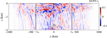
Figure 11. The HF part of the meridional velocity as a function of latitude and depth at a given time. The data are from run 3d-NT-
 $r_{3}$
. The locations
$r_{3}$
. The locations
 $\pm y_{m}=\pm 400$
km are the measurement locations where meridional fluxes are calculated and plotted in figure 12.
$\pm y_{m}=\pm 400$
km are the measurement locations where meridional fluxes are calculated and plotted in figure 12.
Allowing the jet to develop in 3d and spawn eddies, the solution looks significantly different. A snapshot of the HF part of the meridional velocity
 $v^{HF}$
is plotted in figure 11. The asymmetry between north and south does not appear as clearly as it does in the zonally uniform runs. The propagation is away from the storm track but not predominantly towards the equator. Due to eddy interactions, the characteristics along which NIW energy is radiated are not easily discernible in the upper ocean. Indeed, the primary effect of turbulent geostrophic flow on NIWs is scattering of the waves, leading to a redistribution of their energy in wavenumber space (Danioux & Vanneste Reference Danioux and Vanneste2016). Near-inertial waves generated in cyclones with
$v^{HF}$
is plotted in figure 11. The asymmetry between north and south does not appear as clearly as it does in the zonally uniform runs. The propagation is away from the storm track but not predominantly towards the equator. Due to eddy interactions, the characteristics along which NIW energy is radiated are not easily discernible in the upper ocean. Indeed, the primary effect of turbulent geostrophic flow on NIWs is scattering of the waves, leading to a redistribution of their energy in wavenumber space (Danioux & Vanneste Reference Danioux and Vanneste2016). Near-inertial waves generated in cyclones with
 $\unicode[STIX]{x1D714}=f_{eff}>f$
can propagate poleward provided that they enter less cyclonic (or even anticyclonic) regions.
$\unicode[STIX]{x1D714}=f_{eff}>f$
can propagate poleward provided that they enter less cyclonic (or even anticyclonic) regions.
The presumed poleward propagation is confirmed by quantifying the meridional flux
 $F(y,z)$
at both latitudes
$F(y,z)$
at both latitudes
 $y=\pm y_{m}$
, which is plotted in figure 12(a). Surprisingly, both equatorward and poleward fluxes have the same order of magnitude. The flux ratio is 0.6, i.e. 15 times larger than the flux ratio calculated in run 2d-NT-
$y=\pm y_{m}$
, which is plotted in figure 12(a). Surprisingly, both equatorward and poleward fluxes have the same order of magnitude. The flux ratio is 0.6, i.e. 15 times larger than the flux ratio calculated in run 2d-NT-
 $r_{3}$
. We conclude that allowing the zonal jet to meander and to expel mesoscale eddies increases the poleward propagation of NIWs tremendously. Furthermore, zonally averaged surface spectra are plotted in figure 12(b) at both latitudes
$r_{3}$
. We conclude that allowing the zonal jet to meander and to expel mesoscale eddies increases the poleward propagation of NIWs tremendously. Furthermore, zonally averaged surface spectra are plotted in figure 12(b) at both latitudes
 $y=\pm y_{m}$
to compare poleward and equatorward propagation. The southern spectrum has a peak at the mid-domain frequency
$y=\pm y_{m}$
to compare poleward and equatorward propagation. The southern spectrum has a peak at the mid-domain frequency
 $f_{0}$
while the northern spectrum has a peak centred at frequency
$f_{0}$
while the northern spectrum has a peak centred at frequency
 $\unicode[STIX]{x1D714}_{{>}f_{0}}$
. As expected, the energies contained in both peaks have comparable magnitudes. In the north, super-inertial energy is contained in a continuous range of frequencies, and a significant amount of it can travel up to 1000 km poleward.
$\unicode[STIX]{x1D714}_{{>}f_{0}}$
. As expected, the energies contained in both peaks have comparable magnitudes. In the north, super-inertial energy is contained in a continuous range of frequencies, and a significant amount of it can travel up to 1000 km poleward.
Figure 12. (a) Time-averaged meridional fluxes at fixed latitudes
 $y_{m}=\pm 400$
km. The data are from run 3d-NT-
$y_{m}=\pm 400$
km. The data are from run 3d-NT-
 $r_{3}$
. (b) Zonally averaged surface frequency spectra computed at latitudes
$r_{3}$
. (b) Zonally averaged surface frequency spectra computed at latitudes
 $\pm y_{m}$
. The data are from run 3d-NT-
$\pm y_{m}$
. The data are from run 3d-NT-
 $r_{3}$
. The spectra computed at latitudes
$r_{3}$
. The spectra computed at latitudes
 $-y_{m}$
and
$-y_{m}$
and
 $y_{m}$
are indicated respectively with grey and black solid lines. The vertical black and grey lines are respectively
$y_{m}$
are indicated respectively with grey and black solid lines. The vertical black and grey lines are respectively
 $\unicode[STIX]{x1D714}=f_{0}+\unicode[STIX]{x1D6FD}y_{m}$
and
$\unicode[STIX]{x1D714}=f_{0}+\unicode[STIX]{x1D6FD}y_{m}$
and
 $\unicode[STIX]{x1D714}=f_{0}-\unicode[STIX]{x1D6FD}y_{m}$
. The peak of the southern spectrum is very near
$\unicode[STIX]{x1D714}=f_{0}-\unicode[STIX]{x1D6FD}y_{m}$
. The peak of the southern spectrum is very near
 $\unicode[STIX]{x1D714}=f_{0}$
. The peak of the northern spectrum is a continuous range of frequencies from
$\unicode[STIX]{x1D714}=f_{0}$
. The peak of the northern spectrum is a continuous range of frequencies from
 $f_{0}+\unicode[STIX]{x1D6FD}y_{m}$
to
$f_{0}+\unicode[STIX]{x1D6FD}y_{m}$
to
 $f_{0}+\unicode[STIX]{x1D6FD}\times 1000$
km. The vertical dashed lines are from left to right
$f_{0}+\unicode[STIX]{x1D6FD}\times 1000$
km. The vertical dashed lines are from left to right
 $\unicode[STIX]{x1D714}=f_{0}+\unicode[STIX]{x1D6FD}y$
for
$\unicode[STIX]{x1D714}=f_{0}+\unicode[STIX]{x1D6FD}y$
for
 $y=0,750,1000$
km.
$y=0,750,1000$
km.
4 Interpretation of the results
Our objective here is to explain how the presence of the meandering unstable jet and eddies enables the excitation of super-inertial waves that are not seen when the eddies are absent and the jet is zonally uniform. We begin by adopting a simplified linear viewpoint and noting that waves that propagate away from their source region must satisfy the linear dispersion relation that is embedded in the Sturm–Liouville problem.
4.1 Radiating waves satisfy the linear dispersion relation
Let us consider propagating waves far from the storm track, e.g. measured at latitude
 $\pm y_{m}$
outside of the excitation region. They have frequency, horizontal and vertical scales that satisfy the dispersion relation defined by the well-known Sturm–Liouville eigenvalue problem (e.g. Winters & D’Asaro Reference Winters and D’Asaro1997),
$\pm y_{m}$
outside of the excitation region. They have frequency, horizontal and vertical scales that satisfy the dispersion relation defined by the well-known Sturm–Liouville eigenvalue problem (e.g. Winters & D’Asaro Reference Winters and D’Asaro1997),
 $$\begin{eqnarray}\displaystyle {\displaystyle \frac{\text{d}}{\text{d}^{2}z}}{\hat{w}}_{m}(z)+(k_{m}^{2}+l_{m}^{2}){\displaystyle \frac{N(z)^{2}-\unicode[STIX]{x1D714}^{2}}{f^{2}-\unicode[STIX]{x1D714}^{2}}}{\hat{w}}_{m}(z) & = & \displaystyle 0.\end{eqnarray}$$
Here, we use the
 $f$
-plane approximation, assuming that the inhomogeneities of the medium occur at scales much larger than the wave itself. Indeed, the horizontal scales of NIWs are
$f$
-plane approximation, assuming that the inhomogeneities of the medium occur at scales much larger than the wave itself. Indeed, the horizontal scales of NIWs are
 $O(10{-}80)$
km in our simulations, and the slopes of the isopycnals are almost horizontal (see figure 4) at locations
$O(10{-}80)$
km in our simulations, and the slopes of the isopycnals are almost horizontal (see figure 4) at locations
 $y_{m}=\pm 400$
km, so that the terms
$y_{m}=\pm 400$
km, so that the terms
 $\unicode[STIX]{x2202}_{y}N$
and the
$\unicode[STIX]{x2202}_{y}N$
and the
 $\unicode[STIX]{x1D6FD}y$
can be neglected in the equations of motion.
$\unicode[STIX]{x1D6FD}y$
can be neglected in the equations of motion.
In (4.1),
 $m$
is the vertical mode number,
$m$
is the vertical mode number,
 $k_{m}$
and
$k_{m}$
and
 $l_{m}$
are respectively the zonal and meridional wavenumbers associated with
$l_{m}$
are respectively the zonal and meridional wavenumbers associated with
 $m$
, and
$m$
, and
 $\unicode[STIX]{x1D714}$
is the eigenfrequency. The terms
$\unicode[STIX]{x1D714}$
is the eigenfrequency. The terms
 ${\hat{w}}_{m}$
are the eigenfunctions of the eigenvalue problem, which describe the vertical velocity field
${\hat{w}}_{m}$
are the eigenfunctions of the eigenvalue problem, which describe the vertical velocity field
 $w$
. The equation is written under the TA, NT effects being small, as we concluded in § 3. Moreover, the wave field present in simulation 2d-NT-
$w$
. The equation is written under the TA, NT effects being small, as we concluded in § 3. Moreover, the wave field present in simulation 2d-NT-
 $r_{3}$
is well represented by (4.1) (not shown). In what follows, we anticipate the ocean frequency response based on the wave spatial scale selection process.
$r_{3}$
is well represented by (4.1) (not shown). In what follows, we anticipate the ocean frequency response based on the wave spatial scale selection process.
4.1.1 On a proposed selection process for the spatial scales of wind-driven waves
Gill (Reference Gill1984) developed a modal formalism for describing the subsequent excitation of sub-mixed layer motions and showed that the energy projects predominantly on the lowest vertical modes. This has been observed by, e.g., Chen, Reid & Nowlin (Reference Chen, Reid and Nowlin1996), Chant (Reference Chant2001) and Alford (Reference Alford2003) for local wind-driven waves. A projection of kinetic energy flux onto normal modes using (4.1) shows that approximately
 $80\,\%$
of the kinetic energy flux is contained in the first five vertical modes for run 2d-NT-
$80\,\%$
of the kinetic energy flux is contained in the first five vertical modes for run 2d-NT-
 $r_{3}$
, and confirms therefore a low-mode response.
$r_{3}$
, and confirms therefore a low-mode response.
The wind stress (imposed through the body force terms
 ${\mathcal{F}}_{u}$
and
${\mathcal{F}}_{u}$
and
 ${\mathcal{F}}_{v}$
) has a finite extent
${\mathcal{F}}_{v}$
) has a finite extent
 $L_{0}$
in the meridional direction. The meridional wavenumber decomposition of the wind stress can be understood by analogy with a Fourier transform of a localized Gaussian signal with variance
$L_{0}$
in the meridional direction. The meridional wavenumber decomposition of the wind stress can be understood by analogy with a Fourier transform of a localized Gaussian signal with variance
 $L_{0}$
. Therefore, the largest response is at meridional wavenumber
$L_{0}$
. Therefore, the largest response is at meridional wavenumber
 $l=0$
, and we expect large horizontal scales to dominate the spectrum. The rate of spectral decay, and thus the relative importance of smaller scales, will depend on the width of the localized signal
$l=0$
, and we expect large horizontal scales to dominate the spectrum. The rate of spectral decay, and thus the relative importance of smaller scales, will depend on the width of the localized signal
 $L_{0}$
. Because
$L_{0}$
. Because
 $L_{0}=100$
km is quite large in our simulations, we expect low-horizontal-wavenumber propagating waves. Later, we will see that additional horizontal scales smaller than
$L_{0}=100$
km is quite large in our simulations, we expect low-horizontal-wavenumber propagating waves. Later, we will see that additional horizontal scales smaller than
 $L_{0}$
are established by the flow itself and may contribute to excite waves with larger horizontal wavenumbers.
$L_{0}$
are established by the flow itself and may contribute to excite waves with larger horizontal wavenumbers.
4.1.2 Frequency response
In principle, zonal and meridional winds provide a wide range of frequencies at which the ocean could respond. Indeed, as discussed previously, both components of the wind forcing are white between
 $f_{s}=f_{0}-\unicode[STIX]{x1D6FD}L_{y}/2$
and
$f_{s}=f_{0}-\unicode[STIX]{x1D6FD}L_{y}/2$
and
 $f_{n}=f_{0}+\unicode[STIX]{x1D6FD}L_{y}/2$
. However, the frequencies of propagating waves generated in the storm track should match low vertical mode number
$f_{n}=f_{0}+\unicode[STIX]{x1D6FD}L_{y}/2$
. However, the frequencies of propagating waves generated in the storm track should match low vertical mode number
 $m$
and small horizontal wavenumber
$m$
and small horizontal wavenumber
 $K_{m}=\sqrt{k_{m}^{2}+l_{m}^{2}}$
, as suggested above. According to the Sturm–Liouville problem (4.1), the ocean response is a narrow near-inertial peak centred at frequency
$K_{m}=\sqrt{k_{m}^{2}+l_{m}^{2}}$
, as suggested above. According to the Sturm–Liouville problem (4.1), the ocean response is a narrow near-inertial peak centred at frequency
 $f_{0}$
.
$f_{0}$
.
4.2 Excitation mechanisms for super-inertial waves
The imposed HF wind forcing can excite super-inertial internal waves in two ways. First, the flow can act to shift the lower frequency limit for internal waves and produce super-inertial waves on the poleward side of the zonal jet. Super-inertial waves can also be excited if they are forced over smaller horizontal scales. To illustrate these two mechanisms, an additional set of simplified 2d experiments were run.
4.2.1 Presence of cyclonic shear
An approximate dispersion relation for NIWs propagating in a geostrophic shear flow was derived by Kunze (Reference Kunze1985) assuming that the horizontal spatial scale of the waves is comparable to the scale of the geostrophic flow and that their frequency is close to inertial. Under these approximations, the relative geostrophic vorticity
 $\unicode[STIX]{x1D701}$
acts to shift the lower bound of the internal waveband from the planetary value of the Coriolis frequency
$\unicode[STIX]{x1D701}$
acts to shift the lower bound of the internal waveband from the planetary value of the Coriolis frequency
 $f$
to an effective Coriolis frequency
$f$
to an effective Coriolis frequency
 $f_{eff}=f+\unicode[STIX]{x1D701}/2$
. For wind-driven low-mode waves with
$f_{eff}=f+\unicode[STIX]{x1D701}/2$
. For wind-driven low-mode waves with
 $l\ll m$
, the waves excited in such a scenario will have a near-inertial peak at
$l\ll m$
, the waves excited in such a scenario will have a near-inertial peak at
 $f_{eff}>f$
and are thus able to propagate poleward until they reach their critical latitude.
$f_{eff}>f$
and are thus able to propagate poleward until they reach their critical latitude.
To illustrate this effect, we contrast a pair of idealized 2d runs that differ slightly from all other runs discussed in this paper in that the initial density stratification is independent of latitude, i.e. with
 $\unicode[STIX]{x1D70C}_{s}=\unicode[STIX]{x1D70C}_{n}$
. The only difference between the two runs is the value of the target mean speed used to compute the forcing coefficient
$\unicode[STIX]{x1D70C}_{s}=\unicode[STIX]{x1D70C}_{n}$
. The only difference between the two runs is the value of the target mean speed used to compute the forcing coefficient
 $A_{u}$
and, as a result, the magnitude of the ambient cyclonic vorticity in the poleward portion of the wind-forced region.
$A_{u}$
and, as a result, the magnitude of the ambient cyclonic vorticity in the poleward portion of the wind-forced region.
When the target speed is set to
 $u_{0}$
, the north–south flux ratio is 0.1, indicating relatively little excitation of super-inertial waves. Doubling the target speed to
$u_{0}$
, the north–south flux ratio is 0.1, indicating relatively little excitation of super-inertial waves. Doubling the target speed to
 $2u_{o}$
, however, increases this ratio to 0.25. With increased ambient vorticity, a larger fraction of the waves excited have frequencies near
$2u_{o}$
, however, increases this ratio to 0.25. With increased ambient vorticity, a larger fraction of the waves excited have frequencies near
 $f_{eff}>f_{0}$
, and thus there is an increases in the fraction of poleward wave energy flux. As the scales
$f_{eff}>f_{0}$
, and thus there is an increases in the fraction of poleward wave energy flux. As the scales
 $u_{0}$
and
$u_{0}$
and
 $L_{0}$
for this simple demonstration are comparable to those in the more complicated simulation we are attempting to interpret, these results demonstrate the utility of the simple Kunze (Reference Kunze1985) dispersion relation in the advective–refractive regime of the simulation of primary interest. We also note that modifying the ambient vorticity by a factor of two does not substantially affect the overall wind work, as indicated by the remotely measured total wave energy flux.
$L_{0}$
for this simple demonstration are comparable to those in the more complicated simulation we are attempting to interpret, these results demonstrate the utility of the simple Kunze (Reference Kunze1985) dispersion relation in the advective–refractive regime of the simulation of primary interest. We also note that modifying the ambient vorticity by a factor of two does not substantially affect the overall wind work, as indicated by the remotely measured total wave energy flux.
4.2.2 Presence of small horizontal scales
For the lowest vertical wave modes, excitation of smaller horizontal scales implies propagating waves at higher frequencies. A simple way of introducing smaller horizontal scales in the problem is to shrink the meridional extent of the storm track
 $L_{0}$
. Indeed, when
$L_{0}$
. Indeed, when
 $L_{0}$
becomes small yet remains finite, the relative importance of smaller scales in the forcing increases. Again, we contrast a pair of idealized 2d runs similar to the previous ones, but we remove the background vorticity by setting
$L_{0}$
becomes small yet remains finite, the relative importance of smaller scales in the forcing increases. Again, we contrast a pair of idealized 2d runs similar to the previous ones, but we remove the background vorticity by setting
 $A_{u}=0$
. The two runs differ only in the width of the storm track
$A_{u}=0$
. The two runs differ only in the width of the storm track
 $L_{0}$
.
$L_{0}$
.
We observe that the north–south flux ratio is 0.04 for the relatively wide forcing region with
 $L_{0}=100$
km, while it reaches
$L_{0}=100$
km, while it reaches
 $0.34$
for the case with a narrower forcing region with
$0.34$
for the case with a narrower forcing region with
 $L_{0}=10$
km. Reducing the storm track width by a factor of 10 increases the relative importance of smaller horizontal scales in the forcing, increases the frequency of the internal waves excited and thus increases the relative importance of poleward NIW radiation. In this example, the effect is substantial: the north–south flux ratio increases by a factor of 8.5.
$L_{0}=10$
km. Reducing the storm track width by a factor of 10 increases the relative importance of smaller horizontal scales in the forcing, increases the frequency of the internal waves excited and thus increases the relative importance of poleward NIW radiation. In this example, the effect is substantial: the north–south flux ratio increases by a factor of 8.5.
4.3 Super-inertial waves radiating poleward from a storm track
We now have all of the elements required to understand the significant increase in poleward internal wave radiation when the zonal jet is allowed to go unstable, meander and shed eddies. In steady state, the effective width of the jet is reduced and its ambient vorticity is increased relative to the artificially constrained zonally uniform simulation (see figure 6). The poleward frequency response in the 3d problem is a near-inertial peak that is broader than the corresponding peak towards the equator (see figure 12). Excitation at frequencies higher than
 $f_{0}$
produces poleward propagating low-mode waves that escape the generation region. The super-inertial excitation results from the ambient cyclonic vorticity that becomes established on the poleward side of the meandering jet over horizontal scales that are finite but significantly smaller than the width of the storm track.
$f_{0}$
produces poleward propagating low-mode waves that escape the generation region. The super-inertial excitation results from the ambient cyclonic vorticity that becomes established on the poleward side of the meandering jet over horizontal scales that are finite but significantly smaller than the width of the storm track.
The effectiveness of ambient vorticity in shifting the excitation frequency of waves depends on both the magnitude of the ambient vorticity itself and the meridional horizontal length scale over which the vorticity is present. For example, a very small region of significantly enhanced ambient vorticity will not produce a significant poleward flux because the surface area of such a region is too small to extract significant work from the wind. For waves at a given observed super-inertial frequency, there are two potential mechanisms for their generation. The first is direct excitation at
 $f_{eff}$
, assuming that the region over which
$f_{eff}$
, assuming that the region over which
 $f_{eff}$
exists is large enough that low-mode waves are constrained to be very near
$f_{eff}$
exists is large enough that low-mode waves are constrained to be very near
 $f_{eff}$
by the dispersion relationship. The second is direct excitation over a smaller region characterized by higher ambient vorticity. Owing to the smaller horizontal scale at which this excitation occurs, the dispersion relation requires that low-mode waves be excited with an additional frequency shift beyond that induced by the ambient vorticity. These two mechanisms act together to produce a relatively broad near- but super-inertial frequency response well poleward of the excitation region.
$f_{eff}$
by the dispersion relationship. The second is direct excitation over a smaller region characterized by higher ambient vorticity. Owing to the smaller horizontal scale at which this excitation occurs, the dispersion relation requires that low-mode waves be excited with an additional frequency shift beyond that induced by the ambient vorticity. These two mechanisms act together to produce a relatively broad near- but super-inertial frequency response well poleward of the excitation region.
Within the storm track, the relationship between the ambient vorticity and the associated surface area is determined by the nonlinear dynamics of the forced, meandering and eddy-shedding jet. This in turn controls the interplay between the two mechanisms of § 4.2, the width of the poleward near-inertial peak in figure 12 and the north–south flux ratio of the radiating NIWs.
5 Summary and discussion
The wind blowing on the ocean surface generates oceanic motions with a large range of frequencies. One part of the kinetic energy is contained in LF motions, mesoscale currents and eddies, which are strongly constrained by the Earth’s rotation to follow the balance between the Coriolis and the pressure gradient forces. Winds also create NIWs, which are HF and unbalanced motions with frequencies close to the inertial frequency
 $f=2\unicode[STIX]{x1D6FA}\sin \unicode[STIX]{x1D719}$
. Both dynamics have been considered in the present problem using high-resolution numerical simulations solving the Boussinesq equations on the
$f=2\unicode[STIX]{x1D6FA}\sin \unicode[STIX]{x1D719}$
. Both dynamics have been considered in the present problem using high-resolution numerical simulations solving the Boussinesq equations on the
 $\unicode[STIX]{x1D6FD}$
-plane.
$\unicode[STIX]{x1D6FD}$
-plane.
Because the storm track region is horizontally quite widespread, the HF wind excites low-vertical-mode (Gill Reference Gill1984) waves at large horizontal scale. To satisfy the dispersion relation, the frequency content of those waves is near-inertial at mid-domain frequency
 $f_{0}$
. This problem has been refined for realism by (i) incorporating the NT Coriolis force in the equations of motion and (ii) relaxing the zonally uniform constraint allowing the zonal jet to become baroclinically unstable, to meander and to expel mesoscale eddies.
$f_{0}$
. This problem has been refined for realism by (i) incorporating the NT Coriolis force in the equations of motion and (ii) relaxing the zonally uniform constraint allowing the zonal jet to become baroclinically unstable, to meander and to expel mesoscale eddies.
On the
 $\unicode[STIX]{x1D6FD}$
-plane, retaining the NT Coriolis force modifies the dispersion relation of internal waves. In particular, linear theory shows that NIWs are able to propagate poleward of their inertial latitude and can be focused and trapped in the deep weakly stratified ocean. This phenomenon is observed in our NT zonally uniform experiment, where new paths guide sub-inertial energy in weakly stratified deep ocean, increasing by 33
$\unicode[STIX]{x1D6FD}$
-plane, retaining the NT Coriolis force modifies the dispersion relation of internal waves. In particular, linear theory shows that NIWs are able to propagate poleward of their inertial latitude and can be focused and trapped in the deep weakly stratified ocean. This phenomenon is observed in our NT zonally uniform experiment, where new paths guide sub-inertial energy in weakly stratified deep ocean, increasing by 33
 $\,\%$
the poleward near-inertial propagation. Even so, most near-inertial energy propagates equatorward and NT effects remain weak.
$\,\%$
the poleward near-inertial propagation. Even so, most near-inertial energy propagates equatorward and NT effects remain weak.
After relaxing the zonally uniform constraint, the propagation becomes almost equally distributed between north and south. This propagation is due to both near-inertial and super-inertial excitation. The latter results from the combined effect of the presence of significant cyclonic shear and small horizontal scales. The two mechanisms of § 4.2 become significant in the 3d problem because the baroclinically unstable zonal jet thins compared with its zonally uniform counterpart, creating higher values of vertical vorticity in a relatively small region. Therefore, in addition to shifting the inertial frequency, the meandering jet introduces horizontal scales smaller than the scale of the storm track itself. Both mechanisms act together to enhance near- but super-inertial wave excitation and poleward radiation, comparable to equatorward radiation.
We have presented here a new mechanism by which an LF turbulent zonal jet modifies the propagation of NIWs excited by HF winds significantly. Even though theory and observations have suggested that the propagation of wind-driven internal waves is mainly towards the equator, Alford (Reference Alford2003) has observed poleward propagation in the North Pacific and North Equatorial Atlantic Oceans.
Acknowledgements
M.T. received funding through the G. Unger Vetlesen Foundation and K.B.W. was supported by the National Science Foundation (grant number OCE-1061027). XSEDE and NCAR/CISL computing resources were made available respectively under NSF grant number TG-OCE120004 and NCAR educational grant number NCAR0246.


