


1 Introduction
Turbulent heat and mass transport processes are important in various engineering situations. For example, heat transport problems are concerned with heat exchangers, whereas mass transport phenomena are found in air pollutant dispersion. In general situations, a turbulent velocity field generates fluctuations in a scalar field via turbulent convection, and the fluctuating scalar field conversely affects the velocity field by local forces due to changes in temperature or mass concentration. Assuming that the variation of temperature or mass is small enough in a way that does not affect the velocity field, it is then considered that the scalar field is passively convected by the velocity field. Such a scalar is sometimes called a ‘passive scalar’ and is the object of this study.
Heat and mass transport processes are controlled by the Prandtl number  $Pr=\unicode[STIX]{x1D708}/\unicode[STIX]{x1D6FC}$ and the Schmidt number
  $Sc=\unicode[STIX]{x1D708}/\unicode[STIX]{x1D705}$, respectively, where
  $\unicode[STIX]{x1D708}$ is the kinematic viscosity,
  $\unicode[STIX]{x1D6FC}$ is the thermal diffusivity and
  $\unicode[STIX]{x1D705}$ is the mass diffusivity. The Prandtl number takes a value of approximately 0.71 for air at atmospheric pressure and
  $27\,^{\circ }\text{C}$,
  $Pr\approx 0.871{-}13.6$ for water (H2O),
  $Pr\approx 100{-}50\,000$ for engine oils and
  $Pr\approx 0.003{-}0.03$ for liquid metals (Eckert & Drake Reference Eckert and Drake1959). The value of the Schmidt number, on the other hand, lies typically in the range of 0.2 to 4 for gas–gas diffusive systems at standard conditions, whereas
  $Sc\approx 200{-}1500$ for gas–liquid and liquid–liquid diffusive systems. Since both the Prandtl and Schmidt numbers range widely from small to large values in our surroundings, it is of great importance to clarify the parameter dependence of turbulent scalar transport over a broad range of the Schmidt number (or the Prandtl number).
It has been known that the statistical properties of passive scalar fluctuations transported by the turbulent velocity field vary significantly depending on the Reynolds number and Schmidt number. Such a variation is found, for example, in the scalar variance spectrum in homogeneous isotropic turbulence (see Gotoh, Watanabe & Suzuki Reference Gotoh, Watanabe and Suzuki2011; Gotoh & Yeung Reference Gotoh, Yeung, Davidson, Kaneda and Sreenivasan2012; Sreenivasan Reference Sreenivasan2018). When the Reynolds number is sufficiently high, the asymptotic scalar variance spectrum has the form  $k^{-17/3}$ in the inertial-diffusive range for
  $Sc\ll 1$,
  $k^{-5/3}$ in the inertial-convective range for
  $Sc=O(1)$, and
  $k^{-1}$ in the viscous-convective range for
  $Sc\gg 1$ (Obukhov Reference Obukhov1949; Corrsin Reference Corrsin1951; Batchelor Reference Batchelor1959; Batchelor, Howells & Townsend Reference Batchelor, Howells and Townsend1959). These power-law scalings have been studied extensively by early laboratory experiments (e.g., Sreenivasan Reference Sreenivasan1996; Mydlarski & Warhaft Reference Mydlarski and Warhaft1998) and direct numerical simulations (DNS) (e.g., Watanabe & Gotoh Reference Watanabe and Gotoh2004, Reference Watanabe and Gotoh2007; Gotoh, Watanabe & Miura Reference Gotoh, Watanabe and Miura2014; Yeung & Sreenivasan Reference Yeung and Sreenivasan2014; Gotoh & Watanabe Reference Gotoh and Watanabe2015).
Since widely varying the Reynolds and Schmidt numbers results in the diversity of turbulently mixed states of a passive scalar and their corresponding statistics, it is meaningful to find a suitable control parameter upon which passive scalar statistics is systematically dependent, if any. The aim of this study is to demonstrate that the Péclet number based on the Taylor microscale of scalar fluctuation, defined in (2.15), works as such a control parameter. In passive scalar turbulence, there exist multiple characteristic length scales of velocity and scalar fluctuations. Having multiple choices of length scales, one can define the Péclet number using a characteristic length scale of velocity fluctuation (cf. (2.15)). Note here that characteristic length scales of scalar fluctuation vary relative to those of velocity fluctuation and the system size depending on the existing control parameters and injection methods of velocity and scalar fluctuations. Accounting for this variation may be one of the key ingredients to suitably characterise different turbulently mixed states of a passive scalar. One successful example of this is found in the work by Lepore & Mydlarski (Reference Lepore and Mydlarski2012), who investigated higher-order scalar structure functions for two different scalar fields generated in two ways: heated cylinder and mandoline. They found that, although the scalar (temperature) is convected by an identical turbulent flow, the value of the thermal integral length scale differs between heated cylinder and mandoline, which results in the different values of the Péclet number based on this length scale. When plotted against the Péclet-number-compensated separation, which takes into account the variation of the thermal integral length scale, the higher-order scalar structure functions collapse at small scales for the two different scalar fields (Lepore & Mydlarski Reference Lepore and Mydlarski2012).
In this study, we investigate parameter dependencies of small-scale statistics of scalar fluctuations convected by statistically stationary homogeneous isotropic turbulence, considering the effect of variations of length scales of turbulence. Scalar fluctuations therein are sustained under a uniform mean scalar gradient. We focus especially on the small-scale anisotropy of scalar fluctuations appearing in this flow system. It has been reported that, in turbulent flows with a mean scalar gradient, the skewness of scalar derivative fluctuations in the direction of the mean gradient becomes non-zero (Sreenivasan & Tavoularis Reference Sreenivasan and Tavoularis1980; Budwig, Tavoularis & Corrsin Reference Budwig, Tavoularis and Corrsin1985; Sreenivasan Reference Sreenivasan1991; Holzer & Siggia Reference Holzer and Siggia1994; Tong & Warhaft Reference Tong and Warhaft1994; Mydlarski & Warhaft Reference Mydlarski and Warhaft1998; Warhaft Reference Warhaft2000; Yeung, Xu & Sreenivasan Reference Yeung, Xu and Sreenivasan2002; Schumacher, Sreenivasan & Yeung Reference Schumacher, Sreenivasan and Yeung2003; Yeung et al. Reference Yeung, Xu, Donzis and Sreenivasan2004; Yeung, Donzis & Sreenivasan Reference Yeung, Donzis and Sreenivasan2005; Donzis & Yeung Reference Donzis and Yeung2010; Yeung & Sreenivasan Reference Yeung and Sreenivasan2014), and it has still remained unsettled whether or not the small-scale scalar anisotropy can persist over a wide range of parameter values.
In order to achieve the aim mentioned above, we undertake an exhaustive parametric DNS study. We conduct DNS of passive scalar turbulence with 59 different combinations of Reynolds and Schmidt numbers. Since we change the values of these numbers herein, the velocity and scalar characteristic length scales vary accordingly although the scalar injection method is fixed. We discuss the parameter dependences of scalar statistics based on our DNS data. In § 2, we describe numerical methods and parameters used to simulate passive scalar turbulence. The results of the present study are shown in § 3, and our conclusion and discussion are presented in § 4.
2 Governing equations and numerical simulations
In the present study, we perform DNS of a passive scalar advected by statistically stationary homogeneous isotropic turbulence under a uniform mean scalar gradient. Under a triply periodic boundary condition ( $0\leqslant x_{1},x_{2},x_{3}<2\unicode[STIX]{x03C0}$), we solve the incompressible Navier–Stokes equations
 $$\begin{eqnarray}\displaystyle \frac{\unicode[STIX]{x2202}\boldsymbol{u}}{\unicode[STIX]{x2202}t}+(\boldsymbol{u}\boldsymbol{\cdot }\unicode[STIX]{x1D735})\boldsymbol{u}=-\frac{1}{\unicode[STIX]{x1D70C}}\unicode[STIX]{x1D735}p+\unicode[STIX]{x1D708}\unicode[STIX]{x1D6FB}^{2}\boldsymbol{u}+\boldsymbol{f},\quad \unicode[STIX]{x1D735}\boldsymbol{\cdot }\boldsymbol{u}=0, & & \displaystyle\end{eqnarray}$$
 where  $\boldsymbol{u}(\boldsymbol{x},t)$,
  $p(\boldsymbol{x},t)$ and
  $\boldsymbol{f}(\boldsymbol{x},t)$ are the velocity, pressure and external forcing fields, respectively, and fluid density
  $\unicode[STIX]{x1D70C}$ is assumed to be constant. In order to generate statistically stationary isotropic turbulence, we use the white Gaussian isotropic force
  $\boldsymbol{f}(\boldsymbol{x},t)$, which is defined in Fourier space as
 $$\begin{eqnarray}\displaystyle \overline{\widehat{f}_{i}(\boldsymbol{k},t)}=0,\quad \overline{\widehat{f}_{i}(\boldsymbol{k},t)\widehat{f}_{j}(-\boldsymbol{k},s)}=P_{ij}(\boldsymbol{k})\frac{W(k)}{4\unicode[STIX]{x03C0}k^{2}}\unicode[STIX]{x1D6FF}(t-s), & & \displaystyle\end{eqnarray}$$
 where  $P_{ij}(\boldsymbol{k})=\unicode[STIX]{x1D6FF}_{ij}-k_{i}k_{j}/k^{2}$ is a projection operator,
  $\unicode[STIX]{x1D6FF}_{ij}$ is the Kronecker delta,
  $\unicode[STIX]{x1D6FF}(\cdot )$ is the Dirac delta function and
  $\overline{(\cdot )}$ and
  $\widehat{(\cdot )}$ denote a time average and the Fourier coefficient of
  $(\cdot )$, respectively. Here,
  $W(k)$ is set to a constant value of 0.3 for the forcing wavenumber range
  $8\leqslant |\boldsymbol{k}|\leqslant 9$, otherwise,
  $W(k)=0$. With respect to a passive scalar, we decompose the scalar concentration
  $\unicode[STIX]{x1D6E9}(\boldsymbol{x},t)$ into mean and fluctuation parts as
  $\unicode[STIX]{x1D6E9}(\boldsymbol{x},t)=\overline{\unicode[STIX]{x1D6E9}}(\boldsymbol{x})+\unicode[STIX]{x1D703}(\boldsymbol{x},t)$. For sustaining scalar fluctuations, we impose a uniform mean scalar gradient in the
  $x_{3}$-direction as
  $\unicode[STIX]{x1D735}\overline{\unicode[STIX]{x1D6E9}}=(0,0,\unicode[STIX]{x1D6E4})$, where
  $\unicode[STIX]{x1D6E4}$ is the magnitude of the gradient and is set to unity without loss of generality. We thereby solve the following governing equation for
  $\unicode[STIX]{x1D703}(\boldsymbol{x},t)$:
 $$\begin{eqnarray}\displaystyle \frac{\unicode[STIX]{x2202}}{\unicode[STIX]{x2202}t}\unicode[STIX]{x1D703}+(\boldsymbol{u}\boldsymbol{\cdot }\unicode[STIX]{x1D735})\unicode[STIX]{x1D703}=\unicode[STIX]{x1D705}\unicode[STIX]{x1D6FB}^{2}\unicode[STIX]{x1D703}-\unicode[STIX]{x1D6E4}u_{3}, & & \displaystyle\end{eqnarray}$$
in conjunction with (2.1).
The energy spectrum,  $E_{u}(k,t)$, is computed by integrating the energy spectral density
  $Q_{u}(\boldsymbol{k},t)=\frac{1}{2}\widehat{u}_{i}(\boldsymbol{k},t)\widehat{u}_{i}(-\boldsymbol{k},t)$ over a spherical surface in
  $\boldsymbol{k}$-space as
 $$\begin{eqnarray}\displaystyle E_{u}(k,t)=\int _{0}^{2\unicode[STIX]{x03C0}}\,\text{d}\unicode[STIX]{x1D713}\int _{0}^{\unicode[STIX]{x03C0}}\,\text{d}\unicode[STIX]{x1D719}k^{2}\sin \unicode[STIX]{x1D719}Q_{u}(\boldsymbol{k},t). & & \displaystyle\end{eqnarray}$$
 The scalar variance spectrum,  $E_{\unicode[STIX]{x1D703}}(k,t)$, is similarly computed as
 $$\begin{eqnarray}\displaystyle E_{\unicode[STIX]{x1D703}}(k,t)=\int _{0}^{2\unicode[STIX]{x03C0}}\,\text{d}\unicode[STIX]{x1D713}\int _{0}^{\unicode[STIX]{x03C0}}\,\text{d}\unicode[STIX]{x1D719}k^{2}\sin \unicode[STIX]{x1D719}Q_{\unicode[STIX]{x1D703}}(\boldsymbol{k},t), & & \displaystyle\end{eqnarray}$$
 where  $Q_{\unicode[STIX]{x1D703}}(\boldsymbol{k},t)=\widehat{\unicode[STIX]{x1D703}}(\boldsymbol{k},t)\widehat{\unicode[STIX]{x1D703}}(-\boldsymbol{k},t)$ is the scalar variance spectral density. Using these spectra, the total kinetic energy and scalar variance per unit mass are computed, respectively, as
 $$\begin{eqnarray}\displaystyle & \displaystyle {\textstyle \frac{1}{2}}\langle \boldsymbol{u}^{2}\rangle (t)={\textstyle \frac{3}{2}}u^{\prime }(t)^{2}=\int _{0}^{\infty }E_{u}(k,t)\,\text{d}k, & \displaystyle\end{eqnarray}$$
 $$\begin{eqnarray}\displaystyle & \displaystyle \langle \unicode[STIX]{x1D703}^{2}\rangle (t)=\unicode[STIX]{x1D703}^{\prime }(t)^{2}=\int _{0}^{\infty }E_{\unicode[STIX]{x1D703}}(k,t)\,\text{d}k, & \displaystyle\end{eqnarray}$$
 where  $\langle (\cdot )\rangle$ denotes the space average of
  $(\cdot )$ over the entire computational domain, and
  $u^{\prime }(t)$ and
  $\unicode[STIX]{x1D703}^{\prime }(t)$ are the space-averaged root mean squares of velocity and scalar fluctuations.
Here we introduce several characteristic length scales of turbulence. We define integral length scales of velocity and scalar fluctuations, respectively, as
 $$\begin{eqnarray}\displaystyle & \displaystyle L_{u}(t)=\frac{3\unicode[STIX]{x03C0}}{4}\frac{\displaystyle \int _{0}^{\infty }k^{-1}E_{u}(k,t)\,\text{d}k}{\displaystyle \int _{0}^{\infty }E_{u}(k,t)\,\text{d}k}, & \displaystyle\end{eqnarray}$$
 $$\begin{eqnarray}\displaystyle & \displaystyle L_{\unicode[STIX]{x1D703}}(t)=\frac{\unicode[STIX]{x03C0}}{2}\frac{\displaystyle \int _{0}^{\infty }k^{-1}E_{\unicode[STIX]{x1D703}}(k,t)\,\text{d}k}{\displaystyle \int _{0}^{\infty }E_{\unicode[STIX]{x1D703}}(k,t)\,\text{d}k}. & \displaystyle\end{eqnarray}$$
The Taylor microscales of velocity and scalar fluctuations are computed, respectively, by
 $$\begin{eqnarray}\displaystyle & \displaystyle \unicode[STIX]{x1D706}_{u}(t)=\sqrt{\frac{15\unicode[STIX]{x1D708}u^{\prime }(t)^{2}}{\unicode[STIX]{x1D716}(t)}}, & \displaystyle\end{eqnarray}$$
 $$\begin{eqnarray}\displaystyle & \displaystyle \unicode[STIX]{x1D706}_{\unicode[STIX]{x1D703}}(t)=\sqrt{\frac{6\unicode[STIX]{x1D705}\unicode[STIX]{x1D703}^{\prime }(t)^{2}}{\unicode[STIX]{x1D712}(t)}}, & \displaystyle\end{eqnarray}$$
 where the energy dissipation rate  $\unicode[STIX]{x1D716}(t)$ and the scalar dissipation rate
  $\unicode[STIX]{x1D712}(t)$ per unit mass are computed as
  $\unicode[STIX]{x1D716}(t)=\unicode[STIX]{x1D708}/2\langle (\unicode[STIX]{x2202}u_{i}/\unicode[STIX]{x2202}x_{j}+\unicode[STIX]{x2202}u_{j}/\unicode[STIX]{x2202}x_{i})^{2}\rangle$ and
  $\unicode[STIX]{x1D712}(t)=2\unicode[STIX]{x1D705}\langle (\unicode[STIX]{x2202}\unicode[STIX]{x1D703}/\unicode[STIX]{x2202}x_{i})^{2}\rangle$, respectively. The Kolmogorov scale,
  $\unicode[STIX]{x1D702}_{K}(t)$, and the Batchelor scale,
  $\unicode[STIX]{x1D702}_{B}(t)$, are defined as
 $$\begin{eqnarray}\displaystyle & \unicode[STIX]{x1D702}_{K}(t)=\unicode[STIX]{x1D708}^{3/4}\unicode[STIX]{x1D716}(t)^{-1/4}, & \displaystyle\end{eqnarray}$$
 $$\begin{eqnarray}\displaystyle & \unicode[STIX]{x1D702}_{B}(t)=\unicode[STIX]{x1D705}^{1/2}\unicode[STIX]{x1D708}^{1/4}\unicode[STIX]{x1D716}(t)^{-1/4}=\unicode[STIX]{x1D702}_{K}(t)Sc^{-1/2}. & \displaystyle\end{eqnarray}$$
 We discuss our results using the Reynolds number  $Re_{\unicode[STIX]{x1D706}}(t)$ based on
  $\unicode[STIX]{x1D706}_{u}(t)$ and the Péclet number
  $Pe_{\unicode[STIX]{x1D706}_{\unicode[STIX]{x1D703}}}(t)$ based on
  $\unicode[STIX]{x1D706}_{\unicode[STIX]{x1D703}}(t)$, which are, respectively, written as
 $$\begin{eqnarray}\displaystyle & \displaystyle Re_{\unicode[STIX]{x1D706}}(t)=\frac{u^{\prime }(t)\unicode[STIX]{x1D706}_{u}(t)}{\unicode[STIX]{x1D708}}, & \displaystyle\end{eqnarray}$$
 $$\begin{eqnarray}\displaystyle & \displaystyle Pe_{\unicode[STIX]{x1D706}_{\unicode[STIX]{x1D703}}}(t)=\frac{u^{\prime }(t)\unicode[STIX]{x1D706}_{\unicode[STIX]{x1D703}}(t)}{\unicode[STIX]{x1D705}}. & \displaystyle\end{eqnarray}$$
 Instead of the Péclet number thus defined,  $Pe_{\unicode[STIX]{x1D706}}(t)=ScRe_{\unicode[STIX]{x1D706}}(t)=u^{\prime }(t)\unicode[STIX]{x1D706}_{u}(t)/\unicode[STIX]{x1D705}$ is sometimes used in the literature. As will be discussed, however, equation (2.15) is more appropriate in characterising the small-scale scalar statistics for various Reynolds and Schmidt numbers.
Setting moderate forcing wavenumbers ( $8\leqslant |\boldsymbol{k}|\leqslant 9$) in (2.2) effectively improves the isotropy of the velocity field. The
  $(2\unicode[STIX]{x03C0})^{3}$ periodic domain becomes significantly larger than the integral length scale
  $\overline{L}_{u}$ of the velocity. See table 1 for the quantitative information about the isotropic flows of four different Reynolds numbers (
 $\overline{Re}_{\unicode[STIX]{x1D706}}\approx 7$, 29, 63 and 106). Denoting one side of the triply periodic box by
  $L_{box}$ (
 $=2\unicode[STIX]{x03C0}$),
  $L_{box}/\overline{L}_{u}$ is 22.2, 21.7, 27.2 and 29.6 at
  $\overline{Re}_{\unicode[STIX]{x1D706}}\approx 7$, 29, 63 and 106, respectively. In this numerical set-up, a large number of eddies of various orientations, the size of which is comparable to
  $\overline{L}_{u}$, are contained in the computational domain, whereby even an instantaneous velocity field becomes reasonably isotropic on space average. Here, the degree of isotropy of velocity fluctuations is evaluated in terms of values of
  $\overline{u_{2}^{\prime 2}}/\overline{u_{1}^{\prime 2}}$ and
  $\overline{u_{3}^{\prime 2}}/\overline{u_{1}^{\prime 2}}$, both of which are very close to unity (thus velocity fluctuations being isotropic) for the four different Reynolds numbers (see table 1). One should keep in mind that, although the random forcing (2.2) is delta correlated in time, the velocity field has a finite correlation time of the order of
  $T_{L}$, where
  $T_{L}=\overline{L}_{u}/\overline{u^{\prime }}$ is the large-eddy turnover time. Using larger forcing wavenumbers, we can reduce the effect of the finite correlation time such that it becomes shorter (relative to
  $L_{box}/\overline{u^{\prime }}$) and the fluctuations of global quantities for velocity field are more attenuated. The latter is found in table 1 such that the ratio
  $\unicode[STIX]{x1D70E}_{u^{\prime 2}}/\overline{u^{\prime 2}}$ takes small values of the order of
  $10^{-2}$, where
  $\unicode[STIX]{x1D70E}_{u^{\prime 2}}$ is the temporal standard deviation of
  $u^{\prime }(t)^{2}$. One of the important advantages of using moderate forcing wavenumbers is that it improves the sampling for small-scale statistics of scalar fluctuations albeit at the cost of a reduced inertial range. It also allows scalar structures to grow significantly larger than
  $\overline{L}_{u}$, as will be demonstrated in § 3.1. The velocity-derivative skewness
  $\overline{S}_{u}=\overline{\langle (\unicode[STIX]{x2202}u_{1}/\unicode[STIX]{x2202}x_{1})^{3}\rangle /\langle (\unicode[STIX]{x2202}u_{1}/\unicode[STIX]{x2202}x_{1})^{2}\rangle ^{3/2}}$ is
  $-0.00637$,
  $-0.342$,
  $-0.502$ and
  $-0.525$ at
  $\overline{Re}_{\unicode[STIX]{x1D706}}\approx 7$, 29, 63 and 106, respectively (table 1). The velocity field at
  $\overline{Re}_{\unicode[STIX]{x1D706}}\approx 7$ is far from being turbulent. Nonetheless, the velocity field evolves in a spatio-temporally random manner because of the random forcing (2.2), thereby mixing a passive scalar.
Table 1. Velocity statistics of DNS with the four different values of  $\unicode[STIX]{x1D708}$. Here,
  $Re_{\unicode[STIX]{x1D706}}$ is the Reynolds number based on the Taylor microscale (2.14),
  $L_{u}$ is the integral length scale (2.8),
  $\unicode[STIX]{x1D706}_{u}$ is the Taylor microscale (2.10),
  $\unicode[STIX]{x1D702}_{K}$ is the Kolmogorov microscale (2.12),
  $S_{u}$ is the velocity-derivative skewness. The velocity statistics of labels A, B, C and D are, respectively, computed using runs A1, B1, C1 and D1 shown in tables 2 and 3.

In the present study, DNS is performed using the pseudo-spectral method and the fourth-order Runge–Kutta–Gill method (see Gotoh et al. (Reference Gotoh, Watanabe and Suzuki2011), for further details). We have run long-term numerical simulations at the four different Reynolds numbers ( $\overline{Re}_{\unicode[STIX]{x1D706}}\approx 7$, 29, 63, 106) while varying the Schmidt number. We use 59 different combinations of
  $\unicode[STIX]{x1D708}$ and
  $Sc$, where the lowest and highest
  $Sc$ used are
  $1/4096$ and 256, respectively (see tables 2 and 3). When
  $Sc\ll 1$, it is necessary to make the time resolution finer to resolve the scalar diffusion time scale that becomes much shorter than the advection time scales. We also need to allocate the number of numerical grid points,
  $N^{3}$, such that both the Kolmogorov scale (2.12) and the Batchelor scale (2.13) are well resolved. When
  $Sc$ is unity, the Kolmogorov scale equals the Batchelor scale (i.e.,
  $\overline{\unicode[STIX]{x1D702}}_{K}=\overline{\unicode[STIX]{x1D702}}_{B}$). At a fixed Reynolds number, however,
  $\overline{\unicode[STIX]{x1D702}}_{B}$ becomes smaller with increasing
  $Sc$ so that
  $N^{3}$ must be increased accordingly (Yeung et al. Reference Yeung, Xu, Donzis and Sreenivasan2004; Donzis & Yeung Reference Donzis and Yeung2010; Gotoh, Hatanaka & Miura Reference Gotoh, Hatanaka and Miura2012). In the present study, we use a reasonable spatial resolution for each simulation;
  $k_{max}\overline{\unicode[STIX]{x1D702}}_{B}$ is at worse equal to 1.24 for run A256 (see table 2), where the cutoff wavenumber
  $k_{max}=\sqrt{2}N/3$ (Gotoh & Yeung Reference Gotoh, Yeung, Davidson, Kaneda and Sreenivasan2012). For computing turbulence statistics in a statistically stationary state, time averages are taken over the time period of
  $T_{av}$ which excludes the initial transient period of time. Here,
  $T_{av}$ is at worse equal to 4.19
  $T_{L}$ for run D1024i (see table 3).
Table 2. Parameters and scalar statistics of DNS with various values of  $Sc$ for
  $\unicode[STIX]{x1D708}=0.01$ (series-A) and 0.003 (series-B). Here,
  $\unicode[STIX]{x1D708}$ is the kinematic viscosity,
  $Sc$ is the Schmidt number,
  $N^{3}$ is the number of numerical grid points,
  $\unicode[STIX]{x0394}t$ is the time increment,
  $Pe_{\unicode[STIX]{x1D706}_{\unicode[STIX]{x1D703}}}$ is the Péclet number based on the Taylor microscale of scalar fluctuation (2.15),
  $S_{\unicode[STIX]{x2202}\unicode[STIX]{x1D703}/\unicode[STIX]{x2202}x_{3}}$ is the scalar derivative skewness (3.1),
  $F_{\unicode[STIX]{x2202}\unicode[STIX]{x1D703}/\unicode[STIX]{x2202}x_{3}}$ is the scalar derivative flatness (3.2),
  $g_{\unicode[STIX]{x1D703}}$ is the ratio of parallel-to-perpendicular scalar-gradient variances (3.3),
  $a$ is the anisotropy parameter (3.4),
  $k_{max}\unicode[STIX]{x1D702}_{B}$ is the spatial resolution,
  $T_{av}$ is the time period for computing statistics in the unit of large-eddy turnover time,
  $T_{L}$.

Table 3. Parameters and scalar statistics of DNS with various values of  $Sc$ for
  $\unicode[STIX]{x1D708}=8\times 10^{-4}$ (series-C) and
  $3\times 10^{-4}$ (series-D). The description of the parameters and statistics shown is found in the caption of table 2.

3 Results
3.1 Scalar variance spectra and flow visualisations
Figure 1(a) shows the variation of the time-averaged scalar variance spectrum  $\overline{E}_{\unicode[STIX]{x1D703}}(k)$ for decreasing
  $Sc$ at the highest Reynolds number
  $\overline{Re}_{\unicode[STIX]{x1D706}}\approx 106$. Here,
  $\overline{E}_{\unicode[STIX]{x1D703}}(k)$ exhibits the power-law scalings slightly shallower than
  $k^{-5/3}$ for
  $Sc=1$ and than
  $k^{-17/3}$ for
  $Sc=1/1024$ (Yeung & Sreenivasan Reference Yeung and Sreenivasan2013, Reference Yeung and Sreenivasan2014). Batchelor et al. (Reference Batchelor, Howells and Townsend1959) analytically derived the
  $k^{-17/3}$ power-law scaling for the turbulent scalar fluctuation field, which is locally isotropic. We show below, however, the case in which the scalar fluctuation field is significantly anisotropic when the power-law scaling slightly shallower than
  $k^{-17/3}$ emerges in the scalar variance spectrum. There is a peculiar tendency that, at
  $Sc=1/1024$,
  $\overline{E}_{\unicode[STIX]{x1D703}}(k)$ increases significantly with decreasing
  $k$ for
  $k\leqslant 7$. This tendency is partially described by the shape of the energy spectrum at
  $\overline{Re}_{\unicode[STIX]{x1D706}}\approx 106$. Figure 1(b) shows
  $\overline{E}_{u}(k)$ and multiplied energy spectrum
  $k^{-4}\overline{E}_{u}(k)$ at
  $\overline{Re}_{\unicode[STIX]{x1D706}}\approx 106$. Note that Batchelor et al. (Reference Batchelor, Howells and Townsend1959) theoretically derived
  $\overline{E}_{\unicode[STIX]{x1D703}}(k)=(\unicode[STIX]{x1D712}/3\unicode[STIX]{x1D705}^{3})k^{-4}\overline{E}_{u}(k)$ for
  $Sc\ll 1$. Here,
  $k^{-4}\overline{E}_{u}(k)$ is an increasing function with decreasing
  $k$ for
  $k\leqslant 7$, as similarly observed in
  $\overline{E}_{\unicode[STIX]{x1D703}}(k)$. Therefore, for
  $Sc\ll 1$, the scalar variance spectrum
  $\overline{E}_{\unicode[STIX]{x1D703}}(k)$ can be related to the multiplied energy spectrum
  $k^{-4}\overline{E}_{u}(k)$. Incidentally, we find that the velocity-scalar cospectrum shows the power-law scaling slightly shallower than
  $k^{-11/3}$ in the inertial-diffusive range at low Schmidt numbers and
  $\overline{Re}_{\unicode[STIX]{x1D706}}\approx 106$ (data not shown). The
  $k^{-11/3}$ power-law scaling was theoretically derived by O’Gorman & Pullin (Reference O’Gorman and Pullin2005).

Figure 1. (a) Time-averaged scalar variance spectra  $\overline{E}_{\unicode[STIX]{x1D703}}(k)$ with three different Schmidt numbers at
  $\overline{Re}_{\unicode[STIX]{x1D706}}\approx 106$. The red, blue and black curves correspond to
  $Sc=1$,
  $1/64$ and
  $1/1024$, respectively. (b) Time-averaged energy spectra
  $k^{\unicode[STIX]{x1D6FC}}\overline{E}_{u}(k)$, at
  $\overline{Re}_{\unicode[STIX]{x1D706}}\approx 106$. The red and black curves correspond to
  $\unicode[STIX]{x1D6FC}=0$ and
  $\unicode[STIX]{x1D6FC}=-4$, respectively. The dashed black, red and blue lines denote the
  $k^{-5/3}$,
  $k^{-17/3}$ and
  $k^{2}$ power-law slopes, respectively.

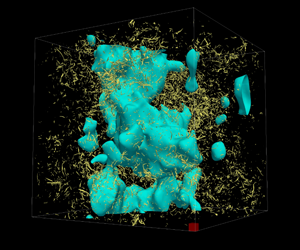
Figure 2. Visualisations of instantaneous flow fields of passive scalar turbulence with a uniform mean scalar gradient. Yellow isosurfaces denote high enstrophy. Cyan isosurfaces denote scalar fluctuation ( $\unicode[STIX]{x1D703}<0$). Here,
  $\overline{Re}_{\unicode[STIX]{x1D706}}\approx 106$. One side of the small red cube placed in the bottom right-hand corner of the periodic domain is the integral length scale
  $\overline{L}_{u}$ of velocity fluctuation. (a) Run D1,
  $Sc=1$ and
  $\overline{Pe}_{\unicode[STIX]{x1D706}_{\unicode[STIX]{x1D703}}}=57.0$; (b) run D64i,
  $Sc=1/64$ and
  $\overline{Pe}_{\unicode[STIX]{x1D706}_{\unicode[STIX]{x1D703}}}=6.15$; (c) run D1024i,
  $Sc=1/1024$ and
  $\overline{Pe}_{\unicode[STIX]{x1D706}_{\unicode[STIX]{x1D703}}}=1.06$.
Figure 2 shows the visualisations of the instantaneous enstrophy and scalar fluctuation fields with three different Schmidt numbers ( $Sc=1,1/64,1/1024$), at
  $\overline{Re}_{\unicode[STIX]{x1D706}}\approx 106$. We find an interesting feature that scalar fluctuation structures visualised by cyan isosurfaces become larger for decreasing
  $Sc$. At the lowest Schmidt number (
 $Sc=1/1024$), anomalous large-scale anisotropic scalar structures emerge from the isotropic turbulent velocity field (figure 2c). These structures are elongated along the direction of the mean scalar gradient, and their size is significantly large (cf. Schumacher, Sreenivasan & Yeung Reference Schumacher, Sreenivasan and Yeung2005). This size is visually evident by comparison with the size of the red cube at the right-hand bottom corner, one side of which is
  $\overline{L}_{u}$ (figure 2c). Quantitative evidence for this is shown in figure 3 in terms of the variations of
  $\overline{L}_{\unicode[STIX]{x1D703}}/\overline{L}_{u}$ and
  $\overline{\unicode[STIX]{x1D706}}_{\unicode[STIX]{x1D703}}/\overline{L}_{u}$ with respect to
  $\overline{Pe}_{\unicode[STIX]{x1D706}_{\unicode[STIX]{x1D703}}}$. In accordance with our visualisation (figure 2), the scalar characteristic length scales
  $\overline{L}_{\unicode[STIX]{x1D703}}$ and
  $\overline{\unicode[STIX]{x1D706}}_{\unicode[STIX]{x1D703}}$ increase compared to
  $\overline{L}_{u}$ with decreasing
  $\overline{Pe}_{\unicode[STIX]{x1D706}_{\unicode[STIX]{x1D703}}}$. For
  $\overline{Re}_{\unicode[STIX]{x1D706}}\approx 106$,
  $\overline{L}_{\unicode[STIX]{x1D703}}/\overline{L}_{u}$ and
  $\overline{\unicode[STIX]{x1D706}}_{\unicode[STIX]{x1D703}}/\overline{L}_{u}$ reach approximately 6 and 2.5, respectively, at
  $\overline{Pe}_{\unicode[STIX]{x1D706}_{\unicode[STIX]{x1D703}}}=1.06$. Overall, similar variations of
  $\overline{L}_{\unicode[STIX]{x1D703}}/\overline{L}_{u}$ and
  $\overline{\unicode[STIX]{x1D706}}_{\unicode[STIX]{x1D703}}/\overline{L}_{u}$ with respect to
  $\overline{Pe}_{\unicode[STIX]{x1D706}_{\unicode[STIX]{x1D703}}}$ are confirmed for all the Reynolds numbers shown (
 $\overline{Re}_{\unicode[STIX]{x1D706}}\approx 7$, 29, 63, 106). Note that, as seen in figure 2, we confirm a similar change of a scalar fluctuation field for decreasing
  $Sc$ and
  $\overline{Pe}_{\unicode[STIX]{x1D706}_{\unicode[STIX]{x1D703}}}$ at
  $\overline{Re}_{\unicode[STIX]{x1D706}}\approx 7$, 29, 63. Moreover, it is worth mentioning that no spontaneous formation of large-scale anisotropic scalar structures is identified when applying a white Gaussian scalar source (see Watanabe & Gotoh (Reference Watanabe and Gotoh2004), for details) instead of the uniform mean scalar gradient. This implies that the mean gradient is one of the key ingredients for the generation and sustenance of the large-scale anisotropic scalar structures (figure 2c).

Figure 3. The  $\overline{Pe}_{\unicode[STIX]{x1D706}_{\unicode[STIX]{x1D703}}}$-dependences of
  $\overline{L}_{\unicode[STIX]{x1D703}}/\overline{L}_{u}$ (a) and
  $\overline{\unicode[STIX]{x1D706}}_{\unicode[STIX]{x1D703}}/\overline{L}_{u}$ (b). Blue circles, black squares, green diamonds and red hexagons indicate the data for
  $\overline{Re}_{\unicode[STIX]{x1D706}}\approx 7$, 29, 63 and 106, respectively. Horizontal error bars denote the temporal standard deviations of
  $Pe_{\unicode[STIX]{x1D706}_{\unicode[STIX]{x1D703}}}(t)$ and vertical error bars denote those of
  $L_{\unicode[STIX]{x1D703}}(t)/\overline{L}_{u}$ (a) and
  $\unicode[STIX]{x1D706}_{\unicode[STIX]{x1D703}}(t)/\overline{L}_{u}$ (b). Both
  $\overline{L}_{\unicode[STIX]{x1D703}}/\overline{L}_{u}$ and
  $\overline{\unicode[STIX]{x1D706}}_{\unicode[STIX]{x1D703}}/\overline{L}_{u}$ show near constancy in the low Péclet number range because the scalar structures stop growing in size due to the domain size limit.
Here, the formation mechanism of the large-scale scalar structures when  $Sc\ll 1$ is explained as follows. First, blobs of mean scalar with amplitude of
  $O(\unicode[STIX]{x1D6E4}L_{f})$, where
  $L_{f}=2\unicode[STIX]{x03C0}/k_{f}$ and
  $k_{f}$ is the characteristic wavenumber of the forcing, are convected in the direction parallel to the mean scalar gradient by the velocity fluctuations of the scale
  $\overline{L}_{u}=O(L_{f})$. Once the convected scalar blobs meet, they quickly merge into larger blobs due to the large diffusivity with the time scale of
  $L_{f}^{2}/\unicode[STIX]{x1D705}$ (
 $\ll \overline{L}_{u}/\overline{u^{\prime }}=T_{L}$). Note that the fluid blobs do not merge due to the incompressibility. The convection and merging process of the scalar continue successively and selectively in the direction parallel to the mean scalar gradient, resulting in the formation of large-scale anisotropic scalar structures elongated in the direction of the mean gradient (figure 2c).
3.2 Dependences of scalar derivative statistics on  $Sc$ and $\overline{Pe}_{\unicode[STIX]{x1D706}_{\unicode[STIX]{x1D703}}}$


In figure 4, we show the well known scalar derivative statistics: the scalar derivative skewness and flatness, both of which have been investigated in the literature (Sreenivasan & Tavoularis Reference Sreenivasan and Tavoularis1980; Budwig et al. Reference Budwig, Tavoularis and Corrsin1985; Sreenivasan Reference Sreenivasan1991; Holzer & Siggia Reference Holzer and Siggia1994; Tong & Warhaft Reference Tong and Warhaft1994; Mydlarski & Warhaft Reference Mydlarski and Warhaft1998; Warhaft Reference Warhaft2000; Yeung et al. Reference Yeung, Xu and Sreenivasan2002; Schumacher et al. Reference Schumacher, Sreenivasan and Yeung2003; Yeung et al. Reference Yeung, Xu, Donzis and Sreenivasan2004, Reference Yeung, Donzis and Sreenivasan2005; Donzis & Yeung Reference Donzis and Yeung2010; Yeung & Sreenivasan Reference Yeung and Sreenivasan2014). In the present study, we compute the instantaneous skewness and flatness of  $\unicode[STIX]{x2202}\unicode[STIX]{x1D703}/\unicode[STIX]{x2202}x_{3}$, respectively, as
 $$\begin{eqnarray}\displaystyle & \displaystyle S_{\unicode[STIX]{x2202}\unicode[STIX]{x1D703}/\unicode[STIX]{x2202}x_{3}}(t)=\left.\left\langle \left(\frac{\unicode[STIX]{x2202}\unicode[STIX]{x1D703}}{\unicode[STIX]{x2202}x_{3}}-\left\langle \frac{\unicode[STIX]{x2202}\unicode[STIX]{x1D703}}{\unicode[STIX]{x2202}x_{3}}\right\rangle \right)^{3}\right\rangle \right/\!\left\langle \left(\frac{\unicode[STIX]{x2202}\unicode[STIX]{x1D703}}{\unicode[STIX]{x2202}x_{3}}-\left\langle \frac{\unicode[STIX]{x2202}\unicode[STIX]{x1D703}}{\unicode[STIX]{x2202}x_{3}}\right\rangle \right)^{2}\right\rangle ^{3/2}, & \displaystyle\end{eqnarray}$$
 $$\begin{eqnarray}\displaystyle & \displaystyle F_{\unicode[STIX]{x2202}\unicode[STIX]{x1D703}/\unicode[STIX]{x2202}x_{3}}(t)=\left.\left\langle \left(\frac{\unicode[STIX]{x2202}\unicode[STIX]{x1D703}}{\unicode[STIX]{x2202}x_{3}}-\left\langle \frac{\unicode[STIX]{x2202}\unicode[STIX]{x1D703}}{\unicode[STIX]{x2202}x_{3}}\right\rangle \right)^{4}\right\rangle \right/\!\left\langle \left(\frac{\unicode[STIX]{x2202}\unicode[STIX]{x1D703}}{\unicode[STIX]{x2202}x_{3}}-\left\langle \frac{\unicode[STIX]{x2202}\unicode[STIX]{x1D703}}{\unicode[STIX]{x2202}x_{3}}\right\rangle \right)^{2}\right\rangle ^{2}. & \displaystyle\end{eqnarray}$$
 In all the parameter cases, we confirm that both  $S_{\unicode[STIX]{x2202}\unicode[STIX]{x1D703}/\unicode[STIX]{x2202}x_{3}}(t)$ and
  $F_{\unicode[STIX]{x2202}\unicode[STIX]{x1D703}/\unicode[STIX]{x2202}x_{3}}(t)$ fluctuate around their most probable values beyond the initial transient period of time.

Figure 4. Skewness (a1,a2) and flatness (b1,b2) of scalar derivative  $\unicode[STIX]{x2202}\unicode[STIX]{x1D703}/\unicode[STIX]{x2202}x_{3}$ as functions of
  $Sc$ (a1,b1) and
  $\overline{Pe}_{\unicode[STIX]{x1D706}_{\unicode[STIX]{x1D703}}}$ (a2,b2). Blue circles, black squares, green diamonds and red hexagons indicate the data for
  $\overline{Re}_{\unicode[STIX]{x1D706}}\approx 7$, 29, 63 and 106, respectively. (a1,b1) Open blue inverted triangles,
  $\overline{Re}_{\unicode[STIX]{x1D706}}\approx 8$ from Yeung et al. (Reference Yeung, Xu, Donzis and Sreenivasan2004); open black triangles,
  $\overline{Re}_{\unicode[STIX]{x1D706}}\approx 38$ from Yeung et al. (Reference Yeung, Xu and Sreenivasan2002). (a2) Here,
  $\overline{S}_{\unicode[STIX]{x2202}\unicode[STIX]{x1D703}/\unicode[STIX]{x2202}x_{3}}$ becomes maximal at
  $\overline{Pe}_{\unicode[STIX]{x1D706}_{\unicode[STIX]{x1D703}}}\approx 20$ at each Reynolds number. Horizontal and vertical error bars denote the temporal standard deviations of the corresponding quantities.
Figures 4(a1) and 4(b1) demonstrate the dependences of  $\overline{S}_{\unicode[STIX]{x2202}\unicode[STIX]{x1D703}/\unicode[STIX]{x2202}x_{3}}$ and
  $\overline{F}_{\unicode[STIX]{x2202}\unicode[STIX]{x1D703}/\unicode[STIX]{x2202}x_{3}}$ on
  $Sc$, respectively, alongside the published data by Yeung et al. (Reference Yeung, Xu and Sreenivasan2002, Reference Yeung, Xu, Donzis and Sreenivasan2004). Our data and the published data of multiple
  $\overline{Re}_{\unicode[STIX]{x1D706}}$ demonstrate a qualitatively similar tendency. As
  $Sc$ is increased from a very low value,
  $\overline{S}_{\unicode[STIX]{x2202}\unicode[STIX]{x1D703}/\unicode[STIX]{x2202}x_{3}}$ first monotonically increases, and then decreases after reaching a peak (figure 4a1). Another important observation from figure 4(a1) is that, at
  $Sc=1$,
  $\overline{S}_{\unicode[STIX]{x2202}\unicode[STIX]{x1D703}/\unicode[STIX]{x2202}x_{3}}$ takes almost the same value (
 ${\approx}1.5$) at
  $\overline{Re}_{\unicode[STIX]{x1D706}}$, greater than or equal to 29. This observation is relevant to the persistence of non-zero derivative skewness of a passive scalar (Sreenivasan Reference Sreenivasan1991; Tong & Warhaft Reference Tong and Warhaft1994; Mydlarski & Warhaft Reference Mydlarski and Warhaft1998). The experiments of grid turbulence under a mean temperature gradient (Tong & Warhaft Reference Tong and Warhaft1994; Mydlarski & Warhaft Reference Mydlarski and Warhaft1998) demonstrated that the temperature derivative skewness takes a constant value of approximately 1.4 over a broad range of Reynolds number (up to
  $\overline{Re}_{\unicode[STIX]{x1D706}}\approx 731$), with the Prandtl number (or
  $Sc$) being of order unity.
  $\overline{F}_{\unicode[STIX]{x2202}\unicode[STIX]{x1D703}/\unicode[STIX]{x2202}x_{3}}$ is, on the other hand, a monotonically increasing function of
  $Sc$ for each Reynolds number (figure 4b1). The increase rate in
  $\overline{F}_{\unicode[STIX]{x2202}\unicode[STIX]{x1D703}/\unicode[STIX]{x2202}x_{3}}$ is observed to grow with increasing
  $\overline{Re}_{\unicode[STIX]{x1D706}}$.
Next, we compare plots of  $\overline{S}_{\unicode[STIX]{x2202}\unicode[STIX]{x1D703}/\unicode[STIX]{x2202}x_{3}}$ with respect to
  $Sc$ and
  $\overline{Pe}_{\unicode[STIX]{x1D706}_{\unicode[STIX]{x1D703}}}$ (figures 4a1 and 4a2). Although the variations of
  $\overline{S}_{\unicode[STIX]{x2202}\unicode[STIX]{x1D703}/\unicode[STIX]{x2202}x_{3}}$ with respect to
  $Sc$ do not collapse for different
  $\overline{Re}_{\unicode[STIX]{x1D706}}$ (figure 4a1), when plotted with respect to
  $\overline{Pe}_{\unicode[STIX]{x1D706}_{\unicode[STIX]{x1D703}}}$ the variations collapse well in the low
  $\overline{Pe}_{\unicode[STIX]{x1D706}_{\unicode[STIX]{x1D703}}}$ range (figure 4a2). We also confirm the dependence of
  $\overline{F}_{\unicode[STIX]{x2202}\unicode[STIX]{x1D703}/\unicode[STIX]{x2202}x_{3}}$ on
  $\overline{Pe}_{\unicode[STIX]{x1D706}_{\unicode[STIX]{x1D703}}}$ (figure 4b2). At much higher
  $\overline{Pe}_{\unicode[STIX]{x1D706}_{\unicode[STIX]{x1D703}}}$ than unity, the plots with respect to
  $\overline{Pe}_{\unicode[STIX]{x1D706}_{\unicode[STIX]{x1D703}}}$ for different
  $\overline{Re}_{\unicode[STIX]{x1D706}}$ do not collapse onto each other (see figure 4b2). In other words, the spatio-temporal intermittency of scalar fluctuations is sensitive to
  $\overline{Re}_{\unicode[STIX]{x1D706}}$ for
  $\overline{Pe}_{\unicode[STIX]{x1D706}_{\unicode[STIX]{x1D703}}}\gg 1$. The good agreement of plots for the four different
  $\overline{Re}_{\unicode[STIX]{x1D706}}$ in the low
  $\overline{Pe}_{\unicode[STIX]{x1D706}_{\unicode[STIX]{x1D703}}}$ range is due to the decoupling effect between velocity and scalar fluctuation fields, which is assessed in terms of mixed spectral skewness in § 3.4.
3.3 $\overline{Pe}_{\unicode[STIX]{x1D706}_{\unicode[STIX]{x1D703}}}$-dependence of small-scale anisotropy of scalar fluctuations

In order to evaluate the degree of small-scale anisotropy of scalar fluctuations, we compute the ratio of parallel-to-perpendicular scalar-gradient variances,  $g_{\unicode[STIX]{x1D703}}(t)$, defined as
 $$\begin{eqnarray}\displaystyle g_{\unicode[STIX]{x1D703}}(t)=\left.2\left\langle \frac{\unicode[STIX]{x2202}\unicode[STIX]{x1D703}}{\unicode[STIX]{x2202}x_{3}}\frac{\unicode[STIX]{x2202}\unicode[STIX]{x1D703}}{\unicode[STIX]{x2202}x_{3}}\right\rangle \right/\!\left[\left\langle \frac{\unicode[STIX]{x2202}\unicode[STIX]{x1D703}}{\unicode[STIX]{x2202}x_{1}}\frac{\unicode[STIX]{x2202}\unicode[STIX]{x1D703}}{\unicode[STIX]{x2202}x_{1}}\right\rangle +\left\langle \frac{\unicode[STIX]{x2202}\unicode[STIX]{x1D703}}{\unicode[STIX]{x2202}x_{2}}\frac{\unicode[STIX]{x2202}\unicode[STIX]{x1D703}}{\unicode[STIX]{x2202}x_{2}}\right\rangle \right]. & & \displaystyle\end{eqnarray}$$
Such a quantity has also been studied in the literature (Tong & Warhaft Reference Tong and Warhaft1994; Mydlarski & Warhaft Reference Mydlarski and Warhaft1998; Yeung & Sreenivasan Reference Yeung and Sreenivasan2014; Hill Reference Hill2017).
We also use the anisotropy parameter  $a(t)$ proposed by Hill (Reference Hill2017), defined as
 $$\begin{eqnarray}\displaystyle a(t)=\frac{F(t)+{\displaystyle \frac{\unicode[STIX]{x1D705}}{\unicode[STIX]{x1D705}_{T}(t)}}}{1+{\displaystyle \frac{\unicode[STIX]{x1D705}}{\unicode[STIX]{x1D705}_{T}(t)}}}, & & \displaystyle\end{eqnarray}$$
 where  $F(t)$ is defined as
 $$\begin{eqnarray}\displaystyle F(t)=\frac{g_{\unicode[STIX]{x1D703}}(t)-1}{g_{\unicode[STIX]{x1D703}}(t)+2}, & & \displaystyle\end{eqnarray}$$
 and  $\unicode[STIX]{x1D705}/\unicode[STIX]{x1D705}_{T}(t)$ is calculated using the eddy diffusivity
  $\unicode[STIX]{x1D705}_{T}(t)=\unicode[STIX]{x1D712}(t)/2\unicode[STIX]{x1D6E4}^{2}$ by
 $$\begin{eqnarray}\displaystyle \frac{\unicode[STIX]{x1D705}}{\unicode[STIX]{x1D705}_{T}(t)}=\frac{2\unicode[STIX]{x1D705}\unicode[STIX]{x1D6E4}^{2}}{\unicode[STIX]{x1D712}(t)}=\unicode[STIX]{x1D6E4}^{2}\!\left/\left\langle \frac{\unicode[STIX]{x2202}\unicode[STIX]{x1D703}}{\unicode[STIX]{x2202}x_{i}}\frac{\unicode[STIX]{x2202}\unicode[STIX]{x1D703}}{\unicode[STIX]{x2202}x_{i}}\right\rangle \right.=\left.\frac{\unicode[STIX]{x2202}\unicode[STIX]{x1D6E9}}{\unicode[STIX]{x2202}x_{3}}\frac{\unicode[STIX]{x2202}\unicode[STIX]{x1D6E9}}{\unicode[STIX]{x2202}x_{3}}\right/\!\left\langle \frac{\unicode[STIX]{x2202}\unicode[STIX]{x1D703}}{\unicode[STIX]{x2202}x_{i}}\frac{\unicode[STIX]{x2202}\unicode[STIX]{x1D703}}{\unicode[STIX]{x2202}x_{i}}\right\rangle . & & \displaystyle\end{eqnarray}$$
 Both  $g_{\unicode[STIX]{x1D703}}(t)$ and
  $F(t)$ relate to the small-scale anisotropy of scalar fluctuations, whereas
  $\unicode[STIX]{x1D705}/\unicode[STIX]{x1D705}_{T}(t)$ measures the macroscopic effect of the mean scalar gradient on scalar fluctuations. If small-scale scalar fluctuations become statistically isotropic, then
  $\overline{g}_{\unicode[STIX]{x1D703}}=1$ and
  $\overline{F}=0$ (note, however, that the opposite is not necessarily the case). The eddy diffusivity,
  $\unicode[STIX]{x1D705}_{T}(t)$, measures the strength of scalar mixing. The enhancement of mixing a passive scalar, therefore, results in the increase of
  $\unicode[STIX]{x1D705}_{T}(t)$ relative to
  $\unicode[STIX]{x1D705}$, i.e., the decrease of
  $\unicode[STIX]{x1D705}/\unicode[STIX]{x1D705}_{T}(t)$. One may expect that, when
  $\unicode[STIX]{x1D705}/\unicode[STIX]{x1D705}_{T}(t)$ is small, small-scale scalar fluctuations are isotropised due to the effective scalar mixing by the background isotropic flow. When
  $\unicode[STIX]{x1D705}/\unicode[STIX]{x1D705}_{T}(t)$ is large, on the other hand, small-scale gradients of scalar field do not develop but the strong molecular diffusion is balanced by the scalar excitations due to velocity fluctuations in the direction of the mean scalar gradient, wherein large-scale anisotropic scalar structures are formed (figure 2c). Here,
  $F(t)$ and
  $\unicode[STIX]{x1D705}/\unicode[STIX]{x1D705}_{T}(t)$ are contained in the anisotropic parameter
  $a(t)$ (3.4), where
  $a(t)$ is a measure of the ratio of the second-order coefficient (with a minus sign) to the zero-order coefficient in the Legendre expansion of shell-summed scalar variance spectral density (see Hill (Reference Hill2017), for details). When
  $\unicode[STIX]{x1D705}/\unicode[STIX]{x1D705}_{T}(t)\gg |F(t)|$ and
  $\unicode[STIX]{x1D705}/\unicode[STIX]{x1D705}_{T}(t)\gg 1$, both numerator and denominator of
  $a(t)$ are approximately equal to
  $\unicode[STIX]{x1D705}/\unicode[STIX]{x1D705}_{T}(t)$, which yields
  $a(t)\approx 1$; in other words, the second-order contribution in the Legendre expansion becomes almost as significant as the zero-order one. The scalar fluctuation field accordingly becomes an axisymmetric field that is highly affected by the mean scalar gradient (Hill Reference Hill2017).

Figure 5. The  $\overline{Pe}_{\unicode[STIX]{x1D706}_{\unicode[STIX]{x1D703}}}$-dependences of (a)
  $\overline{g}_{\unicode[STIX]{x1D703}}$, (b)
  $\overline{F}$, (c)
  $\unicode[STIX]{x1D705}/\overline{\unicode[STIX]{x1D705}}_{T}$ and (d)
  $\overline{a}$. Blue circles, black squares, green diamonds and red hexagons indicate data for
  $\overline{Re}_{\unicode[STIX]{x1D706}}\approx 7$, 29, 63 and 106, respectively. Horizontal and vertical error bars denote the temporal standard deviations of the corresponding quantities. (c) The black dashed line shows
  $\unicode[STIX]{x1D705}/\overline{\unicode[STIX]{x1D705}}_{T}\propto \overline{Pe}_{\unicode[STIX]{x1D706}_{\unicode[STIX]{x1D703}}}^{\,-2}$ (see appendix A for the derivation of the power-law scaling).
Figure 5 illustrates  $\overline{Pe}_{\unicode[STIX]{x1D706}_{\unicode[STIX]{x1D703}}}$-dependences of time-averaged values of the quantities introduced above (i.e.,
  $\overline{g}_{\unicode[STIX]{x1D703}}$,
  $\overline{F}$,
  $\unicode[STIX]{x1D705}/\overline{\unicode[STIX]{x1D705}}_{T}$,
  $\overline{a}$). The plots of
  $\overline{g}_{\unicode[STIX]{x1D703}}$ and
  $\overline{F}$ for the four different
  $\overline{Re}_{\unicode[STIX]{x1D706}}$ collapse well onto a single curve when arranged in terms of
  $\overline{Pe}_{\unicode[STIX]{x1D706}_{\unicode[STIX]{x1D703}}}$ (see figures 5a and 5b). There is a zero-crossing point of the curve of
  $\overline{F}$ at
  $\overline{Pe}_{\unicode[STIX]{x1D706}_{\unicode[STIX]{x1D703}}}\approx 7$. Below
  $\overline{Pe}_{\unicode[STIX]{x1D706}_{\unicode[STIX]{x1D703}}}\approx 7$, the scalar gradient fluctuations in the direction of the mean scalar gradient (i.e., vertical direction) become weaker than those in the directions perpendicular to it (horizontal directions), whereas those in the vertical direction become stronger than those in the horizontal directions above
  $\overline{Pe}_{\unicode[STIX]{x1D706}_{\unicode[STIX]{x1D703}}}\approx 7$. Above
  $\overline{Pe}_{\unicode[STIX]{x1D706}_{\unicode[STIX]{x1D703}}}\approx 20$, where
  $\overline{g}_{\unicode[STIX]{x1D703}}$ and
  $\overline{F}$ take their local maximal values, the dissipation-scale scalar fluctuations become less anisotropic with increasing
  $\overline{Pe}_{\unicode[STIX]{x1D706}_{\unicode[STIX]{x1D703}}}$, irrespective of
  $\overline{Re}_{\unicode[STIX]{x1D706}}$. As
  $\overline{Pe}_{\unicode[STIX]{x1D706}_{\unicode[STIX]{x1D703}}}$ increases, the effect of turbulent scalar mixing becomes more significant. Consequently, turbulent scalar mixing isotropises scalar fluctuations at dissipative scales.
In figures 5(a) and 5(b), we find that  $\overline{g}_{\unicode[STIX]{x1D703}}$ and
  $\overline{F}$ approach the values of 0.5 and
  $-0.2$, respectively, in the limit of
  $\overline{Pe}_{\unicode[STIX]{x1D706}_{\unicode[STIX]{x1D703}}}\rightarrow 0$. In this limit,
  $\overline{S}_{\unicode[STIX]{x2202}\unicode[STIX]{x1D703}/\unicode[STIX]{x2202}x_{3}}$ and
  $\overline{F}_{\unicode[STIX]{x2202}\unicode[STIX]{x1D703}/\unicode[STIX]{x2202}x_{3}}$ approach, respectively, the values of 0 and 3 (see figures 4a2 and 4b2). Hence, the probability density function (p.d.f.) of
  $\unicode[STIX]{x2202}\unicode[STIX]{x1D703}/\unicode[STIX]{x2202}x_{3}$ becomes approximately Gaussian; this is also the case for the p.d.f.s of
  $\unicode[STIX]{x2202}\unicode[STIX]{x1D703}/\unicode[STIX]{x2202}x_{1}$ and
  $\unicode[STIX]{x2202}\unicode[STIX]{x1D703}/\unicode[STIX]{x2202}x_{2}$ (figure not shown). At very low
  $\overline{Pe}_{\unicode[STIX]{x1D706}_{\unicode[STIX]{x1D703}}}$, the anisotropy of scalar fluctuation measured by
  $\overline{g}_{\unicode[STIX]{x1D703}}$ and
  $\overline{F}$ is maximal, which arises solely from the kinematic constraint on the velocity correlation function under the negligible effect of the convective term (see § 3.4). As
  $\overline{Pe}_{\unicode[STIX]{x1D706}_{\unicode[STIX]{x1D703}}}$ increases, the convective term affects the anisotropy in a way that makes the p.d.f. of
  $\unicode[STIX]{x2202}\unicode[STIX]{x1D703}/\unicode[STIX]{x2202}x_{3}$ positively skewed for moderate
  $\overline{Pe}_{\unicode[STIX]{x1D706}_{\unicode[STIX]{x1D703}}}$ and tends to recover its symmetry for high
  $\overline{Pe}_{\unicode[STIX]{x1D706}_{\unicode[STIX]{x1D703}}}$ (figure 4a2). It should be stressed that the second-order moment of fluctuation gives the width of the p.d.f., while the skewness, the third-order moment, measures the asymmetry of the p.d.f. Therefore, the anisotropy of the scalar gradients can exist even when their skewness is zero. Indeed, the fluctuations of the scalar gradients at very low
  $\overline{Pe}_{\unicode[STIX]{x1D706}_{\unicode[STIX]{x1D703}}}$ correspond to the anisotropic state with zero skewness, symmetric (almost Gaussian) p.d.f.s with different widths, while those at large
  $\overline{Pe}_{\unicode[STIX]{x1D706}_{\unicode[STIX]{x1D703}}}$ lead to nearly symmetric (non-Gaussian) p.d.f.s with almost the same widths, suggesting a nearly isotropic state.
Figure 5(c) shows the  $\overline{Pe}_{\unicode[STIX]{x1D706}_{\unicode[STIX]{x1D703}}}$-dependence of
  $\unicode[STIX]{x1D705}/\overline{\unicode[STIX]{x1D705}}_{T}$. Similarly to
  $\overline{g}_{\unicode[STIX]{x1D703}}$ and
  $\overline{F}$, the plots of
  $\unicode[STIX]{x1D705}/\overline{\unicode[STIX]{x1D705}}_{T}$ for the four different
  $\overline{Re}_{\unicode[STIX]{x1D706}}$ are found to collapse well onto a single curve. Here,
  $\unicode[STIX]{x1D705}/\overline{\unicode[STIX]{x1D705}}_{T}$ increases drastically with decreasing
  $\overline{Pe}_{\unicode[STIX]{x1D706}_{\unicode[STIX]{x1D703}}}$. The increasing behaviour follows
  $\unicode[STIX]{x1D705}/\overline{\unicode[STIX]{x1D705}}_{T}\propto \overline{Pe}_{\unicode[STIX]{x1D706}_{\unicode[STIX]{x1D703}}}^{\,-2}$ in the range of
  $\overline{Pe}_{\unicode[STIX]{x1D706}_{\unicode[STIX]{x1D703}}}\lesssim 1$, where
  $\overline{F}$ becomes a close to the asymptotic value of
  $-0.2$ (figure 5b). Note that the power law
  $\unicode[STIX]{x1D705}/\overline{\unicode[STIX]{x1D705}}_{T}\propto \overline{Pe}_{\unicode[STIX]{x1D706}_{\unicode[STIX]{x1D703}}}^{\,-2}$ can be derived with dimensional analysis (see appendix A). The slope observed above
  $\overline{Pe}_{\unicode[STIX]{x1D706}_{\unicode[STIX]{x1D703}}}\approx 5$ is shallower, which is attributed to the scalar transport by the velocity field. Finally, we note that the plots of the anisotropy parameter
  $\overline{a}$ for the four different
  $\overline{Re}_{\unicode[STIX]{x1D706}}$ also collapse well onto a single curve (see figure 5d). The effect of
  $\unicode[STIX]{x1D705}/\overline{\unicode[STIX]{x1D705}}_{T}$ in
  $\overline{a}$ becomes more manifest for decreasing
  $\overline{Pe}_{\unicode[STIX]{x1D706}_{\unicode[STIX]{x1D703}}}$. As
  $\overline{Pe}_{\unicode[STIX]{x1D706}_{\unicode[STIX]{x1D703}}}$ is decreased below
  $\overline{Pe}_{\unicode[STIX]{x1D706}_{\unicode[STIX]{x1D703}}}\approx 5$,
  $\unicode[STIX]{x1D705}/\overline{\unicode[STIX]{x1D705}}_{T}$ becomes significantly larger than
  $|\overline{F}|$ (i.e.,
  $\unicode[STIX]{x1D705}/\overline{\unicode[STIX]{x1D705}}_{T}\gg |\overline{F}|$); consequently,
  $\overline{a}$ approaches unity so that the second-order Legendre contribution is almost as significant as the zero-order one.
Based on figure 5, it is reasonable to consider that the variations of  $\overline{g}_{\unicode[STIX]{x1D703}}$,
  $\overline{F}$,
  $\unicode[STIX]{x1D705}/\overline{\unicode[STIX]{x1D705}}_{T}$ and
  $\overline{a}$ are characterised by universal functions of
  $\overline{Pe}_{\unicode[STIX]{x1D706}_{\unicode[STIX]{x1D703}}}$, and thus we conclude that
  $\overline{Pe}_{\unicode[STIX]{x1D706}_{\unicode[STIX]{x1D703}}}$ is a key parameter to determine the degree of small-scale anisotropy of scalar fluctuations under a uniform mean scalar gradient.
3.4 Asymptotic behaviour of scalar fluctuations as $\overline{Pe}_{\unicode[STIX]{x1D706}_{\unicode[STIX]{x1D703}}}\rightarrow 0$

Having found in figure 5(a) that the value of  $\overline{g}_{\unicode[STIX]{x1D703}}$ approaches 0.5 as
  $\overline{Pe}_{\unicode[STIX]{x1D706}_{\unicode[STIX]{x1D703}}}\rightarrow 0$, we further investigate the asymptotic behaviour of scalar fluctuations. Figure 6 shows mixed spectral skewness
  $S_{\unicode[STIX]{x1D703}}(t)$, computed as
 $$\begin{eqnarray}\displaystyle S_{\unicode[STIX]{x1D703}}(t)=\frac{2}{15}\frac{\displaystyle \int _{0}^{\infty }k^{2}T_{\unicode[STIX]{x1D703}}(k,t)\,\text{d}k}{(\unicode[STIX]{x1D716}(t)/15\unicode[STIX]{x1D708})^{1/2}(\unicode[STIX]{x1D712}(t)/6\unicode[STIX]{x1D705})}, & & \displaystyle\end{eqnarray}$$
 where  $T_{\unicode[STIX]{x1D703}}(k,t)$ is the scalar-variance transfer function appearing in the spectral equation for the scalar variance (see Watanabe & Gotoh (Reference Watanabe and Gotoh2004, Reference Watanabe and Gotoh2007), for details). Here,
  $S_{\unicode[STIX]{x1D703}}(t)$ is a measure of the degree of interaction between velocity and scalar fluctuation fields (Kerr Reference Kerr1985; Briard & Gomez Reference Briard and Gomez2016). Irrespective of the value of
  $\overline{Re}_{\unicode[STIX]{x1D706}}$,
  $-\overline{S}_{\unicode[STIX]{x1D703}}$ approaches zero with decreasing
  $\overline{Pe}_{\unicode[STIX]{x1D706}_{\unicode[STIX]{x1D703}}}$, where the effect of turbulent scalar mixing becomes insignificant (figure 6).

Figure 6. Time-averaged mixed spectral skewness  $-\overline{S}_{\unicode[STIX]{x1D703}}$ as a function of
  $\overline{Pe}_{\unicode[STIX]{x1D706}_{\unicode[STIX]{x1D703}}}$. Blue circles, black squares, green diamonds and red hexagons indicate data for
  $\overline{Re}_{\unicode[STIX]{x1D706}}\approx 7$, 29, 63 and 106, respectively. Horizontal error bars denote the temporal standard deviations of
  $Pe_{\unicode[STIX]{x1D706}_{\unicode[STIX]{x1D703}}}(t)$ and vertical error bars denote those of
  $-S_{\unicode[STIX]{x1D703}}(t)$.
Based on this behaviour of mixed spectral skewness, we next consider the asymptotic condition in Fourier space in the limit of  $\overline{Pe}_{\unicode[STIX]{x1D706}_{\unicode[STIX]{x1D703}}}\rightarrow 0$,
 $$\begin{eqnarray}\displaystyle \unicode[STIX]{x1D705}k^{2}\widehat{\unicode[STIX]{x1D703}}(\boldsymbol{k},t)\approx -\unicode[STIX]{x1D6E4}\widehat{u}_{3}(\boldsymbol{k},t), & & \displaystyle\end{eqnarray}$$
 where the time-derivative term and convective term are negligibly small. In order to assess its validity, we introduce the residual function,  $\widehat{\unicode[STIX]{x1D6E5}}(\boldsymbol{k},t)$, as
 $$\begin{eqnarray}\displaystyle \widehat{\unicode[STIX]{x1D6E5}}(\boldsymbol{k},t)=\widehat{\unicode[STIX]{x1D703}}(\boldsymbol{k},t)+\frac{\unicode[STIX]{x1D6E4}}{\unicode[STIX]{x1D705}k^{2}}\widehat{u}_{3}(\boldsymbol{k},t), & & \displaystyle\end{eqnarray}$$
 and consider the asymptotic behaviour of the spectrum  $E_{\unicode[STIX]{x1D6E5}}(k,t)$ of this function,
 $$\begin{eqnarray}\displaystyle E_{\unicode[STIX]{x1D6E5}}(k,t)=\int _{0}^{2\unicode[STIX]{x03C0}}\,\text{d}\unicode[STIX]{x1D713}\int _{0}^{\unicode[STIX]{x03C0}}\,\text{d}\unicode[STIX]{x1D719}k^{2}\sin \unicode[STIX]{x1D719}\widehat{\unicode[STIX]{x1D6E5}}(\boldsymbol{k},t)\widehat{\unicode[STIX]{x1D6E5}}(-\boldsymbol{k},t), & & \displaystyle\end{eqnarray}$$
 in comparison with  $E_{\unicode[STIX]{x1D703}}(k,t)$. If
  $E_{\unicode[STIX]{x1D6E5}}(k,t)\ll E_{\unicode[STIX]{x1D703}}(k,t)$, then (3.8) holds. Figure 7 shows the variation of the magnitude relationship between
  $\overline{E}_{\unicode[STIX]{x1D6E5}}(k)$ and
  $\overline{E}_{\unicode[STIX]{x1D703}}(k)$ with respect to
  $\overline{Pe}_{\unicode[STIX]{x1D706}_{\unicode[STIX]{x1D703}}}$, for
  $\overline{Re}_{\unicode[STIX]{x1D706}}\approx 69$. At moderate
  $\overline{Pe}_{\unicode[STIX]{x1D706}_{\unicode[STIX]{x1D703}}}$,
  $\overline{E}_{\unicode[STIX]{x1D6E5}}(k)$ is not negligible (see figures 7a and 7b) so that (3.8) is not applicable. As
  $\overline{Pe}_{\unicode[STIX]{x1D706}_{\unicode[STIX]{x1D703}}}$ is further decreased,
  $\overline{E}_{\unicode[STIX]{x1D6E5}}(k)$ tends to become smaller relative to
  $\overline{E}_{\unicode[STIX]{x1D703}}(k)$. As for run C4096i (figure 7d), in particular,
  $\overline{E}_{\unicode[STIX]{x1D6E5}}(k)$ is approximately two to three orders of magnitude smaller than
  $\overline{E}_{\unicode[STIX]{x1D703}}(k)$ at any wavenumber, meaning that (3.8) is valid. Note that such a tendency with respect to
  $\overline{Pe}_{\unicode[STIX]{x1D706}_{\unicode[STIX]{x1D703}}}$ is found for the other Reynolds numbers. The result above is numerical evidence for justifying that (3.8) is the asymptotic condition in the limit of
  $\overline{Pe}_{\unicode[STIX]{x1D706}_{\unicode[STIX]{x1D703}}}\rightarrow 0$.

Figure 7. Comparisons between  $\overline{E}_{\unicode[STIX]{x1D703}}(k)$ and
  $\overline{E}_{\unicode[STIX]{x1D6E5}}(k)$ at
  $\overline{Re}_{\unicode[STIX]{x1D706}}\approx 69$ and four different Schmidt numbers. (a) Run C1,
  $Sc=1$ and
  $\overline{Pe}_{\unicode[STIX]{x1D706}_{\unicode[STIX]{x1D703}}}=34.6$; (b) run C16i,
  $Sc=1/16$ and
  $\overline{Pe}_{\unicode[STIX]{x1D706}_{\unicode[STIX]{x1D703}}}=6.50$; (c) run C256i,
  $Sc=1/256$ and
  $\overline{Pe}_{\unicode[STIX]{x1D706}_{\unicode[STIX]{x1D703}}}=0.912$; (d) run C4096i,
  $Sc=1/4096$ and
  $\overline{Pe}_{\unicode[STIX]{x1D706}_{\unicode[STIX]{x1D703}}}=0.0742$.
Using (3.8), in the following, we analytically derive the asymptotic value of  $\overline{g}_{\unicode[STIX]{x1D703}}=0.5$ as
  $Pe_{\unicode[STIX]{x1D706}_{\unicode[STIX]{x1D703}}}\rightarrow 0$, as found in figure 5(a). Here, we may compute
  $\overline{g}_{\unicode[STIX]{x1D703}}$ as
 $$\begin{eqnarray}\displaystyle \overline{g}_{\unicode[STIX]{x1D703}}=\left.\overline{\iiint k_{3}^{2}|\widehat{\unicode[STIX]{x1D703}}|^{2}(\boldsymbol{k},t)\,\text{d}\boldsymbol{k}}\right/\overline{\iiint k_{1}^{2}|\widehat{\unicode[STIX]{x1D703}}|^{2}(\boldsymbol{k},t)\,\text{d}\boldsymbol{k}}. & & \displaystyle\end{eqnarray}$$
We calculate the numerator in (3.11) using (3.8) as
 $$\begin{eqnarray}\displaystyle \overline{\iiint k_{3}^{2}|\widehat{\unicode[STIX]{x1D703}}(\boldsymbol{k},t)|^{2}\,\text{d}\boldsymbol{k}} & {\approx} & \displaystyle \frac{\unicode[STIX]{x1D6E4}^{2}}{\unicode[STIX]{x1D705}^{2}}\iiint \frac{k_{3}^{2}}{k^{4}}\overline{|\widehat{u}_{3}|^{2}}(\boldsymbol{k})\,\text{d}\boldsymbol{k}\nonumber\\ \displaystyle & = & \displaystyle \frac{\unicode[STIX]{x1D6E4}^{2}}{\unicode[STIX]{x1D705}^{2}}\iiint \frac{k_{3}^{2}}{k^{4}}P_{33}(\boldsymbol{k})\overline{Q_{u}^{\ast }}(k)\,\text{d}\boldsymbol{k}\nonumber\\ \displaystyle & = & \displaystyle \frac{8\unicode[STIX]{x03C0}}{15}\frac{\unicode[STIX]{x1D6E4}^{2}}{\unicode[STIX]{x1D705}^{2}}\int \overline{Q_{u}^{\ast }}(k)\,\text{d}k,\end{eqnarray}$$
 where  $Q_{u}^{\ast }(k,t)=E_{u}(k,t)/(4\unicode[STIX]{x03C0}k^{2})$ is the orientation-averaged energy spectral density. Similarly to (3.12), we obtain the value of the denominator in (3.11) as
  $\overline{\iiint k_{1}^{2}|\widehat{\unicode[STIX]{x1D703}}(\boldsymbol{k},t)|^{2}\,\text{d}\boldsymbol{k}}\approx (16\unicode[STIX]{x03C0}/15)(\unicode[STIX]{x1D6E4}^{2}/\unicode[STIX]{x1D705}^{2})\int \overline{Q_{u}^{\ast }}(k)\,\text{d}k$. Thus, we find that
  $\overline{g}_{\unicode[STIX]{x1D703}}\approx (8\unicode[STIX]{x03C0}/15)(\unicode[STIX]{x1D6E4}^{2}/\unicode[STIX]{x1D705}^{2})\int \overline{Q_{u}^{\ast }}(k)\,\text{d}k/(16\unicode[STIX]{x03C0}/15)(\unicode[STIX]{x1D6E4}^{2}/\unicode[STIX]{x1D705}^{2})\int \overline{Q_{u}^{\ast }}(k)\,\text{d}k=0.5$.
4 Summary and discussion
In the present paper, we have shown that the degree of small-scale anisotropy of scalar fluctuations, which are convected by homogeneous isotropic turbulence under a uniform mean scalar gradient, can be well characterised by  $\overline{Pe}_{\unicode[STIX]{x1D706}_{\unicode[STIX]{x1D703}}}$ (figure 5). We have also demonstrated that large-scale anisotropic scalar structures, which elongate along the direction of the mean scalar gradient, emerge irrespective of
  $\overline{Re}_{\unicode[STIX]{x1D706}}$, as long as
  $\overline{Pe}_{\unicode[STIX]{x1D706}_{\unicode[STIX]{x1D703}}}$ is sufficiently low (figure 2c). Despite the anisotropy, the isotropic part of the scalar variance spectrum has a power-law scaling slightly shallower than
  $k^{-17/3}$. The convection of small-scale scalar fluctuations by the isotropic flow becomes significantly weaker with decreasing
  $\overline{Pe}_{\unicode[STIX]{x1D706}_{\unicode[STIX]{x1D703}}}$ below
  $\overline{Pe}_{\unicode[STIX]{x1D706}_{\unicode[STIX]{x1D703}}}\approx 20$, as observed in the behaviour of mixed spectral skewness (figure 6).
We emphasise that the systematic dependence of anisotropic scalar fluctuation on a control parameter is found when arranging data in terms of  $\overline{Pe}_{\unicode[STIX]{x1D706}_{\unicode[STIX]{x1D703}}}$, and not
  $Sc$, as shown in figure 5(d). Note that the plots of our data are not better collapsed when using
  $Pe_{\unicode[STIX]{x1D706}}=ScRe_{\unicode[STIX]{x1D706}}$ rather than
  $Pe_{\unicode[STIX]{x1D706}_{\unicode[STIX]{x1D703}}}$, suggesting that the use of
  $\unicode[STIX]{x1D706}_{\unicode[STIX]{x1D703}}$ is essential. Here, we consider the ratio
  $R$ of the net convective scalar transport rate to the net diffusive scalar transport rate, which is formulated based on (2.3) as
 $$\begin{eqnarray}\displaystyle R=\frac{\text{(net convective scalar transport rate)}}{\text{(net diffusive scalar transport rate)}}\sim \frac{u_{i}\unicode[STIX]{x1D735}\unicode[STIX]{x1D703}}{\unicode[STIX]{x1D705}\unicode[STIX]{x1D6FB}^{2}\unicode[STIX]{x1D703}}. & & \displaystyle\end{eqnarray}$$
It should be noted that the gradient and Laplacian operate on the scalar fluctuation field, not on the velocity field. Since the Batchelor scale does not include any information about scalar fluctuations, it is reasonable to adopt the scalar Taylor microscale for characterising the spatial derivatives of scalar field. On the basis of the derivation of the scalar Taylor microscale, we make the following replacements in (4.1) as
 $$\begin{eqnarray}\displaystyle u_{i}\rightarrow u^{\prime },\quad \unicode[STIX]{x1D735}\unicode[STIX]{x1D703}\rightarrow \frac{\unicode[STIX]{x1D703}^{\prime }}{\unicode[STIX]{x1D706}_{\unicode[STIX]{x1D703}}},\quad \unicode[STIX]{x1D6FB}^{2}\unicode[STIX]{x1D703}\rightarrow \frac{\unicode[STIX]{x1D703}^{\prime }}{\unicode[STIX]{x1D706}_{\unicode[STIX]{x1D703}}^{2}}, & & \displaystyle\end{eqnarray}$$
thereby yielding
 $$\begin{eqnarray}\displaystyle R\sim \frac{u^{\prime }\unicode[STIX]{x1D703}^{\prime }/\unicode[STIX]{x1D706}_{\unicode[STIX]{x1D703}}}{\unicode[STIX]{x1D705}\unicode[STIX]{x1D703}^{\prime }/\unicode[STIX]{x1D706}_{\unicode[STIX]{x1D703}}^{2}}=\frac{u^{\prime }\unicode[STIX]{x1D706}_{\unicode[STIX]{x1D703}}}{\unicode[STIX]{x1D705}}=Pe_{\unicode[STIX]{x1D706}_{\unicode[STIX]{x1D703}}}. & & \displaystyle\end{eqnarray}$$
 We thus find that, by means of dimensional analysis, the ratio  $R$ is transformed into the Péclet number based on
  $\unicode[STIX]{x1D706}_{\unicode[STIX]{x1D703}}$;
  $\unicode[STIX]{x1D706}_{u}$ is irrelevant herein.
In order to obtain a further insight into the role of  $Pe_{\unicode[STIX]{x1D706}_{\unicode[STIX]{x1D703}}}$, we express it in terms of two different time scales as
 $$\begin{eqnarray}\displaystyle Pe_{\unicode[STIX]{x1D706}_{\unicode[STIX]{x1D703}}}=\frac{\unicode[STIX]{x1D706}_{\unicode[STIX]{x1D703}}^{2}/\unicode[STIX]{x1D705}}{\unicode[STIX]{x1D706}_{\unicode[STIX]{x1D703}}/u^{\prime }}=\frac{\unicode[STIX]{x1D70F}_{\unicode[STIX]{x1D703}}}{\unicode[STIX]{x1D70F}_{u\unicode[STIX]{x1D703}}}, & & \displaystyle\end{eqnarray}$$
 where  $\unicode[STIX]{x1D70F}_{\unicode[STIX]{x1D703}}=\unicode[STIX]{x1D706}_{\unicode[STIX]{x1D703}}^{2}/\unicode[STIX]{x1D705}$ and
  $\unicode[STIX]{x1D70F}_{u\unicode[STIX]{x1D703}}=\unicode[STIX]{x1D706}_{\unicode[STIX]{x1D703}}/u^{\prime }$ are the time scales of scalar diffusion and scalar convection, respectively, based on
  $\unicode[STIX]{x1D706}_{\unicode[STIX]{x1D703}}$. When
  $Pe_{\unicode[STIX]{x1D706}_{\unicode[STIX]{x1D703}}}\gg 1$ (i.e.,
  $\unicode[STIX]{x1D70F}_{u\unicode[STIX]{x1D703}}\ll \unicode[STIX]{x1D70F}_{\unicode[STIX]{x1D703}}$), small-scale scalar fluctuations are effectively convected and smeared out by the velocity field before diffusing. When
  $Pe_{\unicode[STIX]{x1D706}_{\unicode[STIX]{x1D703}}}\ll 1$ (i.e.,
  $\unicode[STIX]{x1D70F}_{u\unicode[STIX]{x1D703}}\gg \unicode[STIX]{x1D70F}_{\unicode[STIX]{x1D703}}$), on the other hand, the scalar diffusion process proceeds much more quickly than the scalar transport process. Because of the action of the rapid scalar diffusion and the uniform mean scalar gradient, large-scale anisotropic scalar structures emerge opposing the isotropisation due to the transport by isotropic velocity field. Note that such large-scale anisotropic scalar structures do not appear when a white Gaussian scalar source is applied as opposed to a uniform mean scalar gradient. The macroscopic scalar gradient serves as a source of scalar fluctuations that are convected and diffused to merge into large-scale anisotropic scalar structures (figure 2c).
In the present paper, we have investigated anisotropic scalar fluctuation based on one-point statistics. Having a clear map of variation of small-scale anisotropy of scalar fluctuations with respect to  $\overline{Pe}_{\unicode[STIX]{x1D706}_{\unicode[STIX]{x1D703}}}$ (figure 5d), our analysis will be extended to scale-by-scale anisotropy of scalar fluctuations using a Legendre polynomial expansion, which provides the angle dependence of scalar fluctuation at various scales (Gotoh et al. Reference Gotoh, Watanabe and Suzuki2011; Hill Reference Hill2017). We believe that this approach would provide a further insight into anisotropic scalar fluctuations.
Acknowledgements
T.Y. and T.G. express their thanks for discussions with, and comments from, Dr Hill. The authors are grateful to the anonymous reviewers for their insightful comments. The computational supports were provided by NIFS (grant nos NIFS18KNSS105 and NIFS20KNSS143), JHPCN (jh200006), HPCI (hp200072) and JAMSTEC. This work was supported by MEXT KAKENHI (grant nos 15H02218, 20H00225 and 20H02066) and JSPS KAKENHI (grant nos 18K03925 and 18K13611).
Declaration of interests
The authors report no conflict of interest.
Appendix A. Derivation of $\unicode[STIX]{x1D705}/\overline{\unicode[STIX]{x1D705}}_{T}\propto \overline{Pe}_{\unicode[STIX]{x1D706}_{\unicode[STIX]{x1D703}}}^{\,-2}$ in the low Péclet number range

Using dimensional analysis, we derive the power law  $\unicode[STIX]{x1D705}/\overline{\unicode[STIX]{x1D705}}_{T}\propto \overline{Pe}_{\unicode[STIX]{x1D706}_{\unicode[STIX]{x1D703}}}^{\,-2}$, which is found in the low
  $\overline{Pe}_{\unicode[STIX]{x1D706}_{\unicode[STIX]{x1D703}}}$ range in figure 5(c). We start with the time-averaged balance between the scalar dissipation rate and the input rate of scalar variance,
 $$\begin{eqnarray}\displaystyle \overline{\unicode[STIX]{x1D712}}=-2\unicode[STIX]{x1D6E4}\overline{\langle u_{3}\unicode[STIX]{x1D703}\rangle }. & & \displaystyle\end{eqnarray}$$
Averaging (3.6) over time and then substituting (A 1) into it, we have
 $$\begin{eqnarray}\displaystyle \frac{\unicode[STIX]{x1D705}}{\overline{\unicode[STIX]{x1D705}}_{T}}=\frac{2\unicode[STIX]{x1D705}\unicode[STIX]{x1D6E4}^{2}}{\overline{\unicode[STIX]{x1D712}}}=\frac{2\unicode[STIX]{x1D705}\unicode[STIX]{x1D6E4}^{2}}{-2\unicode[STIX]{x1D6E4}\overline{\langle u_{3}\unicode[STIX]{x1D703}\rangle }}\sim \frac{\unicode[STIX]{x1D705}\unicode[STIX]{x1D6E4}}{u^{\prime }\unicode[STIX]{x1D703}^{\prime }}. & & \displaystyle\end{eqnarray}$$
 When  $\overline{Pe}_{\unicode[STIX]{x1D706}_{\unicode[STIX]{x1D703}}}$ is sufficiently low, as discussed in § 3.4, the asymptotic condition (3.8) holds. This condition, defined in Fourier space, is equivalent to
 $$\begin{eqnarray}\displaystyle \unicode[STIX]{x1D705}\unicode[STIX]{x1D6FB}^{2}\unicode[STIX]{x1D703}(\boldsymbol{x},t)\approx \unicode[STIX]{x1D6E4}u_{3}(\boldsymbol{x},t) & & \displaystyle\end{eqnarray}$$
in physical space. Manipulating (A 3) using (4.2), we find that
 $$\begin{eqnarray}\displaystyle \unicode[STIX]{x1D703}^{\prime }\sim \frac{\unicode[STIX]{x1D6E4}u^{\prime }\unicode[STIX]{x1D706}_{\unicode[STIX]{x1D703}}^{2}}{\unicode[STIX]{x1D705}}. & & \displaystyle\end{eqnarray}$$
Then we substitute (A 4) into (A 2), which yields that
 $$\begin{eqnarray}\displaystyle \frac{\unicode[STIX]{x1D705}}{\overline{\unicode[STIX]{x1D705}}_{T}}\sim \frac{\unicode[STIX]{x1D705}\unicode[STIX]{x1D6E4}}{u^{\prime }\unicode[STIX]{x1D703}^{\prime }}\sim \frac{\unicode[STIX]{x1D705}\unicode[STIX]{x1D6E4}}{u^{\prime }}\frac{\unicode[STIX]{x1D705}}{\unicode[STIX]{x1D6E4}u^{\prime }\unicode[STIX]{x1D706}_{\unicode[STIX]{x1D703}}^{2}}=\left(\frac{\unicode[STIX]{x1D705}}{u^{\prime }\unicode[STIX]{x1D706}_{\unicode[STIX]{x1D703}}}\right)^{2}=Pe_{\unicode[STIX]{x1D706}_{\unicode[STIX]{x1D703}}}^{-2}. & & \displaystyle\end{eqnarray}$$
It thus follows that
 $$\begin{eqnarray}\displaystyle \frac{\unicode[STIX]{x1D705}}{\overline{\unicode[STIX]{x1D705}}_{T}}\propto \overline{Pe}_{\unicode[STIX]{x1D706}_{\unicode[STIX]{x1D703}}}^{\,-2}. & & \displaystyle\end{eqnarray}$$


