


1. Introduction
Particles suspended in a fluid play an important role in several natural and industrial processes. In the atmosphere, collisions of microscopic water droplets in clouds are a necessary step in the production of macroscopic raindrops (Grabowski & Wang Reference Grabowski and Wang2013), while collisions of dust grains in turbulent protoplanetary disks are essential in planetesimal formation (Pan & Padoan Reference Pan and Padoan2014). Inhomogeneous concentrations of particles in a sandstorm can also dramatically increase the strength of the storm (Carneiro et al. Reference Carneiro, Araújo, Pähtz and Herrmann2013). In the ocean, collision and coagulation between suspended phytoplankton cells play an important role in marine aggregate formation (Kiørboe, Andersen & Dam Reference Kiørboe, Andersen and Dam1990). In industry, examples include solid–liquid separation in wastewater treatment, design of fine spray combustion nozzles, control of industrial emissions (pollutant transport) and titanium dioxide production (Flagan & Seinfeld Reference Flagan and Seinfeld1988; Xiong & Pratsinis Reference Xiong and Pratsinis1991; Wang, Wexler & Zhou Reference Wang, Wexler and Zhou1998).
Processes associated with inhomogeneous concentrations often involve two distinct physical problems (Sundaram & Collins Reference Sundaram and Collins1996): the microphysical problem involving particle collisions, which is dependent on the particle/fluid flow conditions; and the macrophysical problem, which involves particle coagulation, preferential concentration and the evolution of particle size and population (Delichatsios & Probstein Reference Delichatsios and Probstein1975; Kiørboe et al. Reference Kiørboe, Andersen and Dam1990; Brunk, Koch & Lion Reference Brunk, Koch and Lion1998a,Reference Brunk, Koch and Lionb). In this study, we will focus on the microphysical problem of particle conditional concentration rate in turbulent flows based on the separation distance between particles.
Over the past century, particle conditional concentration models for a range of particle inertia and flow conditions have been developed (Meyer & Deglon Reference Meyer and Deglon2011). Saffman & Turner (Reference Saffman and Turner1956) in their pioneering work presented a formulation of the geometric conditional concentration kernel for point-like zero-inertia particles in turbulence. In the limiting case where particles have very large inertia, Abrahamson (Reference Abrahamson1975) obtained a simple collision model by arguing that the assumption of independent particle velocities as in gas kinetic theory is appropriate for high-intensity turbulence. The conditional concentration of particles with finite inertia in turbulence is more complicated than the zero-inertia case due to two distinct effects: particle preferential concentration and particle relative velocity (Maxey Reference Maxey1987; Squires & Eaton Reference Squires and Eaton1991; Zaichik & Alipchenkov Reference Zaichik and Alipchenkov2009; Pan & Padoan Reference Pan and Padoan2010; Gustavsson & Mehlig Reference Gustavsson and Mehlig2011; Bragg & Collins Reference Bragg and Collins2014a,Reference Bragg and Collinsb; Hammond & Meng Reference Hammond and Meng2021).
To date, though, collision kernels for finite-size inertialess particles have not been measured in an experiment, and only the direct numerical simulations (DNS) from Wang et al. (Reference Wang, Wexler and Zhou1998) and Ten Cate et al. (Reference Ten Cate, Derksen, Portela and Van Den Akker2004) have shown that hydrodynamic interactions can lead to important effects. In particular, the lubrication forces are known to be the dominant repulsion force for this particular regime, which prevents particles from approaching one another when near contact (Ababaei et al. Reference Ababaei, Rosa, Pozorski and Wang2021). To the best of our knowledge, inertialess particles with a finite size (but smaller than the Kolmogorov length scale) is a regime where experiments have not been yet performed. In this paper, we measure conditional concentration and relative velocity kernels but we are not able to perform measurements for relative distances between particles smaller than one diameter. Therefore, we cannot directly conclude on the collision kernel but provide important information on the concentration of particle pairs conditioned on their separation distance.
Conditional concentration kernels can be described as the average volume of fluid or solid entering a sphere per unit time (Saffman & Turner Reference Saffman and Turner1956), and the radius of this sphere sets the separation distance between two particles. Note that when the separation distance is equal to the diameter of the particles, the latter are in contact and the concentration kernel reduces to the collision kernel.
However, in order to draw a link between conditional concentration and collision, it is important also to take into account the time history of particle pairs in order to differentiate the first event when the inter-particle distance falls below a certain threshold (often denoted as ‘geometric’) from multiple events (often denoted as ‘ghost’, resulting from particle–particle interactions). In other words:
(i) For ghost conditional concentration, two particles are considered when their radial distance is lower than a given threshold, but this method does not take into account the time history between two particles where multiple collisions can occur.
(ii) Geometric conditional concentration reintroduces the temporal history between two particles and only considers the first instance as valid.
However, the only way to isolate geometric from ghost conditional concentration is to consider long-enough particle tracks in order to analyse the temporal history of particle pairs. This is one of the novel aspects in the present study compared to the recent experimental work of Hammond & Meng (Reference Hammond and Meng2021).
Different kernels have been introduced in the present study:
(i) The kinematic kernel (
 $\varGamma ^{K}$) provides a unique perspective to describe the relationship between the particle conditional concentration rate and two statistical properties of the particle phase: the radial distribution function (RDF) and the particle relative velocity (RV). This estimate of the conditional concentration rate in turbulence does not exclude ghost events.
(ii) The dynamic kernel (
$\varGamma ^{d}_{gh}$) can be defined as the ratio of particle pairs below a certain threshold to particle pair concentration (Rosa et al. Reference Rosa, Parishani, Ayala, Grabowski and Wang2013). It can be obtained by measuring instantaneous particle distances for a given volume and time, and does not exclude multiple events.(iii) The geometric collision kernel (
$\varGamma ^{d}_{re}$) is based on the history of particle tracks, which therefore allows for filtering out multiple events.


Note that the kinematic conditional concentration kernel can also be computed such that only the first (initial) event is retained, which should provide similar results to those for the geometric concentration kernel.
Experimental measurements of particle collision is challenging. Most of the relevant literature focuses on the kinematic properties of particles in order to predict conditional concentration kernels. For example, the review by Monchaux, Bourgoin & Cartellier (Reference Monchaux, Bourgoin and Cartellier2012) compares various indicators and methods developed to analyse preferential concentrations of inertial particles in turbulence, including the clustering index, the box counting method, the correlation dimension, the RDF and Voronoï diagrams, to name only a few (Monchaux, Bourgoin & Cartellier Reference Monchaux, Bourgoin and Cartellier2010, and references therein). Amongst these methods, the RDF is the indicator directly related to the particle conditional concentration kernel (Sundaram & Collins Reference Sundaram and Collins1996; Wang, Wexler & Zhou Reference Wang, Wexler and Zhou2000). Both three-dimensional (3-D) volumetric techniques such as holographic particle image velocimetry (HPIV) (Meng et al. Reference Meng, Pan, Pu and Woodward2004; Cao et al. Reference Cao, Pan, de Jong, Woodward and Meng2008) and lower-dimensional projections such as two-dimensional (2-D) imaging (Peterson, Baker & Coletti Reference Peterson, Baker and Coletti2019) have been applied to the measurement of RDF. However, Holtzer & Collins (Reference Holtzer and Collins2002) demonstrated that the lower-dimensional RDF showed a fundamentally different distribution function than its 3-D counterpart, especially for small particle separation distances. Computing 3-D RDF based on dimensional reduction is not well posed unless a functional form for the 3-D RDF is assumed.
When it comes to particle relative velocity measurement, techniques include HPIV (de Jong et al. Reference de Jong, Salazar, Woodward, Collins and Meng2010), 3-D particle tracking velocimetry (3-D PTV) (Bewley, Saw & Bodenschatz Reference Bewley, Saw and Bodenschatz2013; Saw et al. Reference Saw, Bewley, Bodenschatz, Ray and Bec2014) and planar four-frame PTV (Dou et al. Reference Dou, Bragg, Hammond, Liang, Collins and Meng2018a,Reference Dou, Ireland, Bragg, Liang, Collins and Mengb). The first two methods provide 3-D measurement of particle relative velocity; the HPIV method shows significant discrepancies in the tails of the probability density function (p.d.f.) of particle relative velocities compared with DNS, which is attributed to increased ambiguities in the particle matching for larger relative velocities (de Jong et al. Reference de Jong, Salazar, Woodward, Collins and Meng2010). The 3-D PTV and four-frame PTV techniques provide comparable accuracy of particle relative velocity measurement; the four-frame PTV is a 2-D technique whose out-of-plane component of particle velocity is lost when projected onto an imaging plane (Dou et al. Reference Dou, Ireland, Bragg, Liang, Collins and Meng2018b). This problem was very recently addressed by Hammond & Meng (Reference Hammond and Meng2021) who performed four-pulse particle image velocimetry (PIV) and measured simultaneously the RDF and the RV in a homogeneous and isotropic flow for inertial particles for separation distances of the order of the particle size. In this paper, we explore similar properties for inertialess particles and report the effect of the turbulent Reynolds number and finite particle size.
In this study, we use 3-D PTV and OpenPTV (http://www.openptv.net) software (Maas, Gruen & Papantoniou Reference Maas, Gruen and Papantoniou1993) to measure both kinematic and dynamic concentration kernels of near-zero-inertia solid particles in isotropic turbulence for separation distances that are small but larger than the sphere's diameter. We compare the measured concentration kernels with the Saffman & Turner (Reference Saffman and Turner1956) prediction, which does not take into account hydrodynamic interactions induced, for instance, by the motion of the fluid around the particle, which is known to alter particle–particle interactions (Ababaei et al. Reference Ababaei, Rosa, Pozorski and Wang2021). The aim is to obtain a dynamic kernel and thereby estimate real particle conditional concentration potentially leading to collisions in turbulence. Moreover, based on the method used in the present study, we are able to isolate geometric particle conditional concentration from their ghost counterparts. The paper is organised as follows. The experimental apparatus of PIV and 3-D PTV and the characteristics of the turbulent flows are presented in § 2. The methods of dynamic and kinematic kernel measurements are also described in § 2. Results and discussions are given in § 3 and conclusions are drawn in § 4.
2. Methods
2.1. Experimental set-up
The experimental study consists of two complementary techniques using the same flow apparatus. The characteristics of turbulent flow were first quantified by double-frame/single-exposure two-dimensional two-velocity-components (2-D 2-C) PIV. Separate experiments use 3-D PTV to obtain particle trajectories in order to estimate conditional concentration kernels for separation distances greater than or equal to the particle's diameter. The experimental apparatus shown in figure 1(a) includes a rectangular tank of  $18\ \text {cm}\times 18\ \text {cm}\times 22\ \text {cm}$ height (inner dimensions) and a horizontally oriented grid attached to a linear motor. Both the tank and the grid are made of clear acrylic sheet of 6.4 mm thickness. The porosity of the grid is 36 %, where the mesh size is
  $M = 36$ mm and the bar size is
  $b = 7.2$ mm. The distance of the bars’ end from the wall is
  $0.5$ mm, and the set-up is symmetric in both the
  $x$ and
  $y$ directions, as shown in figure 1(a) (see Chen (Reference Chen2020) for further details). A coordinate system was defined with the origin at the geometric centre of the tank (top view) and
  $60$ mm away from the bottom of the tank;
  ${X}$ and
  ${Y}$ represent horizontal and vertical directions, respectively. It was defined such that the PIV coordinate system coincides with that of the PTV.

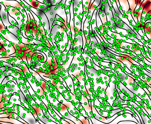
Figure 1.  $(a)$ The 3-D PTV set-up.
  $(b)$ PTV particles (green) superimposed onto an instantaneous snapshot of vorticity
  $\omega _z$ (red/black) and local streamlines (continuous lines). Note that PIV and PTV were performed in separate experiments and that the present picture illustrates the density of particles with respect to the scales of flow features. In addition, particles are accumulated in the
  $z$ direction, which gives an impression of high density. However, experiments are performed in the dilute regime and the solid fraction is of the order of
  $10^{-5}$. In the present study, PIV is used to compute flow quantities such as isotropy and dissipation while PTV is used to compute particle relative velocity variance, radial distribution functions and conditional concentration kernels. In panel
  $(b)$, particles were made larger than their real counterpart to appear visible and highlight the volume of measurement of the PTV.
  $(c)$ The 3-D trajectory samples in the volume shown in
  $(a)$ with particle tracks longer than
  $250$ frames. Measurements in both panels
  $(b)$ and
  $(c)$ were performed for the flow condition III (see table 1).
In the PIV system, the light source is a Nano L 135-15 pulsed Nd:YAG laser from Litron Lasers, outputting a light beam at 532 nm, and generating a vertical laser sheet through the centre of the tank. LaVision Glass Hollow Spheres 110P8 (density  $1.10\pm 0.05\ {\rm g}\ {\rm cm}^{-3}$, and mean size
  $9\unicode{x2013}13\ \mathrm {\mu }{\rm m}$) were used as seeding particles. The instantaneous PIV images were captured by an IMPERX B3320-8MP charge-coupled device (CCD) camera (
 $3312\ \text {pixel}\times 2488\ \text {pixel}$) equipped with a Nikon Nikkor-O Auto 35 mm
  $f/2$ lens. The camera was synchronised with the laser at a frame rate of
  $1$ Hz with a delay of 0.25 ms between two successive frames. Synchronisation with the laser was performed using a DG535 pulse generator. The software Stream Pix 7 was used for data stream acquisition. The image pairs were processed with DPIVSoft-2010 (Meunier & Leweke Reference Meunier and Leweke2003; Passaggia, Leweke & Ehrenstein Reference Passaggia, Leweke and Ehrenstein2012; Passaggia et al. Reference Passaggia, Chalamalla, Hurley, Scotti and Santilli2020) by means of interrogation windows with dimensions
  $64\ \text {pixel}\times 64 \text {pixel}$ for the first pass and
  $32\ \text {pixel}\times 32\ \text {pixel}$ for the second pass with 50 % overlap. The spatial resolution is approximately
  $43.4\ \mathrm {\mu }{\rm m}\ {\rm pixel}^{-1}$. The dimensions of the field of view are
  $14.4\ \text {cm}\times 10.8\ \text {cm}$. Three different turbulent intensities were generated by varying the frequency
  $(f)$ of the imposed oscillations (
 $1$ Hz,
  $1.5$ Hz and
  $2.5$ Hz) with a fixed oscillating stroke of
  $4$ cm, while statistics were obtained by averaging over
  $750$ realisations. The isotropy ratio
  ${u_{1,rms}}/{u_{2,rms}}$ measured using PIV provided values between
  $0.8$ and
  $1.3$, indicating a good degree of isotropy for the three flow conditions. The normalised root-mean-square (r.m.s.) velocities (Hwang & Eaton Reference Hwang and Eaton2004) are
  ${u_{1,rms}}/{\overline {u_{1,rms}}}\approx 0.9\unicode{x2013}1.2$ and
  ${u_{2,rms}}/{\overline {u_{2,rms}}\approx 0.8\unicode{x2013}1.3}$. Although the velocity field in the vertical direction is slowly decaying, it still can be seen as nearly homogeneous in the region of interest. The turbulent kinetic energy dissipation rate (
 $\epsilon$) was estimated by means of a time-averaged turbulent kinetic energy budget from the PIV data, detailed in Appendix A (see table 1 for the computed values).
Table 1. Driving parameters and turbulent flow characteristics.

The turbulent spectrum was then computed from the PIV data, and the compensated horizontal energy spectrum  $E_{11}k^{5/3}\epsilon ^{-2/3}$ is shown in figure 2(a) for the three flow conditions. The compensated spectra are essentially flat, confirming the existence of an inertial range for all flow conditions. The horizontal axis is normalised with the Taylor microscale (
 $\lambda$) computed as
  $\lambda = \sqrt {10\nu k/\epsilon }$, where
  $k$ is the mean turbulent kinetic energy estimated as
  $k=3(u'_{rms}+v'_{rms})/4$ and
  $\nu$ is the kinematic viscosity of water. The turbulence Reynolds number is
  $Re_{\lambda } = u'(\lambda /\nu )$, where
  $u'=\sqrt {2k/3}$ is the r.m.s. of the velocity fluctuations and provides values
  $Re_{\lambda }=[120,150,202]$ for the three oscillating frequencies. Note that the lowest value of
  $Re_{\lambda }$ is relatively close to that from the DNS of Ten Cate et al. (Reference Ten Cate, Derksen, Portela and Van Den Akker2004) with similar particles.

Figure 2.  $(a)$ Normalised horizontal velocity spectra from PIV measurements, where
  $k_\lambda = 2{\rm \pi} /\lambda$ is the Taylor microscale wavenumber.
  $(b)$ Autocorrelation function
  $h_{1,1}(x/M)$ for the three different flow cases.
In addition, the horizontal autocorrelation function of velocity fluctuations  $h_{1,1}(x/M)$ was calculated in order to estimate the horizontal integral length scale
  $\mathcal {L}_{11}$ and is reported in figure 2(b). This
  $\mathcal {L}_{11}$ was calculated from the zero crossing of
  $h_{1,1}(x/M)$ and slowly increases with the oscillating frequency as reported in table 1. The Kolmogorov equilibrium number
  $C_\epsilon = \epsilon \mathcal {L}_{11}/u'^{3}\approx 1$ was found to be nearly constant and close to the mean value observed in the compensated spectra reported in figure 2(a). Note that, in our experiments,
  $C_\epsilon \approx 1$ is close to the canonical value of
  $0.9$ (Vassilicos Reference Vassilicos2015). For the lower value of
  $Re_\lambda$, a residual large-scale circulation exists but its amplitude with respect to turbulence kinetic energy decreases with increasing stroke frequency
  $f$. This mean flow is composed of large-scale circulation regions whose amplitude is stronger in the bottom and decreases closer towards the grid. In the region where PTV measurements are performed, the mean velocity
  $\sqrt {K}$ (where
  $K$ is the mean flow kinetic energy) is roughly half the r.m.s. of the turbulent kinetic energy in this region. The resulting ratio between the mean-field kinetic energy and the turbulent kinetic energy is
  $0.27$ for the worst-case scenario when
  $f=1\ {\rm Hz}$ and decreases to
  $0.19$ for
  $f=2.5$ Hz.
A schematic of the 3-D PTV and planar two-component PIV set-up is shown in figure 1(a). The 3-D PTV imaging system consists of four synchronised Grasshopper3  $3.2$ MP cameras. A continuous-wave argon ion laser was used to generate a cylindrical laser volume of
  $4$ cm diameter through the tank. During PTV experiments, the tank was first filled with pre-filtered saline solution. The calibration process was then conducted to determine the interior and exterior parameters of the cameras, the lens distortions and electronic effects (Maas et al. Reference Maas, Gruen and Papantoniou1993). To quantify uncertainty in the calibration process, the real positions of points on the calibration block were compared with the positions measured from PTV (Akutina Reference Akutina2016), and the r.m.s. of the errors obtained were
  ${\rm r.m.s.}_x=0.0203\ {\rm mm}$,
  ${\rm {r.m.s.}}_y=0.0244 {\rm mm}$ and
  ${\rm r.m.s.}_z=0.0240\ {\rm mm}$. Quasi-monodisperse polyethylene microspheres (Cospheric LLC) with density
  $\rho _p=1.084\ {\rm g}\ {\rm cm}^{-3}$ (the same as the density of saline solution
  $\rho _f$) and diameter range
  $D=106\unicode{x2013}125\ \mathrm {\mu }{\rm m}$ were used for PTV and, for each flow condition,
  $0.15$ mg of particles were used consisting in a dilute volume fraction
  $O(10^{-5})$. The particle Stokes number,
  $St\equiv {\tau _p/\tau _\eta }$, the ratio of the particle response time
  $\tau _p=\rho _p D^{2}/18\mu _f$ (where
  $\mu _f$ is the fluid dynamic viscosity) to the turbulent Kolmogorov time scale
  $\tau _\eta =\sqrt {\nu /\epsilon }$, ranges from
  $St=0.0028$ to
  $St=0.0080$ in the three flow conditions. The particles were allowed to mix for one minute after being dispersed, before data acquisition began. A series of 72 000 images (
 $10$ min at
  $120\ {\rm frames}\ {\rm s}^{-1}$) per camera were then captured. On average, the number of voxels moved per frame with an acquisition rate at
  $120$ Hz is of the order unity for flow condition I, two voxels for flow condition II, and three voxels for flow condition III, which is the size of an individual particle for the latter (see table 1).
The 3-D PTV data processing performed in OpenPTV can be divided into two major parts: determination of particle positions in spatial coordinates and tracking of individual particles through consecutive images. The approach of Willneff (Reference Willneff2003) is used in the present study and combines the two steps together with a spatio-temporal matching method which improves tracking efficiency of particles by 10–30 % (Lüthi, Tsinober & Kinzelbach Reference Lüthi, Tsinober and Kinzelbach2005). Willneff's method predicts particle motion based on particle tracking in image and object space to resolve ambiguous particle image positions and correspondences. In other words, ‘temporal’ information at time  $t$ is used to resolve ‘spatial’ uncertainties regarding the existence and positions of particles in the next time step
  $t + \Delta t$. The seemingly modest improvement of 10–30 % in tracking efficiency is very significant in the context of further processing and analysis. Particle trajectories that are longer than the relevant Kolmogorov scales,
  $\eta$ and
  $\tau _\eta$, are the key prerequisite for a Lagrangian flow analysis, and they also significantly enhance the accuracy of the applied processing to obtain velocity derivatives (Lüthi et al. Reference Lüthi, Tsinober and Kinzelbach2005). To track particles, i.e. to find corresponding particles in image and object space of consecutive time steps, three criteria are used for effective assignment. First, a 3-D search volume is defined by minimum and maximum velocities in all three coordinate directions. Second, the Lagrangian acceleration of a particle is limited, defining a conic search area. Third, in the case of ambiguities, the particle leading to the smallest Lagrangian acceleration is chosen. Similarities in brightness, width, height and sum of grey values of the pixel of a particle image in two consecutive time steps proved to be not as valuable as expected. From the
  $565$ detected particles per frame for which a position in space can be determined, typically
  $470$ particles can be followed long enough, which is equivalent to a tracking efficiency of
  ${\sim }80$ % and a seeding density for linked particles of
  ${\sim }26$ particles cm
 $^{-3}$.
An instantaneous vorticity  $\omega _z$ and some 3-D trajectory samples at
  $f=2.5$ Hz (i.e. flow condition III) are shown in figures 1
 $(b)$ and 1
 $(c)$, respectively. Figure 1
 $(b)$ illustrates the particle density accumulated in the out-of-plane direction as well as the size of the relevant scales in the experiment. Note that both results were acquired in separate experiments.
2.2. Conditional concentration kernel models
The collision rate between particles in a monodisperse system can be described as (Wang et al. Reference Wang, Wexler and Zhou1998)
 \begin{equation} \mathcal{N}_c=\varGamma^{d}\frac{\bar{n}^{2}}{2}, \end{equation}
where  $\mathcal {N}_c$ is the collision rate per unit volume and
  $\bar {n}$ is the particle number concentration, defined as
  $N_p/\varOmega$, where
  $N_p$ is the number of particles and
  $\varOmega$ is the observation volume. The dynamic kernel
  $\varGamma ^{d}$, namely the ratio of concentration rate conditioned based on the distance
  $d$ to particle pair concentration (Rosa et al. Reference Rosa, Parishani, Ayala, Grabowski and Wang2013), can be obtained by directly measuring
  $N_p$,
  $\varOmega$ and the number of events when particles are separated by a certain distance
  $d$ over time. The conditional concentration is obtained by counting the number of particles located at a distance smaller than or equal to a given inter-particle distance
  $d > D$, which is then averaged in time. In what follows, we report conditional concentrations down to
  $d/D=2$. The associated error level is dependent only on the number of events measured during the experiment and is below 5 % for all cases considered in the present study.
In the pioneering work of Saffman & Turner (Reference Saffman and Turner1956), the conditional concentration kernel was described as the average volume of fluid entering a sphere per unit time. Saffman & Turner showed that this kernel for zero-inertia particles can be written as
 \begin{equation} \varGamma(d)=2{\rm \pi}{d^{2}}\langle |w_r(d)|\rangle, \end{equation}
where  $d \geqslant D$ is the distance between two particles. The particle pair radial relative velocity
  $w_r(d)$ at a separation distance
  $d$ is defined as
  $w_r(d) = (\boldsymbol {v}_2-\boldsymbol {v}_1)\boldsymbol {\cdot } \boldsymbol {d}/|\boldsymbol {d}|$ (Dou et al. Reference Dou, Ireland, Bragg, Liang, Collins and Meng2018b). The subscript
  $r$ means ‘radial’ and, since the velocity component perpendicular to the separation vector is not relevant to the particle conditional concentration nor collision, we will refer to radial relative velocity as ‘relative velocity’ from here on. Here
  $\boldsymbol {v}_2$ and
  $\boldsymbol {v}_1$ are the velocities of particles 1 and 2,
  $\boldsymbol {d}/|\boldsymbol {d}|$ denotes the unit vector in the direction parallel to the separation vector, and
  $\langle \cdot \rangle$ denotes the ensemble average. Further assuming that
  $d\ll \eta$, uniform particle concentrations in space and probability distributions of the velocity gradient being Gaussian, Saffman & Turner (Reference Saffman and Turner1956) proposed the following expression for the conditional concentration kernel in turbulent flows:
 \begin{equation} \varGamma^{ST}(d)=1.294{d^{3}}\left(\frac{\epsilon}{\nu}\right)^{1/2}. \end{equation}
Note that this concentration kernel reduces to the collision kernel when  $d=D$, that is, when the separation distance is equal to one diameter.
The theoretical description of  $\varGamma (d)$, (2.2), was then further developed by Sundaram & Collins (Reference Sundaram and Collins1997) to take into account non-uniform particle spatial distribution:
 \begin{equation} \varGamma^{K}(d)=4{\rm \pi}{d^{2}}g(d)\langle w_r(d)^{-}\rangle, \end{equation}
where  $g(d)$ is the RDF, which serves as a correction to the particle number concentration due to non-uniform particle distribution. Here,
  $\langle w_r(d)^{-}\rangle$ represents the inward particle radial relative velocity, which relates to particle pairs moving towards one another. The inward radial relative velocity can be further expressed as (Sundaram & Collins Reference Sundaram and Collins1996)
 \begin{equation} \langle w_r(d)^{-}\rangle=\int_{-\infty}^{0} -w_rP(w_r \mid d)\,{\rm d}w_r, \end{equation}
where  $P(w_r \mid d)$ is the p.d.f. of
  $w_r$ conditioned on the inter-particle distance
  $d$. The kinematic conditional concentration kernel
  $\varGamma ^{K}$, (2.4), thus combines the effects of the particles’ relative motion and particles’ preferential concentration.
2.3. Conditional concentration kernel measurements
In order to determine dynamic conditional concentration kernels for small separation distances, the present study considers the method introduced in Balachandar (Reference Balachandar1988) and Wang et al. (Reference Wang, Wexler and Zhou1998) to detect inter-particle distances. The analysis mainly focuses on geometric particle overlap for a given separation distance.
Inter-particle distance corresponding to collisions (i.e. when  $d=D$) is particularly challenging in laboratory experiments. The time scale associated with physical collisions of real particles (i.e.
  $D\approx 0.116$ mm in the present study) is much smaller than the temporal resolution of the experimental set-up (Yang & Hunt Reference Yang and Hunt2006; Monchaux et al. Reference Monchaux, Bourgoin and Cartellier2010; Marshall Reference Marshall2011; Ababaei et al. Reference Ababaei, Rosa, Pozorski and Wang2021). Instead, we consider analogous particles (Hill, Nowell & Jumars Reference Hill, Nowell and Jumars1992), which are fluid volumes centred on real particles with effective diameters larger than
  $D$. The conditional concentration detection was thus based on the effective particle diameters
  $d$ (which are adjustable) to obtain a relationship between conditional concentration kernels and thereby analogous collision kernels versus effective particle diameter. A schematic of effective diameters is shown in figure 3(a). Care should be taken to ensure that the effective diameters are small enough that the analogous particles can still be seen as inertialess and follow the fluid (and their host particles’) motion faithfully. The conditional concentration kernel derived using the ‘ghost events’ approximation will be denoted as
  $\varGamma ^{d}_{gh}$. This method counts all possible inter-particle distances below a given threshold but does not take into account the nature of the particles’ relative motion. A more realistic scheme is also considered: in the case of a particle pair candidate, if there are multiple points along the trajectories when two particles approach one another with distances smaller than their effective diameter (i.e. a multiple conditional concentration event), only the first instance meeting the threshold is considered. This conditional concentration kernel is denoted as
  $\varGamma ^{d}_{re}$.

Figure 3.  $(a)$ Sketch of the particle coordinate system, distances and angles used in the analysis. Analogous particle conditional concentration events are shown with dashed lines.
  $(b)$ Time-averaged RDF measured under three flow conditions. The distance is normalised by the particle diameter.
  $(c)$ Sketch of the measurement method of the radial distribution function. Particles in grey are in the range
  $d=[0.98r, 1.02r]$ from the red particle, while the blue particles are out of that range.
  $(d)$ P.d.f.s of particle pair radial relative velocity conditioned on different separation distances at 2.5 Hz. The particle relative velocities are normalised by the Kolmogorov velocity scale
  $u_\eta$. The p.d.f. of the standard normal distribution is also given for comparison.
For the kinematic conditional concentration kernel, the RDF is calculated by the following expression (McQuarrie Reference McQuarrie1976; de Jong et al. Reference de Jong, Salazar, Woodward, Collins and Meng2010):
 \begin{equation} g(r_i)=\frac{N_i/\Delta V_i}{N/V}. \end{equation}
At each time step of the experiment, an arbitrary particle's location is taken to be at the origin  $O$. In the above,
  $N_i$ is the number of particles that lie within a range of
  $[0.98r_i, 1.02r_i]$ relative to this origin (a spherical shell),
  $r_i$ is the average radius of the spherical shell,
  $\Delta V_i$ is the volume of the spherical shell,
  $i$ is the discrete index, and
  $N/V$ is the average particle number concentration. The RDF
  $g(r_i)$ is averaged over all the cases in which each particle takes a turn to serve as the origin and then averaged again over time. A sketch of the way the RDF is calculated is shown in figure 3(c). Periodic boundary conditions are used to cope with the reduction of the number of particles at larger particle separation distances (de Jong et al. Reference de Jong, Salazar, Woodward, Collins and Meng2010).
Figure 3(b) shows the time-averaged RDF measured for the three flow conditions with separations from less than the Kolmogorov length scale to the integral length scale. In the case of inertialess particles in turbulence, there is no preferential concentration and the RDF should equal unity. However, when the particle separation  $d/D<5$, the RDF is smaller than
  $0.8$ (see figure 3b). This result can seem surprising at first, since most studies analysed inertial particles, which tend to collide. For inertialess particles, the picture is somewhat different, since hydrodynamic effects can prevent particles coming near contact and can span large inter-particle distances because of the viscous nature of the flow. The recent DNS of inertial particles in homogeneous turbulence by Ababaei et al. (Reference Ababaei, Rosa, Pozorski and Wang2021) shows that the RDF can drop well below unity when
  $r/D<3.5$,
  $St_k<0.1$, and when long-range many-body interactions and lubrication forces are taken into account. Thus, it is essential to take
  $g(r)$ into account when measuring conditional concentration kernels when the separation distance is small, even for inertialess particles. The particle radial relative velocities were collected and binned according to the particle separation distance
  $r$ with a bin size in the range
  $[0.98r,1.02r]$. Ranges
  $[0.95r,1.05r]$ and
  $[0.9r,1.1r]$ were also tested, but without noticeable differences on the RDF. Then
  $\langle w_r(d)^{-}\rangle$ was calculated according to (2.5).
2.4. Fluid and particle radial relative velocity
Hereafter, we evaluate the following: (i) the dynamic conditional concentration kernel  $\varGamma ^{d}$ by directly measuring the number of particles for separation distances lower than
  $d$, the volume these particles occupy and the number of events; (ii) the kinematic conditional concentration kernel
  $\varGamma ^{K}$ through (2.4) by measuring
  $\langle w_r(d)^{-}\rangle$ and the RDF at different effective diameters; and (iii) the Saffman & Turner (Reference Saffman and Turner1956) concentration kernel
  $\varGamma ^{ST}$ through (2.3) by measuring the turbulent energy dissipation rate
  $\epsilon$, and we provide a comparison. (iv) We also use the second-order relative velocity structure functions of particles
  $S^{P}_{2\parallel } \equiv \langle w_r(r)^{2}\rangle$, following the nomenclature in Bragg & Collins (Reference Bragg and Collins2014b) and assuming that particles strictly follow fluid particles.
We use the second-order relative velocity structure functions for the fluid  $S^{f}_{2\parallel }$ as a reference to deduce the scaling laws of particle motions and determine the behaviour of
  $S^{P}_{2\parallel }$. According to Kolmogorov theory, the second-order relative velocity structure function is given by
 \begin{equation} S^{f}_{2\parallel} = \left\{\begin{array}{@{}ll} \dfrac{\epsilon}{15\nu}r^{2}, & {\rm{for}}\ \eta< r<\lambda, \\[6pt] C_2(\epsilon r)^{2/3}, & {\rm{for}}\ \lambda\ll r\ll \mathcal{L}_{11}, \\ 2(u'^{2}), & {\rm{for}}\ r>\mathcal{L}_{11}, \end{array} \right. \end{equation}
where  $C_2$ is a constant,
  $u'^{2}$ is the mean turbulent velocity fluctuation squared and
  $\mathcal {L}_{11}$ is the integral length scale, measured using the autocorrelation method from the PIV and found to be nearly constant among the flow conditions at each location considered. In what follows, we show that, for small distances, finite-size effects can play an important role in determining the p.d.f. of particle relative velocity and their second-order structure function.
3. Results and discussion
In this section we analyse the statistical properties of relative particle motions across multiple scales, from the integral length scale characterising the mean size of the large eddies of turbulence down to below the Kolmogorov scale. We begin with the p.d.f.s of particle pair radial relative velocity conditioned on different separations for flow condition III in figure 3(d) and observe a remarkable deviation from the Gaussian distribution, particularly at small separation distances.
At large separation distances, the p.d.f.s of relative velocity are slightly negatively skewed, which is a natural consequence of vortex stretching in turbulence (Tavoularis, Bennett & Corrsin Reference Tavoularis, Bennett and Corrsin1978). For smaller separations (figure 3c), the p.d.f.s become symmetric, which is in line with the relative velocity p.d.f.s of Saw et al. (Reference Saw, Bewley, Bodenschatz, Ray and Bec2014), who did not observe significant skewness in their relative velocity p.d.f.s at  $r/\eta \approx 1$ for inertialess particles; the tails of our relative velocity p.d.f.s are somewhat higher but much lower than reported in Hammond & Meng (Reference Hammond and Meng2021) for inertial particles. The essentially straight tails for
  $r/D=3.5$ hint at a decrease of the particles’ relative motion, contrary to finite-Stokes-number particles where the tails of the p.d.f.s are wide. This further hints at the importance of particle–particle interactions for scales of the order of the particle size, and we analyse the motion of two finite-size inertialess particles using the structure function method together with asymptotic theory for the lubrication motion of two colliding particles.
3.1. Radial relative velocity variance and finite-size effects
The second-order particle relative velocity structure functions (i.e. particle relative velocity variance)  $S^{P}_{2\parallel }$ normalised by the square of Kolmogorov velocity scales
  $u^{2}_\eta$ are shown in figure 4(a). A feature of
  $r^{2/3}$ scaling in the inertial subrange is observed for
  $r>\lambda$, consistent with Kolmogorov theory in (2.7). The transitions between the viscous and the inertial subranges should scale as
  $r^{2}$ but exhibits a plateau in the range
  $\eta >r\gtrsim \lambda$ for flow conditions I and II. This is attributed to the effects of low Taylor Reynolds number and a loss of isotropy at these scales (see Kim & Antonia Reference Kim and Antonia1993) and the relatively small distance from the oscillating grid. For flow condition III, this region becomes slightly steeper and the plateau progressively disappears. Note that the same behaviour was observed in the particle-resolving DNS of Ten Cate et al. (Reference Ten Cate, Derksen, Portela and Van Den Akker2004) for similar Taylor Reynolds numbers and inertialess particles. As the radial distance approaches the integral length scale, the normalised particle relative velocity approaches a plateau defined by the energy-containing scale
  $\mathcal {L}_{11}$ given by the velocity structure function (2.7). However, due to the relatively short distance from the grid and the presence of the large-scale circulation, we obtain a prefactor close to
  $0.9$ instead of
  $2$ in this expression for the flow condition I. The prefactor increases to
  $1.4$ for the flow condition III.

Figure 4.  $(a)$ Normalised relative velocity variance from measurements for the particles
  $S^{P}_{2\parallel }$ (lines with symbols) acquired from PTV and the fluid
  $S^{f}_{2\parallel }$ (dashed lines) acquired from PIV in a separate experiment, with
  $u_\eta =(\nu \epsilon )^{1/4}$ being the Kolmogorov velocity scale.
  $(b)$ Normalised relative velocity variance
  $S^{P}_{2\parallel }$ from the DNS of Ten Cate et al. (Reference Ten Cate, Derksen, Portela and Van Den Akker2004) from their figure 10 but plotted in logarithmic scales exhibiting the same scaling laws as the present experimental study.
For  $r<\eta$, the relative velocity should abruptly drop to zero. However, the decay for
  $S^{P}_{2\parallel }$ is different from what was anticipated for
  $S^{f}_{2\parallel }$ and hints at particle–particle interaction. This can also be observed in figure 10 in Ten Cate et al. (Reference Ten Cate, Derksen, Portela and Van Den Akker2004) when plotted with logarithmic scales, which we report in our study for comparison and analysis (see figure 4b). A similar trend was also reported very recently in the DNS of Ababaei et al. (Reference Ababaei, Rosa, Pozorski and Wang2021) at high Taylor Reynolds numbers for inertial particles when long-range many-body interactions and lubrication effects were taken into account. Therefore, we analyse a new weaker scaling (see figure 4a) that accounts for the onset of combined effects of lubrication forces and finite-size effects since the motion of the fluid should not influence relative inward velocity for
  $r<\eta$.
In the low Reynolds-number regime for a spherical particle moving in a fluid, where the particle Reynolds number  $Re_p = u_\eta D/\nu \ll 1$, Mongruel et al. (Reference Mongruel, Lamriben, Yahiaoui and Feuillebois2010) proposed a model based on a second-order ordinary differential equation describing the temporal evolution of the particle–particle distance for two particles moving towards one another, assuming that lubrication is the dominant effect.
Starting from the equation of motion for a sphere approaching a fixed wall, or equivalently for two particles approaching head-to-back vertically (Marshall Reference Marshall2011), the equation of motion becomes
 \begin{equation} m_{p} \frac{\mathrm{d} V_{p}}{\mathrm{d} t}={-}6 {\rm \pi}R \mu V_{p}(\delta)\, f_{rr}(\delta, Re_p)+\frac{4}{3} {\rm \pi}R^{3}(\rho_{p}-\rho_f)g, \end{equation}
where  $\delta =(r-D)/D$ is the gap between two particles,
  $V_p$ is the particle velocity and
  $f_{rr}(\delta,Re_p)$ is the friction factor given in Cox & Brenner (Reference Cox and Brenner1967) as
 \begin{equation} f_{rr}(\delta, Re_p)= \frac{1}{\delta}+\frac{1}{5}\left[1+\frac{Re_p}{4}\right] \ln \left[\frac{1}{\delta}\right]+O(Re_p^{2}), \end{equation}
which diverges when  $r-D$ becomes asymptotically small or equivalently
  $\delta \rightarrow 0$. In the region very close to the wall, the velocity growth is modelled at first order by a linear growth with the normalised distance
  $\delta$ (in agreement with experiments (Mongruel et al. Reference Mongruel, Lamriben, Yahiaoui and Feuillebois2010; Marshall Reference Marshall2011)) of the form
 \begin{equation} V_p=\delta V_{St}^{m}, \end{equation}
where  $V_{St}^{m}$ is some characteristic velocity. Keeping only the terms on the right-hand side of (3.1) (i.e. neglecting particle inertia), it follows that in this region we take
 \begin{equation} f_{rr}(\delta, Re_p)=\frac{1}{\delta} \frac{V_{S t}}{V_{S t}^{m}}, \end{equation}
where  $V_{St}$ is the Stokes velocity which is chosen equal to
  $u_\eta =(\nu \epsilon )^{1/4}$, the Kolmogorov velocity scale. In the particular case
  $Re_p \ll 1$, then
  $f_{rr}(\delta, Re_p)= 1 / \delta$ and from the classical lubrication theory and
  $V_{S t}=V_{S t}^{m}$, it appears appropriate to use
  $V_{S t}^{m}$ as a velocity scale. We then define a dimensionless time
  $\tau =t V_{S t}^{m} / R$ then
  $V_{p} / V_{S t}^{m}=-\mathrm {d} \delta / \mathrm {d} \tau$. We further assume that the friction factor
  $f_{rr}$ can be used in the near-contact case (
 $\delta \ll 1$). Equation (3.1) is then rewritten in dimensionless form as
 \begin{equation} -St_{m} \frac{\mathrm{d}^{2} \delta}{\mathrm{d} \tau^{2}}=\frac{1}{\delta} \frac{\mathrm{d} \delta}{\mathrm{d} \tau}+1 , \end{equation}
where  $St_{m}=\rho _{p} (V_{St}^{m})^{2} /(\rho _{p}-\rho _{f}) g R$ is a modified Stokes number for the particle.
Izard, Bonometti & Lacaze (Reference Izard, Bonometti and Lacaze2014) then proposed a modified version of (3.5) where the effective roughness height  $\zeta _e$ for non-smooth spheres is included. In this case, the lubrication force
  $\boldsymbol {F}_{lub}$ between two finite-size particles (i.e. a particle
  $i$ and a particle
  $j$) of velocity
  $\boldsymbol {u}_{p i}$ and
  $\boldsymbol {u}_{p j}$ and radius
  $R_i$ and
  $R_j$, respectively, can be written as (Brenner Reference Brenner1961)
 \begin{equation} \boldsymbol{F}_{lub}={-}\frac{6 {\rm \pi}\mu (\boldsymbol{u}_{p i}\boldsymbol{\cdot} \boldsymbol{n}-\boldsymbol{u}_{p j} \boldsymbol{\cdot}\boldsymbol{n})} {r+\zeta_{e}}\left(\frac{R_{i}R_{j}}{R_{i}+R_{j}}\right)^{2} \boldsymbol{n}, \end{equation}
where  $\zeta _e$ accounts for the mean height of surface asperities of real particles. This allows for mimicking real particles and avoiding the divergence of the force in (3.5) when contact occurs (i.e.
  $r=D$). The present lubrication force becomes active only when the distance between particles
  $r$ is such as (
 $0\leqslant r \leqslant 2D$). This upper bound is in the range of the critical distance for which the velocity of the particle decreases due to the presence of the wall (see Izard et al. Reference Izard, Bonometti and Lacaze2014, and references therein). Using
  $\boldsymbol {F}_{lub}$ in (3.6) instead of
  $f_{rr}$ in (3.4), equation (3.5) becomes
 \begin{equation} St_{m}\frac{\mathrm{d}^{2} \delta}{\mathrm{d} \tau^{2}} + \frac{D}{\left(r-D+\zeta_{e}\right)} \frac{\mathrm{d} \delta}{\mathrm{d} \tau}+1 = 0. \end{equation}
Note that this equation remains valid for separation distances smaller than  $\eta =1\approx 3D$ (Izard et al. Reference Izard, Bonometti and Lacaze2014), even for small gap distances
  $r \gtrsim D$. In the present model, we obtained
  $St_m=[0.67, 0.98, 1.18]$,
  $\zeta _e/R=0.05$ and
  $R=5.5\times 10^{-5}$ m.
Equation (3.7) is integrated numerically and shown in figure 5(a) where the boundary conditions  $\delta (r/\eta =1)$ and
  $\mbox {d}\delta (r/\eta =1)/\mbox {d}\tau$ are set to the values obtained in figure 4(a). Figure 5(a) shows a similar behaviour to that reported in the experiment where the scaling for
  $\langle w_r(r)^{2} \rangle /u^{2}_{\eta }$ is less steep than originally predicted by the second-order structure function for distances smaller than the Kolmogorov length scale. In particular,
  $\langle w_r(r)^{2} \rangle /u^{2}_{\eta } \sim r/\eta$ for increasing forcing frequency
  $f$, which simultaneously corresponds to increasing the finite-size ratio
  $D/\eta$. In other words, the mean inward velocity variance
  $w_r(r)$ no longer evolves linearly with the radial distance
  $r$ but seems to follow a power law. From figure 4(a,b), the particle structure function
  $S^{P}_{2\parallel }$ appears to approach a scaling of the form
 \begin{equation} S^{P}_{2\parallel} \approx {r\epsilon/(15\nu)}, \quad \mbox{for}\ D\lesssim\eta \mbox{ and } r \leqslant \eta, \end{equation}
and could be due to lubrication effects, whose consequences perhaps persist at those large distances. A similar behaviour was also recently reported in Ababaei et al. (Reference Ababaei, Rosa, Pozorski and Wang2021) where lubrication effects and long-range many-body interactions were found to decrease the RDF and modify the relative velocity scaling for  $r/D<3.5$ at low but finite Stokes numbers.

Figure 5.  $(a)$ Normalised particle relative velocity variance from measurements for
  $S^{P}_{2\parallel }$ from the dynamic model (3.7) under three flow conditions.
  $(b)$ Sample trajectories showing two particles near contact measured for
  $f=2.5\ {\rm Hz}$ and
  $r/D=2$.
This scaling is compared to the numerical integration of (3.7) in figure 5(a) and provides a good agreement for all flow conditions. The comparison between measurements and the theoretical model for the inward velocity variance suggests that lubrication effects could be the physical mechanisms leading to the scaling  $\langle w_r(r)^{2}\rangle /u^{2}_{\eta }\sim r/\eta$. Next, we analyse the relative particle angles for separation distances
  $r\lesssim \eta$.
3.2. Relative angles at small separation distances
A characteristic sample of particle tracks is shown in figure 5(b) where the separation distance between the two particles is  $r/D=2$ for the flow condition III. It is interesting to see that both tracks follow one another before and after the smallest separation distance. This therefore leads to small relative velocity, in agreement with the interpretation of the p.d.f. shown in figure 3(d). The p.d.f. of different angles for small separation distances as a function of both the turbulent Reynolds number and the separation distance
  $r/D$ are analysed. Here we considered two different angles: the particle tangential velocity angle
  $\theta _\parallel$ and the particle relative position angle
  $\theta _\bot$ defined as
 \begin{equation} \cos(\theta_\parallel)=\frac{|\boldsymbol{v}_1\boldsymbol{\cdot}\boldsymbol{v}_2|} {|\boldsymbol{v}_1||\boldsymbol{v}_2|} \quad \mbox{and}\quad \cos(\theta_\bot)=\frac{|\boldsymbol{v}_1\boldsymbol{\cdot}\boldsymbol{r}|} {|\boldsymbol{v}_1||\boldsymbol{r}|}. \end{equation}
 We begin the analysis by representing the particles’ tangential velocity angle  $\theta _\parallel$ for different flow conditions in figure 6(a) and different separation distances
  $r/D$ in figure 6(c), before and after the smallest separation distance. For
  $r/D=2.5$, the peak of the p.d.f.s narrows as the forcing frequency is increased and the peak shifts from
  $\theta _\parallel \approx 22^{\circ }$ for the flow condition I to a nearly parallel angle
  $\theta _\parallel \approx 7^{\circ }$ for the flow condition III. It is interesting to note that, for
  $r/D=2.5$, the p.d.f. narrows for every flow condition before and after the smallest separation distance, which shows that hydrodynamic interactions modify the trajectories of the particles. In other words, after the smallest separation distance, the trajectories of the particles tend to align with one another and particles tend to fly along as depicted in figure 5.

Figure 6.  $(a)$ P.d.f. of particle tangential velocity angle
  $\theta _\parallel$, measured at
  $r/D=2.5$, and
  $(b)$ relative position angle
  $\theta _\bot$ as a function of the grid frequency.
  $(c)$ Same as panel
  $(a)$ but as a function of the separation distance
  $r/D$ before and after the smaller separation distance.
  $(d)$ Same as panel
  $(b)$ but as a function of
  $r/D$ measured for
  $f=2.5\ {\rm Hz}$.
The effect of the separation distance is shown in figure 6(c) before and after the smallest separation distance, for the flow condition III. While the p.d.f.s are self-similar for  $3 \leqslant r/D \leqslant 5$, the smaller separation distance (
 $r/D=2.5$) shows that particles tend to further align their trajectory.
The particle relative position angle  $\theta _\bot$ is reported for different flow conditions in figure 6(b) and different separation distances
  $r/D$ in figure 6(d), similar to figure 6(a,c). From both plots, it is clear that, near the smallest separation distance, at
  $r/D=2.5$, the p.d.f. peaks near
  $\theta _\bot \approx 85^{\circ }$ but the distributions flatten as the forcing frequency decreases. The peak also shifts from
  $\theta _\bot \approx 60^{\circ }$ for the flow condition I,
  $\theta _\bot \approx 68^{\circ }$ for the flow condition II and
  $\theta _\bot \approx 85^{\circ }$ for the largest forcing frequency. Similarly, figure 6(d) shows the effect of the separation distance
  $r/D$, where, for
  $r/D>3$, the p.d.f.s are essentially self-similar and peak at
  $\theta _\bot \approx 50^{\circ }$. These results are consistent with the DNS results of Wang et al. (Reference Wang, Franklin, Ayala and Grabowski2006), who analysed relative angles in homogeneous turbulent at low Taylor Reynolds numbers (i.e. up to 55). For
  $r/D\leqslant 3.5$ the angle tends to increase, which denotes that finite-size effects tend to modify the particle's relative position angle.
The analysis of the tangential velocity and relative position angles seems to confirm that particle pairs tend to follow one another for  $2.5\leqslant r/D\leqslant 5$, with a relative angle in the range
  $60^{\circ }\unicode{x2013}85^{\circ }$. Head-on or head-to-tail scenarios seem unlikely to occur. The fact that p.d.f.s are modified when
  $r/D\leqslant 3.5$ supports the idea that finite-size effects start to appear for small separation distances and prevent particles from colliding with one another. This is also in line with the fact that the RDF drops below one at small separation distances. Lubrication forces are likely to prevent particles from approaching one another, modifying their relative angle, and decrease the probability to observe particle pairs with small separation distances.
3.3. Conditional concentration kernels
Now that the dynamic conditional concentration kernel has been defined and that finite-size effects have been described, we continue with the analysis of the conditional concentration kernels by comparing direct measurements of the number of events where particles are observed at a given separation distance to the different available theories. In addition, finite-size effects will be found to play a key role in the normalised conditional concentration kernels for small separation distances, as already reported in the DNS of Ababaei et al. (Reference Ababaei, Rosa, Pozorski and Wang2021).
Conditional concentration kernels at small separation distances  $\varGamma ^{K}$,
  $\varGamma ^{d}_{gh}$,
  $\varGamma ^{d}_{re}$ and
  $\varGamma ^{ST}$ are compared in figure 7(a) with the averaged number of particles, observation volumes and particle number concentrations measured and reported in table 2. The observation volumes were measured with a QuickHull algorithm (Barber et al. Reference Barber, Dobkin, Dobkin and Huhdanpaa1996). In figure 7(a), only kernels for flow condition III are shown for clarity;
  $\varGamma ^{d}_{gh}$,
  $\varGamma ^{d}_{re}$ and
  $\varGamma ^{K}$ normalised by
  $\varGamma ^{ST}$ are shown in figure 7(b). We note the following.
(i) The ratio
${\varGamma ^{K}}/{\varGamma ^{ST}}$ decreases monotonically and falls below unity with decreasing separation distance. We attribute this deviation to finite-size effects. As mentioned above, the theory of Saffman & Turner (Reference Saffman and Turner1956) is based on the assumptions of negligible particle–particle interactions. In the present experiments, the particle separation distance becomes sufficiently small such that particle–particle interactions cannot be ignored. This effect starts to play a role for $r/D\leqslant 3.5$, as shown in figure 7. As the separation decreases and particles approach one another, finite-size effects act against particles’ collision, leading to a decrease in $\varGamma ^{K}$ compared with $\varGamma ^{ST}$.
Figure 7.
$(a)$ Measured conditional concentration kernels $\varGamma ^{K}$, $\varGamma ^{d}_{gh}$, $\varGamma ^{d}_{re}$ and $\varGamma ^{ST}$ for flow condition III and $(b)$ normalised conditional concentration kernels $\varGamma ^{K}$, $\varGamma ^{d}_{gh}$ and $\varGamma ^{d}_{re}$ by $\varGamma ^{ST}$ at the three flow conditions.AsTable 2. Measured particle number concentrations under the three flow conditions.
$r/D$ increases, finite-size effects become negligible and the ratio ${\varGamma ^{K}}/{\varGamma ^{ST}}$ becomes nearly constant. Saffman & Turner assumed that the probability distribution of the velocity gradient is Gaussian; however, the p.d.f. of particle pair radial relative velocity, shown in figure 3(d), is indeed not Gaussian at small distances. The finite ratio of particle size to Kolmogorov length scale leads to a larger particle relative velocity than that of fluid particles, which contributes to a larger $\varGamma ^{K}$.
(ii) The normalised conditional concentration kernels are found to be largely insensitive to the flow Reynolds number that we considered, which is consistent with Ireland, Bragg & Collins (Reference Ireland, Bragg and Collins2016).
(iii) We found
$\varGamma ^{D}_{gh}\approx (1.25\unicode{x2013}1.30)\varGamma ^{D}_{re}$ consistent with Voßkuhle, Pumir & Lévêque (Reference Voßkuhle, Pumir and Lévêque2011) (i.e. ghost events overestimate the real conditional concentration rate by ${\sim }30\,\%$ at small Stokes numbers).(iv) For
$r/D<3.5$, we observe that all concentration kernels increase with $r/D$, which is a consequence of the inward velocity modification for $r/\eta <1$ induced by finite-size effects, preventing particles from colliding.


4. Conclusion
Kinematic and dynamic conditional concentration kernels of solid inertialess particles in isotropic turbulence at low to intermediate Taylor Reynolds numbers with real particle diameters smaller than the Kolmogorov length scale are measured experimentally. Dynamic conditional concentration kernels are measured using 3-D PTV and fully resolved particles providing similar results with kinematic conditional concentration kernels. The high spatial resolution, large observation volume and long acquisition time allow for calculating particle relative velocity statistics over a wide range of distance  $r$ from the dissipation range to the integral scale range with
  $5\times 10^{5}$ particle relative velocity samples in each bin. This leads to over
  $10^{9}$ realisations, which allows for well-converged statistics. The particle relative velocity variance agrees well with Kolmogorov theory in the inertial subrange. For separation distances
  $r$ smaller than the Kolmogorov length scale
  $\eta$, finite-size effects lead to a new scaling of particle relative velocity variance compared to that of fluid particles where
  $S^{P}_{2\parallel } = {r\epsilon /(15\nu )}$ for particle diameters
  $D\lesssim \eta$ provides a good approximation. We speculate that the departure from point-tracer behaviour is due to long-range interactions together with lubrication forces, whose consequences perhaps persist at those large distances.
Both kinematic and dynamic conditional concentration kernels at small separation distances are compared with Saffman & Turner (Reference Saffman and Turner1956) theory. The deviation at small distance is attributed to finite-size effects (Ababaei et al. Reference Ababaei, Rosa, Pozorski and Wang2021), while, at larger distance, we recover the Saffman & Turner approximation. The present method allows for direct conditional concentration measurements, excluding multiple instances when the inter-particle distance falls below the distance  $d$ from the first (initial) instance for the calculation of the dynamic conditional concentration kernels. This is confirmed by
  $\varGamma ^{D}_{gh} \approx (1.25\unicode{x2013}1.35)\varGamma ^{D}_{re}$, close to the finding of Voßkuhle et al. (Reference Voßkuhle, Pumir and Lévêque2011), which demonstrated that the ‘ghost conditional concentration’ approach overestimates the conditional concentration kernel by up to
  $30\,\%$. Furthermore, normalised dynamic conditional concentration kernels appear to be independent of the present Reynolds number, in agreement with Ireland et al. (Reference Ireland, Bragg and Collins2016). Dynamic conditional concentration kernels are based on the measurement of inter-particle distances using analogous but larger particles centred on the real particles. Further experimental work, such as the recent study by Hammond & Meng (Reference Hammond and Meng2021), needs to focus on finite-size inertial particles, since analogous inertial particles would behave differently than real host particles near contact. Recent DNS by Ababaei et al. (Reference Ababaei, Rosa, Pozorski and Wang2021) show that finite-size effects should remain an important factor when inertial particles come into contact and largely contribute to accurately estimating collision kernels.
Acknowledgements
We would like to thank A.D. Bragg, A. Liberzon, D.L. Koch and S. Xu for helpful discussions. We acknowledge Longleaf Computing Cluster at the University of North Carolina at Chapel Hill and the support provided by the ITS Research Computing and the Joint Applied Mathematics and Marine Sciences Fluids Lab of UNC-Chapel Hill. We would also like to thank the reviewers for their useful and constructive comments.
Funding
The authors acknowledge the support of the National Science Foundation Grant Numbers OCE–1335088, OCE–1155558 and OCE–1736989.
Declaration of interests
The authors report no conflict of interest.
Appendix A. Estimation of the turbulent kinetic energy dissipation rate from PIV
Turbulence kinematic energy dissipation  $\epsilon$ could not be directly measured from the spectra reported in figure 2(a) because the PIV spectra hardly resolved the Taylor microscale
  $\lambda$, leaving most of the turbulence kinetic energy dissipation spectrum out of reach. Instead,
  $\epsilon$ was estimated based on the turbulence kinetic energy budget from 2-D PIV measurements. Here, we chose a rectangular control volume, located at the position of the laser volume used for PTV and shown in figure 1. Using the divergence theorem, the quantities are projected onto the surfaces of the control volume and the turbulence kinetic energy budget simplifies to
 \begin{equation} \int_{V} \epsilon\,{\rm d}V={-}\int_{S_x}(U \overline{k'}+\overline{u'k'})n_x\,\mbox{d}y -\int_{S_y}(V \overline{k'}+\overline{v'k'})n_y\,\mbox{d}x -\int_{V}^{} \overline{u_{i}^{\prime}u_{j}^{\prime}}U_{ij}\,\mbox{d}V, \end{equation}
where  $\epsilon$ is the local time-averaged turbulence kinetic energy dissipation,
  $S_x$ are the faces of the control volume in the horizontal direction
  $x$ while
  $S_y$ is oriented in the vertical direction
  $y$. Here, the overbar denotes the temporal mean,
  $(U,V)$ is the mean flow computed from all PIV snapshots and
  $\overline {k'}$ is the time-averaged turbulence kinetic energy. Note that the pressure–velocity diffusion term was neglected since it was not directly accessible from PIV measurements and because it plays no significant role in nearly homogeneous and isotropic turbulence (Sagaut & Cambon Reference Sagaut and Cambon2008). The spatially averaged turbulence kinetic energy dissipation rate
  $\epsilon$ was finally obtained by dividing the left-hand side of (A1) by the control volume
  $V$.
$V$.


