2. Governing equations, symmetries and numerics

Consider a fluid of kinematic viscosity $\nu$, thermal diffusivity $\kappa$ and coefficient of volume expansion $\beta$ contained in a cavity of square cross-section with sides of length $L$ and spanwise width $W$. The four sidewalls are thermally insulated, whereas the top and bottom endwalls are held at constant temperatures, with the temperature difference between the top and bottom walls ${\rm \Delta} T=T_{T}-T_{B}>0$. Gravity $g$ is aligned in the downward vertical direction. In the absence of any other external force, the fluid is linearly stratified and at rest. The system is non-dimensionalized using $L$ as the length scale and $1/N$ as the time scale, where $N=\sqrt {g\beta {\rm \Delta} T/L}$ is the buoyancy frequency. The non-dimensional temperature is $T=(T^*-T_{B})/{\rm \Delta} T - 0.5$. A Cartesian coordinate system fixed to the cavity is used with its origin at the centre of the cavity; $z$ is the vertical direction and $y$ is the spanwise direction, such that ${\boldsymbol {x}}=(x,y,z)\in [-0.5,0.5]\times [-W/2L,W/2L]\times [-0.5,0.5]$. The velocity is ${\boldsymbol {u}}=(u,v,w)$ and the vorticity is ${\boldsymbol {\omega }}= {\boldsymbol {\nabla }}\boldsymbol {\cdot }{\boldsymbol {u}}= (\omega _x,\omega _y,\omega _z)$. The cavity is subjected to harmonic oscillations in the vertical direction of angular frequency $f$ and vertical displacement $\ell$. Figure 1 is a schematic of the set-up.

Figure 1. Schematic of the vertically oscillating cavity. The perspective is of the clipped (boundary layers removed) spanwise vorticity $\omega _y$ for an $\textrm {L}_{1:0:1}$ response at ${\textit {Rn}}=2\times 10^{4}$, $\alpha _f=0.15$ and $\omega _f=1.41$.

Under the Boussinesq approximation, the non-dimensional governing equations in the cavity frame are

(2.1)\begin{equation} \left. \begin{array}{c@{}} {\partial {\boldsymbol{u}}}/{\partial t} + {\boldsymbol{u}}\boldsymbol{\cdot}\boldsymbol{{\nabla}}{\boldsymbol{u}} ={-}{\boldsymbol{\nabla}} p + {\textit{Rn}}^{{-}1}\nabla^2 {\boldsymbol{u}} + (1+\alpha_f\cos{\omega_f t})T {\boldsymbol{e}}_z, \quad {\boldsymbol{\nabla}}\boldsymbol{\cdot}{\boldsymbol{u}} = 0, \\ {\partial T}/{\partial t} + {\boldsymbol{u}}\boldsymbol{\cdot}{\boldsymbol{\nabla}} T = ({\textit{Pr}}\,{\textit{Rn}})^{{-}1}\nabla^2 T, \end{array}\right\} \end{equation}

where $p$ is the reduced pressure. There are five non-dimensional parameters:

(2.2)\begin{equation} \left.\begin{array}{cc@{}} \textrm{buoyancy number } & {\textit{Rn}} = NL^2/\nu, \\ \textrm{Prandtl number } & {\textit{Pr}} = \nu/\kappa, \\ \textrm{spanwise aspect ratio } & \gamma=W/L,\\ \textrm{forcing frequency } & \omega_f = f/N, \\ \textrm{forcing amplitude } & \alpha_f = f^2\ell/g. \end{array}\right\} \end{equation}

The no-slip boundary condition in the cavity frame is ${\boldsymbol {u}}=\textbf {{0}}$ on all six walls. The temperature boundary conditions are $T_x(\pm 0.5,y,z)=T_y(x,\pm 0.5\gamma ,z)=0$ and $T(x,y,\pm 0.5)=\pm 0.5$. The governing equations and boundary conditions are equivariant to reflections about the three midplanes, $\mathcal {K}_{x}$, $\mathcal {K}_{y}$ and $\mathcal {K}_{z}$. Their composition is a reflection through the origin, known as a centrosymmetry, whose action is

(2.3)\begin{equation} \mathcal{C}:[u,v,w,T](x,y,z,t) \mapsto [{-}u, -v, -w, -T]({-}x, -y, -z, t). \end{equation}

Owing to the periodic forcing, the system is also invariant to a time translation,

(2.4)\begin{equation} \mathcal{P}_\tau:[u,v,w,T](x,y,z,t) \mapsto [u,v,w,T](x,y,z,t+\tau), \end{equation}

where $\tau =2{\rm \pi} /\omega _f$ is the forcing period. The basic state,

(2.5a–c)\begin{equation} {\boldsymbol{u}}_b=\textbf{{0}},\quad T_b=z \quad\text{and}\quad p_b=0.5z^2(1+\alpha_f\cos{\omega_f t}), \end{equation}

is both $\mathcal {C}$ and $\mathcal {P}_\tau$ invariant. It exists for all values of the governing parameters, but loses stability as these are increased above critical levels. Instabilities are typically associated with symmetry breaking.

Linearizing (2.1) about the basic state (2.5a–c), neglecting thermal and viscous diffusion (taking ${\textit {Rn}}\to \infty$), and in the absence of gravitational modulations ($\alpha _f=0$), leads to an eigenvalue problem for the inviscid intrinsic modes of the stratified cavity. These modes are periodic in all three directions, satisfy no-penetration boundary conditions and can be obtained via separation of variables. They vary harmonically in time with frequency $\sigma _{m:k:n}\in (0,1)$, given in terms of integer half-wavenumbers $m$, $k$ and $n$ in the $x$, $y$ and $z$ directions by the dispersion relation

(2.6)\begin{equation} \sigma^2_{m:k:n}=\dfrac{m^2+(k/\gamma)^2}{m^2+(k/\gamma)^2+n^2}. \end{equation}

The spatial harmonics all have the same temporal frequency, $\sigma ^2_{m:k:n}=\sigma ^2_{jm:jk:jn}$ for any positive integer $j$. When $k=0$ or $\gamma \to \infty$, the modes reduce to the 2-D eigenmodes determined by Thorpe (Reference Thorpe1968), with $v=0$ and independent of $y$.

Space is discretized via spectral collocation with Chebyshev polynomials of degree $n_c$ in barycentric form, and time evolution uses the fractional-step improved projection scheme of Mercader, Batiste & Alonso (Reference Mercader, Batiste and Alonso2010). We have implemented this method previously in related problems (Lopez et al. Reference Lopez, Welfert, Wu and Yalim2017; Wu, Welfert & Lopez Reference Wu, Welfert and Lopez2018; Yalim et al. Reference Yalim, Lopez and Welfert2018, Reference Yalim, Welfert and Lopez2019b). Most of the results presented in this study were obtained with Chebyshev polynomials of degree $n_c=48$ in the $x$, $y$, and $z$ directions and up to 200 time steps per forcing period. Converged quasi-periodic flows were run for at least 50 000 forcing periods. Flows driven by large-amplitude forcing with wave breaking require much greater spatio-temporal resolution; for these cases $n_c=384$ and 4000 time steps per forcing period were used.

The flows are visualized using isotherms and spanwise vorticity contours at the spanwise midplane in order to allow for direct comparisons between 2-D and 3-D solutions, and

(2.7a,b)\begin{equation} Q_N =\frac{\|\boldsymbol{\mathsf{R}}\|^2-\|\boldsymbol{\mathsf{S}}\|^2}{\|\boldsymbol{\mathsf{R}}\|^2+\|\boldsymbol{\mathsf{S}}\|^2} = \frac{|{\boldsymbol{\omega}}|^2-\Phi}{|{\boldsymbol{\omega}}|^2+\Phi} , \quad Q_N\in[{-}1,1], \end{equation}

where $\boldsymbol{\mathsf{R}}=(\boldsymbol{\mathsf{J}}-\boldsymbol{\mathsf{J}}^{\,{\rm T}})/2$ is the rate-of-rotation tensor and $\boldsymbol{\mathsf{S}}=(\boldsymbol{\mathsf{J}}+\boldsymbol{\mathsf{J}}^{\,{\rm T}})/2$ is the rate-of-strain tensor, which are respectively the skew-symmetric and symmetric components of the velocity gradient tensor $\boldsymbol{\mathsf{J}}={\boldsymbol {\nabla }}{\boldsymbol {u}}$, $\Phi =2\|\boldsymbol{\mathsf{S}}\|^2$ is the viscous dissipation and $\|\cdot \|$ denotes the Frobenius norm. For incompressible flows, $Q_N=2Q/\|\boldsymbol{\mathsf{J}}\|^2$ is a normalization of the $Q$-criterion of Hunt, Wray & Moin (Reference Hunt, Wray and Moin1988), measuring the relative strengths of $\boldsymbol{\mathsf{R}}$ and $\boldsymbol{\mathsf{S}}$. On no-slip boundaries $Q_N=0$, and regions in space with $Q_N>0$ are where $\boldsymbol{\mathsf{R}}$ dominates over $\boldsymbol{\mathsf{S}}$. The isosurface level $Q_N=0.04$ (corresponding to level $(1+Q_N)/2=0.52$ of the related $\Omega$-criterion of Liu et al. (Reference Liu, Wang, Tang and Duan2016)) provides a remarkably good visualization of the flow's vortex structure in three dimensions.

3. Dynamics in the 1 : 0 : 1 subharmonic resonance tongue

Benielli & Sommeria (Reference Benielli and Sommeria1998) experimentally investigated the responses in a short spanwise cavity ($\gamma \approx 0.4$) at forcing frequency $\omega _f \approx 2/\sqrt {2}$, corresponding to the middle of the 1 : 0 : 1 subharmonic resonance tongue (the natural frequency of the 1 : 0 : 1 intrinsic mode is $\sigma _{1:0:1}=1/\sqrt {2}$). They had ${\textit {Rn}}\approx 1.2\times 10^{5}$ ($N={1.96}\ \textrm {s}^{-1}$, $L={25}\ \textrm {cm}$, $\nu ={0.01}\ \textrm {cm}^2\ \textrm {s}^{-1}$) and a Schmidt number of order 700 (corresponding to salt in water), which are quite challenging for an extensive numerical parametric study, even in two dimensions. In our 2-D numerical study (Yalim et al. Reference Yalim, Welfert and Lopez2019b), we used ${\textit {Rn}}=2\times 10^{4}$ and ${\textit {Pr}}=1$ for an extensive study in the forcing frequency and amplitude, considering $\omega _f\in (0,2.5)$ and $\alpha _f\in (0,1)$. In the present 3-D numerical study, we use the same geometry as Benielli & Sommeria (Reference Benielli and Sommeria1998), with $\gamma =0.4$, and also consider the response in the 1 : 0 : 1 subharmonic resonance tongue, with $\omega _f=1.41\approx 2/\sqrt {2}$ and $\alpha _f\in (0,0.3]$. We keep ${\textit {Rn}}={2\times 10^{4}}$ and ${\textit {Pr}}=1$ as in the 2-D study in order to make direct comparisons between the response flows in the two studies.

Figure 2 presents bifurcation diagrams from simulations in two dimensions (reproduced from Yalim et al. (Reference Yalim, Welfert and Lopez2019b)) and in three dimensions with $\gamma =0.4$, both at ${\textit {Rn}}=2\times 10^{4}$, ${\textit {Pr}}=1$ and $\omega _f=1.41$. The state measure in both is the variance in the $u$ velocity at a point, $\Sigma ^2_{2D}$ and $\Sigma ^2_{3D}$. The point in two dimensions is $(x,z)=(1/\sqrt {8},1/\sqrt {8})$ and in three dimensions it is at the corresponding point on the spanwise midplane $(x,y,z)=(1/\sqrt {8},0,1/\sqrt {8})$. The two bifurcation diagrams are qualitatively similar; the basic state (2.5a–c) loses stability to a limit cycle whose period is twice that of the forcing period; its spatial structure matches that of the 1 : 1 mode in two dimensions and the 1 : 0 : 1 mode in three dimensions, and the intrinsic frequencies of the modes are $\sigma _{1:1}=\sigma _{1:0:1}=1/\sqrt {2}\approx 0.5\omega _f$. The critical forcing amplitudes at onset of instability differ: $\alpha _f\approx 0.066$ in two dimensions versus $\alpha _f\approx 0.143$ in three dimensions. The larger forcing in three dimensions is needed to overcome the viscous damping from the spanwise walls at $y=\pm 0.5$. A snapshot of the spanwise vorticity $\omega _y$ at forcing phase ${\rm \pi} /2$ and the isotherms at forcing phase $3{\rm \pi} /2$ of the 2-D limit cycle $\textrm {L}_{1:1}$ and that of the 3-D limit cycle $\textrm {L}_{1:0:1}$ in the spanwise midplane $y=0$ are shown in the first column of figure 3. The states are a little beyond onset, at $\alpha _f=0.07$ for the 2-D and $\alpha _f=0.15$ for the 3-D cases. They are very similar. At the subharmonic bifurcation, both the centrosymmetry $\mathcal {C}$ and the $\tau$ periodicity $\mathcal {P}_\tau$ are broken; however, the cycles retain a spatio-temporal symmetry consisting of the composition $\mathcal {C}\mathcal {P}_\tau$ (a half-period-flip symmetry). Furthermore, $\mathcal {P}_\tau$ conjugates are also spawned, $\mathcal {P}_\tau (\textrm {L}_{1:1})$ in two dimensions and $\mathcal {P}_\tau (\textrm {L}_{1:0:1})$ in three dimensions. All have invariance to the combined reflections in $x$ and $z$, $\mathcal {K}_{x} \mathcal {K}_{z}$ (but not to just one or the other reflection), and L$_{1:0:1}$ is also spanwise reflection $\mathcal {K}_{y}$ invariant.

Figure 2. Bifurcation diagrams at ${\textit {Rn}}=2\times 10^{4}$, ${\textit {Pr}}=1$ and $\omega _f=1.41$ for $(a)$ the 2-D study and $(b)$ the 3-D study with $\gamma =0.4$. In both panels, the primary subharmonic limit cycles are denoted in red, the symmetric-conjugate limit cycles in blue, quasi-periodic states of two or three frequencies in yellow, and a myriad of complex states, including chaos, in green.

Figure 3. Snapshots of subharmonic limit cycle response flows for ${\textit {Rn}}={2\times 10^{4}}$, ${\textit {Pr}}=1$ and forcing frequency $\omega _f=1.41$ at forcing amplitude $\alpha _f$ as indicated: (a) spanwise vorticity $\omega _y$ and isotherms of 2-D flows from Yalim et al. (Reference Yalim, Welfert and Lopez2019b); (b) $\omega _y$ and the isotherms of 3-D flows in the spanwise midplane $y=0$, but at different $\alpha _f$ as indicated. The isotherms and $\omega _y$ are shown a half-forcing-period apart.

The limit cycles undergo a pitchfork bifurcation, at $\alpha _f\approx 0.101$ in two dimensions and $\alpha _f\approx 0.167$ in three dimensions, breaking the half-period-flip symmetry $\mathcal {C}\mathcal {P}_\tau$ and spawning two subharmonic limit cycles, $\textrm {LL}_{2D}$ and $\textrm {LR}_{2D}$ in two dimensions and $\textrm {LL}_{3D}$ and LR$_{3D}$ in three dimensions (along with their $\mathcal {P}_\tau$ conjugates). These states are symmetrically related by a reflection either in $x$ or in $z$: $\mathcal {K}_{x}\,\textrm {LL} = \textrm {LR}$ and $\mathcal {K}_{z}\,\textrm {LL} = \textrm {LR}$, in both two and three dimensions. The second and third columns of figure 3 show snapshots of these. The fourth column of figure 3 shows snapshots of another limit cycle, $\textrm {L}_{2:2}$ in two dimensions and $\textrm {L}_{2:0:2}$ in three dimensions; these are spatial harmonics of $\textrm {L}_{1:1}$ and $\textrm {L}_{1:0:1}$. They are unstable in the full space, but stable in the $\mathcal {C}$-invariant subspace in which they were computed. All these limit cycles have the same frequency, $0.5\omega _f$.

Figure 4 shows a 3-D perspective of the same 3-D states from figure 3 (supplementary movie 1, available at https://doi.org/10.1017/jfm.2020.543, animates the four limit cycles over two forcing periods). The temperature deviation is maximal a half-forcing-period (a quarter period of the subharmonic response) after the maximal response in the spanwise vorticity. When the magnitude of vorticity (which is pointing almost entirely in the spanwise direction) is small in the interior, the $Q_N=0.04$ isosurface retracts to the boundary layer regions where dissipative effects dominate.

Figure 4. Snapshots of subharmonic limit cycle response flows for ${\textit {Rn}}=2\times 10^{4}$, ${\textit {Pr}}=1$ and forcing frequency $\omega _f=1.41$ at forcing amplitude $\alpha _f$ as indicated. The spanwise vorticity $\omega _y$ and the normalized $Q$-criterion $Q_N$ are shown a half-forcing-period behind the isotherms $T$. The $T$ value is used to colour the $Q_N=0.04$ isosurface. Supplementary movie 1 provides an animation over two forcing periods.

So far, we have found direct, albeit qualitative, correspondence between the response flows in two and three dimensions. Further increasing $\alpha _f$ beyond $\alpha _f\approx 0.110$ in two dimensions and $\alpha _f\approx 0.193$ in three dimensions, LL and LR (and their conjugates $\mathcal {P}_\tau \textrm {LL}$ and $\mathcal {P}_\tau \textrm {LR}$) lose stability via a Neimark–Sacker bifurcation. Following the Neimark–Sacker bifurcation, a pair of symmetrically related quasi-periodic solutions $\textrm {QL}_{3D}$ and $\textrm {QR}_{3D}$ (along with their $\mathcal {P}_\tau$ conjugates) are spawned. These quasi-periodic solutions are characterized by two frequencies and exist on 2-tori in phase space. The first frequency is inherited from the progenitor subharmonic limit cycles ($\textrm {LL}_{3D}$ and $\textrm {LR}_{3D}$), while the second frequency is lower and corresponds to slow drifts to and from the $\textrm {L}_{2:0:2}$ saddle limit cycle. Supplementary movie 2 shows an animation of the $Q_N$-criterion at isolevel $Q_N=0.04$ of $\textrm {QR}_{3D}$ at $\alpha =0.234$ strobed every two forcing periods at forcing phase ${\rm \pi}$ over 176 forcing periods. This movie illustrates the slow drift in the $\textrm {QR}_{3D}$ heteroclinic dynamics between the saddle states $\textrm {L}_{1:0:1}$, $\textrm {LR}_{3D}$ and $\textrm {L}_{2:0:2}$.

Increasing $\alpha _f$ beyond 0.234, $\textrm {QL}_{3D}$ and $\textrm {QR}_{3D}$ (along with their $\mathcal {P}_\tau$ conjugates) undergo a period-doubling cascade. Strobing the phase portrait of the flow every two forcing periods, the period doubling is illustrated for several $\alpha _f$ in figure 5. The last computed $\textrm {QR}_{3D}$ prior to period doubling is illustrated at $\alpha _f=0.234$; the strobed phase portrait is a single-loop cycle corresponding to the low frequency in the quasi-periodic $\textrm {QR}_{3D}$. Quasi-statically increasing the forcing amplitude to $\alpha _f=0.235$, the low frequency is observed to halve (period double) as the strobe map now consists of a two-loop cycle. The period-doubling sequence continues: by $\alpha _f=0.238$ the strobe map cycle has four loops and 16 loops at $\alpha _f=0.239$. Increasing $\alpha _f$ further reveals the classic period-doubling route to chaos, culminating at $\alpha _f\approx 0.247$ where the $\mathcal {K}_{x}\mathcal {K}_{z}$ symmetry is broken. The spanwise $\mathcal {K}_{y}$ symmetry is preserved throughout this cascade.

Figure 5. Strobe maps (every two forcing periods at forcing phase 0) of $\textrm {QR}_{3D}$ using the kinetic energy $E_k=0.5\iiint _V {\boldsymbol {u}}^2\, \textrm {d}V$ and global temperature measure $E_T=30\iiint _V T^2\, \textrm {d}V$ at $\omega _f=1.41$ and $\alpha _f$ as indicated. Supplementary movie 2 animates the $\alpha _f=0.234$ case.

The symmetry-broken $\textrm {QL}_{3D}$ and $\textrm {QR}_{3D}$ states at $\alpha _f\approx 0.247$ undergo intermittent drifts to and from the $\mathcal {K}_{x}\mathcal {K}_{z}$-symmetry subspace. On increasing $\alpha _f$, the drifts away from the $\mathcal {K}_{x}\mathcal {K}_{z}$-symmetry subspace increase in intensity and duration, resulting in the flow momentarily visiting a sloshing state whose dynamics are reminiscent of the dynamics of the 3-tori observed in the 2-D case (Yalim et al. Reference Yalim, Welfert and Lopez2019b).

One of the main findings in Yalim et al. (Reference Yalim, Welfert and Lopez2019b) was the unravelling of the gluing bifurcations of the 2-D left- and right-handed quasi-periodic flows into a single symmetric quasi-periodic flow. Such dynamics are also observed here in three dimensions for $\alpha _f\ge 0.247$. An example of a glued solution at $\alpha _f=0.26$ is shown in figure 6, which includes a strobed (every two forcing periods) phase portrait of the flow along with a selection of flow snapshots. This glued state is $\mathcal {K}_{x}\mathcal {K}_{z}$ symmetric and experiences heteroclinic dynamics between the saddle states $\textrm {L}_{1:0:1}$, $\textrm {LL}_{3D}$, $\textrm {LR}_{3D}$ and $\textrm {L}_{2:0:2}$ (snapshots of the flow near these states are shown in figure 6). Supplementary movie 3 animates the strobed flow over 688 forcing periods. The complex gluing bifurcations are described in Yalim et al. (Reference Yalim, Welfert and Lopez2019b) for the 2-D parametrically forced flow, and here we have shown they persist in three dimensions.

Figure 6. Strobe map (every two forcing periods at phase 0) of $\textrm {QR}_{3D}$ using $u_p=u(1/\sqrt {8},0,1/\sqrt {8},t)$ and $E_T$ at $\omega _f=1.41$ and $\alpha _f=0.26$. The snapshots of isosurface $Q_N=0.04$ at the various forcing periods indicated are shown as coloured symbols in the strobed phase portrait. A strobed animation over 688 forcing periods is shown in supplementary movie3.

For $\alpha _f>0.26$, the flow becomes increasingly complicated, with higher harmonics such as $\textrm {L}_{3:0:3}$ being observed transiently. This was also the case in the experiments of Benielli & Sommeria (Reference Benielli and Sommeria1998) as they increased the forcing amplitude. Such flows require substantially increased resolution, in both space and time.

4. Wave breaking

The 3-D response flows described earlier were all driven at $\omega _f=1.41\approx 2\sigma _{1:0:1}$, and even at the largest forcing amplitudes considered they remained quasi-2-D with spanwise variation only found in their boundary layers and globally being spanwise $\mathcal {K}_{y}$ invariant. In this section, we consider a forcing detuned away from the primary subharmonic modal response, corresponding to $\omega _f=1.34$ and forcing amplitude $\alpha _f=0.3$. This is motivated by the 2-D study in Yalim et al. (Reference Yalim, Welfert, Lopez and Wu2017), where the response flow was observed to undergo violent wave breaking when forced at a frequency a little lower than that of the primary subharmonic mode and forced at a relative high amplitude. Likewise, the experiments of Benielli & Sommeria (Reference Benielli and Sommeria1998) observed secondary instability and wave breaking in this regime.

The simulation with $\omega _f=1.34$ and $\alpha _f=0.3$ was initiated with a spatially uniformly distributed perturbation with zero mean and small variance from the static linearly stratified state. The parametrically excited subharmonic $\textrm {L}_{1:0:1}$ mode undergoes exponential growth in its kinetic energy over approximately $10^{3}$ forcing periods, at which time it reaches saturation. During the initial $10^{3}$ forcing periods, the isotherms remain essentially spanwise invariant, much like those shown in figure 4 at lower $\alpha _f\sim 0.17$. Following this initial growth phase, the flow begins to slosh back and forth about the spanwise $y$ axis. One salient feature of the isotherms in this regime is their large deviation away from being horizontal. In the previous section, the deviation away from horizontal isotherms was small. In contrast, in this wave-breaking regime, the zero-level isotherm is advected approximately one-third of the way up and down the $x=\pm 0.5$ sidewalls, while isotherms closer to the top and bottom endwalls have strong violent interactions with the same sidewalls, reminiscent of splashing. Together with these splashing events, there are separations in the boundary layers and the formation of lambda and hairpin vortices. Also in the interior, the sloshing results in overturning in the isotherm and a violent wave-breaking event leading to the production of fine-scale intense 3-D structures in the interior. All these structures are illustrated in supplementary movies 4–6 which animate the isotherms and $Q_N$-criterion over the 10 forcing periods corresponding to this wave-breaking event. Snapshots from these movies at forcing periods $n_\tau =1$, 2, 5 and 10 are shown in figures 7 and 8. 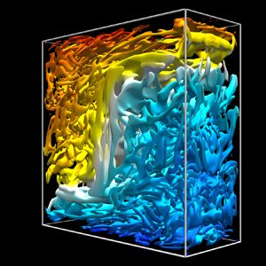The views in figure 7 and supplementary movies 4 and 5 show 3-D perspectives of the isotherms and the $Q_N=0.04$ isosurface (coloured by $T$), whereas figure 8 and supplementary movie 6 are contour plots of $T$ and $Q_N$ in the three midplanes $x=0$, $y=0$ and $z=0$.

Figure 7. Snapshots of isotherms (a) and $Q_N$-criterion at isolevel $Q_N=0.04$ coloured by the temperature (b) at forcing periods $n_\tau =1$, 2, 5 and 10 covering a transient wave-breaking event, with forcing frequency $\omega _f=1.34$ and forcing amplitude $\alpha _f=0.3$. Supplementary movies 4 and 5 animate these over 10 forcing periods.

Figure 8. Snapshots of the isotherms and $Q_N$-criterion along the various vertical and horizontal midplanes at the times indicated during a transient wave-breaking event at $\omega _f=1.34$ and $\alpha _f=0.3$. Each panel consists of the square vertical $y=0$ midplane, with the horizontal $z=0$ midplane above it, and the vertical $x=0$ midplane to its left. Supplementary movie 6 shows an animation over 10 forcing periods.

The snapshots in figures 7 and 8 show a range of small- and large-scale structures in the cavity. These are correlated with hairpin and lambda vortices spawned near the boundary. In the interior, there are also temperature inversions due to the sloshing motion that vary in intensity over the 10 forcing periods and lead to small-scale vortical structures. The localized vortical regions are identified by $Q_N>0$ (shown in red), while localized shear regions are identified by $Q_N<0$ (shown in blue) and are correlated with strong gradients in $T$. At $n_\tau =1$, the flow is spanwise reflection symmetric $\mathcal {K}_{y}$ and invariant to the combined $x$ and $z$ reflection symmetries $\mathcal {K}_{x}\mathcal {K}_{z}$. By $n_\tau \approx 5$, the interior is undergoing wave breaking and all the spatial symmetries have been broken. The broken symmetries are more pronounced in the snapshots at $n_\tau =10$. Symmetry breaking implies the existence of conjugate states, and their presence may lead to heteroclinic dynamics with excursions to and from the various states. This may be at play in the wave-breaking regime. In Yalim et al. (Reference Yalim, Welfert, Lopez and Wu2017), wave breaking was investigated using 2-D simulations over tens of thousands of forcing periods, and intermittent excursions between various states that are typical of heteroclinic dynamics were observed. The time scales involved in heteroclinic dynamics make a detailed investigation in three dimensions prohibitively expensive. Furthermore, wave breaking in three dimensions is qualitatively different from wave breaking in two dimensions; three dimensions involves intense temperature gradients in the spanwise direction, which are absent in the 2-D idealization, and these are necessary for the baroclinic production of the intense tube-like vortex structures that are clearly evident throughout the container in figure 7. In two dimensions, the vorticity only has a single component, resulting in spanwise-invariant vortex sheets.