2.1. Flow configuration

The experimental study from Song & Eaton (Reference Song and Eaton2004) is reproduced numerically for the Reynolds number $Re_{\theta,ref}=13{,}200$. The boundary layer undergoes separation over a rounded step, then reattaches and develops downstream. A representation of the flow configuration is sketched in figure 1. Several works in the literature have simulated this kind of flow but at lower Reynolds numbers. For instance, in the works of Lardeau & Leschziner (Reference Lardeau and Leschziner2011) and Bentaleb et al. (Reference Bentaleb, Lardeau and Leschziner2012), WRLES is performed for a similar geometry (although slightly modified) at almost $Re_\theta =1200$. Radhakrishnan et al. (Reference Radhakrishnan, Piomelli, Keating and Lopes2006) simulated the same flow at higher Reynolds number, $Re_\theta = 13{,}200$, the same as in the present study, but with a much coarser grid than the one considered in ZDES, and employing the standard detached-eddy simulation (DES) as in Nikitin et al. (Reference Nikitin, Nicoud, Wasistho, Squires and Spalart2000) as a WMLES approach. The length of the round step is $L$, the height is $h=0.3L$, and the $^\prime$ symbol is used in length-type variables when normalised by the step length (for instance, $x^\prime = x/L$). The reference station is placed at $x^\prime =-2$, where $Re_{\theta,ref}=13{,}200$ as mentioned earlier. An illustration of the flow configuration is given in figure 4 below, and $x$, $y$ and $z$ are respectively the streamwise, vertical and spanwise directions. It is important to mention that the geometry of the top wall is slightly modified in the present study, as explained in § 2.2.

Figure 1. Schematic representation of the flow configuration.

2.2. Numerical set-up

In the present work, the outer part of the boundary layer is resolved by means of an LES approach using ZDES mode 3 (Deck Reference Deck2012; Renard & Deck Reference Renard and Deck2015a). This method, which is described in Appendix A, employs the Spalart–Allmaras (Spalart & Allmaras Reference Spalart and Allmaras1994) turbulence model as a subgrid-scale (SGS) model, in order to link the SGS stress tensor to the mean field variables. In addition, a thin near-wall RANS layer is acting as a wall model. This method has already been used in other high-fidelity simulation studies, such as in Deck et al. (Reference Deck, Weiss, Pamiès and Garnier2011, Reference Deck, Renard, Laraufie and Sagaut2014a,Reference Deck, Renard, Laraufie and Weissb) and Deck & Laraufie (Reference Deck and Laraufie2013). Figure 2 illustrates the results obtained from a quasi-incompressible ZPG turbulent boundary layer at high Reynolds number employing ZDES mode 3, where very good agreement with experimental data is observed for the mean velocity profile.

Figure 2. Mean velocity profile of a ZPG turbulent boundary at $Re_\theta =15{,}500$ and $Re_\tau = 4900$, from a ZDES mode 3. Experimental results of Vallikivi, Hultmark & Smits (Reference Vallikivi, Hultmark and Smits2015) ($Re_\tau = 4635$) and Österlund (Reference Österlund1999) ($Re_\tau = 4758$) are also included.

This work focuses mainly on the outer layer turbulent structures in out-of-equilibrium conditions. Even though turbulence resolving methods are essential for this type of study, simulations based on the RANS approach have also been carried out in the present work for mean field comparisons. The two eddy-viscosity models considered for the RANS simulations are the Spalart–Allmaras (SA) model (Spalart & Allmaras Reference Spalart and Allmaras1994) and the $k$-$\omega$ shear stress transport (SST) from Menter (Reference Menter1994). Regarding the Reynolds stress model (RSM), the SSG-LRR-$\omega$ (Launder, Reece & Rodi Reference Launder, Reece and Rodi1975; Speziale, Sarkar & Gatski Reference Speziale, Sarkar and Gatski1991; Cécora et al. Reference Cécora, Radespiel, Eisfeld and Probst2015) model is employed in this study. The Reynolds average of a variable $\bullet$ is denoted in this work by $\langle \bullet \rangle$.

The geometry of the computational domain (top wall) has been modified slightly to take into account the side-wall effects present in the wind tunnel, without simulating the side-wall boundary layers. This allows us to reduce the computational effort in ZDES, while keeping the proper pressure coefficient evolution. The method detailed in Vaquero, Renard & Deck (Reference Vaquero, Renard and Deck2019a) has been employed, for which the results are presented in figure 3 for both the Spalart–Allmaras model and ZDES. Also, a comparison is made against a RANS simulation with a flat top and the side-wall boundary layers (SA 3-D), and very accurate results are obtained with ZDES, thus validating the geometry of the top wall for the statistically two-dimensional (2-D) simulations. Moreover, it is interesting to point out the good prediction of the pressure coefficient by ZDES, especially in the separation region.

Figure 3. Pressure coefficient evolution over the bottom wall for different top wall geometries, including a full three-dimensional (3-D) computation with a flat top wall.

Table 1 gathers the grid parameters for ZDES mode 3. Parameters for the other simulations are not included since these are two-dimensional and the grid in the $(x,y)$ plane is identical, i.e. $\Delta x = 0.0108L$ and $\Delta y |_w = 0.000054L$. In the present case, we have taken $L_z = 3.8\delta _{10}$ for the ZDES computation (leading to $N_{xyz} = 290 \times 10^6$, see table 1), which has been verified to be enough to avoid any spanwise correlation. As we remarked in the Introduction, such an investigation at high Reynolds number cannot be tractable with DNS or WRLES, for which it is estimated $N_{xyz}=320\times 10^9$ and $N_{xyz}=16\times 10^9$, respectively. Radhakrishnan et al. (Reference Radhakrishnan, Piomelli, Keating and Lopes2006) also simulated the experiment of Song & Eaton (Reference Song and Eaton2004) using standard DES at the same Reynolds number, but the span was less than half the span in the present work ($L_z = 3 \delta _{ref}$), and the mesh was coarser as well ($N_{xyz}=5.7 \times 10^6$).

Table 1. Grid parameters and numerical domain specifications for ZDES. Here, $\Delta y |_w$ is the spacing in the $y$ direction for the first cell away from the wall. The values given in wall units (superscript $+$) are taken at the most restrictive region of the domain. Quantities $\delta _{in}$, $\delta _{ref}$, $\delta _{0}$ and $\delta _{10}$ correspond to the boundary layer thickness at the inlet, at $x^\prime =-2$ (reference station), at $x^\prime =0$ and at $x^\prime =10$, respectively.

In the ZDES computation, the position of the inlet of the domain is different than in RANS simulations. Instead, the inlet is placed at $x^\prime =-15.7$, whereas in the RANS simulations, the inlet is located further upstream ($x^\prime =-43$). The reason for the inlet being placed further downstream in the ZDES computation is to reduce computational effort since the simulation is three-dimensional. Also, turbulent inflow conditions are used due to the presence of resolved turbulence when using ZDES mode 3. In particular, the synthetic-eddy method (Pamiès et al. Reference Pamiès, Weiss, Garnier, Deck and Sagaut2009; Deck et al. Reference Deck, Weiss, Pamiès and Garnier2011; Laraufie & Deck Reference Laraufie and Deck2013) is employed to generate turbulent structures, and it is coupled with a dynamic forcing method as presented by Laraufie, Deck & Sagaut (Reference Laraufie, Deck and Sagaut2011) that allows accelerating the transition of the injected turbulent structures to become proper turbulent structures of the actual simulation. Regarding the outlet, even though the last station where experimental data of Song & Eaton (Reference Song and Eaton2004) are available is placed at $x^\prime =7$, in all the simulations it is located at $x^\prime =14$, thus allowing for a greater relaxation region.

Two different solvers have been used in the present work. The RANS simulation with the Spalart–Allmaras turbulence model and ZDES mode 3 have been carried out with the solver FLU3M developed at ONERA, which has already been used for high-fidelity simulations (see, for instance, the work of Deck & Laraufie Reference Deck and Laraufie2013; Deck et al. Reference Deck, Renard, Laraufie and Weiss2014b, Reference Deck, Weiss and Renard2018). The simulations with the $k$-$\omega$ SST model and the RSM have been performed utilising the ONERA solver elsA (Cambier, Heib & Plot Reference Cambier, Heib and Plot2013). Even though different solvers are used in this study, the numerics employed in all the simulations are very similar. Moreover, a comparison between FLU3M and elsA simulations using the Spalart–Allmaras model has been made keeping the same numerics, and differences were not noticeable. This allows excluding the use of different solvers as a possible source of error.

The numerics employed in the RANS simulations are the same regardless of both the turbulence model and the solver. The spatial integration is performed through the finite volume method using Roe's scheme and the MUSCL (Monotonic Upstream Scheme for Conservation Laws) approach for flux reconstruction at the cell faces. RANS simulations are steady, and the pseudotemporal integration is computed through an implicit Euler's scheme.

For ZDES, the finite volume method is also used. In the numerical domain, only the lower-wall boundary layer is solved with ZDES mode 3, and the upper-wall boundary layer is treated in RANS (with the Spalart–Allmaras model) thanks to the zonal feature of ZDES. The numerical scheme applied is the AUSM $+$ (P) suggested by Liou (Reference Liou1996) and modified according to Mary & Sagaut (Reference Mary and Sagaut2002). The temporal integration in the ZDES computation is made by means of a Gear's scheme with time step $\Delta t=2.67\times 10^{-7}$ s. In the present simulation, $\Delta t^+ = {\Delta t u_\tau ^2}/{\nu }$ is below 0.2 in the whole domain, which is in accordance with the requirement $\Delta t ^+ < 0.4$ proposed by Choi & Moin (Reference Choi and Moin1994). Also, the inner RANS region is located within $0.1\delta$ from the wall in attached regions, which corresponds to the whole inner layer, as in previous studies (Deck et al. Reference Deck, Renard, Laraufie and Sagaut2014a, Reference Deck, Weiss and Renard2018; Renard & Deck Reference Renard and Deck2015a). Due to the presence of local mean pressure gradients in the flow, the boundary layer thickness is evaluated by employing a method inspired by that used in the work of Spalart & Watmuff (Reference Spalart and Watmuff1993) or Kitsios et al. (Reference Kitsios, Sekimoto, Atkinson, Sillero, Borrell, Gungor, Jiménez and Soria2017). Within the recirculation bubble, the RANS region extends up to a distance from the wall of about $0.1\delta _{x^\prime = 0}$. The mean field comparison to the experimental measurements presented in both § 3.2 and Appendix B confirms the accurate flow prediction obtained using the mentioned definition of the RANS region location.

3.1. Visualisation of the instantaneous flow field

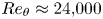
An insight into the flow is presented through the instantaneous field obtained from ZDES. Figure 4 shows the $Q$-criterion (Hunt, Wray & Moin Reference Hunt, Wray and Moin1988) of the flow, and figure 5 presents a numerical schlieren. From the $Q$-criterion, it is observed that turbulence is resolved finely in the outer layer, and the typical hairpin-like structures are recognisable. Also, the boundary layer is thicker than upstream of separation, and turbulent structures are more easily observable in the redevelopment region due to the high increase in Reynolds number ($Re_\theta \approx 13{,}200$ at $x^\prime =-2$, and $Re_\theta \approx 24{,}000$ at $x^\prime =8$). In the numerical schlieren (figure 5), it is possible to identify the typical elongated turbulent structures inclined in the flow direction due to the streamwise velocity shear, which for ZPG turbulent boundary layers are inclined at angle $14^\circ$ according to Marusic & Heuer (Reference Marusic and Heuer2007). Those structures correspond to the large-scale structures of high-Reynolds-number turbulent boundary layers since their sizes are commensurable to the boundary layer thickness. Indeed, as already mentioned, large-scale motions have streamwise lengths $\lambda _x$ of approximately 2–3$~\delta$.

Figure 4. Isosurface of $Q$-criterion for $Q=0.16 ({U_{e}}/{\delta } )_{ref}^2$ coloured by the instantaneous streamwise velocity.

Figure 5. Numerical schlieren $( \sqrt {({\partial \rho }/{\partial x_i})({\partial \rho }/{\partial x_i})} )$ in the $(x^\prime,y^\prime )$ plane, where $\rho$ is the fluid density.

3.2. Comparison to experimental measurements

Integral properties of the mean flow boundary layer as well as mean velocity and Reynolds stress profiles are presented in this section. Comparisons are made not only to the experimental data but also to popular RANS eddy-viscosity models and one RSM (see § 2.2). Regarding the mean quantities displayed in figure 6, ZDES gives excellent agreement with experimental results for the shape factor in the whole domain. Very good agreement is also obtained for the friction coefficient, especially after reattachment, in the redevelopment region, which is the main region of interest in the present study.

Figure 6. Friction coefficient (a) and shape factor (b) evolutions in the streamwise direction.

Concerning the results from the RANS models computations, there are some discrepancies in reproducing the friction coefficient in the redevelopment region. In particular, both the Spalart–Allmaras and $k$-$\omega$ SST models underestimate the friction coefficient and give an increasing trend. This very likely results from the flow being out of equilibrium, whereas these models are calibrated in near-equilibrium conditions. Some differences are also present in the shape factor, where the Spalart–Allmaras model underestimates the shape factor in the recirculation bubble, whereas the other RANS models (and ZDES) are very accurate. This difference for the Spalart-Allmaras model results from a less satisfactory prediction of the displacement and momentum thicknesses (not shown) compared to the other models. Indeed, the friction coefficient is related to the momentum thickness and the shape factor through the Von Kármán equation.

Figures 7–10 present the mean velocity and Reynolds stress profiles for $x^\prime =4$ and $x^\prime =7$, which are located downstream of reattachment, in the relaxation region, which is the main focus of this study. Predictions of mean velocity profile and Reynolds shear stress (figure 7) by ZDES match the experimental measurements very accurately. The boundary layer is not in canonical conditions, as evidenced clearly by the external peak observed in the outer layer for the Reynolds shear stress, which results from the increased turbulent activity in the shear layer after separation. Further downstream, at $x^\prime =7$ (figure 9), ZDES results are again in strong agreement with experimental measurements. The boundary layer is recovering from non-equilibrium induced by excess turbulent activity resulting from the shear layer in the separated region, although canonical conditions have not been reached yet. This is observable in the profile of Reynolds shear stress, where the outer peak is still present (both in the experiment and in the ZDES computation), although it has decreased significantly compared to station $x^\prime =4$. Also, in the mean velocity profile at $x^\prime =7$, the log region is more clearly identifiable, and extends in a vast extension of the mean velocity profile due to the high Reynolds number at this station, which is about $Re_\theta = 23{,}400$.

Figure 7. Mean velocity (a) and Reynolds shear stress (b) profiles at $x^\prime =4$. The dashed vertical line indicates the position of the RANS/LES interface. For ZDES, the Reynolds shear stress profile is split into modelled (dotted) and resolved (dashed) contributions.

Figure 8. Streamwise (a) and wall-normal (b) velocity fluctuations profiles at $x^\prime =4$. The inner RANS region for ZDES is shaded in grey.

Figure 9. Mean velocity (a) and Reynolds shear stress (b) profiles at $x^\prime =7$. The dashed vertical line indicates the position of the RANS/LES interface. For ZDES, the Reynolds shear stress profile is split into modelled (dotted) and resolved (dashed) contributions.

Figure 10. Streamwise (a) and wall-normal (b) velocity fluctuations profiles at $x^\prime =7$. The inner RANS region for ZDES is shaded in grey.

RANS results in the reattachment region are less accurate. The mean velocity profile at $x^\prime =4$ presents a small underestimation in the inner layer for both eddy-viscosity models, and is better reproduced by the RSM. Regarding the Reynolds shear stress at this same station, all the models give an outer peak, but its level is clearly underestimated by the Spalart–Allmaras model. The peak from the $k$-$\omega$ SST model is closer to the experiment, but still underestimated, whereas the RSM predicts a slightly overestimated Reynolds shear stress for the peak. An important discrepancy between RANS computations and ZDES is observed regarding the position of the mentioned outer peak. In fact, ZDES adequately predicts the peak to be around $y\approx 0.32\delta$, which is very similar to the experiment, but RANS computations provide a lower location of the peak, being at about $y\approx 0.24\delta$ for the three RANS models considered. This misprediction of the peak location is very likely responsible for the departure from experimental data in the RSM mean velocity profile, with an underestimation around $y\approx 0.1\delta$ followed by a minor overestimation around $y\approx 0.5\delta$.

At $x^\prime =7$, predictions from RANS models are closer to the experiment because the boundary layer is relaxing from non-equilibrium conditions. However, the same discrepancy as the one just described for $x^\prime =4$ is still observed for RANS computations compared with ZDES and the experiment, although to a lesser extent. Predictions of Reynolds shear stress levels from RANS models are in better agreement at this station, but the position of the peak remains moderately shifted closer to the wall. Concerning the mean velocity profile, a better agreement is also observed at this station from RANS simulations, and discrepancies are limited to a small underestimation of the mean velocity in the log region by the $k$-$\omega$ SST model, and a slight overestimation in the wake region by the Spalart–Allmaras model.

The profiles of $u_{rms}$ and $v_{rms}$ at $x^\prime =4$ and $x^\prime =7$ are displayed in figures 8 and 10, respectively. The wall-normal velocity fluctuations at $x^\prime =4$ are reproduced accurately by ZDES, and fluctuations in the streamwise direction are slightly underestimated below $y\approx 0.5\delta$. Further downstream, at $x^\prime =7$, the velocity fluctuations in both the streamwise and wall-normal directions are fairly well reproduced, although there is a moderate underestimation compared to the experimental results. The RSM, conversely, does not properly predict velocity fluctuations at these stations, regarding both the levels and the trend. At both stations, $u_{rms}$ and $v_{rms}$ are below the experimental values in the whole profile, and a faster decay away from the wall is predicted by this model.

Profiles of mean velocity and Reynolds shear stress at two stations upstream of separation and at the recirculation region are discussed further in Appendix B, for the sake of conciseness. Results from the ZDES computation are again in fairly good agreement with the experimental measurements, and some non-canonical features of the flow are well reproduced in this simulation, which is not the case for all the RANS simulations considered. Also, in the recirculation bubble, the inflexion point is well reproduced by ZDES in terms of both velocity magnitude and position from the wall, whereas less accurate results are provided by the RANS computations. Another interesting aspect to point out is the prediction of negative Reynolds shear stress ($-\langle u^{\prime } v^{\prime } \rangle < 0$) very near the wall, which is observed in neither the ZDES profile nor the experiment (see figure 23).

3.3. Spectral analysis of streamwise velocity fluctuations

The spectral content of velocity fluctuations in the streamwise direction is studied in this subsection at different domain stations. In the study of turbulent boundary layers, it is common to focus on the spatial length scales of coherent structures. However, the evolution of the boundary layer in the streamwise direction makes this a non-homogeneous direction, therefore the analysis of streamwise coherent structures is performed by utilising time signals of the streamwise velocity at a given spatial position and a link between frequency and streamwise wavenumber, which is given assuming Taylor's hypothesis; see, for instance, the work of Renard & Deck (Reference Renard and Deck2015b).

The one-sided power spectral density (PSD) for $\langle u^{\prime 2} \rangle = (u_{rms})^2$ is given by $G_{uu;f}(f)$, expressed such that

(3.1)\begin{equation} \langle u^{\prime 2} \rangle = \int_{0}^{+\infty} G_{uu;f}(f) \,\mathrm{d} f. \end{equation}

It is very common to present the PSD in logarithmic scale for the frequency. It is then usually chosen to plot the pre-multiplied PSD, $f\,G_{uu;f}(f)$, because the area under the curve of $f\, G_{uu;f}(f)$ in a semi-logarithmic scale at a given position $d_w/\delta$ is proportional to the contribution to $\langle u^{\prime 2} \rangle$ at the considered $d_w/\delta$.

In the present study, the signal of streamwise velocity has been collected from ZDES for a total time $T\approx 430 ( \delta / U_e )_{ref}$. That recording time is long enough to capture the low-frequency dynamics of the flow since it corresponds to around 30 periods of time for the flapping mode. Figures 12 and 13 display the distribution of the pre-multiplied PSD, estimated using Welch's method (Welch Reference Welch1967), at positions $P_1$, $P_3$ and $P_6$, located at $x^\prime = 0$, $x^\prime = 1$ and $x^\prime = 7$ (and following the mesh lines, see figure 11). The boundary layer quantities $\delta$, $U_e$ and $\nu /u_\tau$ employed for normalisation at station $P_3$ (figure 13) are taken from station $P_1$ since station $P_3$ is located within the recirculation bubble. In fact, in the recirculation bubble, the boundary layer is completely separated, and $\delta$ and $\nu /u_\tau$, though calculable, do not play the same role in the normalisation from a physical point of view. Hence in order to make proper comparisons, the values at $P_1$ have been employed at $P_3$, but $P_6$ is located downstream of reattachment, therefore at $P_6$, values of $\delta$, $U_e$ and $\nu /u_\tau$ are computed locally.

Figure 11. Positions of data extraction for spectral analysis.

Figure 12. Pre-multiplied spectrum of streamwise velocity fluctuations at $P_1$ (see figure 11). The shaded area indicates the RANS region.

Figure 13. Pre-multiplied spectrum of streamwise velocity fluctuations at $P_3$ (a) and $P_6$ (b) (see figure 11). The shaded area indicates the RANS region. The values of $\delta$, $U_e$ and $\nu /u_\tau$ at $P_3$ are taken as those from $P_1$ since the $P_3$ station is located within the recirculation bubble.

The convection velocity could be evaluated by using the local mean velocity, or even more sophisticated convection velocities such as the one proposed by Deck et al. (Reference Deck, Renard, Laraufie and Sagaut2014a) based on the two-point two-time correlation coefficient, or the one suggested by Renard & Deck (Reference Renard and Deck2015b), which is dependent on turbulent structures length scale. Even though we have mentioned the use of Taylor's hypothesis for linking frequency content and spatial length scales, such a hypothesis cannot be applied in the backward flow region since turbulent velocity fluctuations and the mean back-flow velocity are of the same order of magnitude (Simpson Reference Simpson1989). For this reason, plots in figures 12 and 13 are given in frequency content (even for $P_1$ and $P_6$), with $f^+=f \nu / u_\tau ^2$. However, since $\lambda _x / \delta = U_c /(f\delta )$, it has been chosen to plot the PSD as a function of the inverse of the frequency because $U_e/(f\delta )$ is representative of $\lambda _x/\delta$ when Taylor's hypothesis may be applied (as with $P_1$ and $P_6$). Even though it is not strictly the same because using $U_c(d_w/\delta )=U_e$ as the convection velocity would not be very suited, $U_c$ remains a fraction of $U_e$ even in the near-wall region (Deck et al. Reference Deck, Renard, Laraufie and Sagaut2014a; Renard & Deck Reference Renard and Deck2015b).

At stations $P_1$ and $P_6$, analysis of the pre-multiplied PSD as a function of the wavenumber ($k_x\,G_{uu;k_x}(k_x)$) has been performed using the two-point two-time correlation coefficient for the convection velocity as described by Deck et al. (Reference Deck, Renard, Laraufie and Sagaut2014a). However, it is not shown since changes to the figures presented are limited to a slight shift of the energy content to lower wavelengths. Nevertheless, values of $\lambda _x/\delta$ from the plot of $k_x\,G_{uu;k_x}(k_x)$ will be indicated in the discussion.

The turbulent content before separation, presented in figure 12, shows a quite homogeneous distribution in a wide range of scales at $d_w \approx 0.2\delta$, with length scales from $\lambda _x = 0.4\delta$ to $\lambda _x = 40\delta$. It is interesting to notice that turbulent fluctuations at large scales are still present within the RANS region, but small structures present in the LES region are dissipated in the RANS region. This is not surprising because, as recalled by Renard & Deck (Reference Renard and Deck2015c), the fraction of resolved Reynolds shear stress decreases gradually within the RANS region. As already mentioned, $U_e \geq U_c$ across the boundary layer profile, so $U_e/(f\delta ) \geq \lambda _x / \delta$, which causes the PSD in figure 12 to be shifted slightly towards greater values in the vertical axis, when plotted against $U_e/(f\delta )$ instead of $\lambda _x/\delta$. For instance, the length scale associated with $U_e/(f\delta ) \approx 10$ is $\lambda _x/\delta \approx 8\unicode{x2013}9$ instead. It is also important to notice that values of $\lambda _x/\delta$ with important energy content are significantly higher than those for very large-scale motions (VLSM) in ZPG turbulent boundary layers (for which $\lambda _x$ is 5–6 $\delta$).

The spectral content is very different within the recirculation bubble, as illustrated in figure 13. Again, energy is distributed in a broad range of scales. It is important to mention that for this station, $U_e/(f\delta )$ may not be as accurate as at $P_1$ for estimating $\lambda _x/\delta$ because the values of $\delta$, $U_e$ and $\nu /u_\tau$ used are those from $P_1$. It is recalled that this choice is made for the sake of comparison because the boundary-layer-like thickness and the friction velocity at $P_3$ do not represent an adequate scaling within the recirculation bubble. Energy levels at $P_3$ are much more important than at $P_1$ (the range of values in the colourbar is not the same), and we can observe three localised energy sites for $U_e/(f\delta )=10$ and above that likely correspond to the shear layer mode and the shedding mode, as will be described later, in § 4.2. Regarding the flapping mode, the present flow configuration does not discern clearly this mode from the others. Indeed, the flapping mode is characterised by $St=fL_R/U_{\infty } = 0.12\unicode{x2013}0.18$, and the shear layer mode by $St_\theta = f\theta _{sep}/U_{\infty } =0.012$. In the flow field studied, $U_\infty = U_{ref}$ and $\theta _{sep}/L_R \sim 0.1$, hence although the shear layer mode and the flapping mode have certainly distinct Strouhal numbers, in the present case, their absolute characteristic frequencies are very close to each other.

In the relaxation region (figure 13), the PSD changes significantly with respect to the separated region, and some similarities to the $P_1$ station are recovered. In particular, energy in the RANS region is observable again, and energy levels are lowered with respect to those in the separated region, and they are closer to, yet greater than, those upstream of separation. In the outer layer, energy is more concentrated for structures whose length scales range from $\lambda _x = 1.5\delta$ to $\lambda _x = 9\delta$. However, the peak location related to VLSM falls within the RANS region and is not observed, evidently, as was the case at $P_1$. The energy in the outer layer at $P_6$ is significantly greater and more broadly distributed across the boundary layer. There is still some important turbulent activity even at $d_w = 0.5\delta$. This is probably the result of the high Reynolds number at this station, which is $Re_\theta =23{,}400$ and $Re_\tau = 6285$, but some trace of the high outer layer activity from the shear layer at separation probably influences the turbulent content at this station. Indeed, the mean velocity profile is close to canonical ZPG conditions, but the Reynolds shear stress profile still shows an external peak as a consequence of the excess of turbulence created by boundary layer separation (see figure 9).

4.1. Spatial evolution of turbulence production

The shear layer in the separated region creates an excess of turbulence that is convected in the outer part of the boundary layer once reattachment takes place. In order to analyse better the extent of the shear layer trace, the mean field of the whole TKE production term as in equation (4.1) is here presented. The production term for the turbulent kinetic energy $k$ in a statistically two-dimensional flow is given by

(4.1)\begin{equation} \mathcal{P}_k ={-}\langle u^{\prime} v^{\prime} \rangle \left( \frac{\partial \langle u \rangle}{\partial y} + \frac{\partial \langle v \rangle }{\partial x}\right) + (\langle v^{\prime 2} \rangle - \langle u^{\prime 2} \rangle) \frac{\partial \langle u \rangle}{\partial x}. \end{equation}

Results from RANS simulations are included as well, for comparison purposes. In the case of the two eddy-viscosity models (Spalart–Allmaras and $k$-$\omega$ SST), for which Boussinesq's hypothesis (A1) is considered, the TKE production may be written as

(4.2)\begin{equation} \mathcal{P}_k=\nu_t \left( \frac{\partial \langle u \rangle}{\partial y} + \frac{\partial \langle v \rangle}{\partial x} \right)^2 + 2 \nu_t \left( \frac{\partial \langle u \rangle}{\partial x} - \frac{\partial \langle v \rangle}{\partial y} \right) \frac{\partial \langle u \rangle}{\partial x}, \end{equation}

where $\nu _t = \mu _t /\rho$, with $\mu _t$ the eddy viscosity and $\rho$ the fluid density. It is important to mention that the production of TKE considered in (4.1) corresponds to the true production, and in (4.2) to its evaluation with Boussinesq's hypothesis, which may differ from the production term considered for the transport equation of TKE, $k$, in the $k$-$\omega$ SST model.

The field of $\mathcal {P}_k$, as in (4.1) and (4.2), is displayed in figure 14 for all the RANS simulations and ZDES. For the latter, the total production is considered, i.e. the sum of the resolved production, as in (4.1), and the modelled one, as in (4.2). The results obtained are significantly different depending on the RANS model considered. In all cases, there is a clear excess of $\mathcal {P}_k$ away from the wall resulting from the turbulence enhancement happening in the shear layer. Such an excess results in a second peak in the outer part of wall-normal profiles of TKE production. However, this excess of $\mathcal {P}_k$ disappears in shorter distances for the two eddy-viscosity models, which seem to be too diffusive, especially in the Spalart–Allmaras computation. Indeed, the last position of the outer peak of $\mathcal {P}_k$ detected for ZDES is located at $x^\prime \approx 11$, whereas for the $k$-$\omega$ SST and Spalart–Allmaras models, the secondary peak disappears beyond $x^\prime \approx 6$ and $x^\prime \approx 3.5$, respectively, and for the RSM the outer peak is still present at the end of the computational domain. The discrepancies observed in the friction coefficient after reattachment, where RSM and ZDES are significantly more accurate than the two eddy-viscosity models (see figure 6), are very likely related to the higher dissipation of $\mathcal {P}_k$ for the eddy-viscosity models. In fact, TKE production plays a key role in the friction coefficient, which has been evidenced explicitly, for instance, in the mean skin friction decomposition suggested by Renard & Deck (Reference Renard and Deck2016).

Figure 14. Mean field of TKE production $\mathcal {P}_k$ with all terms considered as in (4.1). From (a)–(d): Spalart–Allmaras model, $k$-$\omega$ SST model, RSM and ZDES. Pink dots indicate the position of the outer peak. Yellow-filled dots indicate the position of the furthest-downstream outer peak. The white line corresponds to the boundary layer thickness ($y^\prime = \delta ^\prime$, with $\delta ^\prime = \delta /L$ the normalised local boundary layer thickness). The vertical axis is magnified for visualisation purposes.

Quite similar results are obtained between the RSM computation and ZDES, despite some discrepancies being present. Even though for both simulations the excess of $\mathcal {P}_k$ disappears very far downstream, the RSM appears to be not diffusive enough since the field is narrower around the secondary peak. This is consistent with the profiles of normal Reynolds stresses in the redevelopment region (figures 8 and 10), which are also narrower for RSM than for ZDES and the experiment. Also, the furthest position for the outer peak detected in ZDES is at $x^\prime \approx 11$, whereas the outer peak seems to be still present at the end of the computational domain for the RSM simulation. Moreover, in the RSM computation, the outer peak is positioned further away from the wall (in outer scale) in the boundary layer until $x^\prime \approx 7$, and then it seems to be placed at $y/\delta \approx 0.5$. Thus the distance between the wall and the outer peak is monotonically increasing with $x^\prime$, whereas in ZDES, the wall-normal distance of the peak does not change significantly beyond $x^\prime =6$. This means that the further downstream of $x^\prime = 6$, the lower the outer peak is located within the boundary layer in outer scale since the boundary layer thickness keeps increasing.

The production term of turbulent kinetic energy presented in figure 14 has been integrated in the $y$ direction in order to analyse the streamwise evolution of the bulk production of TKE, $\mathbb {P}_{k}$. As illustrated in figure 15, different evolutions of the bulk TKE production are provided by the different models. More precisely, it is interesting to notice the underestimation obtained from the Spalart–Allmaras model, which could have been inferred from the previous analysis of figure 14. On the contrary, a more surprising result is obtained from the $k$-$\omega$ SST model. This model predicts an evolution of the bulk TKE production that is not only in better agreement with ZDES, but also very close to the evolution obtained from the RSM model, despite the important differences between the two models regarding the spatial distribution of the TKE production (figure 14), mainly concerning the outer peak. One may suppose that the fact of having the same transport equation for the specific TKE dissipation rate in both models is partly responsible for the close behaviour between them. It is also observed that even though both models provide an accurate prediction of the bulk TKE production levels with respect to ZDES, there is a slight discrepancy in the trend, which results in minor underestimation and overestimation at the beginning and the end of the redevelopment region, respectively.

Figure 15. Streamwise evolution of the bulk production of TKE, $({\mathbb {P}_{k}}/{U_{ref}^3})\times 10^3$, where $\mathbb {P}_{k} (x^\prime ) = \int _0 ^{+\infty } \mathcal {P}_k (x^\prime,y) \,\mathrm {d} y$.

4.2. Spectral analysis of turbulence production

In the previous subsection, it was observed that there is a trace in production of turbulent kinetic energy from the shear layer in the separated region that is still visible far downstream, until $x^\prime \approx 11$. In this subsection, the production term of TKE is studied by means of a spectral analysis of turbulence at some stations in the flow. For ZPG turbulent boundary layers, some of the terms may be neglected in (4.1), and the production can be expressed as (considering $y$ the wall-normal direction)

(4.3)\begin{equation} \mathcal{P}_k ={-}\langle u^{\prime} v^{\prime} \rangle\,\frac{\partial \langle u \rangle}{\partial y}, \end{equation}

which is the expression that will be employed in the spectral analysis presented here. Indeed, for the flow studied in this work, the term considered in (4.3) remains the most dominant term in the whole domain.

The spectral analysis of $\mathcal {P}_k$ is performed through the Reynolds shear stress according to (4.3). Signals of $u(t)$ and $v(t)$ are recorded for the same duration $T \approx 430 ( \delta /U_e )_{ref}$ as in subsection 3.3. According to Deck et al. (Reference Deck, Renard, Laraufie and Weiss2014b), one can write

(4.4)\begin{equation} \langle u^\prime v^\prime \rangle = \int_{0}^{+\infty} 2\,\mathrm{Re} (S_{uv;f}(f))\, \mathrm{d} f = \int_{0}^{+\infty} G_{uv;f}(f) \,\mathrm{d} f , \end{equation}

where $\mathrm {Re}(\bullet )$ denotes the real part, and $G_{uv;f} = 2\,\mathrm {Re} ( S_{uv;f} )$ is the real part of the cross-PSD. Finally, according to (4.3) and (4.4), the production may be expressed as

(4.5)\begin{equation} \mathcal{P}_k ={-}\int_{0}^{+\infty} \frac{\partial \langle u \rangle}{\partial y}\,G_{uv;f}(f)\, \mathrm{d} f. \end{equation}

The co-spectrum of $\mathcal {P}_k$ is presented at stations $P_1$, $P_3$ and $P_6$ in figures 16, 17(a) and 17(b), respectively. In these figures, the cross-PSD is pre-multiplied by the frequency as explained previously in § 3.3 for $G_{uu;k_x}$, and by the wall distance as well. Indeed, the total production of TKE across the whole boundary layer profile (per boundary layer thickness) is

(4.6) \begin{equation} \mathcal{P}_{tot} = \int_0 ^{+\infty} \mathcal{P}_k \,\mathrm{d}\!\left( \frac{d_w}{\delta} \right) = \int_{-\infty} ^{+\infty} \frac{d_w}{\delta}\,\mathcal{P}_k \,\mathrm{d}\!\left( \ln \left( \frac{d_w}{\delta} \right) \right),\end{equation}

thus the area under the curve of $({d_w}/{\delta })\,\mathcal {P}_k( d_w /\delta )$ in logarithmic scale is directly proportional to the contribution to the whole TKE production across the boundary layer profile.

Figure 16. Pre-multiplied co-spectrum of $\mathcal {P}_k$ at $P_1$ (see figure 11). The shaded area indicates the RANS region. The solid lines show the pre-multiplied PSD of $\langle u^{\prime 2} \rangle$ as in figure 12.

Figure 17. Pre-multiplied co-spectrum of $\mathcal {P}_k$ at $P_3$ (a) and $P_6$ (b) (see figure 11). The shaded area indicates the RANS region. The solid lines show the pre-multiplied PSD of $\langle u^{\prime 2} \rangle$ as in figures 13(a) and 13(b). The white dashed lines indicate $U_e/(f\delta )=8.5$, 17 and 34. The values of $\delta$, $U_e$ and $\nu /u_\tau$ at $P_3$ are taken as those from $P_1$ since the $P_3$ station is located within the recirculation bubble.

As in the case of the spectral analysis of streamwise velocity fluctuations (§ 3.3), analysis of the cross-PSD as a function of the wavelength has also been performed at stations $P_1$ and $P_6$, and the relevant results are recalled in the present discussions even if figures are not shown. In particular, even though the order of magnitude of $U_e /(f \delta )$ is representative of $\lambda _x/\delta$ at stations $P_1$ and $P_6$, true values of the wavelength will be given. At $P_3$, the values of $U_e$, $\delta$ and $\nu /u_\tau$ employed are those of station $P_1$ for the same reasons exposed in § 3.3.

The spectral content of $\mathcal {P}_k$ upstream of separation, displayed in figure 16, evidences an important activity of turbulent structures of sizes ranging from $\lambda _x \approx 0.7\delta$ to $\lambda _x \approx 5\delta$ located around $d_w = 0.13\delta$. The contributions of VLSM, which were identified clearly in the PSD of $\langle u^{\prime 2} \rangle$, are also observed, with wavelengths reaching $\lambda _x = 20 \delta$, although levels are slightly lower. There is also some weak activity in $\mathcal {P}_k$ at higher locations in the boundary layer, mainly between $d_w=0.3\delta$ and $d_w=0.8\delta$.

When looking at the spectral content of $\mathcal {P}_k$ within the recirculation bubble, the distribution changes completely. Figure 17(a) displays the cross-PSD of $\mathcal {P}_k$ at station $P_3$. Similarly to the case of $G_{uu;f}$ discussed in § 3.3, turbulent activity is concentrated in the outer part, where the shear layer resulting from separation is located. It is important to point out that levels in the legend are much greater than in figures 16 and 17(b). A broad range of frequencies (scales) participates in the production of TKE. As observed, frequencies from $U_e/(f\delta )=1$ to $U_e/(f\delta )=7$ contribute the most in terms of cross-PSD levels, but important values are observed even beyond $U_e/(f\delta )=100$. According to the frequency of the shear layer, three peaks on the cross-PSD are highlighted. Based on the Strouhal number $St_\omega =f\delta _\omega / \bar {U}$ (where $\bar {U}=0.5( \langle u \rangle _{min} + \langle u \rangle _{max} )$ denotes the shear velocity), the corresponding frequency is represented in figure 17(a), for which $U_e/(f\delta )= 8.5$, and also $U_e/(f\delta )= 17$ and $U_e/(f\delta )= 34$ are indicated. Thus the two lower-frequency peaks (higher values of $U_e/(f\delta )$) likely correspond to the subharmonics due to vortex pairing since the frequency is respectively twice and four times that of the shear layer mode ($St_\omega = 0.135$).

Downstream of reattachment (figure 17b), the cross-PSD of $\mathcal {P}_k$ recovers some of the mentioned features for the station $P_1$. A contribution to production around $d_w=0.13\delta$, which is negligible in figure 17(a), is again present, for which large structures are responsible; structures in this region have sizes from $\lambda _x \approx \delta$ up to $\lambda _x \approx 10 \delta$. The largest structures correspond to VLSM, already identified in § 3.3, and a small peak appears for slightly smaller structures, for which $\lambda _x = 3\delta$. Even if the present station is located far enough away to recover the mentioned features, the main contribution to $\mathcal {P}_k$ remains the high turbulent activity in the outer part, which is the trace of the shear layer at separation. The levels of the cross-PSD are much higher than at $d_w=0.13\delta$, and the contribution is quite broadly distributed in a wide range of wavelengths. The longest structures have $\lambda _x /\delta >10$, and smaller structures, of $\lambda _x /\delta$ down to $0.2$, are observable. Small structures of $\lambda _x = 0.4 \delta$ are also observed upstream of separation (figure 16), but in the recovery region, they are located further away from the wall.

4.3. Friction coefficient

Even though the friction coefficient is a wall quantity, several studies have focused on the interaction between the outer layer and the inner layer, as well as on the contribution to the friction coefficient of large turbulent motions located in the outer layer. According to Balakumar & Adrian (Reference Balakumar and Adrian2007), at high Reynolds numbers, about 40–50 % of the contribution to the Reynolds shear stress at $y>0.1\delta$ comes from turbulent structures with wavelength $\lambda _x > 3\delta$, and in the present study, the LES region corresponds approximatively to $y>0.1\delta$. Also, studies on the friction coefficient decomposition (see, for instance, Fukagata, Iwamoto & Kasagi Reference Fukagata, Iwamoto and Kasagi2002; Renard & Deck Reference Renard and Deck2016) have highlighted the relevance of the Reynolds shear stress contribution. As an example, Deck et al. (Reference Deck, Renard, Laraufie and Weiss2014b) employed the decomposition from Fukagata et al. (Reference Fukagata, Iwamoto and Kasagi2002) to identify that turbulent structures for which $\lambda _x > \delta$ contribute to more than $60\,\%$ of the second term of the friction coefficient decomposition from Fukagata et al. (Reference Fukagata, Iwamoto and Kasagi2002), which is the most relevant term in the friction coefficient, since it represents more than $80\,\%$ of the total friction coefficient.

Before studying the friction coefficient, the reverse flow is analysed by the fraction of time for which the flow moves downstream, $\gamma _u = t( u > 0 ) / T$, and it is displayed in figure 18, for the first cell away from the wall, because of the no-slip condition at the wall. According to Simpson (Reference Simpson1981), there are several states of boundary layer separation that may be identified: incipient detachment (ID) for $\gamma _u = 0.99$, intermittent transitory detachment (ITD) for $\gamma _u = 0.80$, and transitory detachment (TD) for $\gamma _u = 0.50$. Simpson (Reference Simpson1981) defined another state as detachment (D), based on the mean wall shear stress $\langle \tau _w \rangle$, instead of the fraction of time for which the flow moves downstream. Thus detachment appears when $\langle \tau _w \rangle = 0$, and several studies have shown that TD and D take place at the same location (see, for instance, the work of Simpson Reference Simpson1989; Na & Moin Reference Na and Moin1998). The parameter $\gamma _u$ is a classical quantity very often analysed in turbulent boundary layer separation studies (Simpson Reference Simpson1989; Na & Moin Reference Na and Moin1998; Driver, Seegmiller & Marvin Reference Driver, Seegmiller and Marvin1987; Mohammed-Taifour & Weiss Reference Mohammed-Taifour and Weiss2016, Reference Mohammed-Taifour and Weiss2021; Elyasi & Ghaemi Reference Elyasi and Ghaemi2019), and according to Simpson (Reference Simpson1989), it is a feature that should be documented in this kind of work. It may also be a quantity of practical interest for the experimental detection of separation onset and reattachment (see, for instance, Mohammed-Taifour et al. Reference Mohammed-Taifour, Schwaab, Pioton and Weiss2015; Weiss, Mohammed-Taifour & Schwaab Reference Weiss, Mohammed-Taifour and Schwaab2015).

Figure 18. Evolution of the fraction of time for which the flow moves downstream ($\gamma _u$) at the first cell away from the wall, and friction coefficient skewness near the reattachment region and further downstream. Here, $S_{{C_f}^\prime, ZPG}$ is taken from a ZPG turbulent boundary layer at $Re_\theta = 13{,}000$.

The skewness of the friction coefficient is also presented in figure 18, normalised by the value obtained for a ZPG turbulent boundary layer at $Re_\theta =13{,}000$ also using ZDES mode 3. Since the focus is set on the redevelopment and relaxation of the boundary layer towards ZPG canonical flow, the authors have chosen to use the mentioned normalisation. The analysis of this quantity gives relevant information about the near-wall fluctuations, and it is an essential quantity to study the influence of outer layer large scales on inner layer small scales in high-Reynolds-number wall-bounded turbulent flows (Mathis et al. Reference Mathis, Marusic, Hutchins and Sreenivasan2011).

As observed in figure 18, $\gamma _u$ is significantly low within the recirculation bubble, reaching values of about 0.17 for the small plateau at $1.1< x^\prime < 1.3$. Downstream, $\gamma _u$ increases monotonically, even after reattachment (where $\gamma _u=0.5$), and reaches $\gamma _u=1$ at some point between $x^\prime =1.7$ and $x^\prime =2.5$, downstream of which almost no reverse flow is observed. It is interesting to notice that in the recirculation bubble, there is still some downstream flow ($\gamma _u >0$), something that is also observed, for instance, in the DNS of Na & Moin (Reference Na and Moin1998), because the velocity fluctuations and the mean velocity are of the same order of magnitude in the recirculation bubble (Simpson Reference Simpson1989). Another aspect worth mentioning is the high values of $\gamma _u$ upstream of $x^\prime =1.1$, that reach $\gamma _u > 0.5$. It is the consequence of a very tiny recirculation bubble located in the corner of the rounded step resulting from this sharp geometry change, and it is similar to the secondary recirculation identified in backward-facing step studies (such as in Le, Moin & Kim Reference Le, Moin and Kim1997).

An increase of the skewness of the friction coefficient ($S_{{C_f}^\prime }$) within the recirculation bubble in the streamwise direction is observable as well. As already specified, the skewness is normalised by the value in a ZPG turbulent boundary layer flow, simulated with the same approach. In figure 18, the skewness varies significantly: within the recirculation bubble, it takes mainly negative values and increases from $S_{{C_f}^\prime } \approx -3S_{{C_f}^\prime,ZPG}$ until reaching $S_{{C_f}^\prime } \approx S_{{C_f}^\prime,ZPG}$ at the reattachment point. Contrary to $\gamma _u$, downstream of $x^\prime =1.05$, the skewness seems to increase monotonically inside the recirculation bubble, even surpassing the ZPG value downstream of reattachment, up to a maximum of about $3S_{{C_f}^\prime,ZPG}$, and then it decreases, almost reaching the ZPG level, although it is not yet attained at $x^\prime =7$. It is interesting to notice that it is around $x^\prime =7$ where the outer peak in $\mathcal {P}_k$ changes its trend in the way described in § 4.1. This shows that non-equilibrium conditions are significant upstream of $x^\prime \approx 7$, and downstream the boundary layer is close to near-equilibrium. Such a result is evidenced in the evolution of both the outer peak of $\mathcal {P}_k$ and $S_{{C_f}^\prime }$, contrary to that of $\gamma _u$. Near $x^\prime =1$, the skewness is significantly greater than it is around $x^\prime =1.1$, and it decreases right downstream, which is in contrast with the behaviour described earlier, but this is likely due to the presence of the small secondary recirculation bubble mentioned before.

The probability density function (PDF) of the friction coefficient is presented in figure 19 around the reattachment region and at three different locations downstream (stations $P_4$, $P_5$ and $P_6$), and in figure 20 as normalised profiles at different streamwise positions. The PDF is very narrow near $x^\prime =1$ and then broadens ($C_{f,rms}$ increases) in the recirculation bubble until $x^\prime =1.3$, downstream of which it seems to maintain a similar width that changes very slowly. Very far downstream, at $x^\prime =7$, the PDF has clearly narrowed ($C_{f,rms}$ has decreased) and resembles the most what is observed in a ZPG turbulent boundary layer from ZDES. For $1.1 < x^\prime < 1.3$, the flow is reversed and the friction coefficient increases in magnitude (it decreases in figure 19), which suggests that a stronger reversed flow develops. However, the PDF is broader and $C_{f,rms}$ increases as well in this region, which indicates that some downstream flow is still present, as already mentioned. The increase in $C_{f,rms}$ is enough to compensate the stronger reversed flow such that a plateau is observed for $\gamma _u$.

Figure 19. Probability density function of the mean friction coefficient near the reattachment region and further downstream. The continuous line indicates streamwise evolution of the mean friction coefficient. The dashed lines indicate streamwise evolution of the friction coefficient root-mean-square. Stations $P_4$, $P_5$ and $P_6$ are located respectively at $x^\prime = 2.5$, $x^\prime = 4$ and $x^\prime =7$.

Figure 20. Probability density function of the friction coefficient at different streamwise positions. The black dashed line corresponds to a ZPG turbulent boundary layer at $Re_\theta = 13{,}000$.

From figure 20, it is possible to observe the change in the position of the peak of the PDF. At $x^\prime =1.2$, the peak is located the most to positive values of $\tau _w^\prime = \tau _w - \langle \tau _w \rangle$ when normalised with $\tau _{w,rms}$, and it shifts to negative values upstream of $x^\prime =1.63$. Then from $x^\prime =2.5$ to $x^\prime =7$, the peak is shifted again back to higher values of $\tau _w^\prime /\tau _{w,rms}$, although it remains at negative levels of $\tau _w^\prime /\tau _{w,rms}$. This behaviour corresponds to what has already been described for the skewness in figure 18. Indeed, for this kind of PDF distribution, a negative skewness will result in a shift of the peak position to positive values of $\tau _w^\prime /\tau _{w,rms}$, and vice versa. At the furthest position presented, the PDF resembles very accurately that of the ZPG boundary layer. Moreover, the high values of skewness identified in figure 18, which overcome by far the ZPG value, are also evidenced clearly in the shape of the PDF at $P_4$ in figures 19 and 20. In particular, in figure 20, the relaxation towards near-equilibrium conditions is clearly evidenced. It is also interesting to notice that at the position of minimum friction coefficient, which is $x^\prime =1.3$, the skewness is $S_{{C_f}^\prime }\approx -S_{{C_f}^\prime,ZPG}$, which means that the skewness is the same as in ZPG conditions, but with the opposite sign due to the contrary flow direction.