


1. Introduction
Oscillatory flows are one of the fundamental problems in classical fluid dynamics due not only to their underlying basic physics, but also to their applications. These types of flows can be induced by different means, with those induced by the motion of boundaries being the most widely studied. The simplest case corresponds to a pure hydrodynamic flow induced by an oscillating rigid plate in a semi-infinite Newtonian fluid. This problem is referred to as the Stokes problem, named after G. Stokes, who first studied it in 1851 (Stokes Reference Stokes1851). Analogously, oscillatory flows in cylindrical configurations can be induced by torsional (Rivero et al. Reference Rivero, Garzón, Núñez and Figueroa2019) or axial movements (Drazin & Riley Reference Drazin and Riley2006). In contrast, oscillatory flows in spherical configurations have attracted less attention (Hollerbach et al. Reference Hollerbach, Wiener, Sullivan, Donnelly and Barenghi2002), and especially experimental investigations (Box, Thompson & Mullin Reference Box, Thompson and Mullin2015), despite their relevance in several areas such as geophysics and astrophysics.
It is well known that the spherical Couette (SC) flow is induced in a fluid filling the gap between two concentric spheres when either one or both of the spheres are rotated. In this way, the fluid rotates differentially. Given the experimental conditions, the most common case corresponds to the inner sphere rotating while the outer sphere remains stationary. This flow is fully defined by the radius ratio and the Reynolds number, and has been widely investigated (Proudman Reference Proudman1956; Stewartson Reference Stewartson1966; Wicht Reference Wicht2014). In the majority of cases, the rotation of the spheres is induced mechanically by coupling them to rigid rods, which have little influence on the flow (Hollerbach et al. Reference Hollerbach, Wiener, Sullivan, Donnelly and Barenghi2002). In contrast, Box et al. (Reference Box, Thompson and Mullin2015) investigated a torsionally oscillating sphere, with near neutral buoyancy, submerged in a very viscous fluid, held in position by magnetic fields, that is, without mechanical contact. The rotational motion of spheres with a magnetic dipole axis can be controlled through an external magnetic field.
A more complete formulation of the problem can be obtained if, in addition to the rotation of one or both spheres, the working fluid is electrically conducting and the whole system is immersed in a magnetic field. This flow has been referred to as the ‘magnetized’ SC (MSC) flow. Namely, the purely hydrodynamic SC flow becomes magnetohydrodynamic (MHD), which requires new dimensionless parameters in order to be completely defined, that is to say, the magnetic Reynolds number and the Hartmann number. It is important to highlight that, although this latter flow has been commonly referred to as MSC flow (Gissinger, Ji & Goodman Reference Gissinger, Ji and Goodman2011; Figueroa et al. Reference Figueroa, Schaeffer, Nataf and Schmitt2013; Kasprzyk et al. Reference Kasprzyk, Kaplan, Seilmayer and Stefani2017; Garcia & Stefani Reference Garcia and Stefani2018; Kaplan, Nataf & Schaeffer Reference Kaplan, Nataf and Schaeffer2018; Ogbonna et al. Reference Ogbonna, Garcia, Gundrum, Seilmayer and Stefani2020), it does not imply the use of a magnetizable fluid. In this sense, a better definition would be the MHD Couette flow. The MSC flow has been investigated numerically (Figueroa et al. Reference Figueroa, Schaeffer, Nataf and Schmitt2013; Kaplan et al. Reference Kaplan, Nataf and Schaeffer2018; Garcia et al. Reference Garcia, Seilmayer, Giesecke and Stefani2020), theoretically (Hollerbach Reference Hollerbach2009; Soward & Dormy Reference Soward and Dormy2010; Gissinger et al. Reference Gissinger, Ji and Goodman2011) and experimentally (Sisan et al. Reference Sisan, Mujica, Tillotson, Huang, Dorland, Hassam, Antonsen and Lathrop2004; Kasprzyk et al. Reference Kasprzyk, Kaplan, Seilmayer and Stefani2017). Even though this problem is simple, the interplay of viscous, inertial and electromagnetic forces gives rise to a wide variety of instabilities (Schrauf Reference Schrauf1986; Travnikov, Eckert & Odenbach Reference Travnikov, Eckert and Odenbach2011; Garcia & Stefani Reference Garcia and Stefani2018; Garcia et al. Reference Garcia, Seilmayer, Giesecke and Stefani2020) and features depending on the electrical conductivity of the fluid and the electrodes, as well as on the magnetic field distribution (Hollerbach Reference Hollerbach2009; Gissinger et al. Reference Gissinger, Ji and Goodman2011). One example of this fact is the magneto-rotational instability, in which a flow is destabilized by the action of a magnetic field. The effect of the mantle's electrical conductivity has been also investigated (Mizerski & Bajer Reference Mizerski and Bajer2007).
Flows induced by boundaries in motion in a spherical configuration are important to understand the dynamics of geophysical flows. In particular, the investigation of electrically conductive fluid flows in the presence of a magnetic field in a spherical geometry is mainly motivated by the desire to unveil the physics behind the Earth's core. Research in this field is relevant to understanding the dynamo in planets, stars, accretion disks and interstellar media. Although these investigations are far from being able to reproduce the real conditions at the Earth's core and the dynamo effect, they lead to helpful MHD phenomena in the development of analytical and numerical tools which give guidance for understanding the complex underlying physics.
An alternative, and less intrusive, way to drive the fluid in spherical geometries is with the use of electromagnetic forces. In this case, in addition to the applied magnetic field, an electric current is also injected into the electrically conductive fluid. The interaction of the injected current and an imposed magnetic field gives rise to the Lorentz force that drives the fluid. Coincidentally, a spherical configuration involving magnetic and electric fields has been reported for the case when a human head is approximated by a four-shell sphere model with especially placed electrodes and sensors for the measurement of the magnetic field (Ahadzi et al. Reference Ahadzi, Liston, Bayford and Holder2004). Electromagnetically driven flows have been widely investigated in rectangular (Figueroa et al. Reference Figueroa, Demiaux, Cuevas and Ramos2009) and cylindrical coordinates (Suslov, Pérez-Barrera & Cuevas Reference Suslov, Pérez-Barrera and Cuevas2017), but scarcely in the spherical coordinate system, which could contribute significantly to the study of geophysical sciences. Hollerbach et al. (Reference Hollerbach, Wei, Noir and Jackson2013) numerically investigated the flow of an electrically conducting fluid confined in a rotating spherical shell, where a directly imposed electromagnetic body force is created by the interaction of an electric current flowing from the conductive inner sphere to a ring-shaped electrode around the equator of the outer sphere and an imposed predominantly axial magnetic field. In contrast to the configuration presented by Hollerbach et al. (Reference Hollerbach, Wei, Noir and Jackson2013), a new proposal was introduced: the flow between concentric spheres solely driven by the injection of a dc electric current and an imposed dipolar magnetic field (Figueroa et al. Reference Figueroa, Rojas, Rosales and Vázquez2016; S. Piedra, personal communication). In this case, the electric current is injected through two copper rings located at the equator of both spheres. Experiments were carried out with an electrolytic solution which allows the implementation of the particle image velocimetry (PIV) technique. It must be noted that, in the SC and the MSC (with and without an imposed external electric current), the boundary conditions for one or both spheres correspond to an azimuthal constant or oscillating movement which introduces a dependence on the polar coordinate. In contrast, in the flow addressed in this work, both spheres remain static, which implies significant physical differences in the flow.
Along the research line of the novel electromagnetically driven flow in non-conductive shells proposed by Figueroa et al. (Reference Figueroa, Rojas, Rosales and Vázquez2016), this work analyses experimentally and theoretically a time-dependent flow by injecting an oscillating electric current. To the best knowledge of the authors, there is little experimental and theoretical evidence regarding this type of flow, which is the main aim of this work. This paper is organized as follows: in § 2, the experimental set-up is introduced. In § 3, approximate and exact solutions for this problem and the numerical solution are described, which corresponds to the core of this work. In this section, the numerical method to simulate this problem is also presented. In § 4, analytical, numerical and experimental results are compared and discussed, and the estimation of the inner boundary layer is provided. Finally, main concluding remarks are summarized in § 5.
2. Experimental procedure
The experimental set-up used in the present investigation is similar to the one used in a previous study by Figueroa et al. (Reference Figueroa, Rojas, Rosales and Vázquez2016). The experiment was developed in a concentric spheres set-up, see figure 1. The spheres are made of glass. The radii of the outer and the inner sphere are  $a=10.6$ and
  $b=3.9$ cm, respectively. The inner sphere is held by a
  $11$ mm diameter glass shaft. The gap between the spheres is filled with a weak electrolytic solution of sodium bicarbonate (NaHCO
 $_3$) at
  $8.6\,\%$ by weight. The mass density, kinematic viscosity and electrical conductivity of the electrolyte are
  $\rho =1090$ kg m
 $^{-3}$,
  $\nu = 1 \times 10^{-6}$ m
 $^{2}$ s
 $^{-1}$ and
  $\sigma =6.36$ S m
 $^{-1}$, respectively. An ac electric current is injected through two 5 mm height copper rings, located externally and internally on the equators of the smaller and bigger spheres, respectively.

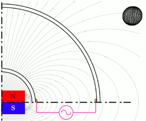
Figure 1. The spherical coordinate system we use is shown. Both spheres are set at rest. An electrolytic solution fills the gap between the outer and the inner spheres of radii  $a$ and
  $b$, respectively. The inner sphere encloses a permanent magnet, which produces the imposed dipolar magnetic field
  $\boldsymbol {B}^{0}$. The time-dependent electric current
  $\boldsymbol {j}^{0}$ is injected through two cooper rings located at the equators of the spheres, and the main direction of the Lorentz force is denoted by
  $\boldsymbol {F}^{0}$ which is also time dependent. (a) Sketch of the experimental device and (b) Meridional cut of the sketch.
Working with an aqueous solution may limit practical applications and experimental developments because the injection of an electric current unavoidably produces gas bubbles around the electrodes due to electrolysis. These bubbles disrupt the flow by modifying the electric current distribution, changing the boundary condition of the flow (Rivero & Cuevas Reference Rivero and Cuevas2012), occluding and interacting with the main flow and may oxidize the electrodes. These effects can be avoided or significantly reduced by two means: (i) in order to avoid disruption of the flow, several designs have been proposed to keep bubbles separated from the main region where main flow takes place (Rivero & Cuevas Reference Rivero and Cuevas2012, Reference Rivero and Cuevas2018), or (ii) using ac current (Lemoff & Lee Reference Lemoff and Lee2000). In the experiments reported in this manuscript, the ac frequencies and applied electric currents used show no effect of electrolysis on the flow of interest.
The dipolar magnetic field is generated by a rectangular parallelepiped Neodymium magnet with a side length of  $50.8$ mm, height of
  $25.4$ mm and maximum strength of
  $0.38$ T. The magnet is located in the centre inside the hollow inner sphere. The axis of the magnet is aligned with the vertical gravity vector. It is noteworthy to mention that it was found that the use of this magnet does not affect the symmetry of the flow. In fact, at the equatorial plane, which is where our work is focused, experimental measurements of the magnetic field, numerical simulations and the mathematical model (described in § 3) are in good agreement. The sinusoidal current is injected through the pair of electrodes and interacts with the non-uniform magnetic field distribution, generating an azimuthal Lorentz force that sets the fluid in motion. The ac electric current is obtained from a Stanford Research System DS345 function generator that produces a voltage of
  $\pm$20 V at frequencies in the range of 1
  $\mathrm {\mu }$Hz to 30.2 MHz with 1
  $\mathrm {\mu }$Hz frequency resolution. Three different frequencies were explored: 10, 50 and 100 mHz. The lower limit of this range has been selected as that is where distinguishable profiles are obtained, while the upper limit is determined in order to ensure the correct temporal resolution in accordance with the features of the camera (described below). Coincidentally, this range was found to be relevant for this study since a resonant behaviour and the decay of the boundary layer as a function of the forcing frequency were observed, as will be detailed in the following sections. The amplitude of the injected current was kept fixed to 50 mA (which corresponds to an electric current density of
  ${\approx }41$ A m
 $^{-2}$) with a serially connected potentiometer. With this value, laminar flow was explored, as will be shown in § 4. The electric signals were monitored with an oscilloscope and a digital multimeter, ensuring their oscillatory nature.
Since the electrolyte is a transparent medium, experimental velocity fields were obtained with PIV. A continuous 5 mW bright red (635 nm) laser module (Coherent Lasiris SNF Alignment and Structured Light Module) was placed in order to create a laser light plane parallel to the equator of the spheres. The light sheet was placed  $5$ mm above the equatorial plane and parallel to it, in order to avoid the electrodes, as shown in figure 1(b). The concentric spheres set-up was placed inside a rectangular container partially filled with water, the latter with the aim of reducing the aberration of the light sheet with the surface of the outer sphere. Flow images were extracted from video captured with a Nikon D80 camera with an AF micro-Nikkor
  $60$ mm f/2.8 D lens. The camera was supported on a holder
  $30$ cm below the experimental set-up. The actual area of the captured image was
  $14 \textrm {cm} \times 8 \textrm {cm}$. The images had
  $1280 \times 720$ pixel resolution. The time interval for the PIV measurements was
  $T/20$, where
  $T$ is the period of the forcing frequency. Avoiding transient flow, we obtained
  $40$ snapshots per cycle; the time interval between two subsequent images was
  $33$ ms. The relative phase of the forcing and observations was not experimentally recorded. Thus, for a given forcing frequency, numerical and theoretical results were shifted in order to minimize errors with experimental results. A minimum of ten cycles were averaged for the frequencies of
  $10$ and
  $50$ mHz, while only five cycles were averaged for the frequency of 100 mHz. The PIVlab software was used to perform the analysis (Thielicke & Stamhuis Reference Thielicke and Stamhuis2014); we used interrogation areas of
  $16 \times 16$ pixels with 50 % overlap in the horizontal and vertical directions, and vector validation. These conditions gave us a spatial resolution of
  $0.11\ \textrm {mm}\times 0.11\ \textrm {mm}$. Images were masked for the PIV analysis in order to perform the analysis only on the flow zone.
3. Theoretical model
It is important to remember that, in non-relativistic flows (such as those with electrolytes and liquid metals), charge density and displacement currents play no significant role, and therefore are disregarded (Davidson Reference Davidson2001). Thus for MHD flows, the two variables of interest are the fluid velocity and magnetic field. In the most general case, fluid velocity and magnetic field are coupled, but for experiments at the laboratory scale the problem can be simplified due to the low magnetic Reynolds number or quasi-static approximation. The magnetic Reynolds number is defined as  $R_{m} = U_c \ell \mu _0 \sigma$ where,
  $U_c$ and
  $\ell$ are the characteristic velocity and length, while
  $\mu _0$ is the magnetic permeability of vacuum and
  $\sigma$ the electrical conductivity of the medium. It can be interpreted as the ratio of advection to diffusion of the magnetic field. At the limiting case where
  $R_m {{\rightarrow 0}}$, magnetic diffusion dominates, and thus the fluid motion has no effect on the magnetic field, that is, the Navier–Stokes equations can be decoupled from the magnetic diffusion equation, which significantly reduces the complexity of the problem. For most of the experiments performed on Earth, such as that presented in this work, the magnitude of
  $R_m \ll 1$ and the low-
 $R_m$ approximation is valid. For the present experiment, this can be corroborated if we take
  $\ell = 0.067$ m (gap between spheres) while
  $U_c$ can be estimated from the balance between the inertial and Lorentz force terms, namely,
  $U_c \sim ( \ell j_0 B_0/\rho )^{1/2}$, with
  $j_0$ and
  $B_0$ the applied electric current density and the external magnetic field (0.065 T), respectively. Substitution of the corresponding values leads to
  $U_c= 0.01$ m s
 $^{-1}$, and thus
  $R_m = 5.35 \times 10^{-9}$. This means that the induced magnetic field is nine orders of magnitude smaller that the applied magnetic field. In turn, the induced magnetic field
  $b_0$ owing to the injected electric current
  $j_0$ can be estimated from Ampére's law as
  $b_0 \sim L_0 \mu _0 j_0$, which represents a factor of
  $5.3 \times 10^{-5}$ with respect to the applied magnetic field, and thus the total magnetic field can be taken as the applied one. In turn, the induced electric current is given by Ampére's law can be expressed in dimensionless form as
 \begin{equation} N \nabla^{*} \times \boldsymbol{b}^{*} = \boldsymbol{j}_i^{*}, \end{equation}
where the following dimensionless variables have been used  $\boldsymbol {r}^{*} = \boldsymbol {r}/d$,
  $\boldsymbol {j}_i^{*} = \boldsymbol {j}_i / j_0$ and
  $\boldsymbol {b}^{*} = \boldsymbol {b} / ( R_m B_{0} )$, with
  $\boldsymbol {b}$ the induced magnetic field,
  $d$ the gap between the spheres and
  $j_0$ the externally applied electric current. In this expression,
  $N$ corresponds to the magnetic interaction parameter (also referred to as the Stuart number) defined in terms of the Hartmann number
  $Ha$ and the Reynolds number
  $Re$ as
 \begin{equation} N = \frac{Ha^{2}}{Re} = \frac{B_0^{2} d^{2} \dfrac{\sigma}{\rho \nu}}{\dfrac{U_0 d}{\nu}} = \frac{\sigma d B_0^{2}}{\rho U_0}. \end{equation}
 Based on this definition, the magnetic interaction parameter corresponds to the ratio of electromagnetic to inertial forces, and thus is a measure of the influence of the magnetic field on the fluid flow. Based on the characteristic values in this work,  $Ha ^{2} = 0.11$ and
  $30 < {Re} < 723$, which lead to
  $1.5\times 10^{-4} < N < 3.7\times 10^{-3}$. From the dimensionless form of Ampere's law, it can be observed that
  $j_i \sim \mathcal {O} ( N )$. On the other hand, in dimensionless form, the applied electric current
  $\boldsymbol {j}_0$ is of order
  $\mathcal {O} ( 1 )$. Thus, the total electric current in dimensionless form can be written as
  $\boldsymbol {j}_T^{*} = \boldsymbol {j}_0^{*} + \boldsymbol {j}_i^{*}$, which for our experiments allows us to express the total electric current just as the externally applied electric current. In fact, flows driven by Lorentz forces created by the interaction of injected electric currents with applied magnetic fields in weak electrolytic solutions have been successfully modelled by neglecting induced effects for quasi-two-dimensional (Figueroa et al. Reference Figueroa, Demiaux, Cuevas and Ramos2009, Reference Figueroa, Meunier, Cuevas, Villermaux and Ramos2014) and three-dimensional models (Figueroa, Cuevas & Ramos Reference Figueroa, Cuevas and Ramos2011). This means that currents induced by the motion of the fluid in the magnetic field, as well as Lorentz forces produced by these currents, can be completely disregarded. In this case, the flow is governed by the continuity equation and the Navier–Stokes equation with the Lorentz force term (only the product of the applied electric current and external magnetic field). In dimensionless terms the governing equations read
 $$\begin{gather} \boldsymbol{\nabla} \boldsymbol{\cdot}\boldsymbol{u}=0, \end{gather}$$
 $$\begin{gather}{Re}_{\omega} \frac{\partial \boldsymbol{u}}{\partial t} + (\boldsymbol{u} \boldsymbol{\cdot} \boldsymbol{\nabla}) \boldsymbol{u} ={-}\boldsymbol{\nabla} p + \nabla^{2} \boldsymbol{u} + Q\,\boldsymbol{j}^{0} \times \boldsymbol{B}^{0}, \end{gather}$$
where  $\boldsymbol {u}$ stands for the velocity vector, normalized by
  $u_0=\nu /d$,
  $\nu$ and
  $d$ being the kinematic viscosity of the fluid and the characteristic length, namely, the gap between spheres
  $d=a-b$. The pressure field is denoted by
  $p$, normalized by
  $\rho u_0^{2}$, where
  $\rho$ is the density of the fluid. Coordinates are normalized by
  $d$. In turn, time
  $t$ is normalized with the angular frequency of the forcing
  $\omega =2{\rm \pi} f$, where
  $f$ is the ordinary frequency of the ac current. The last term on the right-hand side of (3.4) represents the oscillating Lorentz force created by the non-uniform magnetic field distribution
  $\boldsymbol {B}^{0}$ normalized by the amplitude of the magnetic field at the equator of the inner sphere
  $B^{0}= 0.065$ T, and the time-dependent applied electric current
  $\boldsymbol {j}^{0}$, which is normalized by the current amplitude
  $j^{0}$. The flow is governed by the flow parameter
  $Q=U_0 /u_0$, that compares two velocity scales: the scale defined from the balance between the Lorentz and viscous forces
  $U_0= j^{0} B^{0} d^{2}/\rho \nu$ (Figueroa et al. Reference Figueroa, Demiaux, Cuevas and Ramos2009) and the viscous velocity scale
  $u_0=\nu / d$. In fact, the parameter
  $Q$ can be interpreted as the ratio of the electromagnetic and mechanical energies. Considering that (3.4) was obtained under the low-
 $R_m$ approximation, it is possible to estimate an upper limit for the parameter
  $Q$ in the actual experiment, above which modifications to the governing equations are required. It seems plausible to consider that
  $R_m \sim 0.01$ satisfies the low-
 $R_m$ approximation, allowing us to estimate a value for the injected current that would induce a magnetic field
  $b_0 \sim 0.01 B^{0}$. From Ampére's law, this injected current is found to be
  $j_0 \sim 7720$ A m
 $^{-2}$, which means that theoretically
  $Q \leq 3 \times 10^{10}$. Nevertheless, it is important to point out that, even when analytical solutions exist, this does not imply that those solutions are stable through all of the range, but this analysis is not within the scope of this work. The oscillatory Reynolds number is defined as
  ${Re}_{\omega }=\omega d^{2} / \nu$. For the explored frequency range, and considering the corresponding characteristic scales, the oscillatory Reynolds number explored experimentally is in the range
  $28 < {Re}_{\omega } < 2820$. The system of (3.3) and (3.4) is fully determined, providing the injected current
  $\boldsymbol {j}^{0}$ and the applied magnetic field
  $\boldsymbol {B}^{0}$. In dimensionless terms, the applied magnetic field is denoted as
 \begin{equation} \boldsymbol{B}^{0} = \frac{b^{3}}{r^{3}} \left( 2 \cos \phi \hat{r} + \sin \phi \hat{\phi} \right),\end{equation}
where  $\phi$ is the colatitude,
  $\hat {r}$ and
  $\hat {\phi }$ are the unitary vectors in the radial and polar directions and
  $b$ is the dimensionless radius of the inner sphere. The expression for the current density comes from Ohm's law for weakly conducting fluids, which in dimensionless terms reads
 \begin{equation} \boldsymbol{j} = \boldsymbol{\nabla} \varphi, \end{equation}
where  $\varphi$ is the electric potential. Considering an electrolyte as the working fluid, that is, the induced effects are neglected, and there is charge conservation
  $\boldsymbol {\nabla }\boldsymbol {\cdot } \boldsymbol {j}=0$, the electric potential
  $\varphi$ obeys a Laplacian equation, that is
 \begin{equation} \nabla^{2} \varphi = 0. \end{equation}
 Assuming that both spheres act as perfect electrical conductors, that is perfect conductive shells  $( 0 \leq \phi \leq {\rm \pi}\textrm { and } 0\leq \theta \leq 2 {\rm \pi})$, the electric potential is only
  $r$-dependent. Considering time-dependent Dirichlet boundary condition at the inner sphere
  $\varphi ( b )=\sin ( t )$ and fixed at the outer sphere
  $\varphi ( a ) = 0$, leads us to the following solution:
 \begin{equation} \varphi \left( r,t \right) = \frac{ b \left( a-r \right) }{r \left( a-b \right) } \sin \left( t \right). \end{equation}
 The electric current density  $j_r$ can be obtained from Ohm's law, (3.6)
 \begin{equation} j_r \left( r,t \right) = \frac{ab}{ \left( a-b \right) r^{2}} \sin \left( t \right). \end{equation}
 Analogously, the radial electric current density for the case of ring electrodes located at the equator  $( \phi ={\rm \pi} /2 \textrm { and } 0\leq \theta \leq 2 {\rm \pi})$, as in Figueroa et al. (Reference Figueroa, Rojas, Rosales and Vázquez2016), is found to be
 \begin{equation} j_r \left( r,t \right) = \frac{b^{2}}{r^{2}} \sin \left( t \right). \end{equation}
For this case, it must be mentioned that the solution of (3.7) implies the existence of a current density component in the polar direction. It is important to highlight two facts. Firstly, considering the most general case where the external magnetic field and applied electric current have components only in the radial and polar coordinates leads to a Lorentz force with only one component in the azimuthal direction with at most two terms. Since the polar component of the current and the radial component of the magnetic field vanish at the equator, only one term remains in this plane. Secondly, derived from the previous point and considering that both spheres remain static, in the laminar regime the resulting movement is such that a particle will follow a closed circular motion within its plane and parallel to the equator.
It can be observed that, in both (3.9) and (3.10), the electric current density is in the form of  $r^{-2}$. The system of (3.3) and (3.4) along with the expression for the magnetic field, (3.5), and the current density (3.9) or (3.10) form a closed system for solving the electromagnetically driven flow in the gap between the spheres.
3.1. Analytical solutions
As described in previous sections, the main aim of this work is to find a solution that can be compared against experimental measurements performed at the equatorial plane. In order to do this, only the existence of the azimuthal velocity component will be assumed, which has a radial and temporal dependence, namely  $\boldsymbol {u} = [ 0,0,u_{\theta } (r,t ) ]$. In addition, there is no imposed pressure gradient in the azimuthal direction in such way that, at most,
  $p = p ( r,\phi )$. Now, the interaction of the external magnetic field (with components in the
  $r$ and
  $\phi$ directions) and the radially injected electric current produces a Lorentz force with a unique component in the azimuthal direction. Under these assumptions, the continuity equation is satisfied identically. In turn, the equation for the velocity component in the radial direction establishes a balance between the centrifugal force and the pressure gradient in the radial direction that counteracts it. For the equation of the velocity component in the polar direction
  $\phi$, a pressure gradient in the polar direction is assumed, which balances the remaining inertial term whose dependence is also in this direction. Finally, for the azimuthal direction, the inertial terms vanish and a viscous term appears which depends on the azimuthal Lorentz force, as well as on the polar coordinate as
  $\sin ^{-2}\theta$.
Let us address the problem in a very simplified way that allows us to obtain some analytic solutions for the flow at the equatorial plane. In this plane,  $\phi ={\rm \pi} /2$,
  $u_{\theta }$ no longer depends on
  $\phi$ (since
  $\sin ^{-2} \phi = 1$), yielding a component that only depends on the
  $r-$direction, leading to an axisymmetric flow. In this symmetry plane, the electric currents point in the radial direction, while the magnetic field points in the vertical direction (as observed in figure 1). Under these assumptions, the set of (3.3)–(3.4) reduces to
 \begin{equation} {Re} _{\omega} \frac{\partial u_\theta}{\partial t} = \frac{\partial^{2} u_\theta}{\partial r^{2}} + \frac{2}{r} \frac{\partial u_\theta}{\partial r} - \frac{u_\theta}{r^{2}} - Q \frac{ab^{4}}{(a-b)r^{5}} \sin t. \end{equation}
 The last term on the right-hand side of (3.11) corresponds to the applied Lorentz force when both spheres are conducting shells, that is, the electric current comes from (3.9). We must note that the electromagnetic dependence in the  $r$-direction decays as
  $r^{-5}$. Neglecting the transient flow, and considering that
 \begin{equation} u_{\theta} \left( r , t \right) = \mbox{Im} \left[ f \left( r \right) \mathrm{e}^{\textrm{i} t} \right], \end{equation}
where  $\mbox {Im}$ indicates the imaginary part inside the brackets, the following expression for
  $f ( r )$
 \begin{equation} \frac{{\textrm{d}}^{2} f \left( r \right)}{{\textrm{d}}r^{2}} + \frac{2}{r} \frac{{\textrm{d}}f \left( r \right)}{{\textrm{d}}r} - f \left( r \right) \left( \frac{1}{r^{2}} + \textrm{i} {Re}_{\omega} \right) = \frac{A}{r^{5}}, \end{equation}
is obtained, where  $A=Q ab^{4}/ ( a-b )$. Since the velocity satisfies the no-slip condition on both radii, the boundary conditions for
  $f$ lead to
  $f ( b ) = f ( a ) = 0$.
3.1.1. Asymptotic and approximate solutions
Equation (3.13) corresponds to the inhomogeneous spherical Bessel function of irrational order, which is not easy to solve, as will be seen in § 3.1.2. However, if we take the limiting case  ${Re}_{\omega } {{\rightarrow 0}}$, it gets easier and we are able to find an asymptotic solution. In this limiting case, (3.13) reduces to
 \begin{equation} \frac{{\textrm{d}}^{2} f \left( r \right)}{{\textrm{d}}r^{2}} + \frac{2}{r} \frac{{\textrm{d}}f \left( r \right)}{{\textrm{d}}r} - \frac{f \left( r \right)}{r^{2}} = \frac{A}{r^{5}}. \end{equation}
 For (3.14), the homogeneous part is a second-order Euler equation, which can be easily solved. The solution to the inhomogeneous equation can be obtained by the variation of parameters method. The asymptotic solution to the low  ${Re} _{\omega }$ approximation is found to be
 \begin{align} u_\theta(r,t) ={-} \frac{ A \sin \left( t \right) }{5 \left( a^{\sqrt{5}} - b^{\sqrt{5}} \right) r^{3}} \left[ b^{\sqrt{5}} - b^{l} r^{m} + a^{l} r^{{-}l} \left( r^{\sqrt{5}} - b^{\sqrt{5}} \right) + a^{\sqrt{5}} \left( b^{l} r^{{-}l} - 1 \right) \right], \end{align}
where the superscript indices are  $l=1/2 ( \sqrt {5} - 5 )$ and
  $m=1/2 ( 5 + \sqrt {5} )$. It is important to note that this expression has real arguments. If we try to find an asymptotic solution for the opposite case,
  ${Re}_{\omega } \to \infty$, this leads to a particular solution which cannot be expressed easily. As a first approach, and in order to find an approximate solution, we assume that
  $r^{-2} \ll \textrm {i} Re_{\omega }$ in the third term of the left-hand side of (3.13), which leads to
 \begin{equation} \frac{{\textrm{d}}^{2} f \left( r \right)}{{\textrm{d}}r^{2}} + \frac{2}{r} \frac{{\textrm{d}}f \left( r \right)}{{\textrm{d}}r} - \textrm{i} {Re}_{\omega} f \left( r \right) = \frac{A}{r^{5}}. \end{equation}
 Expressed in terms of the exponential integral function  $Ei$, the approximate solution of (3.16) is
 \begin{align} u_{\theta} \left( r , t
\right) &= \mbox{Im}\ \left\lbrace\textrm{e}^{\textrm{i}t}
\cdot \frac{A \ \textrm{e}^{-\zeta r}}{12 a^{2} b^{2} r^{3}
\left( \textrm{e} ^{2 a \zeta} - \textrm{e} ^{2 b \zeta}
\right)} \left\lbrace\vphantom{\left\lbrace \left[
\textrm{e} ^{2 \left( a + b \right) \zeta} - \textrm{e} ^{2
\left( a + r\right) \zeta} \right] Ei \left( - a \zeta
\right) + \left[ \textrm{e} ^{2 b \zeta} - \textrm{e} ^{2 r
\zeta} \right] Ei \left( a \zeta \right) \right.} 2 \left[
b^{2} r^{2} \left( \textrm{e} ^{\left( a + 2b\right) \zeta}
- \textrm{e} ^{\left( a + 2r\right) \zeta} \right) \right.
\right. \right. \nonumber\\ &\quad + \left. \left. \left. a^{2}
\left[ b^{2} \left( \textrm{e} ^{\left( 2a + r\right)
\zeta} - \textrm{e} ^{ \left( 2b + r \right) \zeta} \right)
- r^{2} \left( \textrm{e} ^{\left( 2a + b\right) \zeta} -
\textrm{e} ^{\left( 2r + b \right) \zeta} \right) \right]
\right]\vphantom{\left\lbrace \left[ \textrm{e} ^{2 \left(
a + b \right) \zeta} - \textrm{e} ^{2 \left( a + r\right)
\zeta} \right] Ei \left( - a \zeta \right) + \left[
\textrm{e} ^{2 b \zeta} - \textrm{e} ^{2 r \zeta} \right]
Ei \left( a \zeta \right) \right.}\right.\right.\nonumber\\
&\quad - \left. \left. \textrm{i} a^{2} b^{2} {Re} _{\omega}
r^{2} \left\lbrace \left[ \textrm{e} ^{2 \left( a + b
\right) \zeta} - \textrm{e} ^{2 \left( a + r\right) \zeta}
\right] Ei \left( - a \zeta \right) + \left[ \textrm{e} ^{2
b \zeta} - \textrm{e} ^{2 r \zeta} \right] Ei \left( a
\zeta \right) \right.\right.\right. \nonumber\\ &\quad - \left.\left.\left.\textrm{e} ^{2
\left( a +b \right) \zeta} Ei \left({-}b \zeta \right) +
\left[ \textrm{e} ^{2 r \zeta} - \textrm{e} ^{2 a \zeta}
\right] Ei \left( b \zeta \right) \right.\right.\right.\nonumber\\ &\quad
+ \left.\left.\left. \textrm{e} ^{2 \left( b + r \right) \zeta} \left[ Ei
\left({-}b \zeta \right) - Ei \left({-}r \zeta \right)
\right] \right.\right.\right.\nonumber\\ &\quad + \left.\left.\left.\textrm{e} ^{2 \left( a + r \right)
\zeta} Ei \left({-}r \zeta \right) + \textrm{e} ^{2 a
\zeta} Ei \left( r \zeta \right) - \textrm{e} ^{2 b \zeta}
Ei \left( r \zeta \right)\right\rbrace \right\rbrace \vphantom{\frac{A \
\textrm{e}^{-\zeta r}}{12 a^{2} b^{2} r^{3} \left(
\textrm{e} ^{2 a \zeta} - \textrm{e} ^{2 b \zeta} \right)}
}\right\rbrace, \end{align}
\begin{align} u_{\theta} \left( r , t
\right) &= \mbox{Im}\ \left\lbrace\textrm{e}^{\textrm{i}t}
\cdot \frac{A \ \textrm{e}^{-\zeta r}}{12 a^{2} b^{2} r^{3}
\left( \textrm{e} ^{2 a \zeta} - \textrm{e} ^{2 b \zeta}
\right)} \left\lbrace\vphantom{\left\lbrace \left[
\textrm{e} ^{2 \left( a + b \right) \zeta} - \textrm{e} ^{2
\left( a + r\right) \zeta} \right] Ei \left( - a \zeta
\right) + \left[ \textrm{e} ^{2 b \zeta} - \textrm{e} ^{2 r
\zeta} \right] Ei \left( a \zeta \right) \right.} 2 \left[
b^{2} r^{2} \left( \textrm{e} ^{\left( a + 2b\right) \zeta}
- \textrm{e} ^{\left( a + 2r\right) \zeta} \right) \right.
\right. \right. \nonumber\\ &\quad + \left. \left. \left. a^{2}
\left[ b^{2} \left( \textrm{e} ^{\left( 2a + r\right)
\zeta} - \textrm{e} ^{ \left( 2b + r \right) \zeta} \right)
- r^{2} \left( \textrm{e} ^{\left( 2a + b\right) \zeta} -
\textrm{e} ^{\left( 2r + b \right) \zeta} \right) \right]
\right]\vphantom{\left\lbrace \left[ \textrm{e} ^{2 \left(
a + b \right) \zeta} - \textrm{e} ^{2 \left( a + r\right)
\zeta} \right] Ei \left( - a \zeta \right) + \left[
\textrm{e} ^{2 b \zeta} - \textrm{e} ^{2 r \zeta} \right]
Ei \left( a \zeta \right) \right.}\right.\right.\nonumber\\
&\quad - \left. \left. \textrm{i} a^{2} b^{2} {Re} _{\omega}
r^{2} \left\lbrace \left[ \textrm{e} ^{2 \left( a + b
\right) \zeta} - \textrm{e} ^{2 \left( a + r\right) \zeta}
\right] Ei \left( - a \zeta \right) + \left[ \textrm{e} ^{2
b \zeta} - \textrm{e} ^{2 r \zeta} \right] Ei \left( a
\zeta \right) \right.\right.\right. \nonumber\\ &\quad - \left.\left.\left.\textrm{e} ^{2
\left( a +b \right) \zeta} Ei \left({-}b \zeta \right) +
\left[ \textrm{e} ^{2 r \zeta} - \textrm{e} ^{2 a \zeta}
\right] Ei \left( b \zeta \right) \right.\right.\right.\nonumber\\ &\quad
+ \left.\left.\left. \textrm{e} ^{2 \left( b + r \right) \zeta} \left[ Ei
\left({-}b \zeta \right) - Ei \left({-}r \zeta \right)
\right] \right.\right.\right.\nonumber\\ &\quad + \left.\left.\left.\textrm{e} ^{2 \left( a + r \right)
\zeta} Ei \left({-}r \zeta \right) + \textrm{e} ^{2 a
\zeta} Ei \left( r \zeta \right) - \textrm{e} ^{2 b \zeta}
Ei \left( r \zeta \right)\right\rbrace \right\rbrace \vphantom{\frac{A \
\textrm{e}^{-\zeta r}}{12 a^{2} b^{2} r^{3} \left(
\textrm{e} ^{2 a \zeta} - \textrm{e} ^{2 b \zeta} \right)}
}\right\rbrace, \end{align}
where  $\zeta = \sqrt {\textrm {i} {Re} _{\omega }}$. It should be noted that this approximate solution (3.17) is expressed in terms of complex arguments (see the definition of
  $\zeta$), and the imaginary part must be taken as the approximate solution for the velocity. So far, we have found an asymptotic solution for
  ${Re} _{\omega } {{\rightarrow 0}}$ and an approximate solution for
  ${Re} _{\omega } \to \infty$. Now we turn our attention to trying to find the full solution of (3.11) in terms of real arguments, which is described in the following subsection.
3.1.2. Exact solution
As stated previously, the analytical solution of (3.11) is obtained by considering (3.12), which leads to (3.13), and whose solution can be written as
 \begin{equation} f \left( r \right)= C_1 y_1 \left( r \right) + C_2 y_2 \left( r \right) + y_P \left( r \right), \end{equation}
where subindex  $P$ refers to the particular solution, and
  $y_1$ and
  $y_2$ are the solutions of the homogeneous equation. In order to find a solution in terms of real arguments, we expand
  $f ( r )$ in its real,
  $_R$, and imaginary,
  $_I$, parts
 \begin{align} f \left( r \right) &= \left( C_{1R} + \textrm{i} C_{1I} \right) \left[ y_{1R} \left( r \right) + \textrm{i} y_{1I} \left( r \right) \right] \nonumber\\ &\quad + \left( C_{2R} + \textrm{i} C_{2I} \right) \left[ y_{2R} \left( r \right) + \textrm{i} y_{2I} \left( r \right) \right] \nonumber\\ &\quad + y_{PR} \left( r \right) + \textrm{i} y_{PI} \left(r\right). \end{align}
Therefore,  $f(r)$ can be expressed in terms of real and imaginary components
 \begin{equation} f \left( r \right)=y_R \left( r \right) + \textrm{i} y_I \left( r \right). \end{equation}
Real and complex solutions of the homogeneous equation were obtained by substituting the complex expression and getting a fourth-order ordinary differential equation. The particular solution was obtained by the variation of parameters method, whereas the constants were obtained from boundary conditions. From (3.12) and (3.20) it can be seen that
 \begin{equation} u_{\theta} \left( r , t \right) = y_I \left( r \right) \cos \left( t \right) + y_R \left( r \right) \sin \left( t \right), \end{equation}
where
 \begin{align} y_R \left( r \right) &={-}C_{1I} y_{1I} \left( r \right) + C_{1R} y_{1R} \left( r \right) \nonumber\\ &\quad - C_{2I} y_{2I} \left( r \right) + C_{2R} y_{2R} \left( r \right) + y_{PR} \left(r\right), \end{align}
 \begin{align} y_I \left( r \right) &= C_{1R} y_{1I} \left( r \right) + C_{1I} y_{1R} \left( r \right) \nonumber\\ &\quad + C_{2R} y_{2I} \left( r \right) + C_{2I} y_{2R} \left( r \right) + y_{PI} \left(r\right). \end{align}
The solutions to the homogeneous part of (3.13) are
 \begin{equation} \left.\begin{gathered} y_{1R} \left( r \right) ={+} r^{-({1}/{2})} {bei}_{{5}/{2}} \left( \sqrt{{Re} _{\omega}} r \right),\\ y_{1I} \left( r \right) ={-} r^{-({1}/{2})} {ber}_{{5}/{2}} \left( \sqrt{{Re} _{\omega}} r \right), \\ y_{2R} \left( r \right) ={+} r^{-({1}/{2})} {kei}_{{5}/{2}} \left( \sqrt{{Re} _{\omega}} r \right), \\ y_{2I} \left( r \right) ={-} r^{-({1}/{2})} {ker}_{{5}/{2}} \left( \sqrt{{Re} _{\omega}} r \right), \end{gathered}\right\} \end{equation}
where  ${bei}$,
  ${ber}$,
  ${kei}$ and
  ${ker}$ are the Kelvin functions. In turn, the real and imaginary solutions of the particular equation are given in Appendix A. This allows us to express the real and imaginary parts of the particular solution as
 $$\begin{gather} y_{PR} \left(r\right) ={-}y_{P1I} \left(r\right) y_{1I} \left( r \right) + y_{P1R} \left(r\right) y_{1R} \left( r \right) - y_{P2I} \left(r\right) y_{2I} \left( r \right) + y_{P2R} \left(r\right) y_{2R} \left( r \right), \end{gather}$$
 $$\begin{gather}y_{PI} \left(r\right) = y_{P1R} \left(r\right) y_{1I} \left( r \right) + y_{P1I} \left(r\right) y_{1R} \left( r \right) + y_{P2R} \left(r\right) y_{2I} \left( r \right) + y_{P2I} \left(r\right) y_{2R} \left( r \right). \end{gather}$$
 It is now possible to obtain the coefficients of (3.22). For the sake of clarity, the coefficients  $C_{1R}$,
  $C_{1I}$,
  $C_{2R}$ and
  $C_{2I}$ are presented in Appendix B. Even though the analytical solutions obtained are based on strong assumptions, they are helpful for the physical understanding of the flow, as will be shown in § 4.
In order to test the validity of the approximate solutions (3.15) and (3.17), they are compared against the exact solution (3.21). This comparison is done in terms of the squared deviation between the two functions  $F_1$ and
  $F_2$ on
  $[ b,a]$ defined as
 \begin{equation} \epsilon^{2}= \frac{\displaystyle\int_b^{a} \vert F_1 \left( x \right) - F_2 \left( x \right) \vert ^{2} \,{\textrm{d}\kern0.06em x} }{\displaystyle\int_b^{a} \vert F_1 \left( x \right) \vert ^{2} \,{\textrm{d}\kern0.06em x}}, \end{equation}
where  $F_1$ corresponds to the exact solution, and
  $F_2$ is the corresponding asymptotic or approximate solution. Figure 2 shows the squared deviation between the exact and the asymptotic or approximate solutions as a function of the oscillatory Reynolds number within the ranges of interest. Based on this criterion, considering a squared deviation of
  $10^{-2}$ shows that the upper and lower limits for the low-
 ${Re} _{\omega }$ asymptotic solution and the high-
 ${Re} _{\omega }$ approximations are
  ${Re} _{\omega } \sim 1$, respectively. If
  $\epsilon ^{2} = 10^{-3}$, then these limits are
  ${Re} _{\omega } \leq 0.3$ for the low-
 ${Re} _{\omega }$ asymptotic solution and
  ${Re} _{\omega } \geq 50$ for the high-
 ${Re} _{\omega }$ approximations. The radial profiles of the azimuthal velocity
  $u_{\theta }$ at the equatorial plane for the approximate and exact solutions are compared in figure 3 at different phases
  $\alpha$ of the oscillation. Within the validity ranges of each approximate solution (continuous lines), the profiles overlap on the exact solution (dashed lines).

Figure 2. Squared deviation between exact and approximate solutions as a function of the oscillatory Reynolds number within the ranges of interest.

Figure 3. Radial profiles of azimuthal velocity  $u_{\theta }$ at the equatorial plane with
  $Q=1$ for different phases
  $\alpha$ for (a)
  ${Re} _{\omega }=1$ and (b)
  ${Re} _{\omega }=100$. Red lines and dots denote
  $\alpha =1/6 {\rm \pi}$ and
  $\alpha =7/6 {\rm \pi}$. Green lines and crosses correspond to
  $\alpha =1/3 {\rm \pi}$ and
  $\alpha =4/3 {\rm \pi}$. For blue lines and circles,
  $\alpha =1/2 {\rm \pi}$ and
  $\alpha =3/2 {\rm \pi}$. Dashed lines: exact analytical solution, (3.21). Continuous lines in (a) show the low
  ${Re} _{\omega }$ approximation, (3.15), and in (b) the high
  ${Re} _{\omega }$ approximation, (3.17). Markers: numerical calculations.
3.2. Numerical solution
The one-dimensional analytical solutions obtained in the last subsection approximate the velocity profiles at the equatorial plane and, as discussed in the previous section, do not take into account convective effects. In general, convective effects may promote the three-dimensionality of the flow and therefore, an accurate modelling requires a three-dimensional (3-D) numerical approach. In order to get the complete velocity field at different locations of the flow region, the system of (3.3) and (3.4) was solved numerically. An in-house code using the finite difference method based on the procedure described in Griebel, Dornseifer & Neunhoeffer (Reference Griebel, Dornseifer and Neunhoeffer1998) and Cuevas, Smolentsev & Abdou (Reference Cuevas, Smolentsev and Abdou2006) was adapted to the spherical coordinate system, including electromagnetic forces. In the experiment, the inner sphere is held by a glass shaft, which was not included in the numerical model. The calculation of the time-dependent Lorentz force term in (3.4) requires the full 3-D magnetic field distribution of the permanent magnet (3.5) and the radially injected electric current at the equator (3.9) or (3.10). For this latter case, the number of elements in the polar direction was adjusted to better fit the heights of the inner and outer electrodes. Namely, ring electrodes are modelled as surfaces, not as a line source at the equator. The numerical model uses a uniform staggered mesh and, although there exists a small difference between the inner and outer electrode heights, no significant changes were observed in the obtained results. The applied electric current  $j_r$ is calculated from (3.9). Note that the electric current is only computed in cells that span radially from the inner to the outer electrode, otherwise it vanishes. The numerical solution considers no-slip conditions on the spheres. The initial boundary conditions refer to a quiescent fluid (
 $\boldsymbol {u}=0$) with no electric potential gradient (or
  $\boldsymbol {j}=0$). In the calculations, a time step of 2
 $\times 10^{-7}$
  $T_{\omega }$ was used, where
  $T_{\omega }=2 {\rm \pi}$ which is the dimensionless the period of the oscillation of the applied Lorentz force, along with a spatial resolution of
  $480 \times 30 \times 60$ in the
  $r$,
$r$,  $\theta$ and
  $\phi$ directions, respectively.
The numerical code has been successfully compared to experimental results where the flow is promoted due to the rotation of the inner sphere (Wimmer Reference Wimmer1976) and due to a Lorentz force that is constant in time (Figueroa et al. Reference Figueroa, Rojas, Rosales and Vázquez2016). Moreover, considering (3.9) for the applied current, the code is compared quantitatively to the analytical solutions, as seen in figure 3. In the latter, azimuthal velocity  $u_{\theta }$ profiles as a function of the
  $r$ coordinate for different phases
  $\alpha$ are shown. We can observe that, in the creeping flow regime (
 $Q=1$), the numerical results (markers) agree quantitatively with the analytical solutions (lines) for small and high
  ${Re}_{\omega }$. An important feature in the results is the reduction in magnitude of the velocity and the boundary layer width by increasing
  ${Re}_{\omega }$. This point will be addressed in the next section. The comparison shown in figure 3 validates the numerical code and the assumptions made for the analytical solutions. In the next section, numerical results are successfully compared to experimental measurements. For this case, the numerical simulation was run in a volume that corresponds to the dimensions of the experimental set-up and considered (3.10) for the applied electric current density.
4. Results
When the radially injected electric current interacts with the dipolar magnetic field, a Lorentz force, which mainly points in the  $\theta$-direction, is generated. The electromagnetic force drives a rotational flow in the gap between the spheres. Since the electric current obeys a sinusoidal function, the electric signal will behave accordingly, making the flow change its direction of rotation and oscillate in time. In order to visualize how the azimuthal velocity diffused towards the poles for different forcing frequencies, the numerical results for
  $u_{\theta }$ in the meridional plane at a given oscillation phase
  $\alpha$ are shown in figure 4. In all numerical simulations the magnitude of the electric current was kept constant. The amplitude of the injected electric current was
  $I=50$ mA, which corresponds to a flow parameter of
  $Q=7.35 \times 10^{5}$. For the low forcing frequency
  ${Re}_{\omega }=28$, see figure 4(a). The velocity is intense in the equatorial zone close to the inner sphere. The flow interacts with the outer sphere and, due to its intensity, it reaches the polar zone of the outer sphere. When the forcing frequency is increased (
 ${Re}_{\omega }=282$), as seen in figure 4(b), the flow does not reach the polar zone and is reduced to the equatorial zone and alternating positive and negative values are observed in the polar direction as the flow oscillates. Further increasing the forcing frequency (
 ${Re}_{\omega }>2820$), the flow is visible closer to the inner sphere's equatorial zone and the intensity of the velocity is decreased, see figures 4(c) and 4(d).

Figure 4. Contour map of azimuthal velocity  $u_{\theta }$ at the meridional plane from numerical simulations: (a)
  $\alpha =10/6 {\rm \pi}$,
  $f=1$ mHz (
 ${Re}_{\omega }=28$); (b)
  $\alpha =11/6 {\rm \pi}$,
  $f=10$ mHz (
 ${Re}_{\omega }=282$; (c)
  $\alpha =0$,
  $f=100$ (
 ${Re}_{\omega }=2820$); (d)
  $\alpha =0$,
  $f=1000$ mHz (
 ${Re}_{\omega }=28\,205$). Electric current
  $I=50$ mA
  $(Q=7.35 \times 10^{5})$.
Figure 5 shows the experimental (a,c,e) and numerical (b,d, f) profiles of the azimuthal velocity  $u_{\theta }$ located at the equatorial line between the concentric spheres system. The radial profiles are drawn for different time instants in order to visualize the dynamics of the flow. Experimental profiles are presented from raw data and thus, given the spatio-temporal resolution of the PIV system, some fluctuations are observed but do not correspond to turbulence in the flow. In fact, the flow is laminar within the explored experimental conditions. For
  ${Re} _{\omega } = 282$ and
  $140$, an asymmetry can be noted in the experimental profiles. Because the electrode is a physical impediment for the visualizations at the equatorial plane, the PIV measurements were obtained at approximately
  $4$ mm above the symmetry plane, and thus an asymmetry can be expected. We can observe that, for high forcing frequencies, the profiles resemble those observed in the Stokes second problem. However, for this electromagnetically driven flow, due to the stationary boundaries, the maximum velocity is located in the bulk of the flow. It can be observed that, as the frequency increases, the amplitude and penetration depth decrease. The Reynolds number based on the highest velocity for
  $f=10$ mHz
  $( u_{\theta , \max } = 9.6\ \textrm {mm}\ \textrm {s}^{-1})$ corresponds to
  ${Re} = u_{\theta , \max }\ d/\nu = 640$. From these plots, it can be noted that numerical simulations are in good qualitative and quantitative agreement with the experimental PIV measurements. If we compare these results with the analytical profiles in figure 3, we can deduce that the analytical results for low frequencies do not match the experimental observations since convective effects are noticeable, while results for high frequencies agree well qualitatively because diffusive effects are stronger.

Figure 5. Radial profiles of azimuthal velocity  $u_{\theta }$ at the equatorial plane. (a,c,e) Experimental measurements. (b,d,f) Numerical simulations. Panels (a,b)
  $f=10$ mHz (
 ${Re}_{\omega }=282$); (c,d)
  $f=50$ mHz (
 ${Re}_{\omega }=1410$); (e,f)
  $f=100$ mHz (
 ${Re}_{\omega }=2820$). Blue lines denote the phases
  $\alpha =1/6 {\rm \pi}$ and
  $\alpha =7/6 {\rm \pi}$. Green lines denote the phases
  $\alpha =2/6 {\rm \pi}$ and
  $\alpha =8/6 {\rm \pi}$. Red lines denote the phases
  $\alpha =6/6 {\rm \pi}$ and
  $\alpha =9/6 {\rm \pi}$. Electric current
  $I=50$ mA.
As previously discussed, as the forcing frequency increases, the magnitude of the highest velocity  $u_{\theta , max}$ diminishes, as seen in figure 6. It can be observed that the amplitude of the azimuthal velocity decays as
  ${Re} _{\omega }^{-1}$ asymptotically to zero, which is depicted as a dashed black line. The curve is also plotted for the Reynolds number
  ${Re}$ as a function of the oscillatory Reynolds number
  ${Re} _{\omega }$. Moreover, a maximum value for the amplitude is approximately
  $f = 20$ mHz (
 ${Re} _{\omega }=564$), that is, a resonant behaviour of the flow is found due to the time-dependent forcing. This phenomenon is currently under investigation.

Figure 6. Maximum amplitude of the velocity  $u_{\max }$ as a function of the forcing frequency
  $f$. The points represent numerical measurements, the line is plotted to guide the eye.
4.1. Boundary layer
This section describes the estimation of the thickness and shape of the boundary layer (BL) at the inner sphere, which is based on the exact solution presented in § 3.1.2. Although different analytical methods have been reported to estimate the BL, such as integrals or derivative-based methods (Rivero et al. Reference Rivero, Garzón, Núñez and Figueroa2019), their implementation for the analytical solution presented in this work (3.21) does not lead to simple expressions. Moreover, these formulations are valid only for semi-infinite problems, which is not the case here since the maximum value of the velocity is non-monotonic at the gap centre, that is, it is impossible to define an exact location at which the velocity profile reaches an asymptotic behaviour. From the analytical and numerical solutions, a BL can be observed close to the inner radius.
With the lack of an obvious method for defining the BL thickness, we defined an analogous method for the 99 % BL thickness. The BL thickness is the distance from the inner radius where
 \begin{equation} \frac{u_{\theta} \left( r , t \right)}{u_{\theta , \max} } = 10^{{-}1}. \end{equation}
The velocity is defined as
 \begin{equation} u_{\theta} \left( r , t \right) = y_R \left( r \right) \sin \left( t \right) +y_I \left( r \right) \cos \left( t \right), \end{equation}
which can be expressed as
 \begin{equation} u_{\theta} \left( r , t \right) = A \left(r \right) \sin \left( t + \psi \left( r \right) \right), \end{equation}
where  $A(r)$ corresponds to the amplitude and
  $\psi ( r )$ to the phase, given by
 \begin{equation} A \left(r \right) =\sqrt{y_R \left( r \right)^{2}+y_I \left( r \right)^{2}},\quad \sin \left( \psi \left( r \right) \right)=\frac{y_I \left( r \right)}{A \left( r \right)}. \end{equation}
 Since a characteristic flow velocity is unknown a priori, the maximum velocity is used as the reference velocity. In addition, noting that  $| \sin ( t+ \psi ( r ) )| \leq 1$, we estimate the BL thickness based only on the amplitude
  $A ( r )$ of the BL.
Figure 7 shows the amplitude and phase shift of the velocity as functions of the oscillatory Reynolds number (for  ${Re}_{\omega } \leq 300$ ) and the radius for the experimental set-up. This figure has been obtained from the exact solution. It can be observed that higher amplitudes are obtained at smaller oscillatory Reynolds numbers,
  ${Re} _{\omega } < 1$, having a maximum at approximately
  $r\approx 0.85$. As
  ${Re} _{\omega }$ increases, the magnitude of the velocity decreases and it is shifted towards the inner sphere. In turn, the phase between the fluid movement and the forcing (Lorentz force) is close to
  ${\rm \pi}$ (
 $\max$ numerical value is
  $3.1412$) for
  ${Re} _{\omega } \to 0$. For
  ${Re} _{\omega } < 1$, there is no significant shift along the radius, which becomes more pronounced for
  ${Re} _{\omega } > 10$. Furthermore, for
  $30 < {Re} _{\omega } < 200$, there exists a shift of approximately
  ${\rm \pi} / 2$ at the centre of the gap with respect to the inner sphere.

Figure 7. Amplitude and phase of the velocity as functions of the oscillatory Reynolds number and the radius of the experimental set-up. (a) Amplitude and (b) phase shift.
Based on this definition for the BL (4.1), it is possible to demonstrate that (4.1) has two solutions, which can be interpreted as two complementary asymmetric BLs. This asymmetry is produced by the Lorentz force that is more intense closer to the inner sphere, and decays as  $r^{-5}$ (as shown in (3.11)) towards the outer sphere. As a result, the magnetic torque produced by the Lorentz force couples the fluid more efficiently to the inner sphere than the viscous effect does to the outer sphere. In this way, the radius furthest from the interior sphere is selected for the definition.
The BL thickness depends only on the oscillatory Reynolds number  $Re_{\omega }$ given the linearity of the equation for
  $f$, (3.13). Figure 8 shows the inner BL thickness as a function of the oscillatory Reynolds number in the range
  $0 < {Re} _{\omega } < 30\,000$. In this plot, two asymptotic behaviours can be clearly distinguished. One for
  $Re_{\omega } {{\rightarrow 0}}$, where the BL tends to a constant value of
  $\delta \to 0.9203$. This value has been obtained by a linear fitting to the BL thickness below
  ${Re} _{\omega } \leq 1$. In contrast, for
  ${Re} _{\omega } \gg 1$, the BL thickness can be estimated from an order of magnitude analysis performed to the governing equation (3.11) in dimensional form considering the following scales for
  $u_{\theta } \sim U$ and
  $t \sim \omega ^{-1}$. At this limit, a proper length scale for the radial coordinate
  $r$ is the BL thickness
  $\delta ^{*}$. This leads to
 \begin{equation} \rho U \omega \sim \mu \frac{ U}{\delta ^{*2}} + j_0 B_0 \sin \omega ^{{-}1}. \end{equation}
Figure 8. BL thickness  $\delta$ as a function of
  ${Re}_{\omega }$. Region I corresponds to the thickness of the BL produced at the inner sphere. Region II, complementary to Region I, is the thickness of the BL of the outer sphere. The fit for
  ${Re}_{\omega } > 300$ is
  $\delta = 2.725 {Re}_{\omega }^{-1/2} + 0.3454$.
For  $\omega \gg 1$ (or
  ${Re} _{\omega } \gg 1$) we have that
  $\sin \omega ^{-1} {{\rightarrow 0}}$, and thus
  $\delta ^{*2} \sim \nu / \omega$, or, in dimensionless form,
 \begin{equation} \delta \sim {Re}_{\omega}^{{-}1/2}, \end{equation}
where the gap between the spheres has been used as the characteristic length scale. In accordance with the fitting presented in figure 8, this estimation is valid for  ${Re}_{\omega } > 300$, which confirms the validity of this approximation. This BL corresponds to Region I in the graph. Region II could correspond to the BL thickness of the outer sphere. It must be mentioned that, as the oscillatory Reynolds number increases, the BL of the inner sphere becomes shorter and the velocity out of this region tends to zero (see figure 5). Thus, discussing the BL for the outer sphere makes sense for
  ${Re} _{\omega } < 100$, where velocity gradients are observed. Above this value, the thickness obtained for Region II represents the sphere gap region where a quasi-static flow is observed. It is worth noting that, although in this particular regime
  $( {Re} _{\omega } \to \infty )$ it is possible to define a characteristic velocity
  $(u_{\theta } \sim 0)$ as in semi-infinite flows, methodologies used for semi-infinite problems (such as those treated in Rivero et al. Reference Rivero, Garzón, Núñez and Figueroa2019) cannot be applied.
5. Concluding remarks
In this work we studied theoretical, numerical and experimentally the time-dependent laminar  $( {Re} \leq 640 )$ flow driven by electromagnetic forcing (the Lorentz force) on an electrolytic fluid in the gap between two concentric spheres. The driving Lorentz force is generated by the interaction of an alternating current radially injected at the equatorial region and a dipolar magnetic field. The flow addressed in this manuscript is a modified version of one of the fundamental problems in fluid dynamics: the SC flow. In contrast to the flow around a torsionally oscillating sphere, where a secondary flow is induced by the differential rotation of the fluid produced by drag of the rotating spheres, in this work no secondary flows are observed. This can be explained by the no-slip static boundary conditions, which, in addition to a Lorentz force that only has a contribution in the azimuthal direction (namely, no radial or polar components appear), induces circular motion in equator-parallel planes. This implies significant physical differences compared with Couette-type flows, namely, although there exist some similarities between both systems, they exhibit completely distinct phenomena. Even though the investigation addressed in this study is of a fundamental nature, the results might be relevant for different applications. In fact, this electromagnetic induced flow provides an alternative means to induce flows that might be considered relevant in geophysical and astrophysical phenomena as well as for technological or medical applications.
The experimental set-up is a relatively new proposal whereby the flow between the concentric spheres is only driven electromagnetically and optical access is provided. Thus, the experimental characterization was performed by the PIV technique. In addition, a deep theoretical analysis of the flow was undertaken. Due to the symmetry of the problem, an asymptotic solution for  ${Re} _{\omega } \to 0$ and an approximate solution for
  ${Re} _{\omega } \to \infty$ are presented. While the low
  ${Re} _{\omega }$ solution can be expressed in terms of real arguments, the high
  ${Re}_{\omega }$ solution could not be separated. In order to solve the fundamental equation, the method of separation of variables was used. By applying the methodology proposed in this work, an exact solution for the full problem depending only on real functions is developed, which to the best knowledge of the authors has not been previously reported. Moreover, the experimental and analytical velocity profiles are successfully compared qualitatively and quantitatively against an in-house developed 3-D numerical code based on the finite differences method.
The analysis is performed based on the oscillatory Reynolds number and the dimensionless forcing terms. The velocity of the flow tends to diminish for a high oscillatory Reynolds number ( ${Re}_{\omega } > 1000$) due to the time-dependent forcing. Another feature linked to the oscillatory nature of the forcing is the manifestation of a resonant behaviour of the flow around
  ${Re}_{\omega } \approx 560$. The flow analysis is complemented by the estimation of the BL at the inner sphere based on the analytical solution. The BL presents two asymptotic behaviours: for
  $Re_{\omega } {{\rightarrow 0}}$, the BL tends to a constant value of
  $\delta \to 0.9203$; for
  ${Re} _{\omega } > 300$ the BL at the inner sphere decays as
  ${Re} _{\omega }^{-1/2}$.
It should be noted that our study does not deny the existence of other feasible phenomena, such as secondary flows, that might arise under different conditions. Even though we obtained a good agreement between theoretical, experimental and numerical results, there are still several issues that need to be understood, such as: the stability of the solution as a function of the driving force, the radius ratio, the presence of other forces (such as buoyancy or rotation), the validity of the presented solutions for other electrically conductive fluid flows in which induced effects cannot be disregarded and, considering the form of the Lorentz force, to extend the analysis to other planes parallel to the equator in which temporal and spatial phase shifts must be considered. Understanding these phenomena requires a separate investigation.
Acknowledgements
The authors thank Dr R. Ávalos for all constructive discussions. A.F. thanks the Cátedras program from CONACYT. The authors appreciate the valuable remarks and comments of the reviewers, which significantly contributed to improving the quality of this paper. Finally, MEng. J. Olvera-Orozco is acknowledged for helping with the grammar and style revision of the manuscript.
Funding
This research was supported by CONACYT, México under project 258623.
Declaration of interests
The authors report no conflict of interest.
Appendix A. Solutions of the particular equation
The real and imaginary solutions of the particular equation are
 $$\begin{gather} y_{P1R} \left(r\right) = \frac{A}{16 r^{5/2}} G_{2,6}^{4,1} \left( \frac{r \sqrt{{Re} _\omega}}{4}, \frac{1}{4} \left|\begin{array}{c} \dfrac{13}{8}, \dfrac{\sqrt{5}}{4} \\ -\dfrac{\sqrt{5}}{8} , \dfrac{\sqrt{5}}{8} , \dfrac{4 - \sqrt{5}}{8}, \dfrac{4 + \sqrt{5} }{8} , \dfrac{\sqrt{5}}{8}, \dfrac{\sqrt{5}}{4} \end{array}\right.\right), \end{gather}$$
 $$\begin{gather}y_{P1I} \left(r\right) = \frac{A}{16 r^{5/2}} G_{2,6}^{4,1} \left( \frac{r \sqrt{{Re} _\omega}}{4}, \frac{1}{4} \left|\begin{array}{c} \dfrac{13}{8}, \dfrac{2+\sqrt{5}}{4} \\ -\dfrac{\sqrt{5}}{8} , \dfrac{\sqrt{5}}{8} , \dfrac{4 - \sqrt{5}}{8}, \dfrac{4 + \sqrt{5} }{8} , \dfrac{5}{8}, \dfrac{2+\sqrt{5}}{4} \end{array}\right.\right), \end{gather}$$
 $$\begin{gather}y_{P2R} \left(r\right) = \frac{{\rm \pi} A}{4 r^{5/2}} G_{2,6}^{2,1} \left( \frac{r \sqrt{{Re} _\omega}}{4}, \frac{1}{4} \left|\begin{array}{c} \dfrac{13}{8}, \dfrac{\sqrt{5}}{2} \\ \dfrac{\sqrt{5}}{8} , \dfrac{ 4 + \sqrt{5}}{8} , \dfrac{5}{8}, - \dfrac{\sqrt{5} }{8} , \dfrac{\sqrt{5}}{2}, \dfrac{4-\sqrt{5}}{8} \end{array}\right.\right), \end{gather}$$
 $$\begin{gather}y_{P2I} \left(r\right) ={-} \frac{{\rm \pi} A}{4 r^{5/2}} G_{2,6}^{2,1} \left( \frac{r \sqrt{{Re} _\omega}}{4}, \frac{1}{4} \left|\begin{array}{c} \dfrac{13}{8}, \dfrac{1+\sqrt{5}}{2} \\ \dfrac{\sqrt{5}}{8} , \dfrac{ 4 + \sqrt{5}}{8} , \dfrac{5}{8}, - \dfrac{\sqrt{5} }{8} , \dfrac{4-\sqrt{5}}{8}, \dfrac{1+\sqrt{5}}{2} \end{array}\right.\right), \end{gather}$$
where  $G$ is the Meijer G-function (Beals & Szmigielski Reference Beals and Szmigielski2013).
Appendix B. Coefficients of the analytical solution
 \begin{align} C_{1R} &={-} \lbrace -
y_{1I}(a) y_{2I}( b) y_{2I}(a) y_{PI}( b) + y_{1I}( b)
y_{2I}(a)^{2} y_{PI}( b) \nonumber\\ &\quad +
y_{1R}(a)y_{2I}(a) y_{2R}( b) y_{PI}( b)
- y_{1R}(a) y_{2I}( b) y_{2R}(a) y_{PI}( b)\nonumber\\ &\quad - y_{1I}(a)
y_{2R}( b) y_{2R}(a) y_{PI}( b) +
y_{1I}( b)y_{2R}(a)^{2} y_{PI}( b) \nonumber\\ &\quad +
y_{1I}(a) y_{2I}( b)^{2} y_{PI}(a) - y_{1I}( b) y_{2I}( b)
y_{2I}(a) y_{PI}(a) \nonumber\\ &\quad - y_{1R}( b)
y_{2I}(a)y_{2R}( b) y_{PI}(a) +
y_{1I}(a) y_{2R}( b)^{2} y_{PI}(a)\nonumber\\ &\quad + y_{1R}( b) y_{2I}( b)
y_{2R}(a) y_{PI}(a) -y_{1I}( b) y_{2R}(
b) y_{2R}(a) y_{PI}(a) \nonumber\\ &\quad - y_{1R}(a)
y_{2I}( b) y_{2I}(a) y_{PR}( b) + y_{1R}( b) y_{2I}(a)^{2}
y_{PR}( b) \nonumber\\ &\quad - y_{1I}(a)y_{2I}(a) y_{2R}(
b) y_{PR}( b) + y_{1I}(a) y_{2I}( b)
y_{2R}(a) y_{PR}( b)\nonumber\\ &\quad - y_{1R}(a) y_{2R}( b) y_{2R}(a)
y_{PR}( b) +y_{1R}( b) y_{2R}(a)^{2}
y_{PR}( b) \nonumber\\ &\quad + y_{1R}(a) y_{2I}( b)^{2}
y_{PR}(a) - y_{1R}( b) y_{2I}( b) y_{2I}(a) y_{PR}(a)
\nonumber\\ &\quad +y_{1I}( b) y_{2I}(a) y_{2R}( b)
y_{PR}(a) + y_{1R}(a) y_{2R}( b)^{2}
y_{PR}(a)\nonumber \\ &\quad - y_{1I}( b) y_{2I}( b) y_{2R}(a) y_{PR}(a)
-y_{1R}( b) y_{2R}( b) y_{2R}(a)
y_{PR}(a) \rbrace / \nonumber\\ &\quad \lbrace
[{-}y_{1R}(a) y_{2I}( b)+y_{1R}( b) y_{2I}(a)-y_{1I}(a)
y_{2R}( b)+y_{1I}( b) y_{2R}(a) ]^{2} \nonumber\\ &\quad +
[ y_{1I}(a) y_{2I}( b)-y_{1I}( b) y_{2I}(a)-y_{1R}(a)
y_{2R}( b)+y_{1R}( b) y_{2R}(a) ]^{2} \rbrace,
\end{align}
\begin{align} C_{1R} &={-} \lbrace -
y_{1I}(a) y_{2I}( b) y_{2I}(a) y_{PI}( b) + y_{1I}( b)
y_{2I}(a)^{2} y_{PI}( b) \nonumber\\ &\quad +
y_{1R}(a)y_{2I}(a) y_{2R}( b) y_{PI}( b)
- y_{1R}(a) y_{2I}( b) y_{2R}(a) y_{PI}( b)\nonumber\\ &\quad - y_{1I}(a)
y_{2R}( b) y_{2R}(a) y_{PI}( b) +
y_{1I}( b)y_{2R}(a)^{2} y_{PI}( b) \nonumber\\ &\quad +
y_{1I}(a) y_{2I}( b)^{2} y_{PI}(a) - y_{1I}( b) y_{2I}( b)
y_{2I}(a) y_{PI}(a) \nonumber\\ &\quad - y_{1R}( b)
y_{2I}(a)y_{2R}( b) y_{PI}(a) +
y_{1I}(a) y_{2R}( b)^{2} y_{PI}(a)\nonumber\\ &\quad + y_{1R}( b) y_{2I}( b)
y_{2R}(a) y_{PI}(a) -y_{1I}( b) y_{2R}(
b) y_{2R}(a) y_{PI}(a) \nonumber\\ &\quad - y_{1R}(a)
y_{2I}( b) y_{2I}(a) y_{PR}( b) + y_{1R}( b) y_{2I}(a)^{2}
y_{PR}( b) \nonumber\\ &\quad - y_{1I}(a)y_{2I}(a) y_{2R}(
b) y_{PR}( b) + y_{1I}(a) y_{2I}( b)
y_{2R}(a) y_{PR}( b)\nonumber\\ &\quad - y_{1R}(a) y_{2R}( b) y_{2R}(a)
y_{PR}( b) +y_{1R}( b) y_{2R}(a)^{2}
y_{PR}( b) \nonumber\\ &\quad + y_{1R}(a) y_{2I}( b)^{2}
y_{PR}(a) - y_{1R}( b) y_{2I}( b) y_{2I}(a) y_{PR}(a)
\nonumber\\ &\quad +y_{1I}( b) y_{2I}(a) y_{2R}( b)
y_{PR}(a) + y_{1R}(a) y_{2R}( b)^{2}
y_{PR}(a)\nonumber \\ &\quad - y_{1I}( b) y_{2I}( b) y_{2R}(a) y_{PR}(a)
-y_{1R}( b) y_{2R}( b) y_{2R}(a)
y_{PR}(a) \rbrace / \nonumber\\ &\quad \lbrace
[{-}y_{1R}(a) y_{2I}( b)+y_{1R}( b) y_{2I}(a)-y_{1I}(a)
y_{2R}( b)+y_{1I}( b) y_{2R}(a) ]^{2} \nonumber\\ &\quad +
[ y_{1I}(a) y_{2I}( b)-y_{1I}( b) y_{2I}(a)-y_{1R}(a)
y_{2R}( b)+y_{1R}( b) y_{2R}(a) ]^{2} \rbrace,
\end{align}
 \begin{align} C_{1I} &={-} \lbrace -
y_{1R}(a) y_{2I}( b) y_{2I}(a) y_{PI}( b) + y_{1R}( b)
y_{2I}(a)^{2} y_{PI}( b) \nonumber\\ &\quad -y_{1I}(a)
y_{2I}(a) y_{2R}( b) y_{PI}( b) +
y_{1I}(a) y_{2I}( b) y_{2R}(a) y_{PI}( b)\nonumber\\ &\quad - y_{1R}(a)
y_{2R}( b) y_{2R}(a) y_{PI}( b) +y_{1R}(
b) y_{2R}(a)^{2} y_{PI}( b) \nonumber\\ &\quad + y_{1R}(a)
y_{2I}( b)^{2} y_{PI}(a) - y_{1R}( b) y_{2I}( b) y_{2I}(a)
y_{PI}(a) \nonumber\\ &\quad +y_{1I}( b) y_{2I}(a) y_{2R}(
b) y_{PI}(a) + y_{1R}(a) y_{2R}( b)^{2}
y_{PI}(a)\nonumber\\ &\quad - y_{1I}( b) y_{2I}( b) y_{2R}(a) y_{PI}(a)
- y_{1R}( b)y_{2R}( b) y_{2R}(a)
y_{PI}(a) \nonumber\\ &\quad + y_{1I}(a) y_{2I}( b)
y_{2I}(a) y_{PR}( b) - y_{1I}( b) y_{2I}(a)^{2} y_{PR}( b)
\nonumber\\ &\quad -y_{1R}(a) y_{2I}(a) y_{2R}( b) y_{PR}(
b) + y_{1R}(a) y_{2I}( b) y_{2R}(a)
y_{PR}( b)\nonumber\\ &\quad + y_{1I}(a) y_{2R}( b) y_{2R}(a) y_{PR}( b)
-y_{1I}( b) y_{2R}(a)^{2} y_{PR}( b)
\nonumber\\ &\quad - y_{1I}(a) y_{2I}( b)^{2} y_{PR}(a) +
y_{1I}( b) y_{2I}( b) y_{2I}(a) y_{PR}(a) \nonumber\\
&\quad +y_{1R}( b) y_{2I}(a) y_{2R}( b) y_{PR}(a)
- y_{1I}(a) y_{2R}( b)^{2} y_{PR}(a)\nonumber\\ &\quad -
y_{1R}( b) y_{2I}( b) y_{2R}(a) y_{PR}(a) +y_{1I}( b) y_{2R}( b) y_{2R}(a) y_{PR}(a) \rbrace /
\nonumber\\ &\quad \lbrace [{-}y_{1R}(a) y_{2I}( b)+y_{1R}(
b) y_{2I}(a)-y_{1I}(a) y_{2R}( b)+y_{1I}( b)y_{2R}(a)]^{2}
\nonumber\\ &\quad + [y_{1I}(a) y_{2I}( b)-y_{1I}( b)
y_{2I}(a)-y_{1R}(a) y_{2R}( b)+y_{1R}( b) y_{2R}(a)]^{2}
\rbrace, \end{align}
\begin{align} C_{1I} &={-} \lbrace -
y_{1R}(a) y_{2I}( b) y_{2I}(a) y_{PI}( b) + y_{1R}( b)
y_{2I}(a)^{2} y_{PI}( b) \nonumber\\ &\quad -y_{1I}(a)
y_{2I}(a) y_{2R}( b) y_{PI}( b) +
y_{1I}(a) y_{2I}( b) y_{2R}(a) y_{PI}( b)\nonumber\\ &\quad - y_{1R}(a)
y_{2R}( b) y_{2R}(a) y_{PI}( b) +y_{1R}(
b) y_{2R}(a)^{2} y_{PI}( b) \nonumber\\ &\quad + y_{1R}(a)
y_{2I}( b)^{2} y_{PI}(a) - y_{1R}( b) y_{2I}( b) y_{2I}(a)
y_{PI}(a) \nonumber\\ &\quad +y_{1I}( b) y_{2I}(a) y_{2R}(
b) y_{PI}(a) + y_{1R}(a) y_{2R}( b)^{2}
y_{PI}(a)\nonumber\\ &\quad - y_{1I}( b) y_{2I}( b) y_{2R}(a) y_{PI}(a)
- y_{1R}( b)y_{2R}( b) y_{2R}(a)
y_{PI}(a) \nonumber\\ &\quad + y_{1I}(a) y_{2I}( b)
y_{2I}(a) y_{PR}( b) - y_{1I}( b) y_{2I}(a)^{2} y_{PR}( b)
\nonumber\\ &\quad -y_{1R}(a) y_{2I}(a) y_{2R}( b) y_{PR}(
b) + y_{1R}(a) y_{2I}( b) y_{2R}(a)
y_{PR}( b)\nonumber\\ &\quad + y_{1I}(a) y_{2R}( b) y_{2R}(a) y_{PR}( b)
-y_{1I}( b) y_{2R}(a)^{2} y_{PR}( b)
\nonumber\\ &\quad - y_{1I}(a) y_{2I}( b)^{2} y_{PR}(a) +
y_{1I}( b) y_{2I}( b) y_{2I}(a) y_{PR}(a) \nonumber\\
&\quad +y_{1R}( b) y_{2I}(a) y_{2R}( b) y_{PR}(a)
- y_{1I}(a) y_{2R}( b)^{2} y_{PR}(a)\nonumber\\ &\quad -
y_{1R}( b) y_{2I}( b) y_{2R}(a) y_{PR}(a) +y_{1I}( b) y_{2R}( b) y_{2R}(a) y_{PR}(a) \rbrace /
\nonumber\\ &\quad \lbrace [{-}y_{1R}(a) y_{2I}( b)+y_{1R}(
b) y_{2I}(a)-y_{1I}(a) y_{2R}( b)+y_{1I}( b)y_{2R}(a)]^{2}
\nonumber\\ &\quad + [y_{1I}(a) y_{2I}( b)-y_{1I}( b)
y_{2I}(a)-y_{1R}(a) y_{2R}( b)+y_{1R}( b) y_{2R}(a)]^{2}
\rbrace, \end{align}
 \begin{align} C_{2R} &={-} \lbrace
y_{1I}(a)^{2} y_{2I}( b) y_{PI}( b) + y_{1R}(a)^{2} y_{2I}(
b) y_{PI}( b) \nonumber\\ &\quad - y_{1I}( b)y_{1I}(a)
y_{2I}(a) y_{PI}( b) -y_{1R}( b)
y_{1R}(a) y_{2I}(a) y_{PI}( b)\nonumber\\ &\quad + y_{1I}(a) y_{1R}( b)
y_{2R}(a) y_{PI}( b) -y_{1I}( b)
y_{1R}(a) y_{2R}(a) y_{PI}( b) \nonumber\\ &\quad -y_{1I}(
b) y_{1I}(a) y_{2I}( b) y_{PI}(a) - y_{1R}( b) y_{1R}(a)
y_{2I}( b) y_{PI}(a) \nonumber\\ &\quad +y_{1I}( b)^{2}
y_{2I}(a) y_{PI}(a) + y_{1R}( b)^{2}
y_{2I}(a) y_{PI}(a)\nonumber\\ &\quad - y_{1I}(a) y_{1R}( b) y_{2R}( b)
y_{PI}(a) +y_{1I}( b) y_{1R}(a) y_{2R}(
b) y_{PI}(a) \nonumber\\ &\quad - y_{1I}(a) y_{1R}( b)
y_{2I}(a) y_{PR}( b) + y_{1I}( b) y_{1R}(a) y_{2I}(a)
y_{PR}( b) \nonumber\\ &\quad +y_{1I}(a)^{2} y_{2R}( b)
y_{PR}( b) + y_{1R}(a)^{2} y_{2R}( b)
y_{PR}( b)\nonumber\\ &\quad - y_{1I}( b) y_{1I}(a) y_{2R}(a) y_{PR}( b)
-y_{1R}( b) y_{1R}(a) y_{2R}(a) y_{PR}(
b) \nonumber\\ &\quad +y_{1I}(a) y_{1R}( b) y_{2I}( b)
y_{PR}(a) - y_{1I}( b) y_{1R}(a) y_{2I}( b) y_{PR}(a)
\nonumber\\ &\quad -y_{1I}( b) y_{1I}(a) y_{2R}( b)
y_{PR}(a) - y_{1R}( b) y_{1R}(a) y_{2R}(
b) y_{PR}(a)\nonumber\\ &\quad + y_{1I}( b)^{2} y_{2R}(a) y_{PR}(a)
+y_{1R}( b)^{2} y_{2R}(a)
y_{PR}(a) \rbrace / \nonumber\\ &\quad \lbrace
[{-}y_{1R}(a) y_{2I}( b)+y_{1R}( b) y_{2I}(a)-y_{1I}(a)
y_{2R}( b)+y_{1I}( b)y_{2R}(a) ]^{2} \nonumber\\ &\quad + [
y_{1I}(a) y_{2I}( b)-y_{1I}( b) y_{2I}(a)-y_{1R}(a) y_{2R}(
b)+y_{1R}( b) y_{2R}(a) ]^{2} \rbrace,
\end{align}
\begin{align} C_{2R} &={-} \lbrace
y_{1I}(a)^{2} y_{2I}( b) y_{PI}( b) + y_{1R}(a)^{2} y_{2I}(
b) y_{PI}( b) \nonumber\\ &\quad - y_{1I}( b)y_{1I}(a)
y_{2I}(a) y_{PI}( b) -y_{1R}( b)
y_{1R}(a) y_{2I}(a) y_{PI}( b)\nonumber\\ &\quad + y_{1I}(a) y_{1R}( b)
y_{2R}(a) y_{PI}( b) -y_{1I}( b)
y_{1R}(a) y_{2R}(a) y_{PI}( b) \nonumber\\ &\quad -y_{1I}(
b) y_{1I}(a) y_{2I}( b) y_{PI}(a) - y_{1R}( b) y_{1R}(a)
y_{2I}( b) y_{PI}(a) \nonumber\\ &\quad +y_{1I}( b)^{2}
y_{2I}(a) y_{PI}(a) + y_{1R}( b)^{2}
y_{2I}(a) y_{PI}(a)\nonumber\\ &\quad - y_{1I}(a) y_{1R}( b) y_{2R}( b)
y_{PI}(a) +y_{1I}( b) y_{1R}(a) y_{2R}(
b) y_{PI}(a) \nonumber\\ &\quad - y_{1I}(a) y_{1R}( b)
y_{2I}(a) y_{PR}( b) + y_{1I}( b) y_{1R}(a) y_{2I}(a)
y_{PR}( b) \nonumber\\ &\quad +y_{1I}(a)^{2} y_{2R}( b)
y_{PR}( b) + y_{1R}(a)^{2} y_{2R}( b)
y_{PR}( b)\nonumber\\ &\quad - y_{1I}( b) y_{1I}(a) y_{2R}(a) y_{PR}( b)
-y_{1R}( b) y_{1R}(a) y_{2R}(a) y_{PR}(
b) \nonumber\\ &\quad +y_{1I}(a) y_{1R}( b) y_{2I}( b)
y_{PR}(a) - y_{1I}( b) y_{1R}(a) y_{2I}( b) y_{PR}(a)
\nonumber\\ &\quad -y_{1I}( b) y_{1I}(a) y_{2R}( b)
y_{PR}(a) - y_{1R}( b) y_{1R}(a) y_{2R}(
b) y_{PR}(a)\nonumber\\ &\quad + y_{1I}( b)^{2} y_{2R}(a) y_{PR}(a)
+y_{1R}( b)^{2} y_{2R}(a)
y_{PR}(a) \rbrace / \nonumber\\ &\quad \lbrace
[{-}y_{1R}(a) y_{2I}( b)+y_{1R}( b) y_{2I}(a)-y_{1I}(a)
y_{2R}( b)+y_{1I}( b)y_{2R}(a) ]^{2} \nonumber\\ &\quad + [
y_{1I}(a) y_{2I}( b)-y_{1I}( b) y_{2I}(a)-y_{1R}(a) y_{2R}(
b)+y_{1R}( b) y_{2R}(a) ]^{2} \rbrace,
\end{align}
 \begin{align} C_{2I} &={-} \lbrace
-y_{1I}(a) y_{1R}( b) y_{2I}(a) y_{PI}( b) + y_{1I}( b)
y_{1R}(a) y_{2I}(a)y_{PI}( b) \nonumber\\ &\quad +
y_{1I}(a)^{2} y_{2R}( b) y_{PI}( b) +
y_{1R}(a)^{2} y_{2R}( b) y_{PI}( b)\nonumber\\ &\quad - y_{1I}( b) y_{1I}(a)
y_{2R}(a) y_{PI}( b) - y_{1R}(
b)y_{1R}(a) y_{2R}(a) y_{PI}( b) \nonumber\\ &\quad +
y_{1I}(a) y_{1R}( b) y_{2I}( b) y_{PI}(a) - y_{1I}( b)
y_{1R}(a) y_{2I}( b) y_{PI}(a) \nonumber\\ &\quad - y_{1I}(
b) y_{1I}(a) y_{2R}( b) y_{PI}(a) -
y_{1R}( b) y_{1R}(a) y_{2R}( b) y_{PI}(a)\nonumber\\ &\quad + y_{1I}( b)^{2}
y_{2R}(a) y_{PI}(a) + y_{1R}( b)^{2}
y_{2R}(a) y_{PI}(a) \nonumber\\ &\quad - y_{1I}(a)^{2}
y_{2I}( b) y_{PR}( b) - y_{1R}(a)^{2} y_{2I}( b) y_{PR}( b)
\nonumber\\ &\quad + y_{1I}( b) y_{1I}(a)y_{2I}(a) y_{PR}(
b) + y_{1R}( b) y_{1R}(a) y_{2I}(a)
y_{PR}( b)\nonumber\\ &\quad -y_{1I}(a) y_{1R}( b) y_{2R}(a) y_{PR}( b)
+y_{1I}( b) y_{1R}(a) y_{2R}(a) y_{PR}(
b) \nonumber\\ &\quad + y_{1I}( b) y_{1I}(a) y_{2I}( b)
y_{PR}(a) + y_{1R}( b) y_{1R}(a) y_{2I}( b) y_{PR}(a)
\nonumber\\ &\quad -y_{1I}( b)^{2} y_{2I}(a) y_{PR}(a)
- y_{1R}( b)^{2} y_{2I}(a) y_{PR}(a)\nonumber\\ &\quad +
y_{1I}(a) y_{1R}( b) y_{2R}( b) y_{PR}(a) -y_{1I}( b) y_{1R}(a) y_{2R}( b) y_{PR}(a) \rbrace /
\nonumber\\ &\quad \lbrace [{-}y_{1R}(a) y_{2I}( b)+y_{1R}(
b) y_{2I}(a)-y_{1I}(a) y_{2R}( b)+y_{1I}( b)y_{2R}(a)]^{2}
\nonumber\\ &\quad + [y_{1I}(a) y_{2I}( b)-y_{1I}( b)
y_{2I}(a)-y_{1R}(a) y_{2R}( b)+y_{1R}( b)y_{2R}(a)]^{2}
\rbrace. \end{align}
\begin{align} C_{2I} &={-} \lbrace
-y_{1I}(a) y_{1R}( b) y_{2I}(a) y_{PI}( b) + y_{1I}( b)
y_{1R}(a) y_{2I}(a)y_{PI}( b) \nonumber\\ &\quad +
y_{1I}(a)^{2} y_{2R}( b) y_{PI}( b) +
y_{1R}(a)^{2} y_{2R}( b) y_{PI}( b)\nonumber\\ &\quad - y_{1I}( b) y_{1I}(a)
y_{2R}(a) y_{PI}( b) - y_{1R}(
b)y_{1R}(a) y_{2R}(a) y_{PI}( b) \nonumber\\ &\quad +
y_{1I}(a) y_{1R}( b) y_{2I}( b) y_{PI}(a) - y_{1I}( b)
y_{1R}(a) y_{2I}( b) y_{PI}(a) \nonumber\\ &\quad - y_{1I}(
b) y_{1I}(a) y_{2R}( b) y_{PI}(a) -
y_{1R}( b) y_{1R}(a) y_{2R}( b) y_{PI}(a)\nonumber\\ &\quad + y_{1I}( b)^{2}
y_{2R}(a) y_{PI}(a) + y_{1R}( b)^{2}
y_{2R}(a) y_{PI}(a) \nonumber\\ &\quad - y_{1I}(a)^{2}
y_{2I}( b) y_{PR}( b) - y_{1R}(a)^{2} y_{2I}( b) y_{PR}( b)
\nonumber\\ &\quad + y_{1I}( b) y_{1I}(a)y_{2I}(a) y_{PR}(
b) + y_{1R}( b) y_{1R}(a) y_{2I}(a)
y_{PR}( b)\nonumber\\ &\quad -y_{1I}(a) y_{1R}( b) y_{2R}(a) y_{PR}( b)
+y_{1I}( b) y_{1R}(a) y_{2R}(a) y_{PR}(
b) \nonumber\\ &\quad + y_{1I}( b) y_{1I}(a) y_{2I}( b)
y_{PR}(a) + y_{1R}( b) y_{1R}(a) y_{2I}( b) y_{PR}(a)
\nonumber\\ &\quad -y_{1I}( b)^{2} y_{2I}(a) y_{PR}(a)
- y_{1R}( b)^{2} y_{2I}(a) y_{PR}(a)\nonumber\\ &\quad +
y_{1I}(a) y_{1R}( b) y_{2R}( b) y_{PR}(a) -y_{1I}( b) y_{1R}(a) y_{2R}( b) y_{PR}(a) \rbrace /
\nonumber\\ &\quad \lbrace [{-}y_{1R}(a) y_{2I}( b)+y_{1R}(
b) y_{2I}(a)-y_{1I}(a) y_{2R}( b)+y_{1I}( b)y_{2R}(a)]^{2}
\nonumber\\ &\quad + [y_{1I}(a) y_{2I}( b)-y_{1I}( b)
y_{2I}(a)-y_{1R}(a) y_{2R}( b)+y_{1R}( b)y_{2R}(a)]^{2}
\rbrace. \end{align}


