2.1. Governing equations

We consider a round jet of density $\rho _j$ discharging into a quiescent fluid of density $\rho _{\infty }$. The reference frame is cylindrical $(r,\theta,z)$ with the $r$, $\theta$ and $z$ axes corresponding to the radial, azimuthal and streamwise directions, respectively. We denote $\ell _0$, $u_0$ and $\rho _0$ the characteristic length, velocity and density scales. We take $\ell _0$ as the jet radius, $u_0$ as the jet centreline velocity and $\rho _0$ as the mean density $(\rho _j + \rho _{\infty })/2$. Considering an asymptotically small Mach number and constant dynamic viscosity $\mu$ and Fickian diffusivity $\mathscr {D}$, which is a fair approximation for a binary mixing of perfect gases (see appendix A of Fontane Reference Fontane2005), the equation of state can be combined with the continuity equation and the transport equation of the mass fraction of one of the species to show that the non-solenoidal part of the velocity field is of diffusive nature (see Joseph Reference Joseph1990; Sandoval Reference Sandoval1995):

(2.1)\begin{equation} \boldsymbol{\nabla} \boldsymbol{\cdot} \boldsymbol{u} ={-} \frac{1}{\textit{Re} \, \textit{Sc}} \boldsymbol{\nabla} \boldsymbol{\cdot} \left( \frac{1}{\rho} \boldsymbol{\nabla} \rho \right), \end{equation}

where $\textit {Re} = (\rho _0 u_0 \ell _0)/\mu$ and $\textit {Sc} = \mu / \rho _0 \mathscr {D}$ are the Reynolds and Schmidt numbers. The relative weight of the inertia compared with buoyancy is measured by the Froude number $\textit {Fr} = u_0/\sqrt {g' \ell _0}$ with the modified gravity acceleration being $g'=g\textit {At}$. As we address buoyancy-free flows, the Froude number is assumed to be large, i.e. $Fr \gg 1$, and the dimensionless Navier–Stokes equations read

(2.2)\begin{gather} D_t \rho = \frac{\rho}{\textit{Re} \, \textit{Sc}} \boldsymbol{\nabla} \boldsymbol{\cdot} \left( \frac{1}{\rho} \boldsymbol{\nabla} \rho \right), \end{gather}

(2.3)\begin{gather}\rho D_t \boldsymbol{u} ={-} \boldsymbol{\nabla} p + \frac{1}{\textit{Re}} \boldsymbol{\Delta} \boldsymbol{u} + \frac{1}{3 \textit{Re}} \boldsymbol{\nabla} (\boldsymbol{\nabla} \boldsymbol{\cdot} \boldsymbol{u}), \end{gather}

where $D_t=\partial _t+(\boldsymbol {u}\boldsymbol {\cdot }\boldsymbol {\nabla })$ denotes the material derivative. The corresponding vorticity equation is obtained by taking the curl of the momentum equation (2.3)

(2.4)\begin{align} D_t \boldsymbol{\omega} &= \boldsymbol{\omega} \boldsymbol{\cdot} \boldsymbol{\nabla} \boldsymbol{u} - \boldsymbol{\omega} (\boldsymbol{\nabla} \boldsymbol{\cdot} \boldsymbol{u}) + \frac{1}{\rho^2} \boldsymbol{\nabla} \rho \times \boldsymbol{\nabla} p \nonumber\\ &\quad + \frac{1}{\textit{Re} \rho} \boldsymbol{\Delta} \boldsymbol{\omega} - \frac{1}{\textit{Re} \rho^2} \boldsymbol{\nabla} \rho \times \boldsymbol{\Delta} \boldsymbol{u} - \frac{1}{3 \textit{Re} \rho^2} \boldsymbol{\nabla} \rho \times \boldsymbol{\nabla} (\boldsymbol{\nabla} \boldsymbol{\cdot} \boldsymbol{u}), \end{align}

where the third term on the right-hand side is the baroclinic torque $\boldsymbol {b} = (1/\rho ^2) \boldsymbol {\nabla } \rho \times \boldsymbol {\nabla } p$ which becomes active as soon as isopycnals and isobars are not aligned. This source term plays a key role in the evolution of the variable-density base flow as shown in § 2.2. As stated by (2.3) in the inviscid limit, the baroclinic torque can be rewritten by introducing the flow acceleration $\boldsymbol {a} = D_t \boldsymbol {u} = -(1/\rho ) \boldsymbol {\nabla } p$:

(2.5)\begin{equation} \boldsymbol{b} = \boldsymbol{a} \times \frac{1}{\rho} \boldsymbol{\nabla} \rho, \end{equation}

which underlines the universal nature of baroclinic vorticity production. In large-Froude- number flows considered here, the local fluid particle acceleration $\boldsymbol {a}$ replaces the constant external gravity acceleration $\boldsymbol {g}$ relevant to low-Froude-number stratified flows.

2.2. Time-dependent variable-density KH vortex rings

The two-dimensional base flow consists in a time-evolving axisymmetric jet which undergoes the nonlinear development of the primary KH instability starting from the classical profile proposed by Michalke (Reference Michalke1971). The velocity $\boldsymbol {U}=[U_r,0,U_z]$ and pressure fields $P$ are computed in a meridian plane of extent $[-r_{max}, r_{max}] \times [0, L_z]$ through a direct numerical simulation using a two-dimensional Fourier–Chebyshev pseudo-spectral method described in Joly, Fontane & Chassaing (Reference Joly, Fontane and Chassaing2005), Joly & Reinaud (Reference Joly and Reinaud2007) and Nastro et al. (Reference Nastro, Fontane and Joly2020). We adopt a dealiased Fourier and a Chebyshev collocation method for the discretisation of the streamwise and radial directions, respectively. A free-slip boundary condition is imposed at the radial boundaries ($r = \pm r_{max}$) of the flow domain, whereas the flow is periodic in the streamwise direction.

The velocity profile chosen for prescribing the initial condition corresponds to Michalke's profile number two (Michalke Reference Michalke1971) and the initial density profile is assumed to have the same functional form (see Fontane Reference Fontane2005; Nichols et al. Reference Nichols, Schmid and Riley2007):

(2.6)\begin{gather} \bar{U}_z(r) = \frac12 + \frac12 \tanh \left[ \frac{\alpha}{4} \left( \frac{1}{r} - r \right) \right], \end{gather}

(2.7)\begin{gather}\bar{R}(r) = 1 + \frac{\textit{At}}{ 1 - \textit{At} } \left\{ 1 + \tanh \left[ \frac{\alpha_{\rho}}{4} \left( \frac{1}{r} - r \right) \right] \right\}, \end{gather}

where $\alpha = \ell _0/\vartheta$ is the jet aspect ratio with $\vartheta$ the shear layer momentum thickness and $\alpha _{\rho } = \ell _0/\vartheta _{\rho }$ is the aspect ratio of the density profile where $\vartheta _{\rho }$ represents the gradient density thickness. For comparison with the results of Nastro (Reference Nastro2020) in the homogeneous case, the aspect ratio $\alpha$ of the velocity profile is set at $\alpha =10$ throughout this paper. This choice stems from the fact that this value stands as an intermediate value and allows to gather the specific features of the cylindrical geometry. It should be recalled that for $\alpha \gg 1$ the shear layer momentum thickness $\vartheta$ is significantly small compared with the jet radius $\ell _0$, so that the flow development is not significantly affected by the cylindrical geometry, whereas for $\alpha \lesssim 9.5$ the Michalke profile is susceptible to host naturally a helical primary KH mode rather than the axisymmetric one (Jimenez-Gonzalez et al. Reference Jimenez-Gonzalez, Brancher and Martinez-Bazan2015). Moreover, we consider $\vartheta _{\rho } \equiv \vartheta$ so that the density aspect ratio coincides with the radius-to-momentum thickness ratio, i.e. $\alpha _{\rho } \equiv \alpha = 10$. Two distinct base flows are generated for the transient growth analysis over short times. First, the time evolution of a purely diffusive unperturbed parallel jet is obtained by initialising the direct numerical simulation with the velocity and density fields (2.6)–(2.7). Second, the nonlinear KH roll-up is obtained by perturbing the axisymmetric jet defined by (2.6)–(2.7) with the most unstable mode given by the temporal linear stability analysis, i.e. the primary KH mode (see Nastro et al. Reference Nastro, Fontane and Joly2020). The superposition of the Michalke profiles and the primary KH mode (scaled by a small amplitude $a_{KH}$) stands as the initial condition for the direct numerical simulation. Due to nonlinearities, the energy of the primary KH mode reaches a maximum at the so-called saturation time $T_s$ that depends on the amplitude $a_{KH}$, the flow dimensionless parameters ($\textit {Re}$, $\textit {Sc}$ and $\textit {At}$) and the aspect ratio $\alpha$. The saturation time also depends on the nature of the initial perturbation. We arbitrarily choose to seed the base flow with the most amplified KH mode. We could have chosen to seed the base flow with the optimal KH disturbance but it has been demonstrated in the homogeneous case that the optimal secondary growth stays unaffected (Nastro Reference Nastro2020). The Reynolds number is set to $\textit {Re} = 1000$ (except in §§ 3.3 and 3.4, where its influence is considered), which is large enough to ensure that the primary KH wave wraps itself into a finite-amplitude energetic vortex ring. This value of the Reynolds number is representative of the values for which side jets naturally arise in light jets (Fontane Reference Fontane2005). The Schmidt number is fixed to $\textit {Sc} = 1$ which is relevant for the binary mixing of perfect gases, as shown by Fontane (Reference Fontane2005). The initial amplitude $a_{KH}$ is set to ensure the existence of the same significant linear phase of growth for all cases, i.e. $\alpha T_s = 100$. The jet radius $\ell _0$ is set so that the most amplified KH mode corresponds to a wavenumber of $2 {\rm \pi}/L_z$ and the radial extent of the domain is chosen as $r_{max}= 7 \ell _0$. It has been checked to be large enough to ensure no influence of the free-slip boundary condition on the flow evolution. For all simulations, we use a mesh of $512^2$ points, which guarantees the numerical convergence of the results. All the numerical settings for the variable-density KH base flow fields are summarised in table 1. Furthermore, the long-term additional energy gain $\Delta \mathcal {G}_E |_{t \rightarrow \infty }$ related to the primary direct/adjoint KH modes is evaluated through the asymptotic prediction of Ortiz & Chomaz (Reference Ortiz and Chomaz2011) and is given in table 1. As the additional gain becomes larger as $\textit {At}$ increases, it can be stated that the transient energy growth of the optimal KH excitation is stronger for the heavy jet than for the light one. However, as already observed by Fontane (Reference Fontane2005), the growth rate of the direct KH mode developing over a light jet is significantly higher than that measured for a heavy jet.

Table 1. Main numerical parameters for the simulated KH base flow fields: Atwood number $\textit {At}$; density ratio $S=\rho _j/\rho _{\infty }$; jet radius $\ell _0$; growth rate $c_{i_{KH}}$ and phase velocity $c_{r_{KH}}$ of the primary KH mode; maximum radius $r_{max}$; initial amplitude of the KH mode $a_{KH}$; ratio $L_z/\ell _0$ between the domain streamwise extent and the jet radius; and asymptotic additional energy gain $\Delta \mathcal {G}_E |_{t \rightarrow \infty }$ according to equation (A23) of Ortiz & Chomaz (Reference Ortiz and Chomaz2011).

Because the structure of the base flow has a direct influence on the characteristics of the secondary instabilities, the specific features of the variable-density KH vortex ring are described and compared with its homogeneous counterpart. Figure 1 displays the spatial structure of the baroclinic torque at the saturation time $T_s$ for an Atwood number of $\textit {At}=-0.25$ and $\textit {At}=0.25$. It is mostly active along the braid in the form of a source–sink dipole centred on the hyperbolic saddle point H. The inviscid expression (2.5) is used to illustrate the local combination of acceleration and density-gradient yielding the two main vorticity sources and sinks along the braid. Due to the kinematic blockage born by the vicinity of the jet axis, the local acceleration field $a$ is not symmetric with respect to the elliptical stagnation point E unlike in the plane mixing-layer configuration. The base flow acceleration is stronger on the side of the braid drifting away from the jet axis, i.e. the outer side, than that on the side of the braid pointing towards the axis, i.e. the inner side. This results in a non-zero net balance of the baroclinic sources/sinks in the jet half-plane. In the following statements, baroclinic azimuthal vorticity production refers to a contribution of the same sign as the initial vorticity, and of opposite sign for destruction. As illustrated in figure 1(a) for the light jet, the resulting baroclinic vorticity destruction is larger than the baroclinic production. The reverse is true for the heavy jet with a stronger vorticity production than the destruction, as shown in figure 1(b). Importantly enough, these uneven contributions of the baroclinic torque emphasise the loss of central symmetry with respect to the elliptical stagnation point already observable in the homogeneous jet. 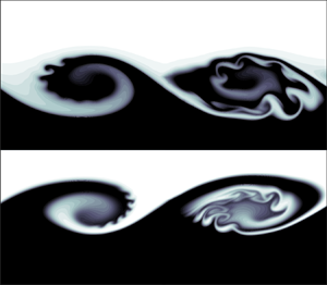This is illustrated in figure 2 which displays the azimuthal vorticity field of a KH vortex ring at the saturation time $T_s$ for the light, homogeneous and heavy jets. In agreement with figure 1, a significant depletion of base flow vorticity is observed on the outer side of the braid of the light jet, together with a slight increase of vorticity on the inner side. In the heavy jet, the local baroclinic production on the outer side of the braid yields a local maximum of vorticity of the same magnitude as that located in the vortex core. The deformation of the isocontours on the inner side of the heavy jet braid denotes a substantial local reduction of the azimuthal vorticity. This uneven redistribution of vorticity is intensified with increasing Atwood and Reynolds numbers as illustrated by the azimuthal vorticity of the same variable-density jets at $\textit {Re}=10\,000$ in figure 3. Increasing the Reynolds number results in sharper gradients of velocity and density which yield a layered distribution of the base flow vorticity as well as stronger baroclinic sources and sinks. Their effect on the base flow is visible at the saturation time where vorticity patches of opposite sign are observable on the inner side of the braid for the heavy jet and on the outer side for the light one.

Figure 1. Baroclinic torque distribution for a KH vortex ring at saturation time developing on (a) a light jet with $\textit {At}=-0.25$ and (b) a heavy one with $\textit {At}=0.25$. Points H and E denote the hyperbolic and elliptical stagnation points. The grey-shaded region corresponds to the domain where the base flow density is higher than $\rho _0$. Solid (dashed) contours correspond to positive (negative) values of the contoured quantity (here the baroclinic torque). Only the upper half-plane is shown and the jet axis corresponds to the lower bound. These conventions hold throughout the paper.

Figure 2. Azimuthal vorticity field of a KH vortex ring at the KH saturation time $T_s$ for (a) $\textit {At}=-0.25$, (b) $\textit {At}=0$ and (c) $\textit {At}=0.25$.

Figure 3. Temporal evolution of the azimuthal vorticity field of a perturbed round jet for $\textit {Re}=10\,000$ with $\textit {At}=-0.25$ (lower half-plane) and $\textit {At}=0.25$ (upper half-plane). When comparing in the entire meridian plane, the jet axis lies in the centre of the figure and this convention holds throughout the paper.

Another consequence, closely related to the base flow vorticity redistribution, lies in a significant change in the strain field. Figure 4 shows the local distribution of the Euclidean norm of the deviatoric strain rate tensor $\Vert {\boldsymbol{\mathsf{D}}}_0 \Vert _2$ for $t=0.8T_s,\,T_s,\,1.2T_s$ (see Appendix A for its definition). Before the KH saturation time, the maximum of the strain rate field is located in the braid region. For the light jet, it spreads also towards the vortex core and its magnitude is slightly lower than those observed for the homogeneous and heavy cases. At the saturation time, the light jet exhibits a strong intensification of its strain rate field in a region going from the vortex core to the outer side of the braid. A similar but less intense trend is observed in the homogeneous case. For the heavy jet ($\textit {At} = 0.25$), the strain rate field remains concentrated within the outer side of the braid, i.e. in the same region where the baroclinic torque is an active source term (see also figure 1b). After the KH saturation, i.e. $t=1.2T_s$, the magnitude of the strain rate in the light jet becomes significantly larger than those of the homogeneous and heavy cases and peaks in a narrow zone located in the outer part of the vortex ring between the elliptical and hyperbolic stagnation points.

Figure 4. Euclidean norm of the deviatoric strain rate tensor in the time interval $[0.8T_s,1.2T_s]$ for $\textit {At}=-0.25$, 0, 0.25 and $\textit {Re}=1000$. Dashed contours correspond to $20\,\%$ of the maximal absolute value of the base flow azimuthal vorticity $\varOmega _{\theta }$. The contour levels are the same for all figures.

2.3. Optimisation problem

The linear evolution of the three-dimensional perturbations $[\boldsymbol {u},\rho,p]$ that are likely to develop on the top of the variable-density KH vortex ring $[\boldsymbol {U},R,P]$ is now considered. We linearise the governing equations (2.1)–(2.3) around the two-dimensional base flow and we retain only the equations for the small-amplitude perturbations:

(2.8)\begin{gather} \frac{\partial {\rho}}{\partial t} ={-} ( \boldsymbol{U} \boldsymbol{\cdot} \boldsymbol{\nabla} {\rho} + {\boldsymbol{u}} \boldsymbol{\cdot} \boldsymbol{\nabla} R) - {\rho} (\boldsymbol{\nabla} \boldsymbol{\cdot} \boldsymbol{U} ) - R (\boldsymbol{\nabla} \boldsymbol{\cdot} \boldsymbol{u}), \end{gather}

(2.9)\begin{gather} \frac{\partial {\boldsymbol{u}}}{\partial t} ={-} (\boldsymbol{U} \boldsymbol{\cdot} \boldsymbol{\nabla} {\boldsymbol{u}} + {\boldsymbol{u}} \boldsymbol{\cdot} \boldsymbol{\nabla} \boldsymbol{U} ) - \frac{1}{R} \boldsymbol{\nabla} {p} + \frac{{\rho}}{R^2} \boldsymbol{\nabla} P + \frac{1}{\textit{Re} R} \boldsymbol{\Delta} {\boldsymbol{u}} \nonumber\\ \qquad - \frac{{\rho}}{\textit{Re} R^2} \boldsymbol{\Delta} {\boldsymbol{U}} + \frac{1}{3 \textit{Re} R} \boldsymbol{\nabla} (\boldsymbol{\nabla} \boldsymbol{\cdot} {\boldsymbol{u}}) - \frac{{\rho}}{3 \textit{Re} R^2} \boldsymbol{\nabla} (\boldsymbol{\nabla} \boldsymbol{\cdot} \boldsymbol{U}), \end{gather}

(2.10)\begin{gather} \boldsymbol{\nabla} \boldsymbol{\cdot} \boldsymbol{u} ={-} \frac{1}{\textit{Re} \textit{Sc}} \boldsymbol{\Delta} \left(\frac{\rho}{R}\right). \end{gather}

This linear system, referred to as the direct system, can be cast in the following compact form:

(2.11)\begin{equation} {\boldsymbol{\mathsf{N}}}_t \boldsymbol{\cdot} \boldsymbol{q} + {\boldsymbol{\mathsf{N}}}_c \boldsymbol{\cdot} \boldsymbol{q} + \frac{1}{\textit{Re}}{\boldsymbol{\mathsf{N}}}_d \boldsymbol{\cdot} \boldsymbol{q} = 0, \end{equation}

where $\boldsymbol {q}=[\boldsymbol {u},\rho,p]$ and the three matrix operators are the temporal operator ${\boldsymbol{\mathsf{N}}}_t$, the operator of coupling between the base flow and the perturbation ${\boldsymbol{\mathsf{N}}}_c$ and the diffusion operator ${\boldsymbol{\mathsf{N}}}_d$, respectively. Their expressions are detailed in Appendix B.

In the frame of non-modal stability analysis, the temporal behaviour of the perturbations is not prescribed and, considering the streamwise periodicity and the azimuthal homogeneity of the base flow, the disturbances are sought under the form

(2.12)\begin{equation} [u_r,u_{\theta},u_z,\rho,p](r,\theta,z,t)= \tfrac{1}{2} ([\tilde{u}_r,{\rm i} \tilde{u}_{\theta},\tilde{u}_z,\tilde{\rho},\tilde{p}](r,z,t) \,\mathrm{e}^{{\rm i}(\mu z+m\theta)} + {\rm c.c.} ), \end{equation}

where $m$ is the azimuthal wavenumber and $\mu \in [0, \, 1]$ the real Floquet exponent. We restrict here the search for perturbations that have the same streamwise periodicity as the base flow, i.e. $\mu = 0$. This is motivated by the experimental evidence that three-dimensional secondary instabilities involved in round jets develop in between two consecutive KH vortex rings. Furthermore, Klaassen & Peltier (Reference Klaassen and Peltier1991) and Fontane & Joly (Reference Fontane and Joly2008) found that the most unstable modes of both stratified and inhomogeneous mixing layers did not vary appreciably with non-zero Floquet exponent.

Amongst all possible perturbations likely to grow over the KH vortex ring, we look for those maximising the gain of kinetic energy $E$ over a prescribed period of time $[t_0,\,T]$:

(2.13)\begin{equation} G_E(T,t_0) = \frac{E(T)}{E(t_0)} = \frac{\Vert \boldsymbol{q}(T) \Vert_u}{\Vert \boldsymbol{q}(t_0) \Vert_u}, \end{equation}

where $t_0,\ T$ are called the injection and horizon times, respectively, and $\Vert \boldsymbol {\cdot } \Vert _u$ denotes the seminorm associated with the conventional inner product yielding the kinetic energy (see Appendix C). Following the work of Farrell (Reference Farrell1988), we look for the optimal perturbation with the maximal energy gain

(2.14)\begin{equation} \mathcal{G}_E(T,t_0) = \max_{\boldsymbol{q}(t_0)}\{G_E(T,t_0)\}, \end{equation}

over all the possible initial conditions $\boldsymbol {q}(t_0)$. Its determination resorts to solving an optimisation problem with constraints (Gunzburger Reference Gunzburger2002) enforcing the perturbation to be a solution of the linearised Navier–Stokes equations (2.11). The problem can be classically transformed into an optimisation problem without constraint using the variational method of the Lagrange multipliers (see Luchini & Bottaro Reference Luchini and Bottaro1998; Corbett & Bottaro Reference Corbett and Bottaro2000, Reference Corbett and Bottaro2001). This requires the derivation of the so-called adjoint equations (Schmid Reference Schmid2007) associated with the direct system (2.8)–(2.9):

(2.15)\begin{gather} -\frac{\partial {\rho}^{{{\dagger}}}}{\partial t} = \boldsymbol{U} \boldsymbol{\cdot} \boldsymbol{\nabla} {\rho}^{{{\dagger}}} + \frac{1}{R^2}{\boldsymbol{u}}^{{{\dagger}}} \boldsymbol{\cdot} \left[ \boldsymbol{\nabla} P - \frac{1}{\textit{Re}} \boldsymbol{\Delta} \boldsymbol{U} - \frac{1}{3\textit{Re}} \boldsymbol{\nabla} (\boldsymbol{\nabla} \boldsymbol{\cdot} \boldsymbol{U}) \right] - \frac{1}{\textit{Re} \textit{Sc} R} {\Delta} {p}^{{{\dagger}}}, \end{gather}

(2.16)\begin{gather} - \frac{\partial {\boldsymbol{u}^{{{\dagger}}}}}{\partial t} = [ \boldsymbol{U} \boldsymbol{\cdot} \boldsymbol{\nabla} {\boldsymbol{u}^{{{\dagger}}}} + {\boldsymbol{u}^{{{\dagger}}}} (\boldsymbol{\nabla} \boldsymbol{\cdot} \boldsymbol{U}) - \boldsymbol{u}^{{{\dagger}}} \boldsymbol{\cdot} \boldsymbol{\nabla} \boldsymbol{U} ^T ]+ \boldsymbol{\nabla} {p^{{{\dagger}}}} + R \boldsymbol{\nabla} \rho^{{{\dagger}}} \nonumber\\ + \frac{1}{\textit{Re}} \boldsymbol{\Delta} {\left( \frac{\boldsymbol{u}^{{{\dagger}}}}{R} \right)} + \frac{1}{3 \textit{Re}} { {\boldsymbol{\nabla}} \left[ \boldsymbol{\nabla} \boldsymbol{\cdot} \left( \frac{\boldsymbol{u}^{{{\dagger}}}}{R} \right) \right] }, \end{gather}

(2.17)\begin{gather} \boldsymbol{\nabla} \boldsymbol{\cdot} \left( {\frac{\boldsymbol{u}^{{{\dagger}}}}{R}} \right) = 0. \end{gather}

Likewise the direct system (2.11), the adjoint system can be reduced to the following compact form:

(2.18)\begin{equation} - {\boldsymbol{\mathsf{N}}}_t \boldsymbol{\cdot} \boldsymbol{q}^{{{\dagger}}} + {\boldsymbol{\mathsf{N}}}^{{{\dagger}}} _c \boldsymbol{\cdot} \boldsymbol{q}^{{{\dagger}}} + \frac{1}{\textit{Re}}{\boldsymbol{\mathsf{N}}}^{{{\dagger}}} _d \boldsymbol{\cdot} \boldsymbol{q}^{{{\dagger}}} = 0, \end{equation}

where $\boldsymbol {q}^{{\dagger} } = [\boldsymbol {u}^{{\dagger} },\rho ^{{\dagger} },p^{{\dagger} }]$. Solving the evolution of this dynamical system requires a backward-in-time integration as signified by the minus sign before the temporal operator ${\boldsymbol{\mathsf{N}}}_t$. The expressions for the adjoint matrix operator ${\boldsymbol{\mathsf{N}}}^{{\dagger} } _c$ of the coupling between the base flow and the disturbance and the adjoint diffusion operator ${\boldsymbol{\mathsf{N}}}^{{\dagger} } _d$ are given in Appendix B. An iterative procedure allows to determine the optimal perturbation and the corresponding optimal energy gain $\mathcal {G}_E$, as originally proposed by Luchini & Bottaro (Reference Luchini and Bottaro2001) and Corbett & Bottaro (Reference Corbett and Bottaro2001). An initial condition $\boldsymbol {q}(t_0)$ chosen as a white noise is integrated forward in time to the horizon time $T$ using the direct system (2.11). The initial white noise condition can be applied to every field of the perturbation, but we restrict it here to the velocity field because the objective is to maximise the kinetic energy gain from a purely kinematic initial perturbation. The resulting final state is used to compute the initial condition $\boldsymbol {q}^{{\dagger} }(T)$ for the adjoint system (2.18) which is integrated backward-in-time back to the injection time $t_0$. After an appropriate normalisation, this perturbation candidate at $t_0$ is used as the initial condition for the next direct-adjoint integration. Multiple iterations of this forward–backward loop converge eventually to the optimal perturbation. Both direct and adjoint systems are integrated with the linearised version of the two-dimensional three-components dealiased pseudo-spectral method used for the generation of the base flow. The outline of the optimisation algorithm is given in Appendix C and full details are provided in § 2.3.3 of Nastro (Reference Nastro2020). In practice, the convergence of this iterative optimisation algorithm is very quick and the solution is currently obtained in about 10 iterations.

2.4. Diagnostics

In order to understand the physical mechanisms associated with the energy growth of the optimal perturbations, we use diagnostics such as the evolution equation for the energy growth rate of the perturbation $\sigma _E = (1/E) \,\mathrm {d}E/\mathrm {d}t$. It is obtained straightforwardly from the transport equation for the perturbation kinetic energy $E = \Vert \boldsymbol {q} \Vert _u$ which reads

(2.19)\begin{align} \frac{\mathrm{d} E}{\mathrm{d} t} &={-}\underbrace{ \int_{\mathcal{V}} u_r u_z \left( \frac{\partial U_r}{\partial z} + \frac{\partial U_z}{\partial r}\right) \mathrm{d} \mathcal{V}}_{\varPi_{E_1}}- \underbrace{\int_{\mathcal{V}} \left( u^2_r \frac{\partial U_r}{\partial r} + u^2_{\theta} \frac{U_r}{r} + u^2_z \frac{\partial U_z}{\partial z} \right) \mathrm{d} \mathcal{V}}_{\varPi_{E_2}} \nonumber\\ &\quad +\underbrace{\int_{\mathcal{V}} \frac{\Vert \boldsymbol{u} \Vert}{2} (\boldsymbol{\nabla} \boldsymbol{\cdot} \boldsymbol{U}) \,\mathrm{d} \mathcal{V}}_{\varPi_{E_3}} - \underbrace{\int_{\mathcal{V}} \left( \frac{\boldsymbol{u}}{R} \boldsymbol{\cdot} \boldsymbol{\nabla} p \right) \mathrm{d} \mathcal{V}}_{\varPi_{E_4}} + \underbrace{\int_{\mathcal{V}} \frac{\rho}{R^2} \left( \frac{\boldsymbol{u}}{R} \boldsymbol{\cdot} \boldsymbol{\nabla} P \right) \mathrm{d} \mathcal{V}}_{\varPi_{E_5}} \nonumber\\ &\quad + \underbrace{\frac{1}{Re} \int_{\mathcal{V}} \phi_{\mu} \, \mathrm{d} \mathcal{V}}_{\varPi_{E_{\varPhi_1}}} + \underbrace{\frac{1}{Re} \int_{\mathcal{V}} \varPhi_{\mu} \, \mathrm{d} \mathcal{V}}_{\varPi_{E_{\varPhi_2}}}, \end{align}

where $\phi _{\mu }$ is the viscous dissipation coming from the perturbation velocity field defined by

(2.20)\begin{equation} \phi_{\mu} = \frac{1}{R} \left\{ \boldsymbol{u} \boldsymbol{\cdot} \boldsymbol{\Delta} \boldsymbol{u} + \frac{1}{3}[\boldsymbol{u} \boldsymbol{\cdot} \boldsymbol{\nabla} (\boldsymbol{\nabla} \boldsymbol{\cdot} \boldsymbol{u})] \right\}, \end{equation}

and $\varPhi _{\mu }$ is the viscous dissipation coming from the coupling with the base flow velocity field defined by

(2.21)\begin{equation} \varPhi_{\mu} ={-} \frac{\rho}{R^2} \left\{ \boldsymbol{u} \boldsymbol{\cdot} \boldsymbol{\Delta} \boldsymbol{U} + \frac{1}{3}[\boldsymbol{u} \boldsymbol{\cdot} \boldsymbol{\nabla} (\boldsymbol{\nabla} \boldsymbol{\cdot} \boldsymbol{U})] \right\}. \end{equation}

Different source/sink terms can be thus distinguished in (2.19): $\varPi _{E_1}$ is the energy production/destruction due to the base flow shear, $\varPi _{E_2}$ the energy production/destruction due to the base flow strain field, $\varPi _{E_3}$ the energy production/destruction due to the base flow dilatation, $\varPi _{E_4}$ the energy production/destruction due to the perturbation pressure gradient, $\varPi _{E_5}$ the energy production/destruction due to the base flow pressure gradient, $\varPi _{E_{\varPhi _1}}$ the viscous dissipation coming from the perturbation velocity field and $\varPi _{E_{\varPhi _2}}$ the viscous dissipation involving the base flow velocity field. The terms $\varPi _{E_3}$, $\varPi _{E_4}$, $\varPi _{E_5}$ and $\varPi _{E_{\varPhi _2}}$ are specific to the variable-density case, and both $\varPi _{E_4}$ and $\varPi _{E_5}$ terms correspond to the remnant of the baroclinic vorticity production in the kinetic energy equation.

It is also useful to derive the linearised version of the vorticity equation (2.4) which reads

(2.22)\begin{align} \frac{\partial {\boldsymbol{\omega}}}{\partial t} + \boldsymbol{U} \boldsymbol{\cdot} \boldsymbol{\nabla} \boldsymbol{\omega} + \boldsymbol{u} \boldsymbol{\cdot} \boldsymbol{\nabla} \boldsymbol{\varOmega} &= \boldsymbol{\varOmega} \boldsymbol{\cdot} \boldsymbol{\nabla} {\boldsymbol{u}} + {\boldsymbol{\omega}} \boldsymbol{\cdot} \boldsymbol{\nabla} \boldsymbol{U} -\boldsymbol{\varOmega} (\boldsymbol{\nabla} \boldsymbol{\cdot} \boldsymbol{u}) - \boldsymbol{\omega} (\boldsymbol{\nabla} \boldsymbol{\cdot} \boldsymbol{U}) \nonumber\\ &\quad + \boldsymbol{b} + \frac{1}{Re R} \left( \boldsymbol{\Delta} \boldsymbol{\omega} - \frac{\rho}{R} \boldsymbol{\Delta} \boldsymbol{\varOmega} - \boldsymbol{\phi}_R - \boldsymbol{\phi}_{\rho} \right), \end{align}

where $\boldsymbol {b}$ is the linearised baroclinic torque defined by

(2.23)\begin{equation} \boldsymbol{b} = \frac1R \boldsymbol{\nabla} R \times \underbrace{\left( \frac1R \boldsymbol{\nabla} p - \frac{\rho}{R^2} \boldsymbol{\nabla} P \right)}_{(i)} + \boldsymbol{\nabla} \left( \frac{\rho}{R} \right) \times \underbrace{\frac1R \boldsymbol{\nabla} P}_{(ii)}, \end{equation}

$\boldsymbol {\phi }_R$ and $\boldsymbol {\phi }_{\rho }$ are the coupling between the base flow density field and the perturbation diffusion and the coupling between the perturbation density field and the base flow diffusion, respectively. They are defined as follows:

(2.24)\begin{gather} \boldsymbol{\phi}_R = \frac1R \boldsymbol{\nabla} R \times \left( \boldsymbol{f}_D - \frac{\rho}{R} \boldsymbol{\mathcal{F}}_D \right), \end{gather}

(2.25)\begin{gather}\boldsymbol{\phi}_{\rho} = \boldsymbol{\nabla} \left( \frac{\rho}{R} \right) \times \boldsymbol{\mathcal{F}}_D, \end{gather}

where $\boldsymbol {\mathcal {F}}_D = \boldsymbol {\Delta } \boldsymbol {U} + \frac {1}{3} \boldsymbol {\nabla } (\boldsymbol {\nabla } \boldsymbol {\cdot } \boldsymbol {U} )$ and $\boldsymbol {f}_D = \boldsymbol {\Delta } \boldsymbol {u} + \frac {1}{3} \boldsymbol {\nabla } (\boldsymbol {\nabla } \boldsymbol {\cdot } \boldsymbol {u} )$.

As already done for the baroclinic torque (2.5) in the base flow vorticity equation, the pressure terms (i) and (ii) in (2.23) can be replaced by the flow accelerations in the limit of $\textit {Re} \rightarrow \infty$

(2.26)\begin{equation} \boldsymbol{b} = \boldsymbol{a} \times \frac1R \boldsymbol{\nabla} R + \boldsymbol{A} \times \boldsymbol{\nabla} \left( \frac{\rho}{R} \right) \end{equation}

with $\boldsymbol {a}$ and $\boldsymbol {A}$ the perturbation and base flow accelerations:

(2.27a)\begin{gather} \boldsymbol{a} = \frac{\partial {\boldsymbol{u}}}{\partial t} + \boldsymbol{U} \boldsymbol{\cdot} \boldsymbol{\nabla} {\boldsymbol{u}} + {\boldsymbol{u}} \boldsymbol{\cdot} \boldsymbol{\nabla} \boldsymbol{U} ={-} \frac{1}{R} \boldsymbol{\nabla} {p} + \frac{{\rho}}{R^2} \boldsymbol{\nabla} P, \end{gather}

(2.27b)\begin{gather}\boldsymbol{A} = \frac{\partial {\boldsymbol{U}}}{\partial t} + \boldsymbol{U} \boldsymbol{\cdot} \boldsymbol{\nabla} {\boldsymbol{U}} ={-} \frac{1}{R} \boldsymbol{\nabla} {P}. \end{gather}

The equation for the perturbation enstrophy $Z= \int _{\mathcal {V}} \boldsymbol {\omega }^* \boldsymbol {\cdot } \boldsymbol {\omega } \,\mathrm {d} \mathcal {V}$ is derived from the vorticity transport equation (2.22) to evaluate its growth rate $\sigma _Z = (1/Z) \,\mathrm {d}Z/\mathrm {d}t$ budget:

(2.28)\begin{align} \frac{\mathrm{d} Z}{\mathrm{d} t} &= \underbrace{\int_{\mathcal{V}} {\omega_r} {\omega_z} \left( \frac{\partial U_r}{\partial z} + \frac{\partial U_z}{\partial r}\right) \mathrm{d} \mathcal{V}}_{\varPi_{Z_1}} + \underbrace{\int_{\mathcal{V}} \left( \omega^2_r \frac{\partial U_r}{\partial r} + \omega^2_{\theta} \frac{U_r}{r} + \omega^2_z \frac{\partial U_z}{\partial z} \right) \mathrm{d} \mathcal{V}}_{\varPi_{Z_2}} \nonumber\\ &\quad - \underbrace{\int_{\mathcal{V}} \frac{\Vert \boldsymbol{\omega} \Vert^2}{2} (\boldsymbol{\nabla} \boldsymbol{\cdot} \boldsymbol{U})\, \mathrm{d} \mathcal{V}}_{\varPi_{Z_3}} - \underbrace{\int_{\mathcal{V}} [ \boldsymbol{\omega} \boldsymbol{\cdot} (\boldsymbol{u} \boldsymbol{\cdot} \boldsymbol{\nabla \varOmega})^T ]\, \mathrm{d} \mathcal{V}}_{\varPi_{Z_4}} + \underbrace{\int_{\mathcal{V}} [ \boldsymbol{\omega} \boldsymbol{\cdot} (\boldsymbol{\varOmega} \boldsymbol{\cdot} \boldsymbol{\nabla u})^T ]\, \mathrm{d} \mathcal{V}}_{\varPi_{Z_5}} \nonumber\\ &\quad - \underbrace{\int_{\mathcal{V}} (\boldsymbol{\omega} \boldsymbol{\cdot} \boldsymbol{\varOmega}) ( \boldsymbol{\nabla} \boldsymbol{\cdot} \boldsymbol{u}) \,\mathrm{d} \mathcal{V}}_{\varPi_{Z_6}} + \underbrace{\int_{\mathcal{V}} (\boldsymbol{\omega} \boldsymbol{\cdot} \boldsymbol{b}) \,\mathrm{d} \mathcal{V}}_{\varPi_{Z_7}} + \underbrace{\frac{1}{Re} \int_{\mathcal{V}} \phi_Z \,\mathrm{d} \mathcal{V}}_{\varPi_{Z_{\varPhi_1}}} + \underbrace{\frac{1}{Re} \int_{\mathcal{V}} \varPhi_Z \,\mathrm{d} \mathcal{V}}_{\varPi_{Z_{\varPhi_2}}}, \end{align}

where

(2.29a,b)\begin{equation} \phi_Z = \frac{1}{R} [ \boldsymbol{\omega} \boldsymbol{\cdot} ( \boldsymbol{\Delta} \boldsymbol{\omega} - \boldsymbol{\phi}_{\rho} )] \quad \text{and} \quad \varPhi_Z ={-} \frac{\rho}{R^2} \left[ \boldsymbol{\omega} \boldsymbol{\cdot} \left( \boldsymbol{\Delta} \boldsymbol{\varOmega} + \frac{R}{\rho} \boldsymbol{\phi}_R \right) \right]. \end{equation}

In particular, we can distinguish different source/sink terms in (2.28): $\varPi _{Z_1}$ is the enstrophy production/destruction due to the base flow shear, $\varPi _{Z_2}$ the enstrophy production/destruction due to the base flow strain, $\varPi _{Z_3}$ the enstrophy production/destruction due to the base flow dilatation, $\varPi _{Z_4}$ the enstrophy production/destruction due to the perturbation stretching, $\varPi _{Z_5}$ the enstrophy production/destruction due to the base flow vorticity advection, $\varPi _{Z_6}$ the enstrophy production/destruction due to the perturbation dilatation, $\varPi _{Z_7}$ is the baroclinic enstrophy production/destruction, $\varPi _{Z_{\varPhi _1}}$ the viscous dissipation coming from the perturbation vorticity field and $\varPi _{Z_{\varPhi _2}}$ the viscous dissipation resulting from the base flow vorticity field.

3.1. The universal first phase

We first consider the early evolution of optimal perturbations growing from the initial time of the base flow evolution, i.e. $t_0=0$, on both an unperturbed parallel jet experiencing viscous spreading and a jet perturbed by a low-amplitude KH mode. The Reynolds number is $\textit {Re} = 1000$ and the Atwood number is $\textit {At}=-0.25$ and $\textit {At}=0.25$ for the light and heavy jets, respectively. Figure 5 displays the temporal evolution of the energy gain $\mathcal {G}_E$ of perturbations optimised for $T=T_s/2$ and $T=T_s$, for azimuthal wavenumbers ranging from $m=0$ to $m=5$. The time variable is normalised by the KH saturation time $T_s$. For comparison, the energy gains corresponding to the homogeneous case have been added (Jimenez-Gonzalez et al. Reference Jimenez-Gonzalez, Brancher and Martinez-Bazan2015; Nastro et al. Reference Nastro, Fontane and Joly2020). When perturbations are optimised for half the KH saturation time, the energy curves are all superimposed reaching a value of $\mathcal {G}_E \approx 10^2$, whether disturbances grow over an unperturbed or a perturbed jet. In the interval $[0,T_s/2]$, the Atwood number does not have much influence on the perturbation growth either, because the energy gain follows the same route for all cases. For $t>T_s/2$, the optimal growth becomes more sensitive to the Atwood number as the energy evolution corresponding to the light and heavy jets slightly deviate from the one of the homogeneous case. The difference between the perturbed and unperturbed jet base flows becomes also perceptible after half the KH saturation time. For this reason, we consider $T_s/2$ as a milestone that separates the evolution of optimal disturbances in two periods: an initial time interval $[0,T_s/2]$ characterised by a universal growth of the perturbation energy regardless of the density variations and the low-amplitude KH wave, and a second period starting at $t\approx T_s/2$ when the evolution of the optimal perturbation starts becoming sensitive to the Atwood number and the nonlinear development of the KH mode. This initial energy growth has been recognised to be universal in all shear flows by Farrell & Ioannou (Reference Farrell and Ioannou1993) and has also been observed in the case of variable-density mixing layers (Lopez-Zazueta et al. Reference Lopez-Zazueta, Fontane and Joly2016). It is associated with energy growth driven by a combination of Orr and lift-up mechanisms, as discussed in the following.

Figure 5. Temporal evolution of the energy gain $\mathcal {G}_E$ for optimal perturbations growing over a diffusing Michalke profile (thick lines) and over a perturbed jet (thin lines) for $\textit {At}=-0.25$ (red), $\textit {At}=0$ (black) and $\textit {At}=0.25$ (blue) and six azimuthal wavenumbers $m\in [0;5]$. The thick continuous lines in the figure corresponding to $m=0$ represent the temporal evolution of the energy gain of the primary KH modes. The symbols are located at the horizon time of each energy curve.

We now focus on the spatial distribution of the kinetic energy of perturbations optimised for $T = T_s/2$. Figure 6(a) shows the temporal evolution of the kinetic energy field $E$ from the injection time $t_0=0$ to $T=T_s/2$ for the optimal perturbation growing over a parallel jet under viscous spreading (lower half-plane) and a jet perturbed by the KH mode (upper half-plane), both in the light jet case at $\textit {At}=-0.25$. We consider the same values of azimuthal wavenumber $m$ as in figure 5. Figure 6(b) displays similarly the kinetic energy of optimal perturbations in the case of a heavy jet characterised by $\textit {At}=0.25$. At injection time, the optimal perturbations take the form of two elongated layers oriented along the direction of maximal compression of the base flow very similar to those observed in the homogeneous case (see Nastro et al. Reference Nastro, Fontane and Joly2020). In the diffusing parallel jet, these structures are symmetric whereas the addition of a primary KH instability in the base flow induces an asymmetry between the two layers: that located in the region that will form the outer side of the braid is more energetic. The difference in the energy peak between the two layers is more pronounced for the heavy jet than for the light one. For later times at $At=-0.25$, the larger peak relocates from the outer side towards the inner side of the braid which hosts the main source of baroclinic vorticity production. This loss of symmetry reflects the one observed in the base flow. Despite that asymmetry, the optimal perturbations are not very sensitive to the presence of the KH wave in the time interval $[0,T_s/2]$ because the energy gains are all overlapping and the spatial distribution of the kinetic energy is quite comparable for both the unperturbed and the perturbed jet, as evidenced in figure 6. The base flow mean shear leads to a gradual deformation of these layers before their complete reorientation along the direction of maximal stretching of the base flow. This is a result of the combined action of the Orr (Reference Orr1907) and lift-up (Ellingsen & Palm Reference Ellingsen and Palm1975) mechanisms which are responsible for the transient energy growth of these so-called ‘OL’ perturbations, as already observed in homogeneous jets (Nastro et al. Reference Nastro, Fontane and Joly2020) and in plane shear layers (Arratia et al. Reference Arratia, Caulfield and Chomaz2013; Lopez-Zazueta et al. Reference Lopez-Zazueta, Fontane and Joly2016). The intensification/attenuation of one or the other layer over time conforms to the evolution of the base flow mean shear, itself driven by the uneven baroclinic vorticity sources and sinks, as described in section § 2.2. As a consequence, the optimal perturbation evolution differs between the light and the heavy jet. At $t=T_s/2$, the most energetic layer is located in the inner side of the braid in the light jet whereas it is located in the outer side for the heavy jet (see also the close-up views in figure 7 for the optimal perturbation with $m=3$). Nevertheless, this uneven distribution of energy between the two layers is balanced because the energy gain remains comparable to that obtained in the homogeneous case. Interestingly, this asymmetry is emphasised with increasing azimuthal wavenumber $m$ in the heavy jet and decreased in the light one.

Figure 6. Early time evolution of the kinetic energy field $E$ of optimal perturbations growing over a diffusing unperturbed parallel jet (lower half-plane) and a perturbed jet (upper half-plane), at (a) $\textit {At}=-0.25$ and (b) $\textit {At}=0.25$, for all the azimuthal wavenumbers considered in figure 5. The horizon time for the optimisation is $T=T_s/2$. The energy is normalised by the maximum value at each time and 10 equally spaced contour levels are used.

Figure 7. Close-up views taken from figure 6 for $m=3$ and $T=T_s/2$.

The initial growth of these ‘OL’ perturbations ruled by the combination of the two shear-driven transient mechanisms is generic of shear flows. The amplification of the radial velocity $u_r$ by the Orr mechanism can strengthen the streamwise rolls involved in the production of longitudinal velocity streaks at play in the lift-up mechanism (Farrell & Ioannou Reference Farrell and Ioannou1993). Simultaneously, the intensification of the axial velocity $u_z$, fed by the lift-up mechanism, enhances the azimuthal vorticity and, as a consequence, affects the circulation whose conservation substantiates the Orr mechanism according to the Kelvin theorem.

3.2. Second period $[T_s/2,2T_s]$

We now consider the temporal evolution of the optimal perturbations in the period $[T_s/2,2T_s]$ during which the axisymmetric shear layer progressively rolls up into a nonlinear KH vortex ring. Figure 8 shows the optimal energy gain $\mathcal {G}_E$ as a function of the normalised horizon time $T/T_s$, for azimuthal wavenumbers $m$ up to five.

Figure 8. Optimal energy gain $\mathcal {G}_E$ as a function of the time ratio $T/T_s$ for $\textit {At}=-0.25$ (red), $\textit {At}=0$ (black) and $\textit {At}=0.25$ (blue), and for the same six azimuthal wavenumbers considered in figure 5. The thick continuous lines in the figure for the axisymmetric perturbation ($m=0$), correspond to the temporal evolution of the energy gain of the specific primary KH modes.

The optimal energy gains of disturbances growing over a homogeneous vortex ring, as obtained by Nastro et al. (Reference Nastro, Fontane and Joly2020), have been added for comparison. For $\textit {At}=-0.25$ the helical mode is the global optimal similar to the homogeneous case ($\textit {At}=0$). For the heavy jet ($\textit {At}=0.25$), the helical perturbation is the global optimal up to $T \approx 1.8T_s$, after which the $m=2$ and $m=3$ modes present larger energy gains. The paths of energy growth of both the axisymmetric and helical perturbations do not show significant sensitivity to the Atwood number. The energy gain of the axisymmetric mode decreases after the KH saturation time, whereas the energy of the helical mode continues to grow slowly after $T_s$. The picture is quite different for modes with larger azimuthal wavenumbers. For $m \geq 2$, the disturbances growing over a heavy jet experience a substantial increase of their energy gains after the KH saturation time (especially for $m=3$) on a similar trend as the post-saturation growth observed in the homogeneous case. As their amplification before saturation is more efficient than for their homogeneous counterparts there is an offset between these two cases after $T_s$. However, in the light jet case, the energy gains of the perturbations are saturating if not decreasing for $T>T_s$. As a result, the optimal perturbations for $\textit {At}=-0.25$ present smaller energy gains for $T>1.5T_s$ than those of the perturbations growing on the homogeneous jet.

We now focus on the spatial distribution of the kinetic energy $E$ of the optimal perturbations during the time interval $[T_s,2T_s]$ as displayed in figure 9. The upper and lower half-planes correspond to the heavy and light jet configurations, respectively. The axisymmetric optimal perturbation for both $\textit {At} = -0.25$ and $\textit {At} = 0.25$ entails a linear transient growth relying on the 2D Orr mechanism, not exploited by the primary mode. This Orr-driven disturbance saturates due to the absence of any three-dimensional relay mechanism for a secondary energy growth. At this quite low Reynolds number, the optimal growth of the helical mode $m=1$ is found to be particularly unaffected by the modifications of the base flow field by density effects nor by the contribution of the linearised baroclinic torque. For larger azimuthal wavenumbers, the optimal perturbations in the heavy jet experience the combined development of E-type and H-type instabilities starting with a predominance of the elliptical mode at $m=1$ and evolving towards a preponderance of the hyperbolic one at $m=5$. This change in regions of energy growth with increasing $m$ is similar to what has been observed in the homogeneous case (Nastro et al. Reference Nastro, Fontane and Joly2020). In the light jet, if the helical perturbation stands as an E-type instability, the structure of the perturbations at larger azimuthal wavenumbers differs from that observed in the homogeneous and heavy cases. Shortly after the KH saturation time $T_s$, we note a progressive concentration of the energy growth in a region located between the vortex core and the braid (see figure 9 for $m \geq 2$ at $t=5T_s/4$) which corresponds precisely to the base flow region hosting the largest strain intensity, as evidenced in § 2.2 (see figure 4).

Figure 9. Temporal evolution of the kinetic energy field $E$ of optimal perturbations from $t=3T_s/4$ to $t=2T_s$ for various azimuthal wavenumbers with $\textit {At}=0.25$ (upper half-plane) and $\textit {At}=-0.25$ (lower half-plane). The optimisation time is $T=3T_s/2$. The energy is normalised by the maximum value at each time for a given Atwood number and 10 equally spaced contour levels are used.

The structure of the optimal perturbation with $m=4$ for $\textit {At}=-0.25$ is illustrated in figure 10. In particular, we consider the spatial distribution of the three velocity components of the optimal perturbation at $t=1.2T_s$, i.e. the time for which the light jet exhibits the relative maximum of the strain rate field. The axial velocity $u_z$ is shown in the meridian plane whereas the radial $u_r$ and azimuthal $u_{\theta }$ velocity components are represented in the crosswise plane corresponding to the maximal value of the perturbation kinetic energy identified in figure 9 and tagged as section K–K in figure 10. The axial velocity is mainly concentrated in this region between the vortex core and the outer side of the braid where the base flow strain field is maximum (see figure 4). In the corresponding crosswise plane, periodic radial ejections/injections are observed and the azimuthal velocity is in quadrature with the radial velocity. This spatial distribution of perturbation velocity components in the K–K plane thus complies with the standard pattern of strained longitudinal vortices. Figure 10(d,e) displays the axial vorticity $\omega _z$ in two distinct crosswise planes: a first lying in the braid in line with the hyperbolic stagnation point (section H–H) and the second in the vortex core in line with the elliptical stagnation point (section E–E). In both cross-sections, four pairs of counter-rotating streamwise vortices concentrated along the mean outer isopycnal line are visible. They span the entire longitudinal extent of the jet and they induce the radial velocity field observed in the plane K–K. This mechanism of energy growth conforms to the mechanism of side-jet generation based on vortex induction advocated by Monkewitz & Pfizenmaier (Reference Monkewitz and Pfizenmaier1991) and, later, by Brancher et al. (Reference Brancher, Chomaz and Huerre1994). Our results thus plead in favour of the standard scenario, at least for a moderate negative Atwood number. In addition, the key ingredient of the distinct mechanism proposed by Lopez-Zazueta et al. (Reference Lopez-Zazueta, Fontane and Joly2016), i.e. the convergence/divergence towards the braid saddle point of longitudinal velocity streaks of opposite sign, is not retrieved as seen from figure 10(c), at least for this value of the Reynolds number.

Figure 10. (a) Radial, (b) azimuthal and (c) axial velocity components and (d,e) axial vorticity of the optimal perturbation characterised by $m=4$ at $t=T=1.2T_s$ and $At=-0.25$. Points K, E and H indicate the location of the peak value of the perturbation energy, the elliptical and hyperbolic stagnation points, respectively. The radial and azimuthal velocity components are displayed in the crosswise plane K–K, whereas the axial velocity in the meridian plane. The axial vorticity $\omega _z$ is represented in two crosswise planes: (d) plane H–H and (e) plane E–E. Contour levels are normalised by the local maximal absolute value, solid (respectively, dashed) contours correspond to positive (respectively, negative) values.

3.3. Influence of the Reynolds number

In this section, we discuss the effect of the Reynolds number $\textit {Re}$ on the optimal perturbations. Figure 11 displays the temporal evolution of the energy gain $\mathcal {G}_E$ for disturbances optimised for $T=3T_s/2$ at $\textit {Re}=10\,000$ compared with those obtained at $\textit {Re}=1000$, for the same azimuthal wavenumbers. Owing to the corresponding diminution of the viscous dissipation, the increase in Reynolds number results in higher energy gains but the extra growth is larger for variable-density situations compared with the homogeneous one, except for $m=1$ where the homogeneous perturbation shows an energy gain larger than that corresponding to the heavy jet case. For $m \geq 2$, this extra energy growth benefits more to the optimal perturbations of the light jet and yields a different hierarchy between the perturbations. At $\textit {Re}=10\,000$ the optimal energy gain for $\textit {At}=-0.25$ is comparable to that for $\textit {At}=0.25$ whereas it is lower at $\textit {Re}=1000$. The largest energy gain is attributed to the double-helix disturbance for the light jet and to the $m=3$ mode for the heavy jet, at least for $t$ up to $T=1.5T_s$. However, the strong similarity between the amplification curves for $m \geq 2$ at a given $At$ is symptomatic of a loss of scale selectivity of the underlying base flow. As evidenced experimentally by Liepmann & Gharib (Reference Liepmann and Gharib1992) and retrieved by the stability analysis of Nastro et al. (Reference Nastro, Fontane and Joly2020) in the homogeneous case, increasing the Reynolds number hampers selection of the azimuthal periodicity of secondary instabilities.

Figure 11. Temporal evolution of the energy gain $\mathcal {G}_E$ of optimal perturbations at $\textit {Re}=10\,000$ (solid lines) and $\textit {Re}=1000$ (dashed lines) growing over a perturbed jet with $\textit {At}=-0.25$ (red), $\textit {At}=0$ (black), $\textit {At}=0.25$ (blue) and for six azimuthal wavenumbers $m\in [0;5]$. The thick lines in the figure for $m=0$ represent the temporal evolution of the energy gain of the corresponding primary KH modes. The symbols are located at the horizon time of each energy curve.

Figure 12 presents the time evolution of the kinetic energy field $E$ from the injection time to $T=3T_s/2$ for the optimal $m=4$ perturbation developing on the heavy jet (upper half-plane) and on the light jet (lower half-plane). The optimal disturbance exhibits the same structure than that observed at $\textit {Re}=1000$ but the two layers are much thinner as expected. The evolution during the first phase in the time interval $[t_0,T_s/2]$ reflects the shear-driven growth due to the Orr and lift-up mechanisms. However, as soon as $t=T_s/2$, when the disturbance is aligned with the maximal stretching direction of the base flow, the localisation of the energy maximum starts to move towards the side of the braid which benefits from the baroclinic vorticity production (see figure 3). The subsequent evolution shows a strong correlation of the localisation of the kinetic energy of the perturbation with the regions of the base flow where the baroclinic vorticity production is active, at least up to saturation time. At the horizon time $T=3T_s/2$, the production and base flow advection of the energy results in an optimal response essentially located at the outer periphery of the vortex core for the light jet case and at the inner periphery of the billow for the heavy jet.

Figure 12. Temporal evolution of the kinetic energy field $E$ of the optimal perturbation with $m=4$ and $T=3T_s/2$ growing over the heavy one (upper half-plane) and the light jet (lower half-plane). Same conventions as in figure 9.

For the light jet case, looking at the contribution of each velocity component to the evolution of the perturbation energy gain in figure 13(a), it can be seen that the energy growth is mainly due to the increase of the axial velocity $u_z$. Figure 13(b) shows also that the growth of the perturbation enstrophy is clearly driven by the azimuthal vorticity $\omega _{\theta }$ which is almost two orders of magnitude larger than the other vorticity components at the horizon time. The corresponding budgets for the energy and enstrophy growth rates rate are given in figure 13(c,d) according to (2.19) and (2.22). Although the initial growth of both quantities is driven by the base flow shear conversion owing to the Orr and lift-up mechanisms, the growth in the second phase for $t\approx 7 T_s/10$ results from a combination of the base flow strain conversion, measured by $\sigma _{E_{2}}$ for the energy and $\sigma _{Z_{4+5}}$ for the enstrophy, and the action of the baroclinic torque, i.e. the terms $\sigma _{E_{4+5}}$ for the energy and $\sigma _{Z_7}$ for the enstrophy. As stated by (2.26), the azimuthal component $b_{\theta }$ of the linearised baroclinic torque results from the sum of two contributions:

(3.1)\begin{equation} b_{\theta} = \underbrace{a_z \frac1R \frac{\partial R}{\partial r} - a_r \frac1R \frac{\partial R}{\partial z}}_{b_{\theta_1}} + \underbrace{A_z \frac{\partial}{\partial r} \left( \frac{\rho}{R} \right) - A_r \frac{\partial}{\partial z} \left( \frac{\rho}{R} \right)}_{b_{\theta_2}} . \end{equation}

As observed also in the plane mixing layer by Lopez-Zazueta et al. (Reference Lopez-Zazueta, Fontane and Joly2016, figure 13), although the first term $b_{\theta _1}$ is predominant in the early development of perturbations, the second phase proceeds with baroclinic production from the term $b_{\theta _2}$ (not shown) associated with large-amplitude density perturbation. Its evolution from $t=3T_s/4$ to $t=3T_s/2$ is illustrated on the first row of figure 14 for the $m=4$ optimal perturbation. At $t=3 T_s/4$, it consists of two thin layers of density perturbation of opposite sign located along the braid. Combined with the local base flow acceleration, it yields the specific structure of azimuthal baroclinic torque supported by the sketch of vectors at $t=3 T_s/4$ shown in the second row of figure 14. This spatial distribution of $b_{\theta }$ in the form of two layers of opposite sign along the braid on either side of the saddle point yields a similar azimuthal vorticity distribution. The structuration of the perturbation azimuthal vorticity driven by the component $b_{\theta _2}$ of the linearised baroclinic torque continues up to the horizon time as indicated by the strong similarity between the two fields. According to Biot–Savart induction, these vorticity layers yield elongated patches of longitudinal velocity at their interface as seen in the last row of figure 14. At $T=3T_s/2$, the disturbance axial velocity field consists of two parallel elongated layers of opposite sign located at the outer periphery of the vortex ring where the perturbation kinetic energy is concentrated, see figure 12. This mechanism of secondary energy growth is the same as that identified by Lopez-Zazueta et al. (Reference Lopez-Zazueta, Fontane and Joly2016) in the variable-density mixing layer but the structuration of the optimal perturbation at the horizon is here quite different.

Figure 13. Temporal evolution of (a) the kinetic energy growth rate $\sigma _E$ and (b) the enstrophy growth rate $\sigma _Z$ for the optimal perturbation at $m=4$ and $At=-0.25$ with their corresponding budgets (c) and (d), according to (2.19) and (2.28), respectively. The horizon time is $T=3T_s/2$ (as indicated by the symbol on each curve).

Figure 14. Temporal evolution of density $\rho$, azimuthal component of the baroclinic torque $b_{\theta }$, azimuthal vorticity $\omega _{\theta }$ and axial velocity $u_z$ of the optimal $m=4$ perturbation during the time interval $[3T_s/4,3T_s/2]$. The perturbation is optimised for $T=3T_s/2$ with $At=-0.25$.

As for the heavy jet case, figure 15 shows similarly the energy (a) and enstrophy (b) gains up to $t=2T_s$ along with the relative contribution of each velocity/vorticity component for the same parameters, $m=4$ and $T=1.5T_s$. The corresponding contributions to the temporal evolution of the energy and enstrophy growth rates according to (2.19) and (2.22) are shown in figures 15(c) and 15(d). We denote a strong anisotropy in the energy and enstrophy growths which are born by the axial velocity and the azimuthal vorticity, respectively. Beyond the first phase of universal shear-driven growth ending around $t \approx 7T_s/10$, the energy increase is due to the baroclinic torque $\sigma _{E_{4+5}}$ combined alternatively with the base flow strain term $\sigma _{E_2}$ and the base flow shear conversion term $\sigma _{E_1}$. As in the light jet case, post-saturation enstrophy growth relies on baroclinic vorticity production $\sigma _{Z_7}$ and the base flow strain conversion $\sigma _{Z_{4+5}}$. As illustrated in figure 16, the associated physical mechanism is the same as for the optimal perturbation in the light jet. The structure of the perturbation azimuthal vorticity is driven by the component $b_{\theta _2}$ of the linearised baroclinic torque which results from the combination of the local two-dimensional base flow acceleration field and the perturbation density, as illustrated by the sketch of vectors at $t=T_s$ in the second row of figure 14. The distribution of $\omega _{\theta }$ leads to two elongated axial velocity layers which are localised at the horizon time at inner periphery of the KH vortex core, where the perturbation kinetic energy is concentrated in figure 12.

Figure 15. Temporal evolution of (a) the kinetic energy growth rate $\sigma _E$ and (b) the enstrophy growth rate $\sigma _Z$ for the optimal perturbation with $m=4$ and $At=0.25$ with their corresponding budgets (c) and (d), according to (2.19) and (2.28), respectively. The horizon time is $T=3T_s/2$ (as specified by the symbol on each curve).

Figure 16. Temporal evolution of density $\rho$, azimuthal component of the baroclinic torque $b_{\theta }$, azimuthal vorticity $\omega _{\theta }$ and axial velocity $u_z$ of the optimal $m=4$ perturbation at $At=0.25$ during the time interval $[3T_s/4,3T_s/2]$. The horizon time is $T=3T_s/2$.

This optimal perturbation leading to an intense shear layer on the braid outer side for the light jet and on the inner one for the heavy jet contrasts with that observed at smaller Reynolds number. Therefore, this instability could be involved in the side-jet generation and the difference in the location of the perturbation between the light and heavy jets could be related to the observation of side jets in the light case only.

For both the light and heavy jet, the increase in Reynolds number yields higher energy gains which are associated with the same physical mechanism first identified by Lopez-Zazueta et al. (Reference Lopez-Zazueta, Fontane and Joly2016) in the variable-density mixing layer. Here, the optimal response takes the form of two layers of axial velocity both localised on the inner side of the KH vortex core in the case of the heavy jet and on the outer side for the light jet configuration. The density variation thus turns the paradigm of saddle-centred counter-rotating streamwise vortices into a quite different optimal response. However, it is slightly different from the longitudinal velocity streaks of opposite sign along the braid on either side of the hyperbolic saddle point observed in the plane variable-density mixing layer. Its stands as a third candidate path to three-dimensionalisation for variable-density shear flows but its connection with side-jet generation remains unclear.

3.4. Influence of the injection time and fractal KH breakups

In § 3.1 we found that the Atwood number $\textit {At}$ has no influence on the early evolution of optimal perturbations. We now delay the instant of perturbation beyond the first universal phase to elucidate secondary growth mechanisms over a well developed but unperturbed KH roll-up. An injection time of $t_0=7 T_s/10$ is thus selected in order to leave out the short-time energy growth driven by both the Orr and lift-up mechanisms. Figure 17 displays the time evolution of the energy gain $\mathcal {G}_E$ for the corresponding optimal perturbations for all the azimuthal wavenumbers considered here. The horizon time is $T=2T_s$ and two Reynolds numbers are considered, i.e. $\textit {Re}=1000$ and $\textit {Re}=10\,000$. For $\textit {Re}=1000$, the energy gain reached at the horizon time is, as expected, much lower than when growth benefits from the powerful transient growth resulting from shear-driven OL mechanisms in the initial stage (before $7T_s/10$). This observation holds whatever the Atwood number in the present range, presumably because mass diffusion at unitary Schmidt number and vorticity diffusion in the base flow both prevent the secondary growth that is strikingly steep for a higher Reynolds number. Although homogeneous optimal perturbations for $\textit {Re}=10\,000$ only weakly benefit from higher shear and lower dissipation, the variable-density optimal growth with postponed injection exhibits intense monotonic energy growth, with energy gains as high as around $10^6$ at horizon time. We have verified (not shown) that the delayed energy growth of secondary perturbations at $\textit {Re}=1000$ resorts to standard E-type and H-type secondary instabilities. For the base flow rolling-up into a high-Reynolds-number variable-density vortex ring, the supplementary growth of energy is very likely to be associated with a different physical mechanism. Figure 18 shows the contributions to the temporal evolution of the energy and enstrophy growth rates according to (2.19) and (2.28) for the axisymmetric optimal perturbations ($m=0$) optimised for $T = 2T_s$. The initial growth is seen to be driven by the base flow shear conversion identified by term $\sigma _{E_1}$ but it is shortly replaced by the term $\sigma _{E_{4+5}}$ in (2.19) and $\sigma _{Z_7}$ in (2.28) which correspond to the baroclinic vorticity production. In agreement with the energy gains plotted in figure 17, the energy and enstrophy growth rates of the disturbances developing on the light jet are slightly higher than those of the perturbations for the heavy jet. Figure 19 presents the temporal evolution of the fields of density and azimuthal vorticity of the axisymmetric optimal perturbation for both the light and the heavy jet. The optimal excitation consists of small elongated spanwise vorticity and density patches of alternate sign located along the outer side of the braid for the heavy jet and the inner side of the braid for the light jet. It corresponds to the region where the base flow baroclinic torque represents a source of azimuthal vorticity $\varOmega _{\theta }$ (see figure 1). This structure is characteristic of the secondary KH instability first observed by Reinaud et al. (Reference Reinaud, Joly and Chassaing2000). The subsequent time evolution shows that the disturbance is convected towards the core of the KH vortex ring. The same spatial distribution is observed for all non-zero azimuthal wavenumbers. As demonstrated by Reinaud et al. (Reference Reinaud, Joly and Chassaing2000), the baroclinic secondary KH instability is triggered when inertial baroclinic vorticity production supersedes the stabilising effect of stretching along the vorticity braid. Because baroclinic vorticity production benefits from the increase in Reynolds number for fixed Atwood and Schmidt numbers, the secondary KH instability is expected to emerge at some flow-dependant Reynolds number. We deduce that the onset of secondary baroclinic KH instability occurs between $\textit {Re}=1000$ and $\textit {Re}=10\,000$ in the present case. Lopez-Zazueta et al. (Reference Lopez-Zazueta, Fontane and Joly2016) retrieved the secondary KH mode in the variable-density mixing layer for a Reynolds number $\textit {Re}=1000$, based on the shear layer width. This is consistent with the present value of $\textit {Re}=10\,000$ based on the jet radius, provided that the aspect ratio of the present jet is $\alpha =10$. It is demonstrated in Lopez-Zazueta et al. (Reference Lopez-Zazueta, Fontane and Joly2016) that the secondary KH instability developing over a planar mixing-layer is a two-dimensional mechanism for which oblique versions with non-zero spanwise wavenumbers exhibit weaker energy growth than the two-dimensional one, i.e. that with a streamwise wave vector perpendicular to base-flow KH roll-ups. We stress that in the present situation, the growth that builds up on the same mechanism, is only slightly weaker for non-zero azimuthal wavenumbers. As seen from figure 17, the response to optimal perturbations with oblique wave vectors is following almost exactly the same route in terms of energy growth over a large range of azimuthal wavenumbers suggesting a loss of azimuthal selectivity. The proposed temporal approach with delayed injection gives an estimate of the potential of energy growth and of the associated receptivity to ambient perturbations downstream the nozzle of a spatially developing jet. However, because real-world perturbations are not controlled two-dimensional ones, we conjecture that baroclinic secondary KH instabilities are more likely to occur in real jets than in plane mixing layers.

Figure 17. Temporal evolution of the energy gain $\mathcal {G}_E$ of optimal perturbations injected at $t_0=7T_s/10$ for $\textit {Re}=10\,000$ (solid lines) and $\textit {Re}=1000$ (dashed lines) growing over a perturbed jet at $\textit {At}=-0.25$ (red), $\textit {At}=0$ (black) and $\textit {At}=0.25$ (blue) and for the same six azimuthal wavenumbers considered in figure 16. The thick lines in the figure for $m=0$ represent the temporal evolution of the energy gain of the corresponding primary KH modes. The symbols are located at the horizon time of each energy curve.

Figure 18. Temporal evolution of (a,b) the kinetic energy growth rate $\sigma _E$ and (c,d) the enstrophy growth rate $\sigma _Z$ with their different contributions according to (2.19) and (2.28) for the axisymmetric optimal perturbation growing over a KH vortex ring with (a,c) $\textit {At}=-0.25$ and (b,d) $\textit {At}=0.25$. As evidenced by the symbol on each curve, the horizon time is $T=2T_s$.

Figure 19. Linear evolution of the axisymmetric optimal perturbation ($m=0$) for $\textit {Re}=10\,000$ with $\textit {At}=0.25$ (upper half-plane) and $\textit {At}=-0.25$ (lower half-plane) from $t=t_0=7T_s/10$ to $t=T=2T_s$ in terms of (upper row) density $\rho$ and (lower row) azimuthal vorticity $\omega _{\theta }$. The quantities are normalised by the corresponding maximum value at each time for a given Atwood number.

We choose to illustrate this path for secondary growth even beyond the linear stage by means of a nonlinear simulation stemming from a base flow perturbed with the axisymmetric optimal perturbation. This results into the development of a secondary KH instability as shown in figure 20 for both the light and the heavy KH vortex ring. In the light jet, the inner side of the braid experiences undulations yielding the development of secondary KH breakups within the primary vortex ring. In the heavy jet, a similar evolution happens on the outer side of the braid (see figures 20a and 20b). At later times we also observe the emergence of a curvature-driven Rayleigh–Taylor instability, similar to the one observed by Joly et al. (Reference Joly, Fontane and Chassaing2005). As illustrated by figures 20(e) and 20(f), it occurs at the interface between the jet and the surrounding fluid due to centripetal acceleration induced by the curvature of fluid particle trajectories. It is evidenced by the formation of opposite-sign secondary vortices (as opposed to like-signed ones for the secondary KH instability, see figures 20c and 20d) yielding mushroom-shaped density contours, as evidenced by figures 20(g) and 20(h). The late stages of evolution show a fast increase of the length of isopycnic lines due to the stretching between secondary vortices, both promoting mixing between the two fluids.

Figure 20. Temporal development of the secondary KH instabilities for $\textit {Re}=10\,000$ with $\textit {At}=0.25$ (upper half-plane) and $\textit {At}=-0.25$ (lower half-plane) for $t=4T_s/5,\,T_s,\,6T_s/5,\,7T_s/5$: (a,b) close-up insets on the KH vortex ring at $t=T_s$ and (c,d) relative to $t=7T_s/5$, as evidenced by the square-shaped regions showing where the zoom is located. All pictures display the flow density field $R$.

Though thriving in the nonlinear regime, the oblique secondary KH instability cannot be related to side ejections in any way. Primary or secondary KH billows are organised as rows of corotating vortices along shear layers, yielding a strong deformation of the hyperbolic regions. As secondary structures developing in the present context over a primary KH vortex ring, they promote local mixing but they cannot induce radial velocities. In contrast, the onset of oblique secondary KH instability is likely to be the reason of the disappearance of side jets at large Reynolds numbers and of the particularly short route to turbulence observed in the light jets experiments of Fontane (Reference Fontane2005).