


1. Introduction
The roll-up of trailing vortices associated with aircraft wing tips is of significance to safety considerations when regulating the landing frequency of aircraft (Spalart Reference Spalart1998), where strong persisting vortices can roll lighter aircraft faster than can be resisted by the use of ailerons (Vernon Reference Vernon1999). This practical interest has motivated much of the relevant literature concerning vortex pairs (see Leweke, Le Dizès & Williamson (Reference Leweke, Le Dizès and Williamson2016) for a review), with further scientific interest due to the elementary configuration of the vortices in the flow problem. Specifically, the roll-up results in a pair of counter-rotating parallel vortices in its wake, which exhibits complex two- and three-dimensional behaviours. The study of the interactions and instabilities of these vortex pairs can be used to understand the often more complicated vortical flows observed in nature, such as in the case of sunspot formation (Matthews, Hughes & Proctor Reference Matthews, Hughes and Proctor1995) and in the engineering industry, such as in the instance of active control of flows in axial compressors (Bae, Breuer & Tan Reference Bae, Breuer and Tan2005).
Furthermore, the addition of a ground plane below the vortex pair, as in the case of wing-tip vortices generated on take-off and landing, modifies the vortex pair trajectory and interaction (Lamb Reference Lamb1932), and involves complex viscous dynamics at the boundary (Doligalski Reference Doligalski1994) which can be comparable to that of oblique ring-wall impingement (Asselin & Williamson Reference Asselin and Williamson2017). The resultant physics is of interest across all scales of fluid dynamics, from micro-scale coherent turbulent structures at walls (Hussain Reference Hussain1986) to vortex generators (Anderson & Gibb Reference Anderson and Gibb2008), through to large aircraft wakes interacting with runways (see Gerz, Holzäpfel & Darracq (Reference Gerz, Holzäpfel and Darracq2002) for a review).
The two-dimensional dynamics of inviscid counter-rotating point-vortex pairs in the presence of walls was first studied by Lamb (Reference Lamb1932), who noted that outside of wall effect, equal strength counter-rotating pairs descend by mutual induction at a constant speed of  $U_0=\varGamma /2{\rm \pi} b$ as a function of their circulation
  $\varGamma$ and vortex spacing
  $b$. Upon interaction with the wall, the vortices move apart along a hyperbolic trajectory. In the case of finite-core viscous vortex pairs, however, the vortices were observed to deviate from the hyperbolic trajectory by ‘rebounding’ from the wall, first explained by Harvey & Perry (Reference Harvey and Perry1971). As the descending vortex pair interacts with the wall, a boundary layer with opposite-signed vorticity forms. Once the adverse pressure gradient in the boundary layer is strong enough, the secondary vorticity rolls up into discrete vortex structures, and the primary vortices ‘rebound’ and rise (Kramer, Clercx & van Heijst Reference Kramer, Clercx and van Heijst2007). The secondary vortices then spiral around the primary vortices and further sets of ‘rebounds’ have been observed (Orlandi Reference Orlandi1990).
Unlike two-dimensional vortex pairs however, the dynamics of three-dimensional vortex pairs is substantially altered by the introduction of cooperative three-dimensional instabilities. The counter-rotating vortex pairs undergo two widely studied instabilities distinguished by their respective wavelengths.
The long-wavelength instability is characterised by symmetric sinusoidal displacement of the vortex tubes with peak growth rates depending on the relative core size  $a/b$ for wavelengths between 6 and 10 times the vortex spacing
  $b$. This displacement can be observed in high-altitude aircraft wakes, where the wing-tip vortices are visualised by condensation (Scorer & Davenport Reference Scorer and Davenport1970). The instability was first studied outside of wall effect by Crow (Reference Crow1970), who described the instability through the displacements of vortex filaments by Biot–Savart induction. The analysis of Crow (Reference Crow1970) illustrated that the instability consists of three mechanisms: first, the self-induced rotation of the deformations of the vortices which were observed by Kelvin (Reference Kelvin1880); second, the strain field induced by the vortex pair that consists of maximum stretching in the
  $45^{\circ }$ direction, where the angle is measured from an imaginary line that joins the two vortices; and third, a resonance mechanism between the perturbations of both vortices that induces stretching and rotation opposite to that of the self-induced rotation. For a specific set of relative core size
  $a/b$, angle of the plane on which the instability lies
  $\theta$ and displacement wavelength
  $\lambda /b$, the rotation effects cancel and the amplitude of the instability grows. The amplitude of the wavy instability continues to grow on the plane until the troughs of the sinusoids of both vortices connect periodically. This reconnection subsequently results in the formation of elliptic vortex rings, observed experimentally by Leweke & Williamson (Reference Leweke and Williamson2011). The long-wavelength instability has been studied extensively in the context of aircraft wakes with, for example, the inclusion of turbulence and stratification (Misaka et al. Reference Misaka, Holzäpfel, Hennemann, Gerz, Manhart and Schwertfirm2012). Crow's analysis has been extended by Bliss (Reference Bliss1970) and Widnall, Bliss & Zalay (Reference Widnall, Bliss, Zalay, John, Arnold and Milton1971) to consider finite-core vorticity distributions based on a Batchelor vortex and has been applied to a large number of flow configurations including vortex arrays (Robinson & Saffman Reference Robinson and Saffman1982) and collisions of vortex rings (Lim & Nickels Reference Lim and Nickels1992). Crouch (Reference Crouch1997) and Fabre & Jacquin (Reference Fabre and Jacquin2000) investigated the stability of two trailing vortex pairs as would be located behind an aircraft wing in the flaps-down configuration, finding the Crow instability to be significantly accelerated with the potential to be initiated by perturbing the inner pair.
The short-wavelength instability is characterised by the growth of perturbations that modify the structure of the vortex core itself, with wavelength of similar order to the vortex core size. The vortex filament approach employed by Crow (Reference Crow1970) is insufficient due to this scaling, and the existence of the short-wavelength instability was first illustrated by Moore & Saffman (Reference Moore and Saffman1975), who established the excitement of short-wavelength Kelvin modes through an externally imposed strain field on a general axisymmetric vortex distribution. Tsai & Widnall (Reference Tsai and Widnall1976) further confirmed this in the context of a Rankine vortex and found that the growth of these modes stems from the strain field induced by each vortex resulting in elliptic rather than circular streamlines. Subsequent investigations found that this ‘elliptic’ instability applies to Lamb–Oseen vortex profiles (Fabre, Sipp & Jacquin Reference Fabre, Sipp and Jacquin2006) and Batchelor vortices with axial flow (Lacaze, Ryan & Le Dizès Reference Lacaze, Ryan and Le Dizès2007). Kerswell (Reference Kerswell2002) summarises the analytical framework describing the elliptic instability. The short-wave perturbations were further shown to influence the dynamics of vortex pairs generated by aircraft wings through the breaking of the symmetry of the long-wavelength mode, and through an increase of the growth rate of the Crow instability by approximately  $20\,\%$ (Leweke & Williamson Reference Leweke and Williamson1998). Direct numerical simulations of the elliptic instability in counter-rotating pairs was performed by Laporte & Corjon (Reference Laporte and Corjon2000) that recovered the features of the work of Leweke & Williamson (Reference Leweke and Williamson1998). Le Dizès & Laporte (Reference Le Dizès and Laporte2002) extended the theoretical results to Gaussian vortex pairs and obtained expressions for the growth rate of the short-wave instability as a function of global flow parameters.
Upon wall interaction, the secondary vortices also become unstable (see Luton & Ragab Reference Luton and Ragab1997; Harris & Williamson Reference Harris and Williamson2012) and Asselin & Williamson (Reference Asselin and Williamson2017) demonstrated that the three-dimensional instabilities strongly influence the evolution of the viscous vortex pair/wall interaction problem.
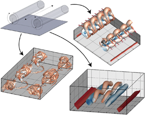
Specifically, the long-wavelength instability was found to modify the three-dimensional wall-bounded dynamics depending on the extent of the instability upon wall interaction. At relatively small initial heights, the growth of the instability was found to be inhibited by the presence of the ground. As the Crow instability develops, regions of the vortex tubes closest to the wall interact with the boundary layer first, with a corresponding increase in local pressure driving flow axially away from these regions. Asselin & Williamson (Reference Asselin and Williamson2017) identified three modes of interaction as a function of the initial height the vortices were generated above the wall, all of which resulted in the formation of structures comparable to those observed in vortex-ring impingement, studied experimentally by Lim (Reference Lim1989) and numerically by Cheng, Lou & Luo (Reference Cheng, Lou and Luo2010). These modes of interaction were triggered by small perturbations in the vortices, with the amplitude of these perturbations upon wall interaction determining the subsequent physics. The resultant dynamics, in particular the formation of vortex ‘tongues’ and ‘rings’, are almost completely unrecognisable when compared to the unbounded Crow instability, implying that the optimal perturbation mechanism of the wall-bounded interaction for various perturbation amplitudes is of significant interest.
The consideration of Batchelor vortices as asymptotic solutions to the linearised Navier–Stokes equations for trailing-line vortices downstream of an aircraft (Batchelor Reference Batchelor1964) is an important extension to the stability analysis of vortex pairs as better approximations to experimental aircraft wakes. The addition of axial flow in the case of the Batchelor vortex allows for positive instability growth with respect to both inviscid (Ash & Khorrami Reference Ash and Khorrami1995) and viscous (Fabre & Jacquin Reference Fabre and Jacquin2004) perturbations on an isolated vortex without the induced strain field of the second vortex. The addition of the second vortex further complicates the stability picture, with a modified elliptic instability that changes depending on the degree of axial flow (Lacaze et al. Reference Lacaze, Ryan and Le Dizès2007). Lacaze et al. (Reference Lacaze, Ryan and Le Dizès2007) demonstrated that axial flow damps the most resonant Kelvin modes and introduces new combinations of resonant Kelvin modes that become more unstable with increasing axial flow. For strong axial flow, the growth rate of the swirling jet instability (Delbende & Rossi Reference Delbende and Rossi2005) dominates and the nonlinear evolution of the Batchelor vortex pair changes, where the instability is dominated by inviscid negative helical modes.
In the context of aircraft landing safety, accelerating the growth of the wake instabilities can alleviate hazards posed by the trailing vortices. The ‘optimal perturbation’, or the perturbation that generates the largest perturbation energy growth over a period of time, gives insight into the conditions necessary to best accelerate the instability (Barkley, Blackburn & Sherwin Reference Barkley, Blackburn and Sherwin2008). Optimal growth analysis has been applied to a variety of flow configurations (see, for example, Blackburn, Barkley & Sherwin Reference Blackburn, Barkley and Sherwin2008; Abdessemed et al. Reference Abdessemed, Sharma, Sherwin and Theofills2009). This direct adjoint technique has been further applied by Pradeep & Hussain (Reference Pradeep and Hussain2006) to consider an arbitrary initial perturbation in the case of singular Lamb–Oseen vortices, who found that the optimal perturbations take the form of vortical spirals at the outer region of the vortex, which excite bending waves within the core, with the physical mechanism explained by Antkowiak & Brancher (Reference Antkowiak and Brancher2007) for a single vortex. In the case of vortex pairs, initial studies exciting the vortex pair at wavelengths characteristic of the cooperative instabilities found that the instability process could be greatly accelerated (Crow & Bate Reference Crow and Bate1976). Brion, Sipp & Jacquin (Reference Brion, Sipp and Jacquin2007) extended on these studies through an optimal perturbation investigation and found that the characteristic time of the Crow instability could be reduced by a factor of roughly two through optimal linear perturbation of the base flow. Brion et al. (Reference Brion, Sipp and Jacquin2007) realised the importance of the two stagnation (or hyperbolic) points in the amplification of the Crow instability, where the leading stagnation point was found to form vortex rings that optimally induce the long-wave bending mode. Donnadieu et al. (Reference Donnadieu, Ortiz, Chomaz and Billant2009) continued the study of transient growth over a range of wavenumbers and investigated the behaviour at smaller times and for the anti-symmetric case, where the trailing stagnation point was found to be important. Johnson, Brion & Jacquin (Reference Johnson, Brion and Jacquin2016) analysed the nonlinear response of a counter-rotating vortex pair to the optimal linear perturbation determined by Brion et al. (Reference Brion, Sipp and Jacquin2007), finding a periodically evolving vortex-ring state. An accelerated instability was observed at large initial perturbation amplitudes resulting in rapid decay of coherency. Further studies have considered optimal growth of co-rotating vortex pairs (Mao, Sherwin & Blackburn Reference Mao, Sherwin and Blackburn2012) and four-vortex configurations (Fabre, Jacquin & Loof Reference Fabre, Jacquin and Loof2002). A variety of passive and active physical controls have been proposed for the breakdown of tip vortices (Greenblatt Reference Greenblatt2012) and four-vortex systems (Crouch Reference Crouch2005), taking optimal amplification into account.
Recently, linear optimal perturbations have been applied to the case of vortex/wall interaction. Stuart, Mao & Gan (Reference Stuart, Mao and Gan2016) investigated the transient growth associated with wall generated secondary vorticity through the study of a single Batchelor vortex near the ground. Wakim et al. (Reference Wakim, Jacquin, Brion and Dolfi-Bouteyre2017) examined a pair of counter-rotating Lamb–Oseen vortices interacting with a ground plane through optimal perturbation studies involving two-dimensional perturbations for a small number of time horizons. Wakim et al. (Reference Wakim, Jacquin, Brion and Dolfi-Bouteyre2017) proposed two control strategies for optimal forcing of the vortex pair; one with significant gains in perturbation kinetic energies and the other employing an active blowing/suction method at the ground to maximise the lateral position of the vortices.
A complete picture of the optimal perturbation and control of vortex pairs interacting with the ground is yet to be attained. As the influence of three-dimensional instabilities on the dynamics of the vortex pair/wall interaction has been shown to drastically alter the resultant dynamics (Asselin & Williamson Reference Asselin and Williamson2017), understanding the influence of three-dimensional perturbations is critical to the flow problem.
This research seeks to fill the gaps in our understanding by considering the optimal perturbation and transient growth of a counter-rotating vortex pair interacting with a wall to three-dimensional perturbations. The article is organised as follows: first the problem definition and numerical approach is described in § 2; then the base flow study is discussed in § 3; the results of the linear transient energy growth follows in § 4, with direct numerical simulation employed to study the nonlinear evolution of the vortex pair with finite magnitude optimal perturbations in § 5. The article ends with conclusions in § 6.
2. Problem formulation
This study considers the optimal growth of an equal strength counter-rotating pair of Lamb–Oseen vortices located above a ground plane, motivated by a trailing vortex pair formed from wing-tip vortices interacting with a runway.
The flow problem is governed by the incompressible Navier–Stokes equations
 \begin{gather} \boldsymbol{\nabla} \boldsymbol{\cdot} \boldsymbol{u} = 0, \end{gather}
 \begin{gather} \frac{\partial \boldsymbol{u}}{\partial \tau} + \left(\boldsymbol{u} \boldsymbol{\cdot} \boldsymbol{\nabla} \right) \boldsymbol{u} = -\boldsymbol{\nabla} p + \frac{2{\rm \pi}}{Re} \nabla^2 \boldsymbol{u}, \end{gather}
where  $\boldsymbol {u}$ is the velocity field scaled by the initial descent velocity
  $U_0=\varGamma _0/(2{\rm \pi} b_0)$,
  $\tau$ is the time non-dimensionalised by the time taken for the vortex pair to descend a unit separation distance
  $\tau =t\varGamma _0/(2{\rm \pi} b_0^2)$ and
  $p$ is the kinematic pressure scaled by
  $U_0^2$. The Reynolds number is defined by the circulation and the length scale is based on the vortex spacing
  $b$:
$b$:
 \begin{equation} Re=\frac{\varGamma}{\nu}. \end{equation}
 The vortices are modelled by the superposition of two Lamb–Oseen vortices separated by distance  $b$, alongside two image vortices to ensure no flow through the ground plane. Each vortex is fully defined by
 \begin{equation} \varOmega_z=\frac{\varGamma}{{\rm \pi} a_0^2}\exp{\left(-\frac{r^2}{a_0^2}\right)}, \end{equation}
where  $\varOmega _z$ is the axial vorticity field,
  $\varGamma$ is the circulation,
  $r$ is the radial distance from the vortex core and
  $a_0$ is the initial characteristic core radius. The characteristic core radius increases in time due to diffusion and for a single vortex may be determined by
  $a=\sqrt {a_0^2+4\nu t}$, where
  $\nu$ is the fluid's kinematic viscosity.
The initial Reynolds number is set to  $Re=3125$, large enough to demonstrate the formation of vortex tongues observed by Asselin & Williamson (Reference Asselin and Williamson2017) (see § 5). In line with the study of Leweke & Williamson (Reference Leweke and Williamson2011), the initial core size is set to
  $a_0/b_0=0.23$.
Although each individual vortex satisfies the governing equations, the superposition of the two initial velocity fields does not. To account for this, the vortices are generated six separation distances ( $h/b_0=6.0$) above the wall, and the transient analysis is initiated from the point at which the vortices are located five separation distances above the wall, which gives ample time for the vortices to satisfy the Navier–Stokes equations (see Sipp, Jacquin & Cosssu Reference Sipp, Jacquin and Cosssu2000). In particular, this relaxation period allows the individual vortex cores to relax to a semi-periodic state and for initial oscillations to die out (also see Le Dizès & Verga Reference Le Dizès and Verga2002; Roy et al. Reference Roy, Schaeffer, Le Dizès and Thompson2008). The initial vortex height is taken to be consistent with the first mode of interaction observed by Asselin & Williamson (Reference Asselin and Williamson2017) and as a reasonable estimate to critical aircraft wake vortex formation. It is noted that the height at which the vortices are generated is non-critical, as it is the amplitude of the instability upon wall interaction which dictates the dynamics (Asselin & Williamson Reference Asselin and Williamson2017). Thus, given that the instability has ample time to develop, increasing the amplitude of the instability is effectively analogous to increasing the height at which the vortices form. The time taken for the vortices to descend this distance is found to be
  $t=6.50$, slightly longer than the
  $t=2{\rm \pi}$ predicted by theory due to cross-diffusion engendered circulation loss. At
  $h/b_0=5.0$, the core radii of the vortices are found to be
  $a=0.255$ by computing the vorticity polar moment,
 \begin{equation} a^2=\frac{\int_{x>0}((x-b/2)^2+(y-(h/b_0))^2)\varOmega_z\, \textrm{d}V}{\int_{x>0}\varOmega_z\, \textrm{d}V}, \end{equation}
and the instantaneous velocity of  $U=0.143$ is found by locating the vortices at
  $t=6.50 \pm 0.01$ to compute the streamlines in the moving reference frame alongside the instantaneous circulation
  $\varGamma =2{\rm \pi} b U=0.916$, where the vortex spacing
  $b$ has increased slightly to
  $b=1.02$. The instantaneous Reynolds number at
  $h/b_0=5.0$ can therefore be approximated as
  $Re=3125({\varGamma }/{\varGamma _0}) \approx 2860$. However, integrating the vorticity over the right half of the domain gives a value of
  $\varGamma = 0.945$ at the release position.
The boundary conditions are taken to be representative of the physical problem. The lower-wall boundary condition is of a no-slip type, and the lateral and upper boundaries are located far enough from the vortex pair such that as the vortex system is integrated forward in time, the velocity field at the boundary remains close to that of the initial vortex dipole.
2.1. Base flow
The flow is numerically solved on a semi-plane  $(x,y\geq y_{{wall}})$ normal to the axial direction
  $(z)$. The base flow is taken to be two dimensional and evolves with time to interact with the ground plane (figure 1). The direct numerical simulation (DNS) technique employs a spectral-element method to spatially discretize the domain, with high-order Lagrangian tensor-product polynomial basis functions used allowing for spatial refinement to be selected based on the order of the tensor-product interpolating polynomials. The equations are integrated in time using a fractional-step method accounting separately for the advection, pressure and diffusion terms of the Navier–Stokes equations (see Thompson, Hourigan & Sheridan Reference Thompson, Hourigan and Sheridan1996; Thompson et al. Reference Thompson, Hourigan, Cheung and Leweke2006). This technique, described in more detail by Karniadakis & Triantafyllou (Reference Karniadakis and Triantafyllou1992), allows for the advantages of spectral convergence whilst maintaining the flexibility of
  $h$-type convergence (Karniadakis & Sherwin Reference Karniadakis and Sherwin2005). For the three-dimensional simulations, the variation of variables in the spanwise direction is through a Fourier decomposition; again see Thompson et al. (Reference Thompson, Hourigan and Sheridan1996) and the references therein.

Figure 1. The two-dimensional unperturbed base flow of a viscous equal strength counter-rotating vortex pair spaced apart by distance  $b$ and with core radius
  $a/b_0=0.23$ interacting with a wall. The vortex pair is initially located at
  $(x,y)=({\pm }0.5b_0, 6.0b_0)$ and descends by mutual induction to the ground plane located at
  $y=0$. The transient growth study is initiated
  $(T=0)$ at the point at which the vortex pair has descended to
  $h/b_0=5.0$, and the resultant wall interaction is illustrated at times of
  $(a)$
$(a)$ $T=20$,
  $(b)$
$(b)$ $T=30$,
  $(c)$
$(c)$ $T=40$,
  $(d)$
$(d)$ $T=50$,
  $(e)$
$(e)$ $T=60$,
  $(f)$
$(f)$ $T=70$,
  $(g)$
$(g)$ $T=80$ and
  $(h)$
$(h)$ $T=90$. Positive vorticity is shown in red, negative in blue.
For finite perturbation amplitude studies (see § 5), the initial optimal perturbation field from the linear transient growth study is superimposed onto the base flow prior to forward time integration. Various amplitudes are considered, defined by the ratio of initial perturbation to base flow energy  $A=\sqrt {E_p/E_b}$ in the domain, where the kinetic energy of the perturbation and base fields integrated over the domain are given by the inner products
  $E_b(\boldsymbol {u})=(\boldsymbol {u},\boldsymbol {u})/2=\left (\int _\varOmega \boldsymbol {u}\boldsymbol {\cdot }\boldsymbol {u}\,\textrm {d}V\right )/2$ and
  $E_p(\boldsymbol {u'})=\left (\boldsymbol {u'},\boldsymbol {u'}\right )/2=\left (\int _\varOmega \boldsymbol {u'}\boldsymbol {\cdot }\boldsymbol {u'}\,\textrm {d}V\right )/2$, respectively. These quantities can be accurately calculated using the same quadrature techniques required for the application of the spectral-element method.
Furthermore, for finite perturbation amplitude studies, the trajectory of the primary vortex is obtained by locating the maximum vorticity of the primary vortex. The circulation is likewise calculated by taking the line integral of the velocity field along contours representing 5 % of the maximum vorticity of the primary vortices. In both cases, the Q-criterion is used to identify the primary vortex, such that secondary vorticity is excluded from the analysis.
2.2. Linear perturbations
The general solution to the flow field can be decomposed into the sum of a base flow and perturbation component such that  $\boldsymbol {u}=\boldsymbol {\bar {U}}+\boldsymbol {u}'$,
  $p=\bar {P}+p'$. Substituting these expressions into the Navier–Stokes equations (2.1) and (2.2) and omitting nonlinear products of the perturbation components results in the linearised Navier–Stokes equations. The result of this procedure differs only from the original governing equations by the nonlinear advection term which becomes
  $-\left (\boldsymbol {u'} \boldsymbol {\cdot } \boldsymbol {\nabla }\right )\boldsymbol {\bar {U}}-\left (\boldsymbol {\bar {U}}\boldsymbol {\cdot }\boldsymbol {\nabla }\right )\boldsymbol {u'}$, and can therefore be efficiently integrated forward in time with similar techniques to the nonlinear equations.
Furthermore, the forthcoming transient growth analysis necessitates integration of the adjoint linearised equations backwards in time:
 \begin{gather} \boldsymbol{\nabla} \boldsymbol{\cdot} \boldsymbol{u}^* = 0, \end{gather}
 \begin{gather} -\frac{\partial \boldsymbol{u^*}}{\partial \tau} - \boldsymbol{U} \boldsymbol{\cdot} \boldsymbol{\nabla} \boldsymbol{u}^* + \boldsymbol{u}^* \boldsymbol{\cdot} \left( \boldsymbol{\nabla} \boldsymbol{U}\right)^T = - \boldsymbol{\nabla} p^* + \frac{2{\rm \pi}}{Re} \nabla^2 \boldsymbol{u}^*. \end{gather}
Here the superscript  $*$ denotes the adjoint perturbation field of the corresponding variable.
The assumption of spatial periodicity in the axial direction allows for a further simplification of the disturbance fields, which can be decomposed through a Fourier series expansion in the axial direction  $z$ such that
 \begin{equation} \left[\boldsymbol{u'},p,\boldsymbol{u'}^*,p^*\right]=\int_{-\infty}^{\infty} \left[\boldsymbol{\hat{u}},\hat{p},\hat{\boldsymbol{u}}^*,\hat{p}^*\right]\textrm{e}^{\textrm{i}kz}\,\textrm{d}k, \end{equation}
which allows for the decoupling of Fourier modes with different axial wavenumbers  $k=2{\rm \pi} /\lambda$, where
  $\lambda$ is the wavelength of the mode respectively. Both the perturbation vorticity and spatial eigenmodes are derived from the two-dimensional Fourier modes
  $\hat {\boldsymbol {u}}$.
2.3. Transient growth formulation
Optimal transient growth is based on the maximum growth of perturbation energy in the flow up to a finite-time horizon  $T$. The forward time integration of a given perturbation field over a specific time interval
  $0\leq t \leq T$ can be reformulated as the eigenvalue problem
  $\boldsymbol {\boldsymbol {u'}(T)}=\mathscr {A}\boldsymbol {u'(0)}$, where the
  $\mathscr {A}$ operator represents the state transition between the initial and time horizon perturbation fields. Likewise, the adjoint operator
  $\mathscr {A}^*$ evolves the adjoint perturbation field governed by (2.6) and (2.7) backwards in time from the time horizon
  $t=T$ to
  $t=0$.
In addition to calculated optimal growth modes, modal solutions were also obtained to compare their associated amplification rates to optimal transient growth. These modal solutions were obtained for the base flow at  $h/b_0=5.0$ after adding a vertical velocity equal to the descent velocity of the vortex pair and freezing the base flow to stop diffusion. A linear stability analysis was run for various
  $kb$ to find the two peaks, and the maximally amplified long- (Crow) and short-wavelength (elliptic) modal perturbation fields were subsequently evolved alongside the original base flow to determine the energy growth for these two cases. Note that the maximally amplified long- and short-wavelength modal solutions were found to have growth rates and preferred wavelengths of
  $kb = 0.91$ and
  $9.0$ and
  $\sigma \tau = 0.77$ and
  $1.03$, respectively. These values are slightly different from but close to the corresponding theoretical values given in figure 2, presumably with the difference due to the strong interaction of the initially closely spaced vortex pair.

Figure 2. Theoretical modal growth rates of unbounded equal strength, counter-rotating vortex pairs for the parameters considered in this article. The long-wavelength Crow mode (- - -) has a peak growth rate of  $\sigma \tau =0.81$ for
  $kb=0.81$. The elliptic curves illustrate the inviscid predictions (—), and the viscous predictions of Le Dizès & Laporte (Reference Le Dizès and Laporte2002) (-.-.) and Leweke et al. (Reference Leweke, Le Dizès and Williamson2016) (
 $\cdots$) for the parameters detailed in § 2, i.e.
  $\nu =1/3125$,
  $\varGamma ={\pm }0.916$,
  $a=0.255$ and
  $b=1.02$. The peak growth rates of the first branch of the elliptic instability are
  $\sigma \tau =1.42, 1.03,0.73$ at
  $kb=8.91,8.58,8.31$ for the inviscid and two viscous predictions, respectively. The inserted images show the calculated axial vorticity distributions of the long- and short-wavelength modes.
The technique employed in this study to compute the optimal transient growth is described by Barkley et al. (Reference Barkley, Blackburn and Sherwin2008), and involves sequential forward and backwards time integration of the linearised and linearised adjoint Navier–Stokes fields to the horizon time and back until convergence of the optimal initial conditions. The optimal perturbation problem is one which maximises the energy growth for a specific time horizon  $T$ such that
  $G(T)=\max ({E_p(T)}/{E_p(0)})$, where the initial perturbation field is normalised to unity. It can be shown that
  $G(T)$ can be obtained through the construction of the eigenvalue problem
 \begin{equation} \mathscr{A}(T) \mathscr{A}^*(T)\boldsymbol{\hat{u}_k}=\lambda_k \boldsymbol{\hat{u}_k}, \quad \|\boldsymbol{\hat{u}_k}\| = 1, \end{equation}
where the largest eigenvalue of the set  $\lambda _k$ and corresponding normalised eigenvector of the set
  $\boldsymbol {\hat {u}_k}$ translate to energy gain (
 $G_{max}$) and the initial perturbation field that results in the optimal energy gain, respectively.
As indicated above, instead of the explicit construction of  $\mathscr {A}(T) \mathscr {A}^*(T)$, the operator is iteratively constructed through successive forward and backward time integration of the linearised equations until convergence of the largest eigenvalue
  $\lambda _{k,max}$. The leading eigenmodes are extracted using an implicitly restarted Arnoldi method (Sorensen Reference Sorensen, Keyes, Sameh and Venkatakrishnan1997), and the base flow data is interpolated from saved solutions of the nonlinear governing equations (see Barkley et al. (Reference Barkley, Blackburn and Sherwin2008), Mao, Sherwin & Blackburn (Reference Mao, Sherwin and Blackburn2011) and Mao et al. (Reference Mao, Sherwin and Blackburn2012) for more details). For the present simulations, the base flow fields are saved every one time unit to use for interpolation of the time-evolving base flow for the optimal transient growth analysis. From these fields, the evolving base flow is interpolated using quadratic interpolation based on three fields closest to the current integration time. The accuracy of this process, dependent on the time interval between saved fields, was internally validated by evolving the optimal growth perturbation fields through the selected time horizon by independently integrating the perturbation field as well as the base flow at the same time. This was tested for different modes and different time horizons. As an example, for
  $T=30$ and
  $kb=0.75$, the amplitude growth difference is approximately 0.02 % between these two methods. Predictions from the current code have been previously verified against the standard shear-flow cases of Butler & Farrell (Reference Butler and Farrell1992), and previously applied to optimal perturbation growth for stenosed pipe flows (Griffith et al. Reference Griffith, Thompson, Leweke and Hourigan2010).
Of interest to the flow problem is the optimal energy gain  $G_{max}$ as a function of wavenumber
  $k$. In particular, the wavenumbers corresponding to those of the elliptic and Crow instabilities are expected to exhibit the fastest initial growth, and the corresponding initial optimal perturbation fields for maximum growth (given by the eigenvectors) will be presented.
2.4. Grid independence
A highly resolved macro-element grid is employed to ensure fine resolution of the base flow and eigenmodes of the optimal growth study. A large domain is considered, consisting of a rectangular region with boundaries located at  $-20 b_0\leq x \leq 20b_0$,
  $0 \leq y \leq 22b_0$,
  $0 \leq z \leq \lambda$. The
  $x$ and upper
  $y$ domain bounds are set to be large enough such that the velocity remains close to that determined by the initial vortex dipole. Increasing the domain area by a factor of 4 results is an increase in the area-integrated initial kinetic energy of only 0.02 %. The grid has substantially increased resolution near the wall and in the descent region of the vortex pair. As convergence of the optimal perturbation field is likely to exhibit considerably different behaviour as compared to the base flow, convergence studies are necessary for both the base flow and transient growth study.
Table 1 illustrates the independence of the results to the internal macro-element resolution. For each transient growth study, the perturbation field is successively integrated forward and backwards in time in accordance with the method described in § 2.3 until the energy gain  $G_{max}$ no longer changes to seven significant figures. The resultant optimal initial perturbation for a given polynomial order
  $p$ is then added to the base flow with identical
  $p$ for the nonlinear base flow computations. These are then integrated forward in time with
  $\textrm {d}t=0.0025$ (i.e. 400 steps per convective time). The largest recorded percentage difference for the transient growth study is 3.5 % as
  $p$ is varied, and 1.6 % in the energy gain for the nonlinear base flow analysis. The results in all cases are therefore presented for a polynomial order of
  $p=5$, and for 144 Fourier planes in the case of the three-dimensional DNS computations, where a Fourier expansion is used to represent the variation of the flow variables in the out-of plane periodic direction (see Thompson et al. (Reference Thompson, Hourigan and Sheridan1996) for details).
Table 1. Grid sensitivity data for the transient growth (LNS) and three-dimensional base flow (DNS) computations for the three wavenumbers of particular interest identified in § 4. The parameter  $p$ indicates the polynomial order of the macro-element shape function, equal to one less than the number of nodes in each direction, and
  $T$ denotes the horizon time. The base
  $10$ logarithm of the energy gain is presented in all cases, and the base flow convergence is presented for an initial perturbation to base flow energy ratio of
  $\sqrt {E_p/E_b}=0.002$. Finally, the base flow data for
  $p=5$ is also shown for
  $N_p=120$ Fourier planes as compared to
  $N_p=144$ Fourier planes for all other studies.

3. Base flow
The two-dimensional wall-bounded interaction for the horizon times considered in the optimal growth analysis is illustrated in figure 1.
The dynamics can be broadly characterised into four phases with distinct dynamics. The first phase, which occurs between  $0 \leq t \lesssim 10$, consists of the two vortices outside of wall effect, where the dynamics is not significantly different from a free-slip case. A boundary layer then forms due to the adverse pressure gradient at the wall induced by the dipole and begins to roll-up for times
  $20 \lesssim t \lesssim 40$ (figure 1a–c), defining the second phase. The third phase consists of times between
  $50 \lesssim t \lesssim 60$ (figure 1d,e), where the secondary vorticity fully forms secondary vortices which advect about the primary vortex pair. Finally, for times
  $70 \lesssim t \lesssim 90$ (figure 1f–h), the secondary vortices interact with the ground, and weak tertiary vortices are ejected from the boundary layer, indicative of the fourth and final phase. The vorticity dynamics of the dipole interacting with the wall has been widely studied and more detailed descriptions can be found by the studies of Orlandi (Reference Orlandi1990) and Kramer et al. (Reference Kramer, Clercx and van Heijst2007).
4. Linear transient energy growth
With parallel association to the base flow, the transient energy growth can be categorised into the same four phases as a function of the horizon time. The varying transient growth dynamics for the different phases is discussed with reference to the literature below.
4.1. Phase 1: outside of wall effect
In the case of the energy growth associated with the vortex pair predominantly outside of wall effect  $(0 \leq T \leq 10)$, the resultant growth can be compared directly to studies of fully unbounded vortex pairs as in Donnadieu et al. (Reference Donnadieu, Ortiz, Chomaz and Billant2009) and Brion et al. (Reference Brion, Sipp and Jacquin2007), alongside the theoretical results of Le Dizès & Laporte (Reference Le Dizès and Laporte2002) and Leweke et al. (Reference Leweke, Le Dizès and Williamson2016).
Figure 2 illustrates the theoretical modal growth rate curves for the two cooperative instabilities. In the case of the elliptic instability, a correction is necessary to account for the effects of viscosity. The corrections provided by Le Dizès & Laporte (Reference Le Dizès and Laporte2002) are based on plane-wave solutions given by Landman & Saffman (Reference Landman and Saffman1987), with Leweke et al. (Reference Leweke, Le Dizès and Williamson2016) providing an updated estimate based on numerically determined damping rates. The curves are calculated through the substitution of the parameters of the current problem (see figure 2) into the theoretical expressions of Crow (Reference Crow1970), Landman & Saffman (Reference Landman and Saffman1987) and Leweke et al. (Reference Leweke, Le Dizès and Williamson2016). The substitution is first verified against the published values to ensure that the theoretical growth rate curves are accurate. The unbounded theory predicts the fastest growing Crow mode to occur for a wavenumber of  $kb=0.81$ with growth rate
  $\sigma \tau =0.81$, the inviscid elliptic maximum growth for
  $kb=8.91$ for
  $\sigma \tau =1.42$ and the viscous elliptic growth rates
  $\sigma \tau =0.73$ for
  $kb=8.31$ and
  $\sigma \tau =1.03$ for
  $kb=8.58$ corresponding to the corrections of Le Dizès & Laporte (Reference Le Dizès and Laporte2002) and Leweke et al. (Reference Leweke, Le Dizès and Williamson2016), respectively. The modal theory is compared to the transient results in figure 3 and is discussed with reference to the various stages in the following sections. It is noted that the base flow undergoes considerable modification over the period of time considered, with figure 3 therefore comparing the modal growth of an unbounded vortex pair with the wall-modified transience.

Figure 3. The energy gain as a function of the horizon time for the peak wavenumber modes identified in figure 4, namely the optimally perturbed Crow mode ( $kb=0.75$), the wall-modified Crow mode (
 $kb=1.57$) and the elliptic mode (
 $kb=7.0$). The peak modal growth rates illustrated in figure 2 are compared to the wall-bounded study, where (- - -) shows the Crow mode, (-.-.) the viscous predictions of the elliptic mode based on plane waves (Le Dizès & Laporte Reference Le Dizès and Laporte2002) and (
 $\cdots$), the viscous predictions of the elliptic mode based on numerically determined solutions (Leweke et al. Reference Leweke, Le Dizès and Williamson2016). The phase numbers indicate the approximate regions governed by the different physics identified in § 3.
In the case of the presently considered vortex system, both of these widely studied cooperative instabilities, namely the Crow and elliptic instabilities, are illustrated clearly in figure 4(a), where the wavenumbers associated with the local maxima of the energy gain are approximately comparable to experimental and numerical studies of the two instabilities.

Figure 4. Perturbation energy gain  $G$ as a function of the axial wavenumber
  $k$ over a number of time horizons
  $0 \leq T \leq 90$. The curves are grouped based on the base flow dynamics (see figure 1 and associated discussion) and are illustrative of the transient growth of the vortex pair
  $(a)$ outside of wall effect,
  $(b)$ involving strong boundary layer interaction,
  $(c)$ upon separation of the secondary vortices from the wall and
  $(d)$ the large time dynamics. Wavenumbers associated with local peak growth rates at the various stages are identified. As the peak gain always increases with time, the curves associated with any given time horizon can be identified.
The exact optimal wavenumbers, however, differ when compared to the modal analysis, suggesting the pair is still undergoing transient growth. Donnadieu et al. (Reference Donnadieu, Ortiz, Chomaz and Billant2009), who studied the transient dynamics of a counter-rotating vortex pair at  $Re=2000$, found that the transient dynamics lasts until the two vortices have descended twice the separation distance
  $b$. Similarly, at
  $Re=3600$, Brion et al. (Reference Brion, Sipp and Jacquin2007) estimated the transient period to last until
  $\tau =1.50$. Between
  $0\leq T \leq 10$, the vortices in the present study descend a distance of
  $1.47b_0$, such that the transient dynamics are clearly still relevant prior to wall interaction. Furthermore, the dipole weakly interacts with the wall, with the boundary layer vorticity
  $\varOmega _{BL}/\varOmega _{max}\approx 0.04$, where
  $\varOmega _{BL}$ is the maximum vorticity in the boundary layer, for the duration of the first stage. Figure 4(a) clearly shows that the energy gain and optimal wavenumbers are modified by transience, i.e. they have not yet settled on the modal solution. In particular, the elliptic mode grows fastest at a wavenumber of
  $kb=6$ and all simulated wavenumbers
  $kb$ grow positively as compared to the theoretical modal predictions, which select a small range of wavenumbers that lead to positive growth. The Crow mode likewise grows fastest at a lower wavenumber as compared to the theoretical predictions. Antkowiak & Brancher (Reference Antkowiak and Brancher2007) made the observation that during the transient stage, the wavenumber corresponding to the maximum growth drifts towards the modal solution for a single vortex. It was found that with increasing
  $\tau$, the shift was towards larger wavelengths in the case of the vortex pair.
The energy gain also delineates from the modal solutions through the relative growth rates of the two cooperative instabilities. The modal prediction of Leweke et al. (Reference Leweke, Le Dizès and Williamson2016) in figure 2 shows that the elliptic mode outgrows the long-wavelength mode for the parameters considered in this study. However, the energy gain of the elliptic mode is seen to be approximately  $30\,\%$ lower than the Crow mode over the first phase
  $(0\leq T\leq 10)$ (figure 4a), further confirming that this regime is dominated by the transient non-modal amplification described by Brion et al. (Reference Brion, Sipp and Jacquin2007).
The structure of the optimal perturbations for the long-wavelength mode (figure 5a–f) for  $G(T=10)$ is comparable to the results of Antkowiak & Brancher (Reference Antkowiak and Brancher2007), who found that the structure of the long-wavelength perturbation consists of a set of spirals at the outer periphery of a single vortex corresponding to an
  $m=1$ disturbance. Comparable spirals can be seen in the symmetric amplification in figures 5(a) and 5(d), where a mechanism resembling the Orr mechanism unfolds the spirals resulting in a displacement-type response (see Donnadieu et al. (Reference Donnadieu, Ortiz, Chomaz and Billant2009) for detailed discussions on the short-time dynamics of unbounded pairs). Conversely, the elliptic mode is dominated by an anti-symmetric disturbance, which is strongest on the upper boundary of the Kelvin oval and is pictured in figures 5(g)–5(i). This also shows weak spirals of
  $\omega _z$ around the vortex cores.

Figure 5. Initial small time  $(T=10)$ optimal perturbation fields for the three peak modes identified in figure 3. (a–c) Illustrates the perturbation vorticity field
  $\omega _z,\omega _x,\omega _y$ for
  $kb=0.75$, (d–f) the perturbation vorticity field for
  $kb=1.57$ and (g–i) the perturbation vorticity field for
  $kb=7.0$. The same contour levels are used for any given wavenumber, with the stronger vorticity components scaled to allow for comparisons. The dotted lines are contours of the base flow vorticity
  $0.1\varOmega _z$, and the solid lines are streamlines in the frame of reference moving with the vortex pair, clarifying the Kelvin oval and hyperbolic (stagnation) points.
4.2. Phase 2: boundary layer formation and growth
Wakim et al. (Reference Wakim, Jacquin, Brion and Dolfi-Bouteyre2017) found that once the vortex pair is influenced by the wall, the anti-symmetric mode significantly dominates the symmetric mode for  $\tau \geq 1.5$. As such, only the dominant (anti-symmetric) perturbations are considered in this study. The times where the growth rate of the symmetric and anti-symmetric modes are similar (primarily outside of wall effect) has been detailed by Donnadieu et al. (Reference Donnadieu, Ortiz, Chomaz and Billant2009).
The wall modifies the transient growth of both the Crow and elliptic modes prior to the ejection of secondary vortex structures due to the now rapidly evolving base flow. The optimal wavenumber drift towards that of the theoretical modal solutions is observed. The peak energy gain for the long-wavelength mode is realised for  $kb=1$ (figure 4b), with the Crow instability band now significantly more selective to optimal wavelengths closer to the theoretical prediction. Likewise, the elliptic instability band becomes more selective, with the largest growth observed for
  $kb=7.0$.
As the wall-bounded boundary layer grows in strength, the energy of the elliptic mode perturbations begin to outgrow the gain of the Crow mode. The perturbations of the long-wavelength mode are suppressed by the wall interaction, as is clear from figure 3. The elliptic mode, in turn, substantially outgrows the Crow mode over this phase, with an energy gain of  $G \sim 5\times 10^4$ as compared to
  $G \sim 10^4$ of the long-wave mode for
  $T=40$ (figure 4b).
The structures of both the elliptic and long-wave optimal perturbation fields now becomes comparable to those observed at large times by Brion et al. (Reference Brion, Sipp and Jacquin2007) and Donnadieu et al. (Reference Donnadieu, Ortiz, Chomaz and Billant2009). These fields are shown in figure 6, and the structure is qualitatively similar over all horizon times in the range  $10 \leq T \leq 100$. This suggests that the initial physical mechanism responsible for optimal growth is not strongly influenced by the wall. Furthermore, there is no perturbation in the ground region at times where the vortices are far from the ground. Only at larger times, where the vortices begin interacting with the wall, do the perturbation fields become non-negligible at the wall. The optimal long-wavelength mechanism is dominated by the symmetric mode, with amplification of
  $\omega _z$ at the leading hyperbolic point followed by an induction of the Crow-type bending instability. A notable difference between the two long-wave modes is the intensity of amplification of
  $\omega _x$ at the leading hyperbolic point, which is stronger for
  $kb=1.57$ due to wall interaction. In contrast, the optimal mechanism driving the elliptic mode is anti-symmetric, and amplification of
  $\omega _z$ at the trailing hyperbolic point is followed by an induction of the elliptic instability within the vortex cores. The amplification of
  $\omega _z$ is strong around the trailing region of the Kelvin oval, and amplification of
  $\omega _x$ plays a significantly more critical role as compared to the bending modes.

Figure 6. Initial large time  $(T=60)$ optimal perturbation fields for the three peak modes identified in figure 3. (a–c) Illustrates the perturbation vorticity field
  $\omega _z,\omega _x,\omega _y$ for
  $kb=0.75$, (d–f) the perturbation vorticity field for
  $kb=1.57$ and (g–i) the perturbation vorticity field for
  $kb=7.0$. The same contour levels are used for any given wavenumber, with the stronger vorticity components scaled to allow for comparisons. The dotted lines are contours of the base flow vorticity
  $0.1\varOmega _z$, and the solid lines are streamlines in the frame of reference moving with the vortex pair, clarifying the Kelvin oval and hyperbolic (stagnation) points. Note that the structure of the initial perturbations fields (and, hence, the optimal mechanism) does not vary significantly for
  $T>20$.
The optimal response is consistent with the studies of the unbounded instabilities, with the long-wavelength modes resulting in displacement-like amplification (figures 7a–c and 8a–c) and the elliptic response showing short-wavelength core deformations in the vortex pair (figure 9a–c). Interestingly, the responses further illustrate a fundamental difference between the two long-wavelength modes. The  $kb=0.75$ mode develops at an angle typical of the unbounded Crow instability of
  ${\sim }45^{\circ }$, whilst the wall-modified Crow mode grows at an angle near
  $0^{\circ }$ as it approaches the wall, which impacts the subsequent formation and development of the secondary vortex structures (see § 5).

Figure 7. Optimal response for the  $kb=0.75$ long-wavelength mode. (a–c) Illustrates the perturbation vorticity field
  $\omega _z,\omega _x,\omega _y$ for
  $T=30$, (d–f) the perturbation vorticity field for
  $T=50$ and (g–i) the perturbation vorticity field for
  $T=90$. The same contour levels are used for any given horizon time, with the stronger vorticity components scaled to allow for comparisons. The dotted lines are contours of the base flow vorticity
  $0.1\varOmega _z$, showing both the primary and secondary vortices.

Figure 8. Optimal response for the  $kb=1.57$ long-wavelength mode. (a–c) Illustrates the perturbation vorticity field
  $\omega _z,\omega _x,\omega _y$ for
  $T=30$, (d–f) the perturbation vorticity field for
  $T=50$ and (g–i) the perturbation vorticity field for
  $T=90$. The same contour levels are used for any given horizon time, with the stronger vorticity components scaled to allow for comparisons. The dotted lines are contours of the base flow vorticity
  $0.1\varOmega _z$, showing both the primary and secondary vortices.

Figure 9. Optimal response for the  $kb=7.0$ short-wavelength mode. (a–c) Illustrates the perturbation vorticity field
  $\omega _z,\omega _x,\omega _y$ for
  $T=30$, (d–f) the perturbation vorticity field for
  $T=50$ and (g–i) the perturbation vorticity field for
  $T=90$. The same contour levels are used for any given horizon time, with the stronger vorticity components scaled to allow for comparisons. The dotted lines are contours of the base flow vorticity
  $0.1\varOmega _z$, showing both the primary and secondary vortices.
4.3. Phase 3: ejection of the secondary vortices from the boundary layer
Once the secondary vorticity rolls up into discrete vortices (figure 1d,e), the optimal growth of the long-wavelength Crow mode splits into two local maxima (figure 4c). The first, at  $kb=0.75$ is representative of the physical mechanism responsible for accelerating the Crow instability outside of wall effect. The second, at
  $kb=1.57$ recognises the importance of the secondary vorticity in the optimal growth, and is hence associated with accelerating the growth of the secondary vortices post wall interaction, which is optimal for a wavelength of less than half of that of the unbounded Crow mode. The energy gain for the
  $kb=1.57$ mode between time horizons
  $T=50$ and
  $T=60$ is over an order of magnitude, significantly greater than the original Crow mode, which is inhibited by the wall. The change in the optimal mechanism due to wall interaction is clearly illustrated in figure 3 that shows the
  $kb=0.75$ mode to be fastest growing over the interval
  $0 \leq T \leq 50$, after which the
  $kb=1.57$ mode dominates. Contrariwise, the elliptic mode remains largely unaffected by the separation of the secondary vortices. In continuation from the previous stage, the rate of change of the elliptic energy growth remains large, and grows at close to the same rate across a broad range of wavenumbers.
A further departure from the unbounded modal theory is observed, namely that the small selection of unstable wavenumbers is not observed in the wall-bounded system. Specifically, for  $2 \leq kb \leq 6$, where the modal theory does not predict positive growth rates, the perturbation energy gain between
  $T=50$ and
  $T=60$ is of two orders of magnitude, whereas the two identified long-wavelength instabilities grow a single order of magnitude at most (figure 4c).
The structure of the optimal response for the three local maxima is shown in figures 7(d–f), 8(d–f) and 9(d–f). The response is strongest on the periphery of the secondary vortices, with weaker amplification within the primary vortices, alongside resonance between primary and secondary vortices. Upon ejection of the secondary vortices from the boundary layer, the modified long-wave mode undergoes a relatively greater amplification of  $\omega _z$ (figure 8d) on the periphery of the secondary vortices, suggesting that this mode is associated with energy growth of the secondary vortex structures. This is consistent with the findings of Williamson et al. (Reference Williamson, Leweke, Asselin and Harris2014), who experimentally observed the secondary vortices undergo a shorter wavelength displacement-type instability resulting in ‘waviness’. The elliptic mode (figure 9d–f) promotes a qualitatively similar amplification of
  $\omega _z$ within the secondary vortices; however, the amplification of
  $\omega _x$ within the secondary vortices plays a substantially larger role as compared to the long-wave instabilities.
4.4. Phase 4: large time dynamics
At large times where the secondary vortices have advected about the primary vortex pair and interact with the wall (see figure 1f–h), figure 4(d) shows that the energy gain maps become relatively homogeneous as a function of time horizon. The  $kb=1.57$ mode continues to dominate the
  $kb=0.75$ mode, and the elliptic instability grows at a rate comparable to the unbounded modal prediction (figure 3). Once again, it is clear that the narrow selection of wavenumbers predicted by modal theory differs from the wall-bounded system at large times, where large gains are observed for all studied wavenumbers.
The optimal response remains dominated by amplification within the secondary vorticity. In particular, the two long-wavelength modes show that the amplification is dominated by secondary vortex/wall interaction by perturbations in  $\omega _z$ (figures 7g–i and 8g–i), with a weak Crow-like interaction in the primary vortex pair. Contrariwise, the amplification in the short-wavelength mode weakens in the secondary vortices upon wall interaction, and instead primarily amplifies the rolled-up boundary layer vorticity (figure 9g–i). In all cases, particularly in the long-wavelength modes, the primary vortex pair is still impacted by the perturbations, with the magnitude however being dwarfed by that of the wall interaction.
5. Direct numerical simulation with optimal perturbations
It is clear that the secondary vortex structures play a crucial role in the dynamics of the instability in wall effect. Finite perturbation studies are hence employed to analyse the differences in optimal amplification on the dynamics of the fully three-dimensional nonlinear system. The three local maxima of the optimal growth curves are considered for nonlinear direct numerical simulations, namely the optimally perturbed base flow at  $kb=0.75,1.57$ and
  $7.0$. Figure 10 is a complex summary figure that compares the energy growth of the (i) linear optimal growth study to that of the (ii) linear modal growth study, and also with the three-dimensional direct numerical simulations based on seeding the base field with (iii) optimal growth and (iv) modal solutions. For the latter two cases, the finite perturbation amplitude is set through the initial perturbation to base flow energy ratio
  $A=\sqrt {E_p/E_b}$, and increases in the perturbation amplitude can be considered as physically analogous to increasing the initial height above the ground at which the vortices form. Finite amplitudes of
  $A=0.0002$ and
  $A=0.002$ are presented for all wavenumbers of interest, with the additional case of
  $A=0.02$ presented for
  $kb=0.75$ to capture nonlinear saturation for this long-wavelength mode. Figure 11 compares the growth predictions of the three modes for
  $A=0.002$, emphasizing the similarities in the magnitude of the nonlinear growth rates over the time horizon studied.

Figure 10. A comparison between the linear energy growth results and the energy gain associated with finite amplitude optimal perturbations of the three linearly fastest growing wavenumbers. The solid circles ( $\bullet$) show the optimal linear solution connected with a straight line. The solid grey line shows the linear modal growth for comparison. The nonlinear energy growth for an initial finite perturbation superimposed onto the base flow is shown for each optimal wavenumber for an initial energy ratio of
  $A=0.0002$ with dashed lines (- - -),
  $A=0.002$ with dash–dot lines (-.-.), and
  $A=0.02$ with dotted lines (
 $\cdots$) in black and grey for the optimal and modal perturbations, respectively.

Figure 11. The energy gain as a function of horizon time for the three linearly fastest growing wavenumbers, here studied with DNS for the initial optimal perturbation superimposed onto the base flow. The results are shown for an initial finite perturbation amplitude of  $A=0.002$. See figure 3 for a comparison to the linear study.
5.1. Long-wavelength modes
At small finite perturbation amplitudes  $(A=0.0002)$ the energy gain of the long-wave modes closely follows the linear predictions (see figure 10a,b), and the associated nonlinear evolution of the two long-wavelength modes is shown in figure 12. As evidenced by the differences in amplification between the modes from the linear study, the long-wavelength mode
  $kb=0.75$ is associated with the acceleration of the instability outside of wall effect, and is qualitatively similar to the unbounded Crow instability. The second long-wavelength mode
  $(kb=1.57)$ is a wall-modified displacement mode that maximises energy amplification between the secondary vortices that are ejected from the wall. The direct numerical simulation both further illustrates and confirms these hypotheses from the linear results.

Figure 12. A comparison of the nonlinear response of the vortex pair system to the two long-wavelength optimal perturbations for an initial finite amplitude of  $A=0.0002$. The
  $kb=0.75$ mode is shown in the left column and the
  $kb=1.57$ mode in the right column. The vortex structures are visualised with the isosurfaces of the
  $q$-criterion for
  $q=0.001$ and are contoured from blue (the minimum at the given time) to red (the maximum at the given time) with pressure. Two wavelengths are shown for clarity. (a,b)
  $T=50$, (c,d)
  $T=60$, (e,f)
  $T=80$.
In the case of the Crow-like mode, the optimal perturbation in wall effect is associated with the suppression of both the generation of secondary vortices (figure 12c) and the ‘rebound’ effect (figure 12e), as observed in the study of a single vortex with axial flow (Stuart et al. Reference Stuart, Mao and Gan2016). The suppression of the rebound is evident when comparing the vortex trajectories in figure 13, where the ‘rebound’ is fully suppressed for the  $kb=0.75$ mode and is subdued for the
  $kb=1.57$ mode. As compared to the unbounded vortex pair modal solution, alongside the other wavelengths considered, the energy growth of this widely studied long-wavelength mode is substantially suppressed by the wall (figure 3), and the rebound of both the primary and secondary vortex structures, as well as the secondary vortex tongues observed by Asselin & Williamson (Reference Asselin and Williamson2017), is inhibited. The suppression occurs at large times (from phase 3 onward), which corresponds to strong wall interaction dynamically corresponding to the ejection of vortices from the boundary layer. This is consistent with the linear predictions, where at large times, the amplification remains localised to the wall for the long-wavelength modes.

Figure 13. A comparison of the trajectories of the nonlinear evolution of the primary vortices for the various optimal perturbations. The solid line (-) shows the trajectory of the primary vortex for the 2-D base flow case, the dash–dot (-.-.) line shows the trajectory of the long-wavelength mode  $kb=0.75$ for
  $A=0.0002$, illustrating the suppression of the vortex rebound. The dotted line (
 $\cdots$) shows the trajectory for the
  $kb=1.57$ mode and
  $A=0.0002$, and the dashed line (- - -) shows the
  $kb=7$,
  $A=0.0002$ trajectory.
Based on the interaction of a single vortex, Stuart et al. (Reference Stuart, Mao and Gan2016) concluded that as a result of this suppression, the widely studied ‘rebound’ observed in two-dimensional (2-D) simulations would be substantially weakened in three-dimensional studies as a result of transient effects excited by atmospheric turbulence and noise. On the contrary, however, the wall-modified secondary vortex displacement mode reaffirms the importance of the primary vortex ‘rebound’ and secondary structures observed by Asselin & Williamson (Reference Asselin and Williamson2017) in the three-dimensional nonlinear system. In particular, even at small initial perturbation amplitudes, this dominant long-wave mode (figure 11) illustrates the formation of the three-dimensional vertical vortex tongues due to the ‘waviness’ in the secondary vortex (figure 12b,d), and the subsequent interaction of these tongues at the plane of symmetry resulting in the production of more intricate vortical structures on smaller scales with time (figure 12f).
The response of the two modes differs substantially when larger finite perturbation amplitudes are considered. For an amplitude of  $A=0.0002$, the Crow-like
  $kb=1.57$ mode closely follows the linear solution, and the gain only deviates slightly from the
  $A=0.002$ results up to energy gains of
  $G=10^{4}$. At this larger amplitude, however, the energy growth of the wall-modified Crow mode saturates, and deviations from the linear solution observed for
  $T \gtrapprox 50$, with the energy growth remaining below
  $G=5\times 10^4$ (see figure 10a,b). For the case of the
  $kb=0.75$ mode, this saturation is observed for a perturbation amplitude an order of magnitude larger (figure 10a). In both cases, the saturation is associated with the growth of three-dimensional secondary structures and the breakdown of the primary vortex pair. This long-wavelength mode vortex breakdown can be readily verified by the consideration of the temporal evolution of circulation shown in figure 14, which also illustrates the axially variable loss in circulation. For finite perturbation amplitudes which do not deviate strongly from linearity, there is only a slight difference in circulation between modal and optimal perturbations over the evolution time. The growth of the secondary structures can be readily observed in figure 15. Both the
  $A=0.02$ response of the Crow mode and the
  $A=0.002$ response of the wall-modified Crow mode are reminiscent of the horizontal and vertical ring modes observed experimentally by Asselin & Williamson (Reference Asselin and Williamson2017) and numerically by Dehtyriov, Hourigan & Thompson (Reference Dehtyriov, Hourigan and Thompson2019) in the vortex pair/wall interaction.

Figure 14. The temporal evolution of circulation  $\varGamma$ of the primary vortices illustrating the breakdown of the primary vortex pairs. The solid lines (-) show the evolution for the 2-D base flow case, and the grey and black lines distinguish the modal and optimal solutions, respectively.
  $(a)$ The
  $kb=0.75$ mode, where the squares are for
  $A=0.002$ and the diamonds for
  $A=0.02$. For this mode, the nonlinearity results in substantially different circulation evolution at
  $z=\lambda$ (- - -) and
  $z=\lambda /2$ (-.-.)
  $(b)$ The
  $kb=1.57$ mode, where the squares are for
  $A=0.0002$ and diamonds for
  $A=0.002$.
  $(c)$ The
  $kb=7.0$ mode for
  $A=0.002$. The evolution in circulation is shown until the primary vortices breakdown into complex fine-scale structures.

Figure 15. A comparison of the nonlinear response of the vortex pair system to the two long-wavelength optimal perturbations for initial finite amplitudes which illustrate significant deviation from the linear predictions of the gain. The  $kb=0.75$ mode is shown in (a,c,e) for
  $A=0.02$, and the
  $kb=1.57$ mode in (b,d,f) for
  $A=0.002$. The vortex structures are visualised with the isosurfaces of the
  $q$-criterion for
  $q=0.001$ and are contoured from blue (the minimum at the given time) to red (the maximum at the given time) with pressure. Two wavelengths are shown for clarity. (a,b)
  $T=50$, (c,d)
  $T=60$, (e,f)
  $T=80$.
When compared to the modal solution, starting the direct simulations seeded by the optimal transient growth results in significantly faster initial growth and earlier saturation. Perturbing the DNS with the elliptic mode also results in saturation, but at a later point in time (figure 10). In the case of the long-wavelength mode, the overall energy growth is much smaller, such that seeding the flow with the low amplitude optimal growth perturbation does not quite saturate for  $T\leq 90$. Seeding with the modal Crow mode, however, results in considerably longer saturation times.
In the initial stages of the evolution, the  $kb=0.75$ mode responds to the optimal perturbation through a displacement-type instability at an angle of near
  $45 ^{\circ }$, as predicted by the linear theory. At the large finite amplitude, the troughs of the instability are close to reconnecting upon wall interaction (figure 15a). The secondary vortices proceed to ‘wrap’ around the primary vortices and the strong pressure gradient in the primary vortex pair results in vortex collapse (figure 15c). These vortices then ‘rebound’ from the wall and breakdown into smaller complex three-dimensional fine-scale structures (figure 15e).
Likewise, the initial stages of the  $kb=1.57$ evolution follows the linear and small finite amplitude solutions, where the instability grows at an angle of near
  $0 ^{\circ }$ to the wall. In the case of relatively large finite amplitude however, due to larger pressure gradients upon wall interaction, the secondary vortex tongues are significantly more pronounced (figure 15b,d), and an accelerated breakdown of the primary vortex pair follows. These secondary structures then interact at the plane of symmetry and expand radially outwards to form large vortical ‘loops’ (figure 15f), with the vortices breaking down into smaller fine-scale structures.
The deviation from the linear solution is therefore clearly dominated by strong pressure gradients upon wall interaction due to the increased ‘waviness’ of the primary vortices. This suggests that the amplification predicted by the linear theory outside of wall effect is critical to the understanding of the influence of the ground plane. When compared to figure 12, the differences are clear, with the strong nonlinearity resulting in augmented secondary vortex formation, rapid breakdown of the primary vortices (figure 14) and the accelerated generation of small complex fine-scale structures.
5.2. Elliptic mode
In contrast to the long-wavelength modes, where the nonlinear deviation is provoked by the long-wave-displacement-nature of the instabilities, the elliptic mode deviates from the linear results at small initial perturbation amplitudes (figure 10c). For  $A=0.0002$, the direct numerical simulation closely follows the optimal solution to
  $T \approx 50$ and
  $G \sim 10^6$ and for
  $A=0.002$ to
  $T \approx 30$ and
  $G \sim 10^4$. For finite initial amplitudes
  $A>0.0002$, therefore, the elliptic mode does not outgrow the long-wave modes, with the resultant energy gains at
  $T=90$ of similar orders of magnitude (figure 11). For even small amplitudes, therefore, the resultant relative difference in vortex strength evolution is significantly larger than that of the long-wavelength mode (figure 14c). The rapid loss in vortex strength associated with deviation from the 2-D base flow circulation coincides with the saturation of the growth rate curves in figure 10. Optimal perturbations trigger the rapid vorticity decay earlier than elliptic modal perturbations of similar spanwise wavelength, resulting in dissipation of the vortex pair in a shorter overall time (figure 14c). However, a modal perturbation also results in rapid dissipation, with approximately the same decay half-life once the flow becomes highly nonlinear, except that the decay is delayed by a short time relative to the total evolution time.
Similar to the long-wavelength mode, seeding the flow with a modal perturbation results in considerably longer saturation times, with the saturation occurring at  $T\approx 60$ instead of
  $T\approx 30$ for the optimal growth perturbation. Furthermore, the initial energy growth is substantially larger for the optimal mode as in the case of the long-wavelength instability.
The underlying reason for the sensitivity of the elliptic mode to finite perturbations is a consequence of the large (linear) energy gain in the initial stages of the vortex pair/wall interaction. This results in strong short-wavelength deformation in the primary vortex cores prior to wall interaction (figure 16), translating to localised increases in viscous interaction with the wall, periodically raising the local pressure, and therefore driving axial flow in the primary vortex pair (figure 16a). This deformation results in reversed ‘waviness’ in the secondary vortex sheet (figure 16b), which rolls up and forms secondary vortex tongues analogous to ones observed in both ring/wall interaction (Lim Reference Lim1989) and long-wavelength instability/wall interaction studies (Asselin & Williamson Reference Asselin and Williamson2017) (figure 16c,d). The relatively large linear amplification of the elliptic mode outside of wall effect is therefore responsible for the nonlinear saturation of the energy gain upon wall interaction.

Figure 16. A comparison of the nonlinear response of the vortex pair system to the elliptic  $kb=7.0$ optimal perturbations for
  $A=0.002$. The vortex structures are visualised with the isosurfaces of the
  $q$-criterion for
  $q=0.001$ and are contoured from blue (the minimum at the given time) to red (the maximum at the given time) with pressure. Four wavelengths are shown for clarity. The times shown are for
  $(a)$
$(a)$ $T=30$,
  $(b)$
$(b)$ $T=40$,
  $(c)$
$(c)$ $T=50$,
  $(d)$
$(d)$ $T=55$,
  $(e)$
$(e)$ $T=60$,
  $(f)$
$(f)$ $T=65$.
These tops of the secondary vortex tongues subsequently rotate to a vertical configuration (figure 16e), prior to advection towards and interaction with the symmetry plane (figure 16f). The resultant interaction results in the breakdown (through loss of uniformity) of the primary vortex pair, and is dominated by complex fine-scale vortical structures. The formation and interaction of these tongues holds remarkable scalar similarity to the tongues observed for the long-wavelength mode (Dehtyriov et al. Reference Dehtyriov, Hourigan and Thompson2019), and suggest that under transient growth engendered by atmospheric noise, both long- and short-wavelength vortex tongues will form and play an integral part in the bending, stretching and trajectory of the primary pair.
It is clear that in all cases, the optimal perturbation amplifies the modes in accordance to linear theory prior to wall interaction. The extent of this amplification governs the nonlinear interaction at the wall. Strong amplification in the secondary vortices acts to accelerate the growth of the instability in the small amplitude limit, but is frustrated at finite amplitudes by the nonlinear interactions arising from strong pressure gradients due to vortex tube displacement in the case of the long-wavelength modes, and vortex core modification in the case of the elliptic mode. With all three modes undergoing similar energy gains for perturbation amplitudes  $A>0.0002$, it is clear that all three of the closely studied modes play an important role in the dynamics and evolution of the vortex pair interacting with a wall.
The choice of the Reynolds number and core size reflects both experimental studies (Leweke & Williamson Reference Leweke and Williamson1998; Asselin & Williamson Reference Asselin and Williamson2017) and the computational limitations of numerical studies. It has been qualitatively shown that variations in the initial core size do not play a significant role in the macroscopic features of the wall dynamics (Dehtyriov et al. Reference Dehtyriov, Hourigan and Thompson2019), and that the instabilities can be visualised in real high-Reynolds-number aircraft flows. For real aircraft, an estimate can be made for the energy required to produce the initial optimal perturbations discussed. For example, on landing, the Boeing 737–800 approach speed is approximately 160 knots ( $82\ \textrm {m}\,\textrm {s}^{-1}$), and weighs 70 000 kg with a wing aspect ratio of 9.5, wing area
  $S=124.6\ \textrm {m}^2$ and wing span
  $b=35.8\ \textrm {m}$. Assuming a typical Oswald efficient factor of
  $e=0.85$ and a sea level density of
  $\rho =1.225\ \textrm {kg}\,\textrm {m}^{-3}$, the lift coefficient can be estimated to be
  $C_L = 1.33$, giving an induced drag on landing of
  $C_{d_i}=C_L^2/({\rm \pi} AR e)\approx 0.07$. As the lift induced drag is entirely responsible for the energy in the aircraft wake (which ultimately rolls up into the two trailing vortices), the power in the vortices can hence be estimated to be
  $P=D_i\cdot V = 0.5\rho V^3 S C_{d_i}\approx 3\ \textrm {MW}$. The power, therefore, of an active device which induces the optimal perturbations considered in this study, would require, as an estimate,
  $A^2 \cdot P= 1200\ \textrm {W}$ per wavelength for a perturbation of
  $A=0.02$. As a further first-order estimate, the suppression of the aircraft wake over a typical runway length of
  $L=2500\ \textrm {m}$ hence requires a total power of
  $P_T = A^2 \cdot P \cdot L \cdot (kb)/(2{\rm \pi} b)\ \textrm {W}$, or 93 kW for the elliptic mode and 10 kW for the long-wavelength mode. This mechanism could therefore be practically applicable to the active control of aircraft wakes. Validating the results at higher Reynolds numbers, alongside the interaction of ambient turbulence with the optimal evolution, could further extend this work to provide additional understanding of the physics underlying this flow configuration.
6. Conclusions
The influence of a ground plane on the transient growth of an equal strength counter-rotating vortex pair has been studied by solving for the optimal energy gain of the perturbed linear Navier–Stokes equations and through direct numerical simulation of the superposition of the locally optimal modes with the base flow. Both the long (Crow) and short (elliptic) wavelength instabilities were retrieved, with an additional displacement-type mode associated with the instability of the secondary vortices due to the wall interaction observed.
The transient growth in the presence of the wall is found to modify the optimal wavenumbers at which the instabilities grow. Analogous to the observations of Antkowiak & Brancher (Reference Antkowiak and Brancher2004), who observed transient drift of the wavenumber to the modal optimum in a single vortex, the optimal wavenumbers are modified first by small time associated transience outside of wall effect, and then by the rapidly evolving wall interaction. Furthermore, in-line with studies of unbounded pairs (Donnadieu et al. Reference Donnadieu, Ortiz, Chomaz and Billant2009) and single vortices interacting with walls (Stuart et al. Reference Stuart, Mao and Gan2016), the perturbations associated with all of the simulated wavenumbers  $(0\leq k \leq 10)$ grow positively prior to convergence to the modal predictions.
The optimal mechanism resulting in the unbounded Crow mode, here realised for  $kb \approx 0.75$, is found to be significantly suppressed by the wall, with the relative increase in growth rate decreasing as the vortex pair approaches the wall. Upon ejection of the secondary vortices from the boundary layer, this mode is dominated in growth by the secondary vortex associated instabilities, here realised for a wavenumber of
  $kb=1.57$, for the entirety of the evolution. At large times, the amplification in the secondary vortices is highly localised to the near-wall region. The initial optimal mechanism for both of these long-wavelength modes is similar to the mechanism observed for unbounded pairs, with the amplification dominated by anti-symmetric disturbance in
  $\omega _z$ concentrated on the leading hyperbolic point of the dipole. The optimal response of the
  $kb=0.75$ mode consists first of the typical
  $\approx 45 ^{\circ }$ displacement-type mode of the Crow instability, with amplification of the resultant secondary vortices through a similar displacement-type instability. The response of the
  $kb=1.57$ mode is qualitatively similar, with the exception of the instability growing at an angle of closer to
  $0 ^{\circ }$ prior to significant wall interaction.
The resultant direct numerical simulation of the long-wavelength mode illustrates the differences in influence of the optimal growth mechanisms on the flow field. At small finite perturbation amplitudes ( $A=\sqrt {E_p/E_b}=0.0002$), the long-wavelength
  $kb=0.75$ mode closely follows the linear predictions and is severely inhibited by the wall, the secondary vortices are suppressed and the primary vortex rebound is not nearly as strong as observed in two-dimensional simulations. The modified Crow mode illustrates the importance of the influence of the three-dimensional instabilities on the evolution of the vortex pair/ground plane system. As the optimal amplification for the long-wavelength modes is primarily concentrated on the secondary vortices, the optimal development of the secondary vortex tongues is key to energy growth post secondary vortex ejection. Even at the small perturbation amplitude, the modified long-wavelength mode exhibits large growth of the vortex tongues, as well as their complex interaction at the plane of symmetry.
At larger initial perturbation amplitudes, the energy gain of the modes is suppressed and saturates, and is associated with the evolution of the secondary structures and their importance in the breakdown of the primary vortex pair. The resultant nonlinear dynamics are comparable to the horizontal and vertical ring modes observed experimentally by Asselin & Williamson (Reference Asselin and Williamson2017) for the  $kb=0.75$ and the
  $kb=1.57$ modes, respectively.
The linear growth of the elliptic mode is not as strongly altered by the wall, with the out-of-wall optimal mechanism still governing optimal growth after wall interaction. This mode, detailed by Donnadieu et al. (Reference Donnadieu, Ortiz, Chomaz and Billant2009), consists primarily of a symmetric amplification of  $\omega _z$ at the trailing hyperbolic point and along the upper half of the Kelvin oval. The response promotes the elliptic-type core deforming instability in the primary pair as the vortices approach the wall, with amplification of
  $\omega _x$ also playing a critical role in the development of the instability. Similarly to the long-wavelength modes, the amplification is strongest within the secondary vortices after wall interaction, and interacts with the rolled up boundary layers at large times.
The direct numerical simulation demonstrates a strong deviation from the linear predictions at even small finite amplitudes ( $A>0.0002$) after wall interaction. These nonlinear effects are associated with the promotion of short-wavelength ‘waviness’ of the primary vortices, which form two vortex tongues per wavelength upon wall interaction. These tongues are qualitatively identical to the tongues observed in ring/wall evolution and in the long-wave instability/wall dynamics, and interact at the symmetry plane forming complex small-scale structures. The sensitivity of the elliptic mode to finite perturbations is a consequence of the large linear energy gain the mode undergoes outside of wall effect, resulting in larger core deformations and larger pressure gradients in the vortex tubes upon ground interaction. In contrast to the linear predictions, for even small perturbation amplitudes (
 $A=0.0002$), (perhaps not surprisingly) the energy gains of the three wavenumbers are of a similar order of magnitude in the nonlinear system for all times. Finally, optimal perturbations which result in deviations from linear growth within the time horizon studied, trigger rapid vorticity decay earlier than modal perturbations, resulting in faster dissipation of the vortex pair.
In all cases, the angle, relative energy gain and instability mechanism of the initial linear optimal amplifications is critical to the subsequent nonlinear development, growth and interaction of the secondary structures. Linear amplification of the long-wavelength secondary structures ultimately results in their dissipation at the wall, with finite amplitude deviations illustrating the rise and interaction of secondary structures at the symmetry plane. In turn, these play a primary role in the dynamics, and ultimately act to dictate the trajectory and breakdown of the primary vortex pairs.
Acknowledgements
This work was supported by resources provided by the Pawsey Supercomputing Centre and the National Computational Infrastructure (NCI), with funding from the Australian Government and the Government of Western Australia for computing time available through Merit Project Grants n67 and d71. We would also like to acknowledge support from the Australian Research Council grant DP190103388.
Declaration of interests
The authors report no conflict of interest.


