2.1. Problem definition

The present study considers two-dimensional flow through and around a square array of multiple circular cylinders with various $\phi$. Each cylinder is assumed to be connected to a hot source and the thermal resistance between the hot source and the cylinder is assumed to be very small, therefore, the surfaces of the cylinders remain at a hot temperature $T_h$. The geometry of the computational domain is shown schematically in figure 1(a). The cylinder array with a side length of $D$ is placed at the zero attack angle to the incoming cold flow with uniform velocity ($U_\infty$) and ambient temperature ($T_c$). The direction of the gravity is parallel to that of the incoming flow, therefore, the buoyancy is opposed to the forced flow direction. Sufficiently large distances are used between the cylinder array and domain boundaries to minimize the effects of the boundaries on the flow. The distances from the array to the left, bottom, right and top boundaries are denoted as $N_L$, $N_B$, $N_R$ and $N_T$, respectively, with $N_L$, $N_R$, $N_T = 20D$ and $N_B = 60D$. The blockage ratios of all cases are no greater than $0.0244$, which are comparable with those used for flow around a solid square cylinder (Sen, Mittal & Biswas Reference Sen, Mittal and Biswas2011).

Figure 1. $(a)$ Sketch of the flow problem and the computational domain. $(b)$ Geometric configuration of the array investigated in the present study.

The geometries of the cylinder arrays employed in the present simulations are shown in figure 1(b). Each array is composed of $10\times 10$ circular cylinders with an equal diameter ($d$) and a uniform spacing ($s$) (see figure 1a). The constituent element is selected to be a circular cylinder as the flow past it has been extensively studied (Zdravkovich Reference Zdravkovich1997). The boundaries of each array (dashed lines) form a square enclosure. The side length of the square enclosure can thus be calculated as $D=(9r+10)d$, where the spacing-to-diameter ratio ($r$) is defined as $s/d$. The solid fraction of the array ($\phi$), which is defined as the ratio of the volume of the solid cylinders to the total volume of the square enclosure, is calculated from $\phi = 25{\rm \pi} (d/D)^{2}$. The investigated range of $\phi$ is from $0.00785$ to 0.66, corresponding to $r$ decreasing from $10$ to 0.1. Each array with the same number of constituent elements can be considered as a porous square cylinder with the same side length. The geometry with $\phi =1$ represents a single solid square cylinder with a side length of $D$. The current geometry configuration easily guarantees that the $Re$ of the whole array is the same for all cases.

2.2. Governing equations

For incompressible Newtonian fluid flow through and around the cylinder array under the Boussinesq approximation, the governing equations of mass, momentum and energy conservations are expressed as

(2.1a)$$\begin{gather} \boldsymbol{\nabla}\boldsymbol{\cdot} \boldsymbol{u} = 0 , \end{gather}$$

(2.1b)$$\begin{gather}\frac{\partial\boldsymbol{u}}{\partial t}+\boldsymbol{u} \boldsymbol{\cdot}\boldsymbol{\nabla} \boldsymbol{u} ={-}\frac{1}{\rho_0} \boldsymbol{\nabla} p + \nu \Delta \boldsymbol{u} -\boldsymbol{g}\beta (T-T_c) , \end{gather}$$

(2.1c)$$\begin{gather}\frac{\partial T}{\partial t}+\boldsymbol{u}\boldsymbol{\cdot}\boldsymbol{\nabla} T = k/(\rho_0 c) \Delta T , \end{gather}$$

where 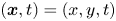$(\boldsymbol {x}, t)=(x,y,t)$ represents the spatial and time coordinates, $\boldsymbol {u}=(u, v)$ the velocity vector, $\rho _0$ the reference density, $p$ the pressure, $\nu$ the kinematic viscosity, $\boldsymbol {g}=(g_x,0)$ the gravity, $\beta$ the thermal expansion coefficient, $T$ the temperature, $k$ the thermal conductivity and $c$ the specific heat capacity. The mathematical symbols of $\boldsymbol {\nabla }\boldsymbol {\cdot }$, $\boldsymbol {\nabla }$ and $\varDelta$ are, respectively, the divergence, gradient and Laplace operators in the particular coordinate system being used. The Boussinesq approximation is justified if $\delta \rho =\beta \delta T=\beta (T-T_c) \ll 0.1$ (Chang & Sa Reference Chang and Sa1990), which is satisfied for all cases in the present study.

For the current flow configuration, the no-slip zero velocity and constant hot temperature ($T_h$) boundary conditions are applied to the rigid surfaces of the cylinders. The shear-free and adiabatic conditions are applied to the vertical channel walls. The coolant with temperature $T_c< T_h$ flows from the inlet face of the channel with a uniform velocity $(U_\infty,0)$. The outlet face of the channel is assumed to be an open boundary with zero velocity and temperature gradients. The pressure is prescribed to be zero at the outlet and zero gradients at the other boundaries.

Using the variables

(2.2a–f)\begin{align} \boldsymbol{u^{*}} = \frac{\boldsymbol{u}}{U_{\infty}},\quad x^{*} = \frac{x}{D}, \quad y^{*}=\frac{y}{D}, \quad t^{*} = \frac{tU_{\infty}}{D}, \quad p^{*} = \frac{p}{\rho U_{\infty}^{2}}, \quad T^{*} = \frac{T-T_c}{T_h-T_c} , \end{align}

equations (2.1) can be expressed in dimensionless forms as

(2.3a)$$\begin{gather} \boldsymbol{\nabla}\boldsymbol{\cdot} \boldsymbol{u^{*}} = 0 , \end{gather}$$

(2.3b)$$\begin{gather}\frac{\partial u^{*}}{\partial t^{*}}+\boldsymbol{u^{*}}\boldsymbol{\cdot} \boldsymbol{\nabla} u^{*} ={-} \boldsymbol{\nabla} P^{*} + \frac{1}{Re} \Delta u^{*}+ Ri\,\theta, \end{gather}$$

(2.3c)$$\begin{gather}\frac{\partial v^{*}}{\partial t^{*}}+\boldsymbol{u^{*}}\boldsymbol{\cdot}\boldsymbol{\nabla} v^{*} ={-} \boldsymbol{\nabla} P^{*} + \frac{1}{Re} \Delta v^{*}, \end{gather}$$

(2.3d)$$\begin{gather}\frac{\partial \theta}{\partial t^{*}}+\boldsymbol{u^{*}} \boldsymbol{\cdot}\boldsymbol{\nabla} \theta = \frac{1}{RePr}\Delta \theta . \end{gather}$$

The supscript $^{*}$ of the non-dimensional variables is omitted for simplicity for the rest of the paper. Equations (2.3) show that the governing parameters are $Ri$, $Re$ and $Pr$, which are defined as

(2.4a–c)\begin{equation} Re = \frac{U_{\infty}D}{\nu},\quad Ri = \frac{g\beta (T_h-T_c)D}{U_{\infty}^{2}},\quad Pr = \frac{\mu c}{k}, \end{equation}

respectively. In the present study, the investigated range of $Ri$ is from 0 to 1 to observe the gradual variation of behaviours with increasing buoyancy from forced convection. The upper limit of $Ri = 1$ is used because it can present large effects of buoyancy for flow around a solid cylinder (Hu & Koochesfahani Reference Hu and Koochesfahani2011). Here $Re$ is fixed at 100 since it is a typical value for laminar flow around a solid cylinder with vortex shedding; $Pr$ is fixed at 7 for water.

Due to the unsteady nature of the velocity and temperature fields, it is useful to analyse the mean flow and heat transfer characteristics. The time averaged, fluctuating and root mean square (r.m.s.) of the variable $\psi$ are defined as

(2.5a–c)\begin{equation} \bar{\psi} = \frac{1}{t_2^{*}-t_1^{*}}\int^{t_2^{*}}_{t_1^{*}} \psi \,{\rm d}t, \quad \psi' = \psi - \bar{\psi} , \quad \psi'_{rms} = \sqrt{\frac{1}{t_2^{*}-t_1^{*}}\int^{t_2^{*}}_{t_1^{*}} (\psi-\bar{\psi} )^{2} \,{\rm d}t}, \end{equation}

respectively. The $(t_2^{*}-t_1^{*})$ is the time duration of the flow in the saturated (fully developed) state. For flow within the array, the Eulerian-averaged variable is calculated as

(2.6)\begin{equation} \langle\bar{\psi}\rangle = \frac{1}{V_a(1-\phi)} \int_{V_a(1-\phi)} \bar{\psi} \,{\rm d}V , \end{equation}

where $V_a$ is the volume/cross-sectional area of any arbitrary representative area of the array.

For force analyses, the total drag and lift coefficients ($C_D$ and $C_L$) of the array are calculated from the sum of the forces exerted on the individual circular cylinder as

(2.7a,b)\begin{equation} C_D = \frac{\displaystyle\sum\limits_{i,\,j=1}^{N} \boldsymbol{F_{ij}}\boldsymbol{\cdot} \boldsymbol{\hat{x}}}{1/2\rho U^{2}_{\infty} D}, \quad C_L = \frac{\displaystyle\sum\limits_{i,\,j=1}^{N} \boldsymbol{F_{ij}}\boldsymbol{\cdot} \boldsymbol{\hat{y}}}{1/2\rho U^{2}_{\infty} D}, \end{equation}

where $i$, $j$ are the labels of each cylinder in the $x$ and $y$ directions, respectively; $\boldsymbol {\hat {x}}$ and $\boldsymbol {\hat {y}}$ are the unit vector in the horizontal and vertical directions, respectively. The force on the cylinder $(i,j)$ is expressed as $\boldsymbol { F_{ij}} = \int _{S_{c,ij}}(p\boldsymbol {I}-\boldsymbol {\tau })\boldsymbol {\cdot } \hat {\boldsymbol {n}} \,{\rm d} S_c$, where $\boldsymbol {\tau }$ is the stress tensor, $\boldsymbol {I}$ the identity matrix, ${S_{c,ij}}$ the surface of the cylinder ($i, j$) and $\hat {\boldsymbol {n}}$ the unit surface normal vector of the cylinder. Both $C_D$ and $C_L$ can be decomposed into the pressure and viscous force contributions. The drag coefficient of an individual cylinder is calculated as $C_{dij}=\boldsymbol {F_{ij}}\boldsymbol {\cdot } \hat {\boldsymbol {x}}$. The mean drag coefficient of an individual cylinder ($\overline {C_{dij}}$), the mean drag coefficient of the array ($\overline {C_D}$) and the r.m.s. lift coefficient (${C_L}_{rms}'$) for the array are calculated from (2.5a–c). The Strouhal number ($St$) is calculated as $fD/U_{\infty }$ with $f$ the frequency of the global fluctuating flow including the vortex shedding behind the array.

For heat transfer analyses, the Nusselt number of the array is calculated from the sum of the local Nusselt number of an individual cylinder as

(2.8)\begin{equation} Nu = \sum_{i=1}^{N} (Nu_{dij})= \sum_{i=1}^{N} \left[ \int_{S_{c,ij}} \left(-\frac{\partial T^{*}}{\partial n} \right) {\rm d} S_c \right ] , \end{equation}

where $\partial /\partial n$ is the gradient in the direction normal to the surface. The local Nusselt number ($Nu_d$) is calculated from $-(\partial T^{*}/\partial n)$, which is derived from the equation $k\partial T/\partial n = h(T_h-T_c)$ with $h$ being the local heat transfer coefficient. The mean local Nusselt number ($\overline {Nu_d}$), the mean Nusset number of an individual cylinder ($\overline {Nu_{dij}}$) and the mean Nusselt number of the array ($\overline {Nu}$) are calculated from (2.5a–c).

In the present study, the pressure implicit with splitting of operators scheme (Issa Reference Issa1986) is used to treat the pressure-velocity coupling in the numerical framework of the finite-volume method. The convection and diffusion terms in both momentum and energy equations are discretized by the second-order upwind method. The time derivative is discretized by a second-order method. All calculations are carried out in parallel with the message passing interface method. Verification and validation tests are performed for both an individual circular cylinder and an array of cylinders (including $\phi =1$), the details of which are presented in the Appendix section.

3.1. The mean recirculation regions

The recirculation behaviours are more complicated than those of the previous studies (e.g. Sharma & Eswaran Reference Sharma and Eswaran2004; Hu & Koochesfahani Reference Hu and Koochesfahani2011) on opposing-buoyancy mixed convection around a solid cylinder due to the geometrical effects of cylinder arrays. Based on the existence of different types of mean recirculation, six flow patterns (from P-1 to P-6) are identified, as indicated in figure 2.

Figure 2. $(a)$ Flow patterns based on mean recirculation regions in the parameter space of $Ri$ and $\phi$: P-1 represents symmetric flow (SF) with near-wake vortexes (NV); P-2 represents unsymmetric flow (UF) with NV; P-3 represents UF with NV and lateral vortexes (LV); P-4 represents UF with NV, LV, and detached far-wake vortexes (FV); P-5 represents UF with NV, LV and connected FV; P-6 represents UF with NV, LV, connected FV, and a small vortex pair between LV and NV. $(b)$ Sketch of P-4.

Pattern P-1 represents symmetric flow with one vortex pair in the near wake. A typical case of P-1 is shown in figure 3(a,g,m). A region with negative velocity is shown behind the rear of the array, indicating the existence of the alternating vortex with a similar size to that of the region. Figure 2(a) shows that, for $Ri=0$, all cases with different geometric configurations present the P-1 pattern. As $Ri$ increases, the symmetry only remains for larger $\phi$ cases, which indicates that the wake flow is less affected by the buoyancy force for larger $\phi$.

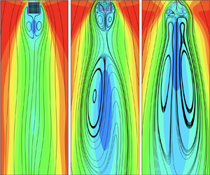
Figure 3. Plots of $u$-component velocity contours and streamlines for the (a–f) instantaneous flow field, (g–l) time-averaged flow field and (m–r) the near-wake region. Left to right: representative cases for patterns 1–6. The arrows in (q) and (r) indicate the local mean flow direction.

The corresponding temperature contours are presented in figure 4(a,g). The heat is carried away from the array via hot ‘blobs’ shedding from the two sides of the array, demonstrating ‘Kármán’ vortical structures. When the inertial flow penetrates into the array, the fluid is slowed down due to the blockage effect of the cylinders and part of it is redirected out the array from the lateral sides. If $Ri>0$, the upward buoyancy-induced flow further slows down the inertial flow and more fluid bleeds from the lateral sides. Note that the fluid is heated up when it moves in the array. Meanwhile, the surrounding flow is also heated up when it moves along the heated ‘porous wall’. The heated lateral bleeding flow, together with the heated surrounding flow, forms the thermal layer (TL) on the lateral sides of the array. In figure 4(g) the heat is almost locked by the compact cylinders within the array and the TLs develop along the lateral sides of the array, similar to that of a solid square cylinder.

Figure 4. Temperature contours for the (a–f) instantaneous flow and (g–l) time-averaged flow in the near-wake regions. Left to right: representative cases for patterns 1–6.

Pattern P-2 indicates the onset of unsymmetrical flows. Specifically, P-2 presents an unsymmetrical flow with one vortex pair, as shown in figure 3(h,n), which only appears when both $\phi$ and $Ri$ are small. The P-2 pattern indicates that the flow in the far wake begins to be disturbed due to the pore effects even though the buoyancy is small. The wake behind the array becomes wider with decreasing $\phi$. The widened wake is accompanied by more intense fluctuations further downstream, as demonstrated by the more curved streamlines. The streamlines in the far wake deviate from symmetry, where a region with almost zero velocity appears. Part of the fluid bleeds from the rear of the array, which is called the based bleed. The near-wake vortex pair is detached from the rear of the array due to the base bleed. The wake length becomes shorter, indicating that the alternating vortex rolls closer to the cylinder.

For P-2 (figure 4b), more heat is transported downstream compared with P-1 (figure 4a), indicating a larger overall heat transfer rate. The alternating shedding of hot ‘blobs’ also spans a wider space in the far wake, which contributes to the flow with more intense fluctuations. Figure 4(h) shows that the inertial flow promotes heat transfer in the upstream side of the array. A fairly large amount of heat is still locked in the array because of the blockage of cylinders and the buoyancy. The TLs on the lateral sides are much thicker than those of P-1 due to the enhanced interaction between the inertial flow and the buoyancy-induced reverse flow. The fluid, which is squeezed out from the lateral sides, seems to increase the effective frontal area of the bluff body. This expanded effective frontal area sheds light on the wider wake flow and lower shedding frequency.

Pattern P-3, as shown in figure 3(i,o), also indicates the onset of unsymmetrical flows when both $\phi$ and $Ri$ are relatively large. The lateral vortex pair is formed due to the relatively stronger reverse flow driven by upward buoyancy at larger $Ri$. Different from P-2, the asymmetry of P-3 is mainly caused by a large buoyancy force. For relatively large $Ri=0.75$ and $\phi =0.66$, the flow slightly deviates from symmetry with one vortex pair in the near wake, similar to that shown in figure 3(h). Patterns P-2 and P-3 indicate that the unsymmetrical region with almost zero velocity in the far wake can be caused by either large opposing buoyancy or porous effects. For relatively large $Ri=0.75$, an additional vortex pair appears on the lateral sides of the array due to stronger buoyancy-induced reverse flow. Besides, the similar flow patterns shown in figure 3(b,c) indicate that either a larger $Ri$ or a smaller $\phi$ gives rise to a wider wake.

At $Ri=0.75$, the shedding pattern of a compact array (figure 4c) is fairly similar to that of figure 4(b) except that the temperature of vortexes in figure 4(c) is much lower, implying a smaller heat transfer rate from the array. This also corresponds to a similar streamline pattern but somewhat less unsymmetric flow for $\phi =0.66$ (figure 3i) compared with figure 3(h). Based on the heat transported downstream, the heat transfer rates indicated in figure 4(a,c) are expected to be similar. Note that P-2 and P-3 form a qualitative bifurcation region dividing the symmetric and strongly unsymmetrical flows. The corresponding $Ri$ of the bifurcation region increases with $\phi$. Comparing P-1 and P-3, the larger buoyancy promotes a stronger reversed flow on the lateral sides of the array, forming the lateral vortex that thickens the TLs and prevents the heat from transferring downstream to some extent. Comparing P-2 and P-3, the alternating vortexes shedding from the array have similar width, but less heat is transferred downstream for P-3 since the lateral squeezing fluid is hindered by the higher resistance of the dense array in P-3.

Pattern P-4 represents an unsymmetrical flow with two vortex pairs and a detached recirculation region further downstream, a typical case of which is demonstrated in figure 3(d,j,p). The P-4 pattern also appears at $\phi =1$ and $Ri=1$ for a solid square cylinder (figure 2a). The discontinuity from a very compact array to the solid square cylinder results from the difference between the shape of the two bodies, which was also observed in the previous study (Tang et al. Reference Tang, Yu, Shan, Li and Yu2020, Reference Tang, Yu, Shan, Chen and Su2019). Similarly, at fixed $Ri=0.75$ (figure 3c–f) the streamlines become more curved and the wake becomes increasingly wide as $\phi$ decreases from 0.66 to 0.0079. The instantaneous velocity contours show that the near-wake negative velocity region of P-4 is shorter compared with P-3; also, a small vortex begins to appear in the far wake. Figure 3(o,p) also shows that the near-wake mean closure length decreases as $\phi$ decreases. The temperature contours of P-4 in figure 4(d) show a wider distance between alternating shedding vortexes and a higher temperature of the hot ‘blobs’ compared with P-3. The TLs are thicker owing to more heated flow exiting the array from the lateral sides.

We note that the present results are consistent with the previous experimental results. For a solid circular cylinder under opposing buoyancy at relatively large $Ri\geqslant 0.72$, the experiments of Hu & Koochesfahani (Reference Hu and Koochesfahani2011) showed that small ‘Kelvin–Helmholtz’ (KH) vortexes concurrently shed in the near wake of the heated cylinder, which would merge to form larger vortex structures further downstream. Here, the small vortexes are not observed, instead, the large vortex sheds alternately at the two lateral sides of the heated square cylinder or cylinder array for all $Ri$. This is because the flow shown here is in the recurrent stage, and the experimental results (Hu & Koochesfahani Reference Hu and Koochesfahani2011) are obtained at an earlier stage of the flow evolution, showing KH instability. Although the KH vortexes are not apparent in the recurrent stage, the instability indicated in the early stage of the evolution should be the same instability that causes the fluctuating velocity downstream, as will be discussed later for figure 7. As $\phi$ decreases, this instability increases and, therefore, results in a larger velocity deficit in the far wake.

Pattern P-5 is an unsymmetrical flow with connected near-wake and far-wake vortexes, which occurs at small $\phi$ under large $Ri$, as observed in figure 3(e,k,q). The superposition of pore effects and buoyancy gives rise to a more disturbed flow. The instantaneous streamlines (figure 3e) show that the near-wake negative velocity region is much larger than that of a larger $\phi$ case. An enlarged vortex is closely attached to the rear of the near-wake vortex with a different rotating direction. Also, the size and number of the vortexes in the far wake increase due to more complex flow interactions. The time-averaged streamlines (figure 3k) show that the near-wake vortexes are ‘engulfed’ into the large recirculation downstream. It is clearly seen in the near wake (figure 3q) that the lateral vortexes penetrate the more sparse array.

Figure 4(e,k) presents the corresponding temperature contours for P-5. The width of the vortex shedding is evidently larger and the frequency of vortex shedding is smaller than those of patterns 1–4, consistent with the instantaneous velocity contours shown in figure 3. The mechanism of this phenomenon lies in the interaction of buoyancy-induced flow and inertial flow. With a smaller $\phi$, the permeability of the array is larger. Thus, the downward inertial flow and the upward buoyancy-induced flow can easily penetrate the array and squeeze more hot flow out of the lateral sides, forming thicker TLs. The thickened TLs expand the effective frontal area, which causes the decrease of the shedding frequency and enlargement of the width of the wake.

Pattern P-6 is similar to P-5 except that another vortex pair appears between the lateral and the near-wake vortexes, as seen in figure 3(l,r). The small vortex pair is mainly caused by the compromise between the bleeding flow from the array and the much larger surrounding (lateral and the near-wake) vortexes. Similar small vortexes were also observed by Sharma & Eswaran (Reference Sharma and Eswaran2004) at $Ri=0.5$ and $Pr=0.7$, which are attached to the rear side of the array due to the interaction of the buoyancy-induced flow and the vortexes behind the cylinder. The size of the connected near-wake and far-wake vortexes becomes smaller than that presented in figure 3(k) due to the smaller strength of the fluctuation in the far wake, as will be discussed for figure 7. The temperature contours in figure 4( f,l) show that more heat is convected downwards for P-6. For relatively small $\phi$, the frequency of vortex shedding at higher $Ri$ is smaller.

Note that patterns of P-4, P-5, P-6 on the upper side of the bifurcation region all present large recirculation further downstream, showing strong unsymmetrical behaviours. The interaction of the inertial flow and the buoyancy-induced reverse flow occurs within the array as well as on the lateral surfaces of the array. The interaction inside the array squeezes the fluid toward the lateral sides and thickens the TLs. The interaction on the lateral surfaces induces instability of the squeezed flow, which is transported downstream, forming detached vortices. The lateral bleeding flow becomes stronger with increasing $Ri$ and decreasing $\phi$. Meanwhile, the heat transfer rate from the bottom row of the cylinder array increases, also due to the enhanced buoyancy-induced reverse flow with increasing $Ri$ and decreasing $\phi$.

Figure 2(b) shows a sketch of the typical averaged flow structure, using P-4 as an example. Here $L_B$ is the distance between the rear of the array and the rear stagnation point of the near-wake vortexes; $L_C$ is the distance between the rear side and the farthest stagnation point on the centreline no matter if the near wake is connected with the far wake or not. For cases without vortexes in the far wake, $L_C$ is taken to be the same as $L_B$. The distance between the rear of the array and the first saddle point in the centreline is denoted as $L_T$.

The flow structure is mainly determined by the interaction among the inertial flow, the buoyancy-induced reverse flow and the cylinder array. If the buoyancy-induced reverse flow and the block effect of the cylinder array are weak, part of the inertial flow passes through the array and then reaches a stagnation point downstream of the array. However, this stagnation point may be located within the array when $\phi$ and $Ri$ are relatively large. Thus, the penetration depth $L_P = D+L_T$, which reflects the location of the stagnation point, can be defined to quantitatively describe this interaction. The penetration depth is largely dependent on the strength of the penetrating inertial flow and the buoyancy-induced reverse flow at various $Ri$ and $\phi$. The tendency of variation of penetration depth with $Ri$ is similar to that shown by Goldman & Jaluria (Reference Goldman and Jaluria1986) for negatively buoyant flows.

Figure 5 shows the summary of the length of the vortex in the centreline. As shown in figure 5(a), $L_C$ can be very large for relatively high $Ri$ and/or low $\phi$. For the solid square cylinder, $L_C$ first decreases slightly and then increases to around $10.5D$, the tendency of which is consistent with the previous experimental results (Hu & Koochesfahani Reference Hu and Koochesfahani2011) for a solid circular cylinder. The $L_C$ at $\phi =0.42$ is fairly similar to that of the solid case, as indicated earlier in figure 2. It is observed that the $L_C$ at $Ri=1$ increases as $\phi$ decreases from 0.22 to 0.026. However, the $L_C$ at $Ri=1$ decreases when $\phi$ further decreases to 0.0079. The largest $L_C$ is ${\sim }25D$ for $\phi =0.026$ and $Ri=1$, which is more than twice as large as that of flow around a solid counterpart.

Figure 5. Variations of $(a)$ $L_C$, $(b)$ $L_B$ and $(c)$ $L_T$ with $Ri$ for different $\phi$.

Figure 5(b) shows the variation of $L_B$ with $Ri$. For $\phi \geqslant 0.22$, $L_B$ first increases and then decreases with $Ri$. The decreasing trend is consistent with that of Sharma & Eswaran (Reference Sharma and Eswaran2004). The $L_B$ at $\phi =0.66$ is quite similar to that of the solid case, while the $L_B$ at $\phi =0.22$ is evidently smaller than those of the compact array cases. For small $\phi \leqslant 0.063$, $L_B$ is obtained only at relatively small $Ri$ when the near-wake and far-wake vortexes are separated. The $L_B$ at $\phi =0.026$ follows the trend of the larger $\phi$ cases though it is noticeably smaller. Unexpectedly, the variation trend of $L_B$ at $\phi =0.063$ is opposite to those at $\phi \geqslant 0.22$, but is consistent with that of $\phi =0.0079$. This is actually due to the balanced effects of the base bleed and the fluctuating intensity of the flow since the base bleed distance is included in $L_B$. For $\phi =0.063$ and $0.0079$, the base bleed is much larger than those of the compact array cases, resulting in larger $L_B$. For $\phi =0.026$, although the base bleed is also large, the mean vortex is much shorter due to the faster shedding of vortexes. Overall, $L_B$ for small $\phi$ does not vary much with $Ri$, which ranges from approximately 2 to 2.4.

Figure 5(c) shows the variation of $L_T$ with $Ri$. For large $\phi =0.66$, the magnitude of $L_T$ increases monotonically with $Ri$ and $L_P$ decreases correspondingly since the buoyancy force is comparably larger than the inertial flow within the compact array. For $\phi =0.22$, $L_T$ slightly deviates from those of larger $\phi$ cases. The $L_T$ at $\phi \leqslant 0.063$ is positive for small $Ri$ since the array allows more inertial flow to go through it; $L_T$ is negative at larger $Ri$ since the reverse flow becomes strong, which penetrates through the array from the bottom.

Figure 6 shows a summary of the length of the lateral vortex pair, which is mainly formed by the interaction of upward buoyancy and downward inertial flow. In the present work, the lateral vortex pair only occurs for $Ri\geqslant 0.5$. This indicates that the large reverse flow induced by buoyancy is the main factor promoting the formation of the lateral vortexes. Also, the lateral vortex pair occurs at a smaller $Ri$ when $\phi$ is smaller, demonstrating that a certain pore structure of the array can promote the formation of the lateral vortexes. Figure 6 demonstrates variations of the relative positions of the lateral vortex core ($C_X, C_Y$) and the saddle point ($S_X, S_Y$) with $\phi$ at different $Ri$. Figure 6(a) shows that the absolute values of $C_Y$ increase with $Ri$, indicating that the vortex core moves upward along with increasing buoyancy. For fixed $Ri$, $C_Y$ first decreases, then increases and finally decreases with an increment of $\phi$, which is due to the competence of the inertial flow and the buoyancy-induced flow under porous effects. On the other hand, $S_Y$ does not change much across the range of $\phi$ for different $Ri$, which is $\sim$0.2.

Figure 6. Variations of $(a)$ $C_Y$, $S_Y$ and $(b)$ $C_X$, $S_X$ with $\phi$. $(c)$ Illustration of the lateral and near-wake vortexes.

Contrastingly, figure 6(b) shows that $C_X$ does not change much with $\phi$ and $Ri$, which is approximately 0.75, while $S_X$ differs much with both parameters, especially at small $\phi$. The variation of $S_X$ with $\phi$ shows a fluctuating trend due to the more complicated wake behaviours, e.g. the appearance of an additional vortex pair between the lateral and near-wake vortexes. Overall, $S_X$ at smaller $\phi$ is shorter, which implies that the vortex size is larger. In addition, the lateral vortexes are largely related to the TLs on the two sides of the array, as demonstrated by the mean temperature in figure 4. The forced inertial flow develops a downward viscous layer on the array surface, which comes across the upward viscous layer formed by the buoyancy-induced reverse flow, resulting in an enclosed zone with heat kept inside and a recirculation formed beneath it. The enclosed zone is wider for smaller $\phi$ because of the lateral bleeding of the heated flow.

We next present more analyses on the transition behaviours between different flow patterns. The transition between P-1 and P-2 mainly occurs at relatively small $0.0079<\phi <0.1$ and $0< Ri<0.25$ since the evident upward buoyancy within the array causes a small instability in the far wake. For relatively large $0.1<\phi <1$ and $0.25< Ri<0.5$, the flow pattern transits from P-1 to P-3 due to the buoyancy-induced flow separation on the lateral sides of the array. The transition from P-3 to P-4 occurs at relatively large $0.1<\phi <0.56$ and $0.5< Ri\leqslant 1$ since the instability in the far wake increases, forming vortexes, with increasing buoyancy effects. The flow can also transit directly from P-2 to P-4 at $0.026<\phi <0.1$ and $0.25< Ri<0.5$, indicating that a porous medium promotes instability even at moderate buoyancy force. The flow transits from P-4 to P-5 at $0.026<\phi <0.1$ and $0.5< Ri\leqslant 1$ because the area with strong instability further increases in the far wake, causing connection of the near- and far-wake vortexes. Note that at $\phi =0.0079$, P-2 directly transits to P-5 due to the large pore effects on the instability downstream. The mechanism that leads to the far wake is related to the fluctuations. The fluctuations are caused by the instability triggered by the upward buoyancy-induced reverse flow and the downward inertial flow. With the increments of the countercurrent flow, more unsteady structures are formulated on the lateral surfaces, which move downstream and form larger detached vortices behind the array.

As indicated above, the fluctuations caused by the instability play an important role in the far-wake behaviour. Therefore, a detailed discussion on the instability indicated by the fluctuating kinetic energy (FKE) and the fluctuating heat flux (FHF) is provided below. Here, FKE is calculated from $0.5\times [(u_{rms}')^{2}+(v_{rms}')^{2}]$. Figure 7 shows distributions of mean velocity deficit (MVD) (a–f) and FKE (g–l) at various $Ri$ and $\phi$. Here, MVD is calculated as $(U_{\infty }-\bar {u})/U_{\infty }$. The flow pattern based on figure 2 is indicated on the left corner of each MVD figure. The distance between the rear of the array and the bottom boundary of the figure is $23D$ and $47D$ for MVD and FKE, respectively.

Figure 7. Distributions of the mean velocity deficit (MVD) (a–f) and the fluctuating kinetic energy (FKE) (g–l) for different $Ri$ and $\phi$ as indicated.

For relatively large $\phi =0.22$ (figure 7a–c,g–i), the region with ${\rm MVD}\geqslant 0.2$ becomes larger with an increment in $Ri$. Correspondingly, the region with ${\rm FKE} \geqslant 0.044$ also enlarges evidently with increasing $Ri$. At $Ri=0$ (figure 7a,g), the region with high MVD values mainly exists right behind the rear of the array, where a vortex pair is formed. It is seen that FKE in the region of the near-wake vortex is very small. The largest FKE appears behind the vortex region. At $Ri=0.5$ (figure 7b,h), two local maximums of MVD appear at the near-wake and far-wake regions, respectively, though no vortex is actually formed in the far wake (P-3 pattern). The FKE in the region of the near-wake vortex is also very small, which increases and reaches a local maximum at approximately $23D$ downstream of the array. The local maximums of MVD and FKE appear in roughly the same area. At $Ri=1$ (figure 7c,i), the local maximums of MVD move further upstream. The distance between the local maximums is also smaller. Pattern P-4 indicates that the large recirculation is formed in the far wake, which is detached from the near-wake vortex. In this case, a local maximum of FKE occurs in the region between the near- and far-wake vortexes, indicating that the locally strongest fluctuation occurs when the flanks of the two contra-rotating vortexes clash with each other. Also, a local maximum of FKE appears further downstream due to the energy cascade from the detached vortexes.

For relatively small $\phi$ (figure 7d–f,j–l), the region with large MVD is evidently larger, especially for mixed convection. The fluctuations are also much more intense, especially for $Ri=1$. The local maximum of FKE also moves further downstream for smaller $\phi$. Overall, the large recirculation zone in the far wake is well correlated with FKE. For moderate fluctuating intensity, the recirculation region is detached from the near-wake vortex. As FKE increases, the recirculation region becomes larger. Once the recirculation enlarges to a certain size, it comes across the near-wake vortex and connects as well as develops with it. This also indicates that the formation mechanisms of the near-wake and far-wake vortexes are different. The near-wake vortex mainly results from flow separation from the extended shear layer formed by the bleeding flow from the rear of the array and the surrounding fluid flow on the lateral sides of the array, while the far-wake vortexes are somewhat related to the fluctuations from the instabilities developed from the interaction of the opposing buoyancy with the inertial flow, which is intensified by the porous matrix of the array.

The variations of MVD and FKE with the streamwise distance along the centreline are also presented in figure 8. The region with MVD greater than 1 indicates the formation of vortexes. Figure 8(a) shows that, under forced convection, MVDs are almost the same for all the presented cases for $x/D\leqslant 3$, which is the length of the near-wake vortex. The decreasing rate of $\phi =0.0079$ is relatively small. Correspondingly, FKE is larger as $\phi$ decreases though FKE does not differ much among all $\phi$ cases.

Figure 8. Variations of (a–c) MVD and (d–f) FKE with $x/D$ for (a,d) $Ri=0$, (b,e) $Ri=0.5$ and (c, f) $Ri=1$.

As $Ri$ increases to 0.5 (figure 8b), the difference among various $\phi$ is obvious. For $\phi =0.66$, MVD is similar to that of forced convection except that MVD in the far wake is still much larger than that of $Ri=0$. The maximum value of FKE occurs at approximately $x/D=9$. For $\phi =0.22$, a secondary velocity deficit (bump) occurs at $x/D\sim 11$, but the vortex is not literally formed since the maximum value of the second bump is ${\sim }1$. The variation trend of the corresponding FKE is also similar to that under forced convection but the value of FKE is much larger. For smaller $\phi \leqslant 0.026$, MVD is presented with two local maximums (two bumps), both of which are noticeably larger than 1, indicating the formation of vortexes. The FKE also shows two bumps in these cases. Overall, the present results are consistent with those of the previous study (Hu & Koochesfahani Reference Hu and Koochesfahani2011) since both studies indicate a large MVD region behind the body at large $Ri$. However, the current results show that the velocity can recover up to around 0.1 before the secondary deficit while the velocity reported by Hu & Koochesfahani (Reference Hu and Koochesfahani2011) is almost zero. Also, the present study shows that the velocity deficit does not always indicate a recirculation downstream. The differences partially come from the different stages of flow investigated in the two studies.

For $Ri=1$, the decreasing rates of MVD with $x/D$ are much smaller compared with smaller $Ri$ cases. At $\phi =0.66$, MVD shows two bumps with the second one below 1, therefore, no vortex appears. The FKE also only has one peak. At $\phi =0.22$, the second velocity deficit region is much larger than the first one. The FKE shows two bumps with similar peak values. At smaller $\phi =0.026$, the recirculation in the far wake becomes much larger. It is observed that the local maximum of FKE for the second bump is the highest among all $\phi$ cases, which corresponds to the smallest decreasing rate of MVD. For $\phi =0.0079$, both FKE and MVD are noticeably smaller than the cases of $\phi =0.026$. Also, for $\phi =0.026$ and $0.0079$, only one peak is shown for MVD due to the connection of the near-wake and far-wake vortexes. However, FKE still shows two bumps, indicating that it is actually two types of vortexes.

Apart from this, the FHF is also calculated since the intense FKE in the far wake is considered to be transported from the lateral sides of the array, where FHF is strong. The FHF is calculated as $\sqrt {(\overline {u'T'})^{2}+(\overline {v'T'})^{2}}$, where the fluctuating velocity and temperature are obtained at the same time. Figure 9 shows the distributions of FHF for various $Ri$ and $\phi$. For $\phi =0.22$ and $Ri=0$, two regional pairs with local maximums of FHF are shown in the near wake of the array. The smaller regional pair is on the lateral sides of the larger regional pair. As $Ri$ increases, the regional pair on the lateral sides moves upstream and becomes much larger, while the regional pair in the middle becomes noticeably smaller. The distance between each pair of regions is also larger. The trend is more obvious at $Ri=1$, where the local maximum of FHF in the lateral regional pair is much higher than those of smaller $Ri$ cases. The instability caused by FHF mainly develops on the lateral sides of the array and accumulates as the fluid flows downstream. For relatively small FHF, the instability transported downstream is not sufficiently strong to form a large recirculation (figure 9b). For larger FHF, the accumulated instability promotes the formation of large recirculation in the far wake. If the accumulation takes a much longer distance than the length of the near-wake vortexes, the large recirculation would be detached from the near-wake vortexes, which is the situation for figure 9(c).

Figure 9. Distribution of FHF for different $Ri$ and $\phi$ as indicated.

For relatively small $\phi =0.026$, the distributions of FHF undergo similar changes with an increment of $Ri$, except that the regional pairs are much larger compared with the case of $\phi =0.22$. Also, an additional regional pair is presented behind the array for $Ri=0.5$ due to the pore effects of the array, which promotes the formation of detached recirculation downstream. For $Ri=1$, the lateral instability caused by large FHF is also large, which requires less distance for accumulation, so the large recirculation can be formed more upstream of the array. This also indicates that the large recirculation is easier to interact with the near-wake vortexes within such a short distance. The analyses are also consistent with the observations made by Hu & Koochesfahani (Reference Hu and Koochesfahani2011), where the KH-like small vortex structures shed on the two sides of the circular cylinder, which would merge to form larger vortex structures further downstream. The merging process was found to be similar to the ‘pairing’ process of ‘KH’ vortex structures in a free shear layer. As already indicated in the last section, the phenomenon observed by Hu & Koochesfahani (Reference Hu and Koochesfahani2011) might be from an earlier stage of the flow. Here, although KH vortexes were not observed, their effects are still accumulated and would contribute to the formation of the large recirculation further downstream.

The mean flow on the lateral sides of the array is closely related to FHF. Figure 10 shows the mean $u$-component velocity and the corresponding FHF profiles with respect to $y/D$ at fixed $x=D$. The lateral surface of the array is at $y/D=0$. For $Ri=0$ (figure 10a,d), drastic changes of both $\bar {u}$ and FHF occur at $y/D\lesssim 0.6$. For the presented $\phi$, $\bar {u}$ first increases to a maximum value and then decreases gradually to the free-stream velocity with $y/D$, similar to that of flow around a solid cylinder. For fixed $y/D$, $\bar {u}$ decreases as $\phi$ decreases though the difference among the presented $\phi$ is small. In the range of $y/D\lesssim 0.6$, FHF first increases rapidly to a maximum value and then decreases sharply to zero. The maximum value of FHF as well as the range of $y/D$ with non-zero FHF increase with decreasing $\phi$. This indicates that the porous lateral surface with flow injection promotes fluctuating intensity. Overall, FHF does not have large effects on $\bar {u}$ since FHF is relatively small with ${O}(10^{-3})$.

Figure 10. Variations of (a–c) the mean velocity and (d–f) the FHF with $y/D$ at fixed $x=D$ for (a,d) $Ri=0$, (b,e) $Ri=0.5$ and (c, f) $Ri=1$. The BLE solutions are obtained at $\phi =0.0079$.

The mean $u$-component velocity profiles at very small $Ri$ are also similar to those presented in figure 10(a). For these cases, the boundary layer thickness is much smaller than the side length of the array; therefore, the flow behaviour is expected to be similar to that of flow over a flat plate and the flow can be described by the simplified equations of the boundary layer flow (BLF) as

(3.1a)$$\begin{gather} u\frac{\partial u}{\partial x} + v\frac{\partial u}{\partial y} =\nu \frac{\partial^{2} u}{\partial y^{2}}- g\beta (T-T_c), \end{gather}$$

(3.1b)$$\begin{gather}u \frac{\partial T}{\partial x} + v\frac{\partial T}{\partial y} = \alpha \frac{\partial^{2} T}{\partial y^{2}} , \end{gather}$$

with the divergence condition. The equations were demonstrated to be applicable for forced convection as well as mixed convection with aiding buoyancy (Makinde & Olanrewaju Reference Makinde and Olanrewaju2010). Equations (3.1) can be transferred to the simpler ordinary differential equation (ODE) by using the similarity variable method. The coupled ODE can then be solved by using the shooting method. Preliminary calculations for forced and mixed convection with very small opposing buoyancy are performed. The BLE velocity profile at $Ri=0.25$ and $\phi =0.0079$ is presented in figure 10(a), which is similar to the numerical results under forced convection, except for the velocity far away from the lateral surface due to the difference between a real flat plate and a bluff body.

With the effects of larger opposing buoyancy (figure 10b,e), the differences in the $\bar {u}$ and FHF profiles among various $\phi$ are much larger. In the region close to the lateral surface (inner region), $\bar {u}$ either increases with a much smaller rate or varies non-monotonically with $y/D$ compared with that under forced convection due to the diffusion caused by the reverse flow and the lateral vortex. The FHF in the inner region is relatively small (${\lesssim }0.01$). In the region further away from the lateral surface (outer region), $\bar {u}$ increases drastically with $y/D$. The corresponding FHF also varies tremendously with $y/D$. It is seen that $\bar {u}$ decreases with decreasing $\phi$ for $\phi \leqslant 0.026$, but then increases as $\phi$ further decreases to 0.0079. This is also reflected in figure 10(e), where the maximum FHF is observed for $\phi =0.026$. The value of FHF also becomes much larger with opposing buoyancy. For small $\phi$, the maximum $\bar {u}$ is no greater than the free-stream velocity since part of the fluid flows through the array. The range of $y/D$ with non-zero FHF also extends to approximately 1.5.

For even larger $Ri=1$ (figure 10c, f), the variation trends observed at $Ri=0.5$ are more obvious. The inner region becomes larger due to the growing size of the diffusing vortex. The corresponding FHF is also small in this region. In the outer region the maximum $\bar {u}$ for all $\phi$ becomes even smaller since more fluid flows through the array, which also indicates that the resistance of the array is smaller for larger $Ri$. The region with the largest variation of $\bar {u}$ and non-zero FHF also extends to $y/D=3$ for $\phi =0.0079$. Overall, the enhanced buoyancy and the porous matrix intensify the fluctuations.

Obviously, (3.1) cannot be directly applied to flow with relatively large opposing buoyancy due to the formation of lateral vortexes. However, the equations still produce reasonable results if the viscosity is modified with an appropriate value. For relatively large $Ri$, the whole domain can be divided into the inner region close to the boundary and the outer region for the rest of the domain. The variable at the interface is assumed to be known from the direct numerical simulation. The modified viscosity ($\nu _e$) in each region is determined from trial and error. It is seen in figure 3.1(b,c) that the BLF solutions agree well with the numerical results when $\nu _e$ is applied. For $Ri=0.5$, $\nu _e/\nu =$ 8 and 1.6 for inner and outer regions, respectively; for $Ri=1$, $\nu _e/\nu =$ 70 and 4 for inner and outer regions, respectively. In the trial and error process, $\nu _e$ is found to increase with increasing $Ri$ and/or decreasing $\phi$. Also, a more accurate estimation of $\nu _e$ is expected to follow the variation trend of FHF with $y/D$ (see figure 10e, f), i.e. $\nu _e$ first increases and then decreases with $y/D$, indicating that $\nu _e$ is highly related to the fluctuations. The modified viscosity mainly adds artificial dissipation to the flow, which is quite similar to the concept of eddy viscosity in turbulence modelling.

3.2. The force coefficients

The fluctuating force coefficients exerted on the whole array are considered in this section. Figure 11 shows the representative phase portraits of $C_D$ and $C_L$ at $\phi =0.0079$ and $Ri\geqslant 0.5$. The corresponding power spectra density (PSD) obtained from the time series of $C_L$ is also presented. At $Ri=0.5$ (figure 11a,d), the phase portrait presents a very narrow band of orbits similar to the limit cycles. The PSD shows a single sharp peak at $St=0.092$, indicating that it is still a periodic (P) flow. The $St$ for the peak amplitude depicts the frequency of vortex shedding of the near-wake vortexes. For $Ri=0.75$ (figure 11b,e), the phase portrait becomes more complicated with wide bands of cycling orbits. The corresponding PSD also shows some noisy power spectra surrounding the peak, presenting periodic (P*) behaviours that are different from those in figure 11(a,d). The phase portrait is even more complex for $Ri=1$ (figure 11c), presenting direct orbits from one ‘wing’ to the other. The PSD (figure 11f) shows distinctly three peaks with comparable amplitudes, which is denoted as quasi-periodic (QP).

Figure 11. Phase portrait (a–c) and PSD (d–f) at fixed $\phi =0.0079$ for (a,d) $Ri=0.5$, (b,e) $Ri=0.75$, (c, f) $Ri=1$.

The dynamic behaviours are closely related to the vortexes formed behind the rear side and on the lateral sides of the array. A summary of the flow behaviours is also provided in figure 12 for $Ri\geqslant 0.5$ and $\phi \leqslant 0.22$, along with the indications of flow patterns in the presented range of parameters. The dynamic behaviours for P-1, P-2 and P-3 are all periodic since the near-wake vortex shedding is the major cause of fluctuation. The behaviours in the P-4 region are also periodic because the large recirculation is detached from the near-wake vortex without influencing the dynamic behaviour of the integrated forces.

Figure 12. Power spectra density behaviours of the array-scale force coefficients, all other points are periodic.

In P-5 and P-6 regions, different types of behaviours are shown. For either smaller $Ri$ or larger $\phi$, the periodic behaviours are observed because the large recirculation is only weakly connected with the near-wake vortex and, therefore, has negligible effects on the periodicity (e.g. figure 11a,d). For larger $Ri\geqslant 0.75$, the P* behaviour occurs (e.g. figure 11b,e). This is because the large recirculation is moderately connected with the near-wake vortex, affecting the original vortex shedding mode to some extent. For $Ri=1$ at relatively small $\phi$, behaviours of noisy subharmonic and quasi-periodic appear. In this circumference, the large recirculation is strongly connected with the near-wake vortexes, which affects the integrated force with a different frequency. Also, large parts of the lateral vortexes penetrate the array, which gives rise to a third distinct peak of the PSD. Here, the difference between quasi-periodic and noisy subharmonic is due to the relative amplitudes of the three peaks. For noisy subharmonic, the subharmonic peaks due to the large recirculation and the lateral vortexes are evidently smaller than that of the fundamental peak; while for quasi-periodic, the subharmonic peaks are comparable to the fundamental peak.

As indicated above, the case with $\phi =0.0079$ and $Ri=1$ shows the most noisy behaviours for the investigated range of parameters. The observations also support the results and analyses in the previous study (Tang et al. Reference Tang, Yu, Shan, Li and Yu2020) that the critical $Re$ for the transition from steady to unsteady flow past a cylinder array is the smallest for $\phi =0.0079$, which is due to the interactions of inertial and viscous forces within the array. Here, the opposing buoyancy intensifies the interactions of forces between cylinders, which is expected to further decrease the critical $Re$. Although the noisy behaviour contributes to the triggering of unsteadiness, it does not necessarily result in large fluctuations as well as the large mean recirculation in the far wake. This is consistent with the observation that the largest recirculation downstream occurs at $\phi =0.026$ rather than $\phi =0.0079$ (figure 5a). The large recirculation in the far wake mainly results from a combined effect of the complexity and the amplitudes of the fluctuations.

Figure 13(a) shows the variation of ${C_L}_{rms}'$ with $Ri$ at different $\phi$. For $\phi =1$, ${C_L}_{rms}'$ increases with $Ri$, consistent with the previous study (Sharma & Eswaran Reference Sharma and Eswaran2004). The ${C_L}_{rms}'$ of $\phi =0.66$ are noticeably smaller than that of other $\phi$ for the investigated range of $Ri$. For an array with $\phi =0.22$, ${C_L}_{rms}'$ also increases monotonically with increasing $Ri$ but with much larger values. This is because the interacting forces in the array become more active, resulting in more intense fluctuations than the solid square cylinder. For $\phi =0.0079$, ${C_L}_{rms}'$ also increases with $Ri$, but with a trivial increment for larger $Ri$. The increasing rate declines when $Ri$ is larger. The variation trends are also similar to those of ${C_L}_{rms}'$ with $Re$ in the previous study (Tang et al. Reference Tang, Yu, Shan, Li and Yu2020). The variation trend of the fluctuation of $C_D$ with $Ri$ is also similar to that of $C_L$, thus not repeated here.

Figure 13. Variations of ${C_L}_{rms}'$ with (a) $Ri$ and (b) $\phi$.

The variations of ${C_L}_{rms}'$ with $\phi$ at fixed $Ri$ are presented in figure 13(b). For all $Ri$, ${C_L}_{rms}'$ decreases as $\phi$ decreases from 1 to 0.66, which implies that the compact array of circular cylinders with round corners could decline the intense fluctuations brought about by the sharp corners of the square cylinder. The discontinuity is also revealed in figure 2, where P-4 presents for both $\phi =1$ and 0.42 while P-3 presents for both $\phi =0.56$ and 0.66. For $\phi \leqslant 0.063$, ${C_L}_{rms}'$ decreases with decreasing $\phi$, showing a peak value of ${C_L}_{rms}'$ in the investigated range of $\phi$. This results from the changes in interacting force among the cylinders. As the distance between the cylinders becomes larger, the interaction changes from the viscous-force-dominated interaction to the inertial-force-dominated interaction, which decreases the coherent forces within the array.

The Strouhal number for the array-scale vortex shedding ($St_v$) is also investigated. For most cases, the flow is periodic so that the shedding frequency of vortexes is easy to detect. For certain cases with noisy behaviours (e.g. figure 11f), the frequency of the highest power is obtained. Figure 14(a) shows variations of $St_v$ with $Ri$ at different $\phi$. For ${\phi =1}$, $St_v$ decreases monotonically with increasing $Ri$, the trend of which is consistent with the previous studies (Chang & Sa Reference Chang and Sa1990; Sharma & Eswaran Reference Sharma and Eswaran2004; Hu & Koochesfahani Reference Hu and Koochesfahani2011). It is also observed that $St_v$ does not vary much among cases with $\phi \geqslant 0.22$. As $\phi$ decreases, the decreasing rate of $St_v$ with $Ri$ becomes larger. The minimum $St_v\approxeq 0.065$ is obtained at $\phi =0.0079$ and $Ri=1$. The decreasing trend of $St_v$ with either increasing $Ri$ or decreasing $\phi$ can also be observed from the instantaneous temperature fields (figure 4).

Figure 14. Plot of $St_v$ varying with (a) $Ri$ and (b) $Ri_{{eff}}$ for different $\phi$ as indicated.

Figure 14(b) shows that the $St_v$-$Ri_{{eff}}$ curves of all cases are almost collapsed into the same curve when $Ri$ is modified as the effective Richardson number ($Ri_{{eff}}$). For mixed convection around the solid cylinder, $Ri$ accounts for the buoyancy force induced by heat transfer from the cylinder surface. However, for the cylinder array, the effective $Ri$ should be considered due to the combined effects of the upward buoyancy-induced reverse flow within the array and the blockage effect of the array. Thus, the $Ri_{{eff}}$ can be regarded as the multiplication of a shape factor $r_s$ and $Ri$, with $r_s$ closely related to the $\phi$ of the array. For compact arrays with a large $\phi$, the combined effects are fairly small, i.e. $Ri_{{eff}}\approxeq Ri$. The permeability of the array increases as $\phi$ decreases. Thus, for the array with a relatively small $\phi$ or larger permeability, the upward buoyancy-induced reverse flow becomes stronger and the combined effects are much larger, i.e. $Ri_{{eff}}> Ri$. Here, the shape factor $r_s$ is estimated somewhat empirically. For $\phi \approxeq 1$, $r_s\approxeq 1$. For smaller $\phi$, $r_s> 1$. In the range of the investigated $Ri$ and $\phi$, the $r_s$ is found to satisfy a linear relationship,

(3.2)\begin{equation} r_s=Ri_{{eff}}/Ri={-}A_e\sqrt{\phi}+B_e\quad \text{for} \ \phi\leqslant 0.22, \end{equation}

with the coefficients of $A_e$ and $B_e$ being 3.69 and 3.02, respectively. The collapsed curve can be fitted into a polynomial relationship of $St_v =A_tRi_{{eff}}^{2}-B_tRi_{{eff}}+C_t$, where the coefficients of $A_t$, $B_t$ and $C_t$ are 0.0077, 0.0498 and 0.143, respectively. Besides, the collapsed curves with respect to $Ri_{{eff}}$ are only observed for $St_v$ rather than $\overline {C_D}$ and ${C_L}_{rms}'$. This is because $St_v$ is mainly dependent on the geometry while other parameters are not only dependent on the geometry but also the recirculating wake.

The mean drag coefficients exerted on the array of cylinders also carry important information on flow through the array under the effects of opposing buoyancy. Locally, the integrated drag coefficient of an individual cylinder ($\overline {C_{dij}}$) can be calculated for each element. Since the variation of $\overline {C_{dij}}$ in the $x$ direction is much larger than that in the $y$ direction, $\overline {C_{dij}}$ of the cylinders in the fixed row ($j=6$) are calculated and presented in figure 15. In general, the variation trends of $\overline {C_{dij}}$ with $i$ are the same for different combinations of $Ri$ and $\phi$, i.e. $\overline {C_{dij}}$ decreases monotonically as the position of the cylinder approaches the rear of the array. This is due to the decreased velocity of the inertial flow as it penetrates deeper into the array and comes into the reverse buoyant flow. Also, for both $\phi$, $\overline {C_{dij}}$ at a smaller $Ri$ is larger than that at a larger $Ri$, demonstrating that the opposing buoyancy within the array weakens the drag of each cylinder. The $\overline {C_{dij}}$ of cylinders close to the rear of the array can be negative since the buoyancy dominates over the inertial force. It is also seen that $\overline {C_{dij}}$ at $\phi =0.0079$ (figure 15b) is much larger than that at $\phi =0.56$ (figure 15a) for fixed $Ri$. This seems contradictory to the observation that more fluid flows through the array for smaller $\phi$. Nevertheless, it is reasonable because the viscous force exerted on an individual cylinder largely increases as its size decreases and the fluid is mainly convected through the array in an inertially dominated region outside of the viscous dominated region.

Figure 15. Variation of the drag coefficient of an individual cylinder (left $y$ axis) and the Eulerian-averaged velocity (right $y$ axis) with fixed $j=6$ for (a) $\phi =0.564$ and (b) $\phi =0.00785$.

Besides, figure 15 also presents the Eulerian-averaged velocity ($\langle \bar {u} \rangle$) in a small square region defined by the centre of each cylinder and a side length of $d+s$. The small square region can be considered as a representative elementary volume (REV) from a macroscopic perspective of the porous body (the array). The variation trends of $\langle \bar {u} \rangle$ with increasing $i$ are similar to those of $\overline {C_{dij}}$ for different $\phi$ and $Ri$. For both $\phi$, $\langle \bar {u} \rangle$ is smaller for larger $Ri$ due to the reverse flow. For small $\phi$, the velocity within the array is still small since fluid mainly flows around the array due to the non-trivial drag. It is also seen that the absolute value of $\langle \bar {u} \rangle$ at $\phi =0.56$ is ${\sim }{O}({10^{2}})$ times smaller than that at $\phi =0.0079$, while the absolute value of $\overline {C_{dij}}$ at $\phi =0.56$ is $\lesssim {O}({10})$ times smaller than that of $\phi =0.0079$. This can be explained by the different permeabilities of the two arrays.

Considering the array of heated cylinders as a porous medium, the flow through the array in the $x$ direction is described by the following equation based on Darcy's law:

(3.3)\begin{equation} u_f \phi_v = \frac{K}{\mu}\left[-\beta g (T_h - T_f)- \frac{\partial p_f}{\partial x}\right]. \end{equation}

Here the subscript $_f$ denotes the intrinsic quantity that is averaged over the fluid phase area of the porous medium in a REV based on the averaging volume theory (e.g. Whitaker Reference Whitaker1967; Travkin & Catton Reference Travkin and Catton2001); $\phi _v$ is porosity that satisfies $\phi _v+\phi =1$ and $K$ is permeability. Since $u_f$ is mainly affected by the drag force of the porous medium in the $x$ direction, the variation of $u_f$ in the $y$ direction is much smaller than that in the $x$ direction. It is noted that (3.3) is based on the averaged flow within the array, so the unsteady term is not included. The Darcy law is considered valid since the mean flow velocity within the array is quite small, resulting in a small pore Reynolds number ($Re_p$) no greater than ${\sim }2$ for all the investigated cases (Nield & Bejan Reference Nield and Bejan2006). Consider $u_f=\langle \bar {u} \rangle$, $K$ can be estimated for each REV. The estimated $K$ does not vary much with $x$. Note that $K$ can be both positive and negative due to the signs of the drag coefficient and the velocity. For $\phi =0.56$, the averaged Darcy numbers ($\langle Da\rangle =\langle K\rangle /D^{2}$) are approximately $2.8\times 10^{-5}$ and $1.3\times 10^{-5}$ for $Ri=0.25$ and $Ri=0.75$, respectively; for $\phi =0.0079$, the averaged $\langle Da\rangle$ are approximately $2.2\times 10^{-3}$ and $2.5\times 10^{-3}$ for $Ri=0.25$ and $Ri=0.75$, respectively. The same order of magnitude of the $\langle Da\rangle$ indicates that $Ri$ does not have large effects on the overall permeability of the array.

This can also be demonstrated by using the semi-empirical formula (Tang et al. Reference Tang, Yu, Shan, Chen and Su2019) based on Darcy's law for calculating the constant permeability of the array

(3.4)\begin{equation} K = \frac{D^{2}}{Nd{\rm \pi} (k_0-k_1\sqrt{R_d}+k_2R_d)}, \end{equation}

where $N$ is the number of constituent elements; $R_d$ is the Reynolds number of an individual cylinder calculated from $R_d=\langle \bar {U}\rangle d/\nu$ with $\langle \bar {U}\rangle$ being the Eulerian-averaged velocity (under forced convection) within the array. The geometry coefficients $k_0$, $k_1$, $k_2$ can be estimated from the $k_0$-$\phi$, $k_1$-$\phi$, $k_2$-$\phi$ relationships (Tang et al. Reference Tang, Yu, Shan, Chen and Su2019) via linear interpolation. The reasons for choosing this formula are that it was obtained from the drag force exerted on arrays of cylinders similar to the current geometry configuration and it was demonstrated to be more applicable to porous media with very small $\phi$ compared with the Carman–Kozeny equation. The estimated $Da=\langle Da\rangle$ ranges from $3.6\times 10^{-5}$ to $2.4\times 10^{-3}$ for $\phi$ decreasing from 0.56 to 0.0079, which is very similar to those obtained from averaging the local $K$.

We next investigate the integral parameters of force coefficients for the whole array. Figure 16(a) shows variations of $\overline {C_D}$ with $Ri$ at representative fixed $\phi$. For a solid square cylinder ($\phi =1$), $\overline {C_D}$ initially decreases slightly and then increases with increasing $Ri$. This trend qualitatively matches that of flow around a solid circular or square cylinder under opposing buoyancy in the previous studies (Sharma & Eswaran Reference Sharma and Eswaran2004; Hu & Koochesfahani Reference Hu and Koochesfahani2011), though different $Re$ and $Pr$ were considered. This trend mainly results from the combined effects of the viscous drag coefficient ($C_{Dv}$) and pressure drag coefficient ($C_{Dp}$). As shown in figure 17(a), $C_{Dv}$ decreases with $Ri$ due to the stronger reverse flow; while $C_{Dp}$ increases with $Ri$ since the flow separation occurs more upstream of the solid cylinder, forming a larger pair of vortexes. For flow around a solid bluff body at $Re=100$, the total drag is mainly dominated by the pressure drag, therefore, the total drag tends to increase with $Ri$, except at very small $Ri$.

Figure 16. Variations of $\overline {C_D}$ with (a) $Ri$ and (b) $\phi$.

Figure 17. Pressure and viscous drag coefficients for (a) $\phi =0.66, 1$ and (b) $\phi =0.22, 0.00785$.

Contrastingly, for $\phi =0.66$, $\overline {C_D}$ decreases quadratically with increasing $Ri$. This is because part of the pressure drag decreases with increasing $Ri$ as the fluid flows through the array. For larger $Ri$, the flow separation occurs more upstream of the array so that part of the pressure drag still increases. The competence effects of the decreased and increased pressure drag give rise to the ultimate value. Also, the viscous drag for the compact array decreases more evidently than that of the solid square cylinder because of the larger surface area as well as the reverse flow within the array.

As $\phi$ further decreases, $\overline {C_D}$ decreases almost linearly with $Ri$. The fitting line with linear regression can be expressed as

(3.5)\begin{equation} \overline{C_D}=A_dRi+B_d \quad \text{for} \ \phi\leqslant 0.22, \end{equation}

where the constant $A_d$ decreases and $B_d$ increases with decreasing $\phi$. The constants $A_d$ and $B_d$ are approximately $-1.5$ and $1.8$, respectively, for $\phi \leqslant 0.026$. The quality of the linear regression fit is assessed by the coefficient of determination $R^{2}$, which is no less than 0.99 for the range of $\phi$. Since $C_{Dv}$ decreases almost linearly with $Ri$, the linear relationship of (3.5) indicates that the buoyancy within the array, rather than the vortex, has a major effect on $C_{Dp}$. The reason might be that the large recirculation can be detached from the array for $\phi \leqslant 0.22$. As the effect of the recirculating wake on the pressure drag is trivial, the pressure drag is mainly associated with the pressure difference between the front and rear surfaces of the array. An illustrative plot is also presented in figure 16(a), where the pressure difference without buoyancy force is ($p_1-p_2$) and with buoyancy force is ($p_1-p_4$). The magnitude of buoyancy ($|B|$) can be expressed as $|B|=p_3-p_4$. Considering $p_2=p_3$, we have $(p_1-p_4) = (p_1-p_2)-(p_4-p_3) = (p_1-p_2)-|B|$, which demonstrates that $(p_1-p_4)$ is linear to $|B|$. As $|B|$ or $Ri$ increases, ($p_1-p_4$) decreases, resulting in decreased pressure drag. Figure 17(b) also shows that $C_{Dp}$ becomes comparable to $C_{Dv}$ as $\phi$ decreases. Both $C_{Dp}$ and $C_{Dv}$ decrease linearly with $Ri$.

Figure 16(b) shows the variation of $\overline {C_D}$ with $\phi$ at fixed $Ri$. For all $Ri$, a decrease in $\overline {C_D}$ is observed as $\phi$ decreases from 1 to 0.66, which is mainly owing to the different peripheral shapes between a compact square array and a solid square cylinder (see figure 1b). For $Ri=0$, $\overline {C_D}$ increases with decreasing $\phi$ when $\phi \leqslant 0.66$, which is due to the increasingly strong viscous force as the Reynolds number of an individual cylinder decreases. For $\phi$ smaller than a threshold value, the viscous drag can be dominant over the pressure drag, therefore, the total drag increases though the pressure drag still decreases with decreasing $\phi$. Note that, for $\phi$ smaller than the low limit investigated here, $\overline {C_D}$ is expected to decrease with decreasing $\phi$ since $\overline {C_D} \rightarrow 0$ as $\phi \rightarrow 0$. This would result in a peak $\overline {C_D}$ in a wider range of $\phi$, similar to those observed in the previous studies on flow through and around a permeable bluff body (Noymer, Glicksman & Devendran Reference Noymer, Glicksman and Devendran1998; Tang et al. Reference Tang, Yu, Shan, Chen and Su2019).

For $Ri=0.5$, $\overline {C_D}$ first decreases and then slightly increases with decreasing $\phi$. The firstly decreased drag is mainly due to the decreased pressure drag brought about by the opposing buoyancy. As $\phi$ further decreases, the viscous drag largely increases due to the reason stated above. The combined effects of the decreased pressure drag and the increased viscous drag give rise to the essentially unchanged $\overline {C_D}$ at relatively small $\phi$.

The trend of variation is more apparent for $Ri=1$. It is observed that the valley $\overline {C_D}$ occurs at a much smaller $\phi$ compared with the $Ri=0.5$ case. The reason is that the pressure drag decreases to a greater extent as the buoyancy force gets stronger. Although the viscous drag increases with decreasing $\phi$, its value largely decreases due to the stronger reverse flow in the array. Thus, the contribution from the viscous drag to the total drag is very small unless the pressure drag drops to a similar value, which usually occurs at very small $\phi$ while the upward buoyancy-induced reverse flow is stronger. Apart from this, the peak $\overline {C_D}$ is also expected to be observed at a very small $\phi$ for the larger $Ri$ cases.

3.3. The mean heat transfer coefficients

The mean heat transfer coefficients are also investigated. Figure 18 shows the variations of the local Nusselt number $\overline {Nu_d}$ with angle $\gamma$ (degree) on the rigid surfaces of two cylinders labelled as $(i,j)=(1,6)$ and $(i,j)=(10,6)$ for different $\phi$ and $Ri$ (zero angle is on top of each cylinder). Only half of the $\overline {Nu_d}$ distribution is shown since the flow around each cylinder in the column $j=6$ is almost symmetric about the centreline of the array.

Figure 18. The variation of the local Nusselt number on the surface of an individual cylinder for (a) $\phi =0.56$ and (b) $\phi =0.00785$.

For relatively large $\phi$ (figure 18a), $\overline {Nu_d}$ of the first cylinder ($i=1$) decreases monotonically for $\gamma <90$, and is approximately zero for $\gamma \geqslant 90$. On the contrary, $\overline {Nu_d}$ of the tenth cylinder ($i=10$) is around zero for $\gamma <90$, and increases monotonically for $\gamma \geqslant 90$. This is because of the different directions of the incoming flow for the two cylinders. The fluid actually flows upward around the tenth cylinder due to buoyancy. Also, the flow velocity within the array is so small that convection hardly occurs. It is also observed that $\overline {Nu_d}$ of the first cylinder at $Ri=0.25$ is slightly larger than that at $Ri=0.75$, while the opposite trend is seen for the tenth cylinder. This demonstrates that the opposing buoyancy would decrease the heat transfer rate of the first cylinder and increase the heat transfer rate of the tenth cylinder. The $\overline {Nu_d}$ of the first cylinder is twice larger than that of the tenth cylinder since the inertial flow is stronger than that of the buoyancy-induced reverse flow.

For small $\phi =0.00785$ (figure 18b), the effects of buoyancy on the heat transfer rate are much larger. This is expected as discussed in § 3.1. At a smaller $\phi$, the buoyancy-induced flow becomes stronger due to the lower blockage effect of the array, which thus has an enhanced effect on the heat transfer rate. For the first cylinder, $\overline {Nu_d}$ decreases with $\gamma$. At $Ri =0.25$, $\overline {Nu_d}$ is noticeably larger than that at $Ri =0.75$ for the whole range of $\gamma$. Compared with the compact array case, $\overline {Nu_d}$ at $\gamma =0$ is smaller, but $\overline {Nu_d}$ at $\gamma \geqslant 90$ is much larger due to stronger convection. For the tenth cylinder, $\overline {Nu_d}$ also shows the opposite variation trend with $\gamma$, i.e. $\overline {Nu_d}$ increases with $\gamma$. At $Ri=0.75$, $\overline {Nu_d}$ is much higher than that at $Ri=0.25$ because the buoyancy induced is stronger at the rear of the array for larger $Ri$. Overall, $\overline {Nu_d}$ of the first cylinder is four times larger than that of the tenth cylinder due to the combined effects of the penetrating inertial flow and the buoyancy-induced reverse flow within the array.

The integrated Nusselt number over the surface of an individual cylinder can better reflect the overall trend of the heat transfer rate through the array. Figure 19(a) shows the variations of the Nusselt number for an individual cylinder $\overline {Nu_{dij}}$ with $i$ in the fixed column of $i=6$. It is seen that $\overline {Nu_{dij}}$ of the first and tenth cylinders are much larger than $\overline {Nu_{dij}}$ of the other cylinders. The $\overline {Nu_{dij}}$ of cylinders in the middle of the array are almost zero (${\sim }5.25\times 10^{-3}$), which indicates that conduction is dominant over convection within the array. As also indicated in figure 18, $\overline {Nu_{dij}}$ of the first cylinder is much larger than that of the tenth cylinder. The corresponding REV-averaged temperature $\langle \bar {T} \rangle$ first increases, then remains at high values for $2\leqslant i \leqslant 9$, and finally slightly decreases due to the penetrating vortex at the rear of the array. Overall, both $\overline {Nu_{dij}}$ and $\langle \bar {T} \rangle$ vary little among different $Ri$, implying that the heat is almost trapped within the compact array and is not affected by the buoyancy or the inertial forced flow.

Figure 19. Variation of the Nusselt number of an individual cylinder (left $y$ axis) and the Eulerian-averaged temperature (right $y$ axis) with fixed $j=6$ for (a) $\phi =0.564$ and (b) $\phi =0.00785$.

Figure 19(b) shows $\overline {Nu_{dij}}$ at a very small $\phi$. The effects of $Ri$ on both $\overline {Nu_{dij}}$ and $\langle \bar {T} \rangle$ are much larger compared with the compact array case. For $Ri=0.25$, $\overline {Nu_{dij}}$ continually decreases with $i$. Correspondingly, $\langle \bar {T} \rangle$ increases with $i$, implying that less heat is transferred from the cylinder to the fluid within the array. For $Ri=0.75$, $\overline {Nu_{dij}}$ first decreases with $i$ and then increases at the end of the array. Correspondingly, $\langle \bar {T} \rangle$ first increases with $i$ and then decreases at the end of the array. The sudden increase in $\overline {Nu_{dij}}$ and decrease in $\langle \bar {T} \rangle$ is mainly owing to the entrainment of cold fluid at the rear surface of the array. In general, $\overline {Nu_{dij}}$ for the small $\phi$ case is larger than that for the compact array case. Also, it is observed that $\overline {Nu_{dij}}$ at $Ri=0.25$ is larger than those at $Ri=0.75$ for $i \leqslant 9$, while the opposite trend occurs for $i >9$. This is because the inertial force is retarded as fluid flows through the array and the buoyancy is dominant over the inertial force for cylinders adjacent to the rear surface of the array.

Moreover, the corresponding variation trends between $\overline {Nu_{dij}}$ and $\langle \bar {T} \rangle$ indicate a theoretical relation between them. Considering the array of cylinders as a porous medium, the energy equation based on local thermal non-equilibrium can be expressed as (Nield & Bejan Reference Nield and Bejan2006)

(3.6)\begin{equation} \rho c \left( u_f \frac{\partial T_f}{\partial x} + v_f \frac{\partial T_f}{\partial y} \right ) = k\left( \frac{\partial^{2}T_f}{\partial x^{2}}+\frac{\partial^{2}T_f}{\partial y^{2}} \right)+h_f(T_h - T_f), \end{equation}

where the subscript $_f$ is previously introduced in (3.3). The intrinsic-averaged temperature $T_f$ in (3.6) is considered to be equal to the REV-averaged temperature $\langle \bar {T} \rangle$ from the direct numerical simulation. The local heat transfer coefficient $h_f$ characterizes the heat transfer from the solid cylinders to the fluid phase in the porous medium. For the present flow configuration, $T_f$ is largely influenced by advection related to $u_f$ and the variation of $T_f$ in the $x$ direction is much larger than that in the $y$ direction; thus, the energy equation can be simplified to

(3.7)\begin{equation} \rho c \left(u_f \frac{{\rm d}T_f}{{\rm d} x}\right) = k_f \frac{{\rm d}^{2}T_f}{{{\rm d} x}^{2}}+h_f(T_h - T_f). \end{equation}

In order to simplify the analysis, $u_f$ is assumed to be known and can be obtained from the direct numerical simulation. Thus, the general solution of (3.7) can be written as

(3.8)\begin{equation} T_f = c_1 e^{r_1 x} + c_2 e^{r_2x} +c/b , \end{equation}

where $r_1=0.5(-a+\sqrt {a^{2}-4b})$, $r_2=0.5(-a-\sqrt {a^{2}-4b})$ with $a=-u_f\rho c_p/k$, $b=-h_f/k$ and $c=-h_fT_h/k$. The coefficients of $c_1$ and $c_2$ are obtained from the boundary conditions as

(3.9a,b)\begin{equation} c_1 = T_i - T_h - c_2 , \quad c_2 = \frac{T_o -T_h + T_he^{r_1 D} - T_i e^{r_1D}}{e^{r_2D}-e^{r_1D}}. \end{equation}

Here, the temperature at the inlet boundary ($T_i$) and the outlet boundary ($T_o$) can also be obtained from the direct numerical simulation. It is seen that the relationship between $h_f$ and $T_f$ is very complicated with the effects of $u_f$.

We next investigate the mean Nusselt number ($\overline {Nu}$) of the whole array. From (2.8), we know that the Nusselt number definitions for the individual cylinder and the whole array are actually the integrals of the local Nusselt number over the individual cylinder surface and all the cylinder surfaces, respectively. For ease of comparison, the mean Nusselt number averaged over the enclosure surface area of an array or a solid square cylinder is calculated as $\overline {Nu}_a=\overline {Nu}/(4D)$ for all cases. Figure 20(a) shows the variation of $\overline {Nu}_a$ with $Ri$ at different $\phi$. For $\phi =1$, $\overline {Nu}_a$ is approximately 10 for the range of $Ri$, which does not differ much from the experimental result for mixed convection around a solid circular cylinder (Hu & Koochesfahani Reference Hu and Koochesfahani2011). For smaller $\phi \leqslant 0.22$, $\overline {Nu}_a$ is noticeably larger for the investigated range of $Ri$. It is observed that $\overline {Nu}_a$ decreases monotonically with increasing $Ri$. This seems contradictory to the expectation that more intense fluctuations at smaller $\phi$ would promote the overall heat transfer. However, the fluctuations mainly exist on the lateral sides and the wake region of the array instead of being around the individual cylinder surfaces in the array. The overall heat transfer rate is therefore significantly affected by the opposing buoyancy. Besides, larger opposing buoyancy also gives rise to a smaller frequency of the alternating flow behind the array, which takes less heat away from the array, as can be observed by comparing figure 4(b,e).

Figure 20. Variations of $\overline {Nu}_a$ with (a) $Ri$ and (b) $\phi$. Here H & K (2011) is short for Hu & Koochesfahani (Reference Hu and Koochesfahani2011).

Also, it is found that $\overline {Nu}_a$ decreases almost linearly with $Ri$ for $\phi \leqslant 0.22$. The linear regression fit can be expressed as

(3.10)\begin{equation} \overline{Nu}_a ={-}A_n Ri + B_n \quad \text{for} \ \phi\leqslant 0.22. \end{equation}

The expression is similar to that of $\overline {C_D}$, except that the coefficients $A_n$ and $B_n$ here are largely dependent on $\phi$. The corresponding coefficient of determinant $R^{2}$ is no less than 0.98 for $\phi \leqslant 0.22$, which increases with decreasing $\phi$. The overall heat transfer of mixed convection can be decomposed of heat transfer from forced (positive effect) and buoyant convection (negative effect). As the buoyant convection increases, heat transfer of mixed convection decreases. Also, since the averaged temperature within the array increases, the heat transfer coefficient must decrease.

Figure 20(b) shows $\overline {Nu}_a$ as a function of $\phi$. For fixed $Ri$, $\overline {Nu}_a$ is observed to increase with decreasing $\phi$. The larger $\overline {Nu}_a$ at smaller $\phi$ is mainly because of more fluid flowing through the array and convecting heat away from individual cylinders. Also, the interaction within the array is more intense, resulting in the transport of FHF further downstream. The increasing rate with decreasing $\phi$ however decreases at larger $Ri$ since the opposing buoyancy has an opposite effect on heat transfer. It is also observed that, for larger $\phi$, $\overline {Nu}_a$ is almost the same for different $Ri$. This is because the heat exchange mainly occurs on the outer boundaries of the array and fluid hardly flows into the array. The inertial flow and opposing thermal buoyancy within the array do not have much influence on the heat transfer rate. The averaged temperature also indicates that the heat transfer rate is much larger at small $\phi$, but would decrease with increasing $Ri$.

Define the ratio $r_n=\overline {Nu}_a/\overline {Nu}_{af}$, with $\overline {Nu}_{af}$ being the averaged mean Nusselt number for forced convection. Figure 21(a) presents variation of $r_n$ with $Ri$. For $\phi =1$, as $Ri$ increases, $r_n$ first decreases and then recovers at $Ri=1$. Similar variation trends are also observed for relatively large $\phi \geqslant 0.42$, in which cases most of the fluid flows around the array. The decreased $r_n$ is mainly owing to the decreased heat transfer rate on the lateral sides of the array. The increased $r_n$ at relatively large $Ri$ is mainly because of more ambient fluid being entrained into the wake region with an alternating separating and attaching flow, which promotes stronger heat exchange on the rear surface of the array. The increasing trend of $\overline {Nu}_a$ with $Ri$ can also be observed for flow over a triangular surface at large $Pr=50$ (Chatterjee & Ray Reference Chatterjee and Ray2014) as well as for flow past two circular cylinders at a specific pitch-to-diameter (Salcedo et al. Reference Salcedo, Cajas, Treviño and Martínez-Suástegui2017). The monotonically decreasing trend of $\overline {Nu}_a$ with $Ri$ was also reported at larger $Re=135$ (Hu & Koochesfahani Reference Hu and Koochesfahani2011). It is noted that the decreasing trend easily exists for smaller $Pr$ due to stronger heat conduction compared with heat convection, as demonstrated in the previous studies (e.g. Morgan Reference Morgan1975; Chang & Sa Reference Chang and Sa1990; Sharma & Eswaran Reference Sharma and Eswaran2004) on flow around a heated solid square cylinder. However, one can also find the exception of Fornarelli et al. (Reference Fornarelli, Lippolis and Oresta2017) that the global Nusselt number increases with $Ri$ at $Pr=0.7$ for flow past an array of in-line cylinders, which is on account of the increased fluctuating intensity.

Figure 21. Variations of $r_n$ with (a) $Ri$ and (b) $\phi$.

For $\phi \leqslant 0.22$, $r_n$ decreases almost linearly with increasing $Ri$ and is smaller than those of compact arrays or the solid square cylinder. The linear fitting can be obtained as

(3.11)\begin{equation} \left.\overline{Nu}_a\right/\overline{Nu}_{af} = 1- (A_r\phi+B_r) Ri \quad \text{for} \ \phi\leqslant 0.22, \end{equation}

with $R^{2}$ no less than 0.98. The constant coefficients $A_r$ and $B_r$ are $-1.175$ and 0.4694, respectively. Considering that $Ri=Gr/Re^{2}$, (3.11) is similar to the Morgen model expressed as $r_n = ( \left.1-AGr^{m/n}\right /Re )^{n}$. The constants $A$, $m/n$ and $n$ were set as 0.548, 0.531 and 0.471, respectively, as suggested by Morgan (Reference Morgan1975). The results from the Morgen model are different from those of Chang & Sa (Reference Chang and Sa1990) and the present result. The limitation of the Morgen model for contra flows comes from the complex secondary flows, which significantly affects the predicted results. However, the Morgen model seems to well predict $r_n$ for $\phi \leqslant 0.22$ with the same $A$ and $m/n$ but adjusted values of $n$, as presented in figure 21(a). The percent error is no greater than 5 % by using the least square fitting. A linear relationship is also found for the coefficient $n$ in the Morgen model as $n= -0.722\sqrt {\phi }+0.543$ for $\phi \leqslant 0.22$.

Figure 21(b) presents variation of $r_n$ with $\phi$ at four fixed $Ri$. Contrary to the variation trend of $\overline {Nu}_a$ (figure 20b), $r_n$ decreases with decreasing $\phi$ for each $Ri$. This is because the increasing $\overline {Nu}_a$ is largely dependent on the increasing $\overline {Nu}_{af}$ with decreasing $\phi$. As the effects of $\overline {Nu}_{af}$ are removed, the decreasing $\phi$ promotes to larger opposing buoyancy although $Ri$ is fixed. The four lines in figure 21(b) also reveal a crossover point ($\phi _c=0.38$, $r_{nc}=0.92$) that when $\phi \leqslant \phi _c$, $r_n$ increases with $Ri$ and the difference among the presented $Ri$ is evidently large; for $\phi >\phi _c$, $r_n$ decreases with $Ri$ and the difference among various $Ri$ is much smaller. This also applies to $\overline {Nu}_a$ presented in figure 20(b). Also, the crossover point clarifies the observations in figure 21(a). When $\phi \leqslant \phi _c$, the linear relationship between $r_n$ and $Ri$ approximately applies, and $r_n$ can be roughly estimated by (3.11). For $\phi >\phi _c$, the trend is nonlinear. The critical $\phi _c$ also somewhat corresponds to the change point of the variation trends for $\overline {C_D}$ (figure 16).