


1. Introduction
The technologies used in the fabrication of microfluidic devices have been developed for over two decades and their potential to revolutionise many areas of medicine, biology and chemistry has been widely discussed (Xia & Whitesides Reference Xia and Whitesides1998; Whitesides Reference Whitesides2006). Microfluidic devices have been used to facilitate protein crystallisation, genome sequencing, drug discovery, cancer diagnostics and studies of microbiological ecology (Whitesides Reference Whitesides2006; Paguirigan & Beebe Reference Paguirigan and Beebe2008; Holmes & Gawad Reference Holmes and Gawad2010). These devices facilitate both massively high throughput assays and minimise reagent costs by manipulating exceedingly small volumes of liquids (Ren, Chen & Wu Reference Ren, Chen and Wu2014). Moreover, the peculiar low Reynolds number hydrodynamics within these devices can be harnessed to generate carefully controlled environments that allow for systematic handling of both biological samples and mixing chemicals (Stone, Stroock & Ajdari Reference Stone, Stroock and Ajdari2004). Nevertheless, there are many reasons why a large scale ‘microfluidic revolution’ has not yet occurred (Sackmann, Fulton & Beebe Reference Sackmann, Fulton and Beebe2014), but chief among them are that (i) the materials commonly used for microfabrication (e.g. polydimethylsiloxane) can be toxic to sensitive eukaryotic cell lines when not prepared properly, as well as being incompatible with organic solvents, (ii) most microfluidic devices are sensitive to small perturbations and air bubbles, which means the failure of experiments is common and (iii) the fabrication of devices typically requires highly specialised equipment, advanced training and a dedicated clean room (McDonald et al. Reference McDonald, Duffy, Anderson, Chiu, Wu, Schueller and Whitesides2000; Lee, Park & Whitesides Reference Lee, Park and Whitesides2003; Mehling & Tay Reference Mehling and Tay2014; Halldorsson et al. Reference Halldorsson, Lucumi, Gómez-Sjöberg and Fleming2015). All of these factors contribute to create a significant barrier to uptake by researchers from different disciplines.
Classical microfluidic devices consist of narrow conduits fabricated using soft lithography (Nge, Rogers & Woolley Reference Nge, Rogers and Woolley2013). External pumps are then used to move fluid through the device. Using such small volumes of fluid reduces the quantity of reagents needed and the small scale aids in running multiple experiments simultaneously. The most common material used in the fabrication of microfluidic devices is polydimethylsiloxane (PDMS) (Becker & Gärtner Reference Becker and Gärtner2008). It has several advantages for use in microfluidics: it is transparent and inexpensive, and structures as small as a few nanometres can be fabricated (Bélanger & Marois Reference Bélanger and Marois2001). Despite these advantages there are some drawbacks to the use of PDMS; it can absorb small hydrophobic molecules, biasing results in cell signalling experiments (Toepke & Beebe Reference Toepke and Beebe2006), it may also absorb organic solvents changing the shape of the device (McDonald et al. Reference McDonald, Duffy, Anderson, Chiu, Wu, Schueller and Whitesides2000). Furthermore differences in cellular responses have been observed between macro-scale cultures and microfluidic culture in PDMS based devices (Paguirigan & Beebe Reference Paguirigan and Beebe2009). Some of the problems can be remedied by treating the surface of the PDMS, but an alternative may be to avoid using it entirely.
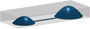
An approach capable of sidestepping the barriers of traditional microfluidic devices has recently been developed by Walsh et al. (Reference Walsh, Feuerborn, Wheeler, Tan, Durham, Foster and Cook2017). A partially wetting liquid (e.g. a liquid that will spread on a surface until an equilibrium thickness is reached) is printed on an unpatterned planar substrate and covered with an immiscible fluid to prevent evaporation. The footprint of such devices remains fixed when the contact angle is maintained between the advancing and receding values. This hysteresis can be large for several biologically relevant fluids. A variety of different experimental designs of these free surface microdevices have been developed, with varying degrees of complexity, some of which are illustrated in figure 1(a–c) (from Walsh et al. Reference Walsh, Feuerborn, Wheeler, Tan, Durham, Foster and Cook2017). In figure 1(a) a stable concentration is maintained across two laminar streams and in figure 1(b) different chemical dilutions are created in the four middle drops. Both of these devices can be used to study the behaviour of cells in different chemical environments, although the relation between device geometry and flow characteristics is complex. In contrast with conventional microfluidic devices, where fluid is pumped through solid conduits with a fixed geometry, in free surface microdevices both the shape of the conduits and the flow through them depend on the complex interplay between surface tension, buoyancy and viscosity. Hence, it is difficult to know a priori how to design a device with the most favourable characteristics.

Figure 1. (a–c) Images from experiments conducted by Walsh et al. (Reference Walsh, Feuerborn, Wheeler, Tan, Durham, Foster and Cook2017) showing some of the possible networks of drops and conduits. (d,e) The geometry and length scales of the simple dumbbell shaped circuit. The height of the conduit has been exaggerated for clarity; it is barely visible in (c). (f) The composite solution as described in § 3.7. Panels (a,c) are previously unpublished while (b) has been reproduced with permission from Walsh et al. (Reference Walsh, Feuerborn, Wheeler, Tan, Durham, Foster and Cook2017) with labels removed, under the creative commons licence, http://creativecommons.org/licenses/by/4.0/.
Further complications arise in analysing the experimental system of Walsh et al. (Reference Walsh, Feuerborn, Wheeler, Tan, Durham, Foster and Cook2017), due to their use of biological fluids and the associated surface adsorption of biological macromolecules, which are known to alter interfacial properties between two immiscible liquids (Carvajal et al. Reference Carvajal, Laprade, Henderson and Shull2011). However, even free surface devices constructed from liquids with constant surface tension present a challenging modelling problem in their own right and constitute a first step towards understanding free surface devices with more complicated interfacial phenomena.
Free surface fluid–fluid microdevices can be constructed with modular geometries, as highlighted by figure 1(b), necessitating a detailed consideration of how the basic building blocks, namely conduits and drops, interact in a microfluidic network. A thorough understanding of the flow through the simplest circuit, consisting of two drops connected by a single conduit so that the contact set has a ‘dumbbell’ shape (figure 1c), is required before progressing to more complicated networks.
A useful simplification in the limit of surface tension dominating gravity is that a sessile drop of fluid will take on the shape of a spherical cap and simple expressions can be found for the contact angle and radius of curvature. Using this approximation, Walsh et al. (Reference Walsh, Feuerborn, Wheeler, Tan, Durham, Foster and Cook2017) estimated the pressure at the base of the drop to be the Laplace pressure with a hydrostatic correction. Then assuming that the pressure at the base of the drop and in the conduit (near the inlet) are equal, the contact angle in the conduit can be estimated when there is no flow. To address more specific design questions, however, requires a more complete analysis of the dynamics of free surface devices. We anticipate that the large disparity in length scales between the different regions is likely to make numerical solution of the full free boundary problem computationally expensive. The disparity of length scales is, however, to the advantage of an asymptotic analysis. Thus the aim of this paper is to derive an asymptotic model for the long-term behaviour of viscous fluids in a constant surface tension, free surface microdevice using the standard thin-film equations (see e.g. Oron, Davis & Bankoff Reference Oron, Davis and Bankoff1997) and to analyse the fundamental fluid dynamics of networks, such as that of figure 1(b).
In § 2 we begin with a concise formulation of the lubrication equations governing the flow in a dumbbell configuration. In § 3 we will determine the asymptotic structure of the dumbbell problem in the distinguished limit in which the flow is driven by the pressure difference between drops. This will show that there are three distinct regions we need to consider and we identify the relevant time scales in each and the time scale over which the free surface of the whole device relaxes. It is the last of these time scales which will be most relevant for determining the duration of an experiment. On this time scale we find solutions of the lubrication equations in each region and form a composite solution for the thickness of the liquid over the whole domain. Quality control will be done via comparison of our asymptotic predictions with numerical simulations. We will then be able to illustrate qualitative trends in §§ 3.8 and 3.9. In § 4 the basic components of the simple dumbbell setup will then allow us to generalise to more complex networks. The implications of the current work and possible directions for future development are considered in § 5.
2. Formulation
2.1. Geometry for a dumbbell shaped circuit
The simplicity of the new devices means that complex circuits can be easily and quickly made by printing multiple drops and conduits. The simplest passive experimental set-up is the dumbbell shape contact set shown in figure 1(c). The circuit consists of a conduit with a rectangular base of width  $2a$ and length
  $L$, with fluid drops of base radii
  $R_L=\alpha _L L$ and
  $R_R=\alpha _R L$ at either end, the subscripts
  $_L$ and
  $_R$ corresponding to the left- and right-hand drops respectively. The circuit is then overlaid with an immiscible fluid of height
  $H$ above the substrate. We assume that the centres of the two drops are such that the length
  $L$ is the distance along the straight outer edge of the conduit as shown in figure 1(e). The initial volumes deposited in each drop and their base radii can be chosen so that there is a difference in pressure between the two drops. This pressure difference then drives the fluid along the conduit until the drop pressures are equalised. We let
  $H_D$ denote the height scale of a drop and
  $H_C$ the height scale of the conduit as shown in figure 1(d), and note that in practice
  $H_C \ll H_D \ll H$.
2.2. Lubrication equations
Throughout we shall assume that the fluid contained within the contact line forms a thin layer so that  $\delta = H_D /L \ll 1$. We introduce the Cartesian coordinates
  $({x^*},{y^*},{z^*})$ and time
  $t^*$, where the asterisks denote variables that are dimensional. The rigid, impermeable substrate is on the plane
  ${z^*}=0$ and
  ${x^*}$ is the distance along the conduit from the intersection with the left drop as shown in figure 1(e). The location of the free surface of the fluid is denoted by
  ${z^*}= {h^*}({x^*},{y^*},{t^*})$ with the film thickness
  $h^*$ assumed to be single-valued and positive on the interior of the contact set
  $\Omega ^*$. The large advancing and small receding contact angles ensure that for most cases the contact line
  $\partial \Omega ^*$ is pinned. The components of velocity in the
  ${x^*}$-,
  ${y^*}$- and
  ${z^*}$-directions are denoted by
  ${u^*}({x^*},{y^*},{z^*},{t^*})$,
  ${v^*}({x^*},{y^*},{z^*},{t^*})$ and
  ${w^*}({x^*},{y^*},{z^*},{t^*})$ and we let
  ${p^*}({x^*},{y^*},{z^*},{t^*})$ denote the corresponding pressure. The liquid in the dumbbell is assumed to be incompressible with constant density
  $\rho _1$ and to be governed at leading order (for small
  $\delta$) by the lubrication equations with a constant viscosity
  $\mu _1$, i.e.
 \begin{align} \frac{ \partial^{} {{p^*}} }{ \partial {{x^*}}^{} }=\mu_1 \frac{ \partial^{2} {{u^*}} }{ \partial {{z^*}}^{2} }, \quad \frac{ \partial^{} {{p^*}} }{ \partial {{y^*}}^{} }=\mu_1 \frac{ \partial^{2} {{v^*}} }{ \partial {{z^*}}^{2} }, \quad \frac{ \partial^{} {{p^*}} }{ \partial {{z^*}}^{} } = -\rho_1 g , \quad \frac{ \partial^{} {{u^*}} }{ \partial {{x^*}}^{} } + \frac{ \partial^{} {{v^*}} }{ \partial {{y^*}}^{} } + \frac{ \partial^{} {{w^*}} }{ \partial {{z^*}}^{} } =0, \end{align}
for  $0<{z^*}<{h^*}({x^*},{y^*},{t^*})$ and
  $({x^*}, {y^*}) \in \Omega ^*$, where
  $g$ is the acceleration due to gravity. There is no slip on, nor flux through, the substrate, so
 \begin{equation} {u^*}=0,\quad {v^*}=0,\quad {w^*}=0 \quad \text{on } {z^*}=0 \text{ for } ({x^*}, {y^*}) \in \Omega^*. \end{equation}
The appropriate boundary condition on the interface  $h^*$ depends on the overlaying liquid. We assume that the overlaying liquid is incompressible with constant density
  $\rho _2$ and governed by the Navier–Stokes equations with a constant viscosity
  $\mu _2$. The jump in pressure across the free surface is assumed to be due to a constant surface tension
  $\gamma$. If we further assume that the depth of the overlaying liquid
  $H$ is much larger than the height scale of the circuit
  $H_D$ and that the viscosity ratio
  $\mu = \mu _2 / \mu _1$ is order unity, we find that, at leading order, the only effect of the upper liquid layer is via the hydrostatic pressure in the normal stress boundary condition. That is to say, the shear stress exerted by the upper liquid is of a higher order than that generated by the flow in the circuit. Thus, at leading order, the pressure in the overlaying liquid is given by
  $P^* = \rho _2 g (H- z^*) +p_{{atm}}$, where
  $p_{{atm}}$ is atmospheric pressure, and the boundary conditions on the fluid interface are given by
 \begin{align} \frac{ \partial^{} {{u^*}} }{ \partial {{z^*}}^{} }=0, \quad \frac{ \partial^{} {{v^*}} }{ \partial {{z^*}}^{} }=0, \quad {w^*} = \frac{ \partial^{} {{h^*}} }{ \partial {{t^*}}^{} }+ {u^*}\frac{ \partial^{} {{h^*}} }{ \partial {{x^*}}^{} } + {v^*} \frac{ \partial^{} {{h^*}} }{ \partial {{y^*}}^{} }, \quad {p^*} = P^* - \gamma \nabla^2 {h^*} \end{align}
on  ${z^*}={h^*}({x^*},{y^*},{t^*})$ for
  $({x^*}, {y^*}) \in \Omega ^*$. Combining (2.1c) with (2.3d) then shows that the pressure in the underlying fluid satisfies
 \begin{equation} {p^*} = p_{{atm}} +\rho_2 g H - \gamma \nabla^2 {h^*} - {\rm \Delta} \rho g {h^*} - \rho_1g {z^*}, \end{equation}
where  ${\rm \Delta} \rho = \rho _2-\rho _1$. The velocity components are then found from (2.1), (2.2) and (2.3):
 \begin{equation} {u^*} = \frac{1}{2 \mu_1}\left( {{z^*}}^2 - 2 {h^*} {z^*} \right) \frac{ \partial^{} {{p^*}} }{ \partial {{x^*}}^{} }, \quad {v^*} = \frac{1}{2\mu_1}\left( {{z^*}}^2 - 2 {h^*} {z^*} \right) \frac{ \partial^{} {{p^*}} }{ \partial {{y^*}}^{} } . \end{equation}
Finally (2.1d), (2.2c) and (2.2c) give
 \begin{equation} \frac{ \partial^{} {{h^*}} }{ \partial {{t^*}}^{} } = \boldsymbol{\nabla} \boldsymbol{\cdot} \left(\frac{{h^*}^3}{3 \mu_1 } \boldsymbol{\nabla} {p^*} \right)\quad \text{for } ({x^*},{y^*}) \in \Omega^*, \end{equation}
where  $\boldsymbol {\nabla } = (\partial / \partial x^*,\ \partial / \partial y^* )$ is the two-dimensional gradient operator. Thus the equation we have to solve for the interface height is given by
 \begin{equation} \frac{ \partial^{} {{h^*}} }{ \partial {{t^*}}^{} } + \boldsymbol{\nabla} \boldsymbol{\cdot} \left(\frac{1}{3 \mu_1} {{h^*}}^3 \boldsymbol{\nabla}\left(\gamma \nabla^2 {h^*} + {\rm \Delta} \rho g {h^*} \right)\right)=0 \quad \text{for } ({x^*},{y^*}) \in \Omega^*, \end{equation}
with zero height on the contact line, no flux through the contact line and subject to a suitable initial condition.
2.3. Non-dimensionalisation and boundary conditions
We suppose that the drops may be large enough that we must account for the effects of gravity, but not so large that gravity dominates the effects of surface tension. We then use the drop height and conduit length to non-dimensionalise the vertical and horizontal components, respectively. We anticipate that different physical effects will be dominant at different time scales, but we initially use the time scale of capillary action in the drops, obtained by balancing the terms in (2.7). Thus, we non-dimensionalise by scaling
 \begin{gather} {x^*} = L x,\quad {y^*} = L y, \quad {z^*}=H_D z, \quad {t^*}=\frac{3 \mu_1 L}{ \delta^3 \gamma } {t}, \end{gather}
 \begin{gather}\boldsymbol{u}^* = \frac{\delta \gamma}{\mu_1}\left( u, v,\delta w \right)\!,\quad {h^*} =H_D h , \quad {p^*} = \frac{\gamma}{\delta L} p +p_{{atm}} + \rho_2 gH - \rho_1 g H_D z . \end{gather}
The definitions of physical parameters and the typical values that have been used in experiments are summarised in the upper section of table 1. The governing equation for the interface height (2.7) is then given by
 \begin{equation} \frac{ \partial^{} {h} }{ \partial {{t}}^{} } = \boldsymbol{\nabla} \boldsymbol{\cdot} \left( h^3 \boldsymbol{\nabla} p \right), \quad p=-\nabla^2 h - {Bo}\,h \quad \text{for } (x,y) \in \Omega, \end{equation}
where the Bond number is defined as  ${Bo} = (\rho _2 -\rho _1 )g L^2 / \gamma$ and
  $\Omega$ denotes the rescaled contact set bounded by the pinned contact line
  $\partial \Omega$. The Bond number has been defined so that it is positive when the overlaying liquid has higher density than the liquid in the circuit, as is typical in experiments (see table 1), although our model will still be valid for negative Bond numbers. The interface height is zero on the contact line and there is no flux through the contact line, so we impose the boundary conditions
 \begin{equation} h = 0, \quad h^3 \frac{ \partial^{} {p} }{ \partial {n}^{} } =0 \quad \text{for }(x,y) \in \partial \Omega, \end{equation}
where  $\partial / \partial n$ now denotes the outward normal derivative on
  $\partial \Omega$. Finally an initial condition
  $\mathcal {H}(x,y)$ needs to be prescribed for the interface height at time
  $t=0$, i.e.
 \begin{equation} h(x,y,0) = \mathcal{H}(x,y) \quad \text{for } (x,y) \in \Omega , \end{equation}
The leading-order model (2.8)–(2.12) is applicable for small  $\delta = H_D/L$, which we recall to be the ratio of the drop height scale and conduit length scale, and depends on four dimensionless parameters: the Bond number
  $Bo$, which gives a measure of the importance of gravitational forces compared to surface tension; the dimensionless radii of the bases of the two drops
  $\alpha _L$ and
  $\alpha _R$, as shown in figure 2; and, finally the aspect ratio of the conduit
  $\epsilon = a/L$, which gives a ratio of the conduit width to length. The typical values of the dimensionless parameters are shown in the lower half of table 1. We shall consider in § 3 the most physically relevant distinguished limit in which
  $Bo,\alpha _L,\alpha _R = {O}(1)$ as
  $\epsilon \to 0$.

Figure 2. The dimensionless contact set with each of the domains labelled:  $\Omega _{L}$ and
  $\Omega _{R}$ are the bases of the drops;
  $\Omega _C$ is the rectangular conduit, with a length of
  $1$ along its outer edge and a width of
  $2 \epsilon$;
  $\Omega _{JL}$ and
  $\Omega _{JR}$ are the junction regions where the drops intersect the conduit and
  $\partial \Omega$ is the pinned contact line.
Table 1. The physical parameters for water (the typical fluid that forms devices) and FC40 (the typical overlaying fluid) at room temperature and pressure, the typical range of geometric parameters used and the dimensionless parameters. All dimensional values are from Walsh et al. (Reference Walsh, Feuerborn, Wheeler, Tan, Durham, Foster and Cook2017).

2.4. Global mass conservation
One of our main aims will be to predict the time scale over which the volumes of the two drops equilibrate; i.e. the time scale of drop drainage. We divide the contact set  $\Omega$ into three regions: the conduit region is defined by
  $\Omega _C=\{ (x,y) : 0 < x < 1,\ |y| <\epsilon \}$, then the left-hand drop region is bounded by a circular arc of radius
  $\alpha _L$ which intersects the conduit at
  $(x,y) = (0,\pm \epsilon )$, while the right-hand drop region is similarly defined as shown in figure 2. We define the volumes in the left drop, conduit and right drop to be given by
 \begin{equation} {V_L}({t}) = \iint_{\Omega_L} {h} \,\text{d} {x} \,\text{d} {y} ,\quad {V_C}({t}) = \iint_{\Omega_C} {h} \,\text{d} {x} \,\text{d} {y} ,\quad {V_R}({t}) = \iint_{\Omega_R} {h} \,\text{d} {x} \,\text{d} {y}. \end{equation}
Since there is no flux of liquid through the pinned contact line, the total volume in the device is given by the initial volume,  $V$, as follows
 \begin{equation} {V_L} +{V_C}+{V_R} = \iint_{\Omega} \mathcal{H}(x,y)\,\,\text{d} {x}\,\text{d} {y} ={V}. \end{equation}
The dimensionless area of, and flux through, a cross-section of the conduit in an  $x$-plane (with
  $0<x<1$) are given at leading order by
 \begin{equation} {A}({x},{t}) = \int_{-\epsilon}^{\epsilon} {h}\,\,\text{d} {y},\quad {Q}({x},{t}) =\int_{-\epsilon}^{\epsilon} \int_0^{h} {u}\,\,\text{d} {z}\,\text{d} {y} = -\int_{-\epsilon}^{\epsilon} {h}^3 \frac{ \partial^{} {{p}} }{ \partial {{x}}^{} } \,\text{d} {y} . \end{equation}
Integrating (2.8) over the conduit cross-section then gives
 \begin{equation} \frac{ \partial^{} {{A}} }{ \partial {{t}}^{} } + \frac{ \partial^{} {{Q}} }{ \partial {{x}}^{} }=0\quad \text{for } 0<{x}<1. \end{equation}
Alternatively, integrating (2.8) over the three regions  $\Omega _L$,
  $\Omega _C$ and
  $\Omega _R$ shows that the volume of liquid in each region evolves according to the ordinary differential equations given by
 \begin{equation} \frac{ \text{d}^{} {{V_L}} }{ \text{d} {{t}}^{} } = -{Q_L}({t}),\quad \frac{ \text{d}^{} {{V_R}} }{ \text{d} {{t}}^{} } = {Q_R}({t}),\quad \frac{ \text{d}^{} {{V_C}} }{ \text{d} {{t}}^{} } = {Q_L}({t})-{Q_R}({t}), \end{equation}
where we have defined  $Q_L(t) = Q(0,t)$ and
  $Q_R(t) = Q(1,t)$ to be the fluxes where the conduit connects to the left and right drop respectively. The expressions (2.16) and (2.17) will play a key role in our scaling and subsequent asymptotic analysis, in which they will be used to close the leading-order governing equations (rather than proceeding to higher order).
3. Asymptotic analysis for a long, thin conduit
3.1. Asymptotic structure and time scales
The two main aims of the dumbbell set-up are (i) for the pressure difference between the two drops to be the dominant mechanism that drives fluid through the conduit; and (ii) for the flux through the conduit to vary slowly over time. To achieve aim (i) we require the pressure in the drops and conduit to be comparable, where the dimensionless pressure in a drop is  ${O}(1)$. In the conduit we scale
  $y \sim \epsilon$, then balancing the pressure with the first term on the right-hand side of (2.10b) shows that we must print liquid of thickness
  $h \sim \epsilon ^2$ in the conduit in order for the pressures to balance. To achieve aim (ii) we require the conduit to be long and narrow i.e.
  $\epsilon \ll 1$. We will show that the resulting asymptotic structure consists of five regions: two drops with contact sets
  $\Omega _L$ and
  $\Omega _R$, a narrow and thin conduit with contact set
  $\Omega _C$, and two small junction regions with contact sets
  $\Omega _{JL}$ and
  $\Omega _{JR}$ connecting together the drops and conduit, as illustrated in figure 2.
Given our assumptions about the geometry of the device we can now describe the different physical time scales and show that drainage (the time scale on which the pressure equilibrates) acts on a much longer time scale than anything else in the model. In the three regions we have defined we can use a dominant balance argument in (2.8) to find the time scale of capillary action in each region. In the conduit region we scale with  $y \sim \epsilon$ and
  $h \sim \epsilon ^2$; in the junction region we scale with
  $x,y,h \sim \epsilon$. These scalings and (2.8) give us the dimensionless time scales of capillary action in the junction and conduit, respectively, as
  $t_J\sim \epsilon$ and
  $t_{CW}\sim \epsilon ^{-2}$. Since we assume that the conduit is much longer than it is wide
  $t_{CW}$ is the time scale of relaxation (of the free boundary) across the width of the conduit. The time scale of relaxation of the free boundary along the length of the conduit is found by balancing the terms in (2.16). The cross-sectional area and flux in the conduit in (2.15) are also rescaled with
  $y \sim \epsilon$ and
  $h \sim \epsilon ^2$, so that
  $A \sim \epsilon ^3$ and
  $Q \sim \epsilon ^7$; hence, the time scale for relaxation along the length of the conduit is
  $t_{CL} \sim \epsilon ^{-4}$. The drainage time scale is then found by balancing the terms in (2.17). With the same length scales as above for the flux, we still have
  $Q \sim \epsilon ^7$, but the relevant length scale for the volume gives
  $V_L ={O}(1)$ (since all the fluid is contained in the drop regions at leading order). Thus the time scale for drop drainage is
  $t_{DD} \sim \epsilon ^{-7}$.
We have identified five time scales thus far, each depending on the conduit aspect ratio  $\epsilon$. They are, respectively, the relaxation time scales for the junction, drops, conduit width and conduit length and the drainage time scale
 \begin{equation} t_{J} \sim \epsilon, \quad t_{D} \sim 1, \quad t_{CW}\sim \frac{1}{\epsilon^2}, \quad t_{CL} \sim \frac{1}{\epsilon^4} , \quad t_{DD}\sim \frac{1}{\epsilon^7}. \end{equation}
To achieve slowly varying fluxes and stresses we need  $t_{DD}$ to be much larger than
  $t_{CL}$, and we can also already see that the drainage time scale is very sensitive to
  $\epsilon$, so that the geometry is an important factor in achieving a given flux.
3.2. Quasi-steady solution in the drops
The leading-order analysis is the same in each drop, so we give only the details for the left-hand one. The conduit is in the much smaller junction region, so at leading order the relevant contact set in the drop is the circular disc  $\Omega _{L0}$ of radius
  $\alpha _L$ with centre
  $(x,y) = (-\alpha _L,0)$. For
  $t \gg t_{D} \sim 1$, the profile is quasi-steady, with spatially uniform pressure at leading order. The boundary condition (2.11a) holds at leading order on the boundary of the contact set except at the origin (i.e. on
  $\partial \Omega _{L0} / \{(0,0)\}$); at the origin we must instead match with the junction region. Since the height scale in the junction region is of
  ${O}(\epsilon )$, the relevant matching condition is that the leading-order film thickness tends to zero as
  $(x,y) \to (0,0)$, with
  $(x,y) \in \Omega _{L0}$. Hence, at leading order, the drop profile is as if there was no junction region and therefore axisymmetric.
We introduce the polar coordinate  $r=\sqrt {(x+\alpha _L)^2 +y^2}$ measuring radial distance from the centre of the circular contact set of the left-hand drop. Then, expanding
  $h \sim h_L(r,t)$ and
  $p\sim p_L(t)$ as
  $\epsilon \to 0$, we deduce from (2.8)–(2.9) the familiar leading-order governing equations given by
 \begin{equation} \frac{ \partial^{2} {h_L} }{ \partial {r}^{2} } +\frac{1}{r} \frac{ \partial^{} {h_L} }{ \partial {r}^{} } +Bo\, h_L = -p_L \quad \text{for } 0 < r < \alpha_L, \end{equation}
with  $|h_L(0,t)| < \infty$ and
  $h_L(\alpha _L ,t)=0$; the pressure is related to the leading-order drop volume by the conservation of mass constraint that
 \begin{equation} 2 {\rm \pi}\int_0^{\alpha_L} r h_L\,\text{d} r = V_L(t), \end{equation}
where  $V_L(t)$ now denotes the leading-order volume in the left-hand drop (for small
  $\epsilon$). Thus the leading-order problem in the left-hand drop has been reduced to the classical one of finding the shape of a static liquid drop with constant surface tension and gravity, which has been well studied with well-known interface shape when the contact angle is small (see, for instance, Chesters Reference Chesters1977; Thomson Reference Thomson1886). Subject to the additional constraint that we require the drop thickness and pressure to be positive away from the contact line (as discussed below), the solution for
  $Bo\ne 0$ is given by
 \begin{equation} h_L=\left( \frac{ J_{0}\left(\sqrt{Bo}\, r \right) }{ J_{0}\left(\sqrt{Bo} \,\alpha_L \right) } -1 \right) \frac{p_L}{Bo}, \quad h_R=\left( \frac{ J_{0}\left(\sqrt{Bo}\, r\right)}{ J_{0}\left(\sqrt{Bo} \,\alpha_R\right)} -1 \right) \frac{p_R}{Bo}, \end{equation}
where  $J_n$ is the Bessel function of the first kind of order
  $n$ and the pressures are a linear function of the volume given by
  $p_L = \beta _L V_L$ and
  $p_R = \beta _RV_R$ (where
  $V_R(t)$ now denotes the leading-order volume in the right-hand drop for small
  $\epsilon$). The constants relating the pressure to the volume in the left- and right-hand drops are defined as
 \begin{equation} \beta_{L} = \frac{ Bo \, J_{0}\left(\sqrt{Bo} \, \alpha_L \right)}{{\rm \pi} \alpha_{L}^2 J_{2}\left(\sqrt{Bo} \, \alpha_L\right)} , \quad \beta_{R} = \frac{ Bo \, J_{0}\left(\sqrt{Bo} \, \alpha_R \right)}{{\rm \pi} \alpha_{R}^2 J_{2}\left(\sqrt{Bo} \, \alpha_R\right)} . \end{equation}
Since the square root of the Bond number appears in the argument of the Bessel functions in (3.4)–(3.5), they have an imaginary argument when the liquid in the circuit is denser than the overlaying liquid (i.e.  $Bo < 0$). In this case the solution may written in terms of modified Bessel functions; these give a profile which decreases monotonically from the origin, whereas the original Bessel functions are oscillatory. We do not allow for solutions with either negative drop thicknesses or negative pressure anywhere;
  $h_L$,
  $h_R$,
  $p_L$ and
  $p_R$ are everywhere positive if and only if
  $\alpha _L \sqrt {Bo} < \lambda$ and
  $\alpha _R \sqrt {Bo} < \lambda$, where
  $\lambda \approx 2.405$ is the smallest positive root of
  $J_0$. There is therefore a critical Bond number
  $Bo_C = min(\lambda ^2 /\alpha _R, \lambda ^2 /\alpha _R)$ beyond which at least one of the leading-order quasi-steady solutions above would cease to exist. However, we must also ensure that the contact line remains pinned, i.e. that the contact angle remains between the receding and advancing values. This constraint is even more restrictive than the one on the Bond number, and best addressed once we have derived the corresponding leading-order solutions in the conduit and junction region, so we defer a discussion until later on (see § 3.8).
3.3. Quasi-steady solution in the conduit
The footprint of the conduit is a rectangle of width  $2\epsilon$ and length
  $1$. On the long edges of the conduit the interface will have zero height where the contact line is pinned. The appropriate boundary condition at the ends will be derived below by matching with the junction regions. As with the solution in the drops we note that the problem of flow in a fluid rivulet has also been well studied (see, for instance, Towell & Rothfeld Reference Towell and Rothfeld1966; Paterson, Wilson & Duffy Reference Paterson, Wilson and Duffy2013). Earlier we deduced that we need
  $h\sim \epsilon ^2$ in order for the pressure difference between the drops to be the dominant mechanism driving the flow. Thus we rescale the governing equations with
 \begin{equation} {y} = \epsilon \hat{y}, \quad h= \epsilon^2 \hat{h}_C. \end{equation}
Provided  $t \gg t_{CW}\sim \epsilon ^{-2}$, the pressure is then spatially uniform in each
  ${x}$-plane at leading order. Expanding
  $\hat {h}\sim \hat {h}_C(x,\hat {y},t)$ and
  $p\sim p_C(x,t)$ as
  $\epsilon \to 0$ in (2.10b) then gives
 \begin{equation} \frac{ \partial^{2} {\hat{h}_C} }{ \partial {\hat{y}}^{2} }=- p_C \quad \text{for }-1 < \hat{y}<1. \end{equation}
Since  $\hat {h}_C = 0$ at
  $\hat {y} = \pm 1$ for
  $0 < x < 1$, we deduce that the interface height has a parabolic profile in each cross-section given by
 \begin{equation} \hat{h}_C = \frac{p_C}{2} \left( 1-\hat{y}^2 \right) . \end{equation}
It follows from (2.15) that the corresponding leading-order expressions for the area and flux in the conduit are given by
 \begin{equation} A \sim \frac{2}{3}\epsilon^3 p_C, \quad Q \sim -\frac{1}{35} \epsilon^7 \frac{ \partial^{} {} }{ \partial {{x}}^{} }\left( p_C^4 \right) \quad \text{as } \epsilon \to 0. \end{equation}
3.4. Quasi-steady solution in the junction regions
The junction regions, which connect the conduit to the drops, are indicated by the boxes in figure 2. Without loss of generality we will consider only the junction connecting the conduit to the left drop. Since the film thickness is of  ${O}(1)$ in the drops the pertinent scalings in the left-hand junction region are given by
 \begin{equation} x = \epsilon \tilde{x}, \quad y = \epsilon \tilde{y}, \quad h=\epsilon \tilde{h}. \end{equation}
The contact line of the left-hand drop then satisfies
 \begin{equation} \left(\epsilon \tilde{x} +\sqrt{\alpha_L^2-\epsilon^2} \right)^2+ \epsilon^2 \tilde{y}^2 = \alpha_L^2 \quad \text{for } \tilde{x} \leq0, \end{equation}
so that it lies at  $\tilde {x} =0$ for
  $| \tilde {y}| \geq 1$ at leading order as
  $\epsilon \to 0$ with
  $\tilde {y} = {O}(1)$. The leading-order geometry of the contact set in the junction region is therefore as illustrated in figure 3: the contact set of the drop fills the left half-plane
  $\tilde {x} < 0$, while that of the conduit fills the semi-infinite strip
  $|\tilde {y}|<1$,
  $\tilde {x}\geq 0$. The interface height in the junction region is governed by (2.8), with the solution needing to match with the conduit solution (3.8) as
  $\tilde {x} \to \infty$ and with the drop solution (3.4) as
  $\tilde {x}^2+\tilde {y}^2 \to \infty$ in the left half-plane, with (2.9) still holding on the contact lines at
  $\tilde {x}=0$,
  $\tilde {y} \geq 1$. For
  $t \gg t_J \sim \epsilon$, the evolution is again quasi-steady with spatially uniform pressure at leading order. However, the disparity in the film thicknesses in the drop, junction and conduit regions (where
  $h$ is of
  ${O}(1)$, of
  ${O}(\epsilon )$ and of
  ${O}(\epsilon ^2)$, respectively) means that we must now proceed to second order in the analysis in order to span these length scales: expanding
  $h \sim \tilde {h}_0(\tilde {x}, \tilde {y},t) + \epsilon \tilde {h}_1(\tilde {x},\tilde {y},t)$ and
  $p \sim p_{JL}(t)$ as
  $\epsilon \to 0$, we find that
  $\tilde {h}_0$ and
  $\tilde {h}_1$ satisfy the leading- and second-order problems summarised in figure 3 in which we have also recorded the boundary conditions on the contact line and the far-field conditions that must be imposed in order to match with the adjoining drop and conduit. The mean curvature of the leading-order film thickness is equal to zero because the leading-order pressure appears first in the second-order problem for the correction to the film thickness. We note that if the leading-order pressure were an order of magnitude larger then it would not be possible to match it with the pressures in the adjoining drop and conduit (as detailed below); nor would it be possible to match the leading-order film thickness with that in the drop (because this requires the leading-order film profile to be linear in the far field). At leading order the height is zero on the contact line (given by (2.9)) and also tends to zero in the conduit as
  $\tilde {x} \to \infty$ since the interface height is
  ${O}(\epsilon )$ there. Expanding the solution in the drop (3.4) as
  $r\to \alpha _L^{-}$ gives the leading-order far-field condition as
  $\tilde {x}^2+ \tilde {y}^2 \to \infty$, where the leading-order contact angle
  $\theta _L$ is given by
 \begin{equation} \theta_L = \frac{J_{1}\left(\sqrt{Bo} \, \alpha_L \right)}{\sqrt{Bo}\, J_{0}\left(\sqrt{Bo} \, \alpha_L \right)} p_L. \end{equation}
At second order the interface height is still zero on the contact line in the conduit, but on  $\tilde {x}=0$ we have to take account of the curvature of the contact line. In the conduit the far-field condition comes from matching with the conduit solution (3.8). To find the leading-order far-field condition in the drop we expanded (3.4) as
  $r \to \alpha _L^{-}$: the next term in this expansion gives the far-field condition at second order.

Figure 3. (a) The leading-order problem in the junction region. (b) The second-order problem in the junction region, where  $\tilde {h}_{\infty } = \theta _L(\tilde {x}^2 - \tilde {y}^2 )/(2 \alpha _L ) - p_L \tilde {x}^2 / 2$. The junction region is defined as
  $\Omega _J =\{ (\tilde {x},\tilde {y}): \tilde {x} <0 \} \cup \{(\tilde {x},\tilde {y}) : |\tilde {y} | <1,\ \tilde {x} \geq 0 \}$, see text for details.
The boundary value problems in figure 3 may be solved using standard conformal mapping techniques (see, e.g. Driscoll & Trefethen Reference Driscoll and Trefethen2002). We find the leading-order solution to be given implicitly by
 \begin{equation} \tilde{h}_0 =\frac{2 \theta_L }{{\rm \pi} }\textrm{Re} \left(f^{-1}(\tilde{z})\right), \end{equation}
where  $\tilde {z}=\tilde {x}+\textrm {i}\tilde {y}$ and the transform
  $\tilde {z} = f(\zeta )$ maps the lower half
  $\zeta$-plane to the junction region in the
  $\tilde {z}$-plane and is given by
 \begin{equation} f\left( \zeta \right) = \frac{2 \,\textrm{i} }{\rm \pi} \left( \sqrt{\zeta^2-1} + \sin^{-1}\left( \frac{1}{\zeta}\right) \right), \end{equation}
where  $\zeta = \xi + \textrm {i} \eta$. At
  ${O}(\epsilon )$ the governing equation for the interface height is
  $\nabla ^2\tilde {h}_1 = -p_{JL}(t)$ in
  $\Omega _J$. Substituting the conduit far-field condition therefore gives
  $p_{JL}(t) = p_C(0,t)$; similarly substituting the drop far-field condition gives
  $p_{JL}(t) = p_L(t)$; we deduce that the pressure passes straight through the junction at leading order, i.e.
 \begin{equation} p_{JL}(t) = p_L(t)=p_C(0,t). \end{equation}
To find the next order solution we first subtract from  $\tilde {h}_1$ the far-field solution in the drop as
  $\tilde {x}^2+\tilde {y}^2\to \infty$, so that we are again solving Laplace's equation in the junction region. This will allow us to use the same conformal mapping techniques as we did for the leading-order problem. The details are presented in appendix A. An example of the leading- and second-order solutions are shown in figure 4. As we approach the corner along the contact line the slope of both these solutions becomes infinite. This will have implications for the pinning of the contact line as we shall discuss in § 3.8.

Figure 4. Plots of the leading-order solution and the second-order correction in the junction region for  $Bo = 8$ and
  $\alpha _L = 0.5$. The location of the substrate is indicated by the grid with the conduit extending in the positive
  $\tilde {y}$-direction. (a) The leading-order solution given by (3.13). (b) The second-order solution given by (A 14).
3.5. Conduit relaxation
As detailed in § 3.1, the conduit relaxes on the time scale  $t_{CL} \sim \epsilon ^{-4}$; this was derived from (2.15). Using (2.15), (2.16) and making the rescaling
  $t = (70 /3)\epsilon ^{-4} \tau$, we derive an equation for the conduit pressure on the time scale of conduit relaxation
 \begin{equation} \frac{ \partial^{} {p_C} }{ \partial {{\tau}}^{} } = \frac{ \partial^{2} {} }{ \partial {x}^{2} }\left(p_C^4 \right)\quad \text{for } 0 < x < 1, \tau > 0. \end{equation}
In § 3.4 we deduced that the leading-order pressure in the junction regions is spatially uniform and equal to the pressure in the adjacent drop and conduit as long as  $t\gg t_{J} \sim \epsilon$. Since
  $t_{CL}\gg t_{J}$ as
  $\epsilon \to 0$, the pressure at the ends of the conduit will be equal to the pressure in the corresponding drop. Furthermore, since
  $t_{DD} \gg t_{CL}$ the leading-order pressure in the drops will not have changed, so the relevant boundary conditions for (3.16) are given by
 \begin{equation} p_C(0,\tau) = p_L(0),\quad p_C(1,\tau) = p_R(0) \quad \text{for }\tau >0, \end{equation}
where the pressures in the left- and right-hand drops,  $p_L$ and
  $p_R$, can be related to their respective volumes,
  $V_L$ and
  $V_R$, by (3.5)). The problem is closed by prescribing an initial condition of the form
 \begin{equation} p_C( x,0) = \mathcal{P}(x) \quad \text{for } 0 < x < 1. \end{equation}
For a positive and sufficiently regular initial profile we anticipate the long-time attractor to be the steady-state solution, so that
 \begin{equation} p_C \to \left( \left(p_R^4 -p_L^4 \right)x+p_L^4 \right)^{{1}/{4}} \quad \text{as }\tau \to \infty. \end{equation}
Examples of the solution of the time-dependent problem are shown in figures 5(a) and 5(b) (solid lines); they tend to (3.19) (dashed line) as  $\tau$ increases and the steady state is reached much faster when the initial pressure gradient is increased.

Figure 5. (a,b) Numerical solution of the conduit relaxation problem (3.16)–(3.18) for different boundary conditions (drop pressures), where the initial profile is linear. The dashed line is the steady-state solution given by (3.19). In (a)  $\tau = 0 , 0.0064, 0.0320$, whereas in (b)
  $\tau = 0 , 0.0005, 0.0020$. (c) The evolution of the left-hand drop volume given by (3.22) and (3.23) for
  $\mathcal {V}/V = 0.4,0.7 ,0.9$; in each case
  $\alpha = 0.25$ and (3.24) shows that the solutions tend to
  $0.8$.
3.6. Droplet drainage
On the time scale of drainage  $t_{DD} \sim \epsilon ^{-7}$, the pressure in the conduit is quasi-steady and therefore given by the right-hand side of the expressions in (3.19). We can then use (3.9b) to find that the flux in the conduit on this time scale is given by
 \begin{equation} Q \sim \epsilon^7 \frac{p_L^4-p_R^4}{35}. \end{equation}
When  $\epsilon \ll 1$ most of the fluid is contained in the drops, with the conduit containing very little fluid. We can therefore use (2.17) to find ordinary differential equations (ODEs) for the volume in each drop. Substituting (3.20) into (2.17a,b) gives
 \begin{equation} \frac{ \text{d}^{} {V_L} }{ \text{d} {t}^{} }\sim - \epsilon^7 \frac{p_L^4-p_R^4}{35},\quad \frac{ \text{d}^{} {V_R} }{ \text{d} {t}^{} }\sim \epsilon^7 \frac{p_L^4-p_R^4}{35}. \end{equation}
Since the drop pressure is a linear function of the volume (with the constants of proportionality given by (3.5)) we can write (3.21) entirely in terms of the drop volumes. At leading order the volume in the conduit scales with  $\epsilon ^3$ (as can be seen from (2.13b). Assuming that
  $V_L(0),V_R(0) \gg \epsilon ^3$, at leading order the total volume
  $V$ is given by the sum of the volumes of the two drops, which is a constant since no fluid is leaving the system. If we then rescale time with
  $t = 35/(V^3 \beta _R^4) \epsilon ^{-7}T$, we need only solve a single ODE given by
 \begin{equation} \frac{ \partial^{} {} }{ \partial {{T}}^{} } \left( \frac{V_L}{V} \right)= \left( 1-\frac{V_L}{V} \right)^4 -\alpha^4\left( \frac{V_L}{V} \right)^4, \end{equation}
where  $\alpha ^4 = \beta _L^4/ \beta _R^4$. To close this problem we will need an initial volume for the left drop of the form
 \begin{equation} {V}_L(0) = \mathcal{V}. \end{equation}
The powers of four in (3.22) suggest that there could be multiple steady-state solutions, but we find that only one of them is real and in the range  $[0,V]$, so the volume of the left drop can only tend to one value given by
 \begin{equation} \frac{{V}_L}{V} \to \frac{1}{1+\alpha} \quad \text{as } {{T}} \to \infty. \end{equation}
Equation (3.22) is separable which allows us to easily find an implicit solution, which in the case of  $\alpha = 1$ collapses to
 \begin{equation} \frac{{V}_L}{V} =\frac{1}{2} \left( 1 + \frac{ 1}{ \sqrt{A\,\textrm{e}^{ 2 T} - 1}}\right),\quad A = 1+ \frac{1}{\left( 2\mathcal{V} -1 \right)^2}. \end{equation}
Some examples of the evolution of the left-hand drop volume are plotted in figure 5(c) for different initial volumes.
3.7. Numerical validation
In this section we will describe our numerical simulations of the full thin-film boundary value problem given by (2.8)–(2.12) on the domain indicated in figure 1(e), and compare the results with the asymptotic predictions we have obtained. The numerical simulations are performed with COMSOL Multiphysics® via the thin-film flow toolbox, using COMSOL's ‘fine mesh’ option and in-built algorithms that suitably refine the mesh in narrow regions of the domain geometry (COMSOL Multiphysics®v.5.4 2018).
We specify the initial volumes of the two drops; with this we can form a piecewise approximation to the interface height and pressure using (3.4) in the drops and (3.8) and (3.19) in the conduit. There will be discontinuities at either end of the conduit so we initially run the simulation on the junction relaxation time scale  $t_J$ to smooth out the initial condition. We use this piecewise construction of the initial condition rather than a composite solution because it is easier to implement and the junction regions relax on a much faster time scale than those we are interested in. For intermediate values of
  $\epsilon$ (
 $\epsilon >0.5$) the numerical solution can be found in a matter of seconds, but as anticipated, for smaller values of
  $\epsilon$ we find run times can increase by multiple orders of magnitude. This underlines how our asymptotic approach can facilitate the rapid prototyping of microfluidic system designs.
In figure 6 we compare the solution of (3.22) with numerical solutions for various small values of  $\epsilon$. In each simulation only the width of the conduit was altered and the initial drop volumes were fixed. In figure 6(a) we see good agreement over a range of values of
  $\epsilon$ for the volumes of the left (upper dashed line) and right (lower dashed line) drops as a function of time. The drainage solution can also be used to find the shear stress in the conduit. In the
  $x$-direction the leading-order dimensionless shear stress on the substrate is given by
 \begin{equation} {s} = \frac{ \partial^{} {u} }{ \partial {z}^{} } \bigg|_{z=0} = -h \frac{ \partial^{} {p} }{ \partial {x}^{} } = \frac{\left( \epsilon^2 - y^2\right) \left( p_L^4-p_R^4 \right) }{8 \sqrt{p_L^4 -\left(p_L^4 - p_R^4 \right)x }}, \end{equation}
where the dimensional shear stress is  $s^* = \gamma s /L$. The maximum shear stress is on
  $y=0$ at either
  $x=0$ or
  $x=1$ depending on the direction of the flow; the maximum will be at the junction near the conduit outlet. In figure 6(b) we compare the absolute maximum of the shear stress found in Comsol with the asymptotic prediction in (3.26). Again, as
  $\epsilon$ is decreased we see good agreement. For the flux given by (3.20), we first rescale with
 \begin{equation} Q = \frac { V^4 \beta_R^4 } {\epsilon^7 35} {\mathcal{Q}}, \end{equation}
then we find larger relative errors as can be seen in figure 6(c), especially on shorter time scales. Nevertheless there is still good agreement as  $\epsilon$ is decreased. This is shown in figure 6(d), where the root mean squared error of the flux over a unit time interval on the drainage time scale can be seen to decrease linearly as
  $\epsilon$ is reduced by more than an order of magnitude. Furthermore, this behaviour is also consistent with the root mean squared flux error over a unit time converging linearly to zero as the asymptotically small parameter is reduced, evidencing the validity of both the asymptotics and the finite element simulations.

Figure 6. Comparison of Comsol solutions with model predictions for different values of the small parameter  $\epsilon$. In each case the calculations were performed using
  $\alpha _{L} = \alpha _{R} = 1$ and
  $Bo=2$ with the initial volumes
  ${V}_L(0) = 0.2$ and
  ${V}_L(0) = 0.1$. (a–c) The solid lines show the numerical solution for
  $\epsilon = 0.01,0.1,0.2$ and the dashed line shows the asymptotic approximation. We compare (a) the drop volumes, given by (3.22); (b) the maximum shear stress on the substrate given by (3.26) with
  $y=0$ and
  $x=1$; and (c) the flux given by (3.20) and (3.27). (d) The root mean squared error of the flux over a unit time interval for different values of
  $\epsilon$, where
  $\mathcal {Q}_N$ is the numerical solution.
We are now in a position to construct a piecewise additive composite solution for the film height over the whole contact set  $\Omega$. Since the solutions found in the drop and conduit regions are only valid in those regions we form a piecewise solution. In the left drop the composite solution is found by adding the junction solution to the drop solution and then subtracting the overlap; in this case the two leading terms in the limit
  $\tilde {x}^2+\tilde {y}^2 \to \infty$ as shown in figure 3. The solution in the right drop is found in a similar way. In the conduit,
  $0< x <1$, we must find the junction solutions at either end of the conduit and add them both to the conduit solution (given by (3.8) and (3.19)); the overlaps are then the conduit solutions at
  $x=0$ and at
  $x=1$, so these are both subtracted. An example of the composite solution for the interface is shown in figure 1(f); the dimensionless parameters used are
  $Bo = 20$,
  $\alpha _L = 0.5$,
  $\alpha _R = 0.4$,
  $\epsilon = 0.05$,
  $V_L = 0.03$ and
  $V_R = 0.03$; since the base radii of the drops are different the same volumes will give different pressures. In figure 7 we plot the composite interface height (dashed line) along the centre of the conduit, i.e. on
  $y=0$ for different values of
  $\epsilon$. The left and right panels show the profile in the respective drop regions and the central panels show the solution in the conduit region. The solid line shows the corresponding numerical solution; we see particularly good agreement in the drop regions as
  $\epsilon$ is decreased. In the conduit the composite solution is able to pick out the location of the dip in conduit height near the outlet (the flow is from left to right), although it predicts a less sharp decrease in profile height. This dip is where the maximum shear stress occurs in the numerical solution.

Figure 7. Comparison of Comsol solution with the composite solution described in § 3.7 on  $y=0$. The calculations were performed using
  $\alpha _{L} = \alpha _{R} = 1$ and
  $Bo=4$ with the initial volumes
  ${V}_L(0) = 0.1$ and
  ${V}_L(0) = 0.05$. The solid lines show the numerical solutions and the dashed lines the corresponding asymptotic approximation. We compare the solutions on the drainage time scale, i.e.
  $t \gg \epsilon ^{-4}$. From top to bottom we have
  $t \sim 2.4\times 10^8,\ 3.9\times 10^9,\ 1.5\times 10^{11}$. The solutions for the left- and right-hand drop regions are shown on the left- and right-hand sides respectively, the conduit region is shown in the middle panels; note that the height scales with
  $\epsilon ^2$ in the conduit.
3.8. Maintaining a pinned contact line
Important features of these devices are the large advancing and small receding contact angles,  $\theta _a$ and
  $\theta _r$ respectively, which allows the volume of fluid in a drop to change significantly without the contact line moving. The particular values are highly dependent on the materials and fluids used, although Walsh et al. (Reference Walsh, Feuerborn, Wheeler, Tan, Durham, Foster and Cook2017) observe values of
  $\theta _r \sim 0.05$ radians and
  $\theta _a \sim 1.2$ in their experiments (while Lee, Lee & Doyle (Reference Lee, Lee and Doyle2015) measure
  $\theta _r \sim 0.5$ and
  $\theta _a \sim 1.0$ for water in decane on hydrophilic surfaces). Using the leading-order solutions (3.4) and (3.8), the contact angles in the left- and right-hand drops and the conduit, denoted by
  $\theta _L(t)$,
  $\theta _R(t)$ and
  $\theta _C(x,t)$ respectively, are given by
 \begin{equation} \theta_L = \frac{J_{1}\left(\sqrt{Bo} \, \alpha_L \right)}{\sqrt{Bo}\, J_{0}\left(\sqrt{Bo} \, \alpha_L \right)} p_L,\quad \theta_R =\frac{J_{1}\left(\sqrt{Bo} \, \alpha_R \right)}{\sqrt{Bo}\, J_{0}\left(\sqrt{Bo} \, \alpha_R \right)} p_R,\quad \theta_C = \epsilon \, p_C. \end{equation}
Since we are in the thin-film limit ( $\delta \ll 1$) we will have
  $\theta _L,\theta _R,\theta _C < \theta _a$. The same, however, cannot be said of the contact angle in the junction regions; as we saw in § 3.4 the contact angle tends to
  ${\rm \pi} /2$ at the corners where the drop meets the conduit. In practice the contact line near this corner will move outwards until the contact angle falls to the advancing angle. We expect the smoothing of the corner to happen on a length scale of the width of the conduit and on a time scale not much larger than that of capillary action in the junction regions. On the time scale
  $t \gg t_{CL} \sim \epsilon ^{-4}$, the smallest contact angle in the conduit will occur at the outlet where
  $p_C=min(p_L, p_R)$. As we are focusing on the distinguished limit in which
  $Bo,\alpha _L,\alpha _R = {O}(1)$ as
  $\epsilon \to 0$ we deduce that the contact angle in the conduit is always less than in the drops, so that the leading-order contact angle is everywhere – subject to the caveat above concerning the corners – greater than or equal to the receding contact
  $\theta _r$ provided
 \begin{equation} \theta_{min} = \epsilon min \left( \beta_L V_L , \beta_R V_R \right) \geq \theta_r,\end{equation}
where we have used (3.4), (3.5) and (3.28c). We note that this constraint is satisfied for all  $t> 0$ only if it is satisfied initially, so that the contact line remains pinned only if it is pinned initially. We further note that in accordance with physical intuition it is easier to satisfy the constraint (3.29) the larger the volumes of the drops or the smaller the radii of their contact sets, but a complete characterisation is complicated due to the non-monotonic dependence of
  $\beta _L$ and
  $\beta _R$ on the Bond number
  $Bo$, although (3.29) is of course readily checked for specific parameter values. Henceforth we shall assume that
  $\theta _r$ may be engineered to be sufficiently small that the constraint (3.29) pertains.
3.9. A survey of fluxes and shear stresses
We have already identified one way in which the footprint of the device can significantly alter the time scales involved: in § 3 we showed that the time scale of drop drainage scales with  $\epsilon ^{-7}$, where we recall
  $\epsilon = a/L \ll 1$ is the conduit width-to-length ratio. Two further parameters that affect the behaviour on this time scale are
  $\beta _L$ and
  $\beta _R$, the pressure-to-volume ratios in the left- and right-hand drops respectively defined in (3.5), as well as their ratio
  $\alpha = \beta _L/\beta _R$, which appeared first in (3.21). In figure 8(a) we plot
  $\beta _L$ as a function of the dimensionless radius
  $\alpha _L$ of the left-hand drop – a plot of
  $\beta _R$ as a function of
  $\alpha _R$ would be identical – in which a log scale has been used to highlight that
  $\beta _L$ varies over several orders of magnitude. Varying the Bond number does not have much influence on
  $\beta _L$ suggesting that gravity is not having a large impact on the pressure in a drop at leading order. In contrast, shrinking the size of the base radius of the drop
  $\alpha _L$ massively increases the pressure for a given volume. The ratio of
  $\beta _L$ and
  $\beta _R$ is defined as
  $\alpha$, which inter alia determines how much fluid we would expect in each drop at equilibrium (see (3.24)).

Figure 8. (a) A plot of  $\beta _L$ for
  $Bo = -20, -8, 0, 2, 4, 10, 20$, where
  $\beta _L$ is the ratio of the dimensionless drop pressure to volume for the left-hand drop given by (3.5). The dashed line shows the boundary on which
  $Bo = Bo_C$ (defined in § 3.2 as the Bond number below which either the drop height or pressure are no longer positive). (b) The time taken for an initial flux
  $\mathcal {Q}_0$ to reduce by
  $50\,\%$ as a function of
  $\alpha$. The initial flow rates are
  $\mathcal {Q}_0 = 0.01, 1, 4, 10$. The dashed line shows the minimum value of
  $\alpha$ for which there is a solution with a particular initial flux.
One of our main interests is in determining the conditions for an approximately constant flux in the conduit on the time scale of drainage. We approximate the initial flux  $\mathcal {Q}_0$ using the right-hand side of (3.22). Figure 8(b) shows the time taken
  ${T}_{0.5}$ for the initial flux to reduce by
  $50\,\%$ for a given value of
  $\alpha$. This shows that large fluxes decay faster than small fluxes (the lower solid lines are the largest fluxes). In the examples in figure 8(b) increasing the initial flux by 3 orders of magnitude (from
  $0.01$ to
  $10$) can similarly decrease
  $T_{0.5}$ by as much as 3 orders of magnitude. We can further see that decreasing
  $\alpha$ allows the fluxes to be maintained for longer. This corresponds to increasing the relative size of the base of the left-hand drop, as the base radius is increased a larger initial volume is needed to achieve the same initial flux, which consequently leads to a slower decay in flow rate. This shows that slowly varying fluxes can be achieved with either small initial flow rates or disparate base sizes.
A selection of solutions to the model for drainage of the droplets (3.22) are shown in figure 9, where the flux and shear stress are given by (3.20) and (3.26). The geometries and volumes represent typical values that are within the limits of the thin-film model with a time scale of minutes to hours as shown in table 1. Starting with two drops each of base radius 3.2 mm connected by a conduit of length 10 mm and width 1.2 mm, and initial volumes of 18  $\mathrm {\mu }$l in the left drop and 12
  $\mathrm {\mu }$l in the right, we show how the flow rate and maximum shear stress in the conduit change with the base radii of the right-hand drop, the conduit width and length and the initial volumes of the right-hand drop. As we alluded to earlier, the pressure in a drop is very sensitive to the radius of the base. Figure 9(a) shows that changing the base radius of the right-hand drop by 0.4 mm completely changes the direction of flow. In figures 9(b) and 9(c) on decreasing the value of
  $\epsilon$ we observe the flow remains approximately uniform over a much longer time scale.

Figure 9. In these figures we show the effect of changing a single model parameter on the flux and maximum shear stress in the conduit as functions of time. The geometries are shown on the left-hand side, in each case starting with the same dumbbell, labelled 1, with 2–4 showing how the geometry is altered. The corresponding fluxes and maximum shear stresses are shown on the right-hand side. The parameters we modify are (a) the base radius of the right drop  $R_R = 3.2, 3, 2.8, 2.6~\textrm {mm}$; (b) the length of the conduit
  $L = 10, 15, 20, 25~\textrm {mm}$; (c) the width of the conduit
  $a = 0.6, 0.5, 0.4, 0.3~\textrm {mm}$; and (d) the initial volume of the right-hand drop
  $v_R=12, 10, 8, 6~{\mathrm {\mu }}\textrm {l}$. The initial volume and base radius of the left-hand drop are fixed at
  $18~{\mathrm {\mu }}\textrm {l}$ and 3.2 mm respectively.
The numerical solution of (2.8)–(2.12) has shown that the maximum shear stress occurs where the conduit has the smallest cross-section, the dip near the outlet of the conduit. As  $\epsilon \to 0$ this dip moves closer to the drop as can be seen in the middle panels of figure7. In general the shear stress quickly decreases as we move away from the maximum due to the
  $1/\sqrt {x}$ dependence in (3.26). Since the shear stress scales with
  $\epsilon ^2$, a narrow or long conduit will have lower shear stress. Walsh et al. (Reference Walsh, Feuerborn, Wheeler, Tan, Durham, Foster and Cook2017) show that human embryonic kidney (HEK) cells can grow normally in their devices, although they did not directly measure shear stress in those experiments. Stathopoulos & Hellums (Reference Stathopoulos and Hellums1985) state that a shear stress greater than 2.6 N m
 $^{-2}$ has a significant effect on the viability of HEK cells. As shown in figure9, a large shear stress is associated with a large flux, which means higher shear stresses if they do occur would be short lived.
4. Networks
In the introduction we stated that one of the advantages of the new kind of microfluidic devices described here is that complex patterns of drops and conduits can be easily printed. For example, several network designs are demonstrated by Walsh et al. (Reference Walsh, Feuerborn, Wheeler, Tan, Durham, Foster and Cook2017), some of which are shown in figure 1. We now show how the drainage time scale model derived in § 3.6 can also be extended to model networks of drops connected by long, thin conduits.
4.1. Network geometry
The contact set of a network is defined to be the union of circles (the drop footprints) and rectangles (the conduit footprints) as indicated in figure 10(a). We have already defined a junction region (in the neighbourhood of the intersection of a conduit and a drop as illustrated in figures 2 and 3). We define analogously a node to be the region in the neighbourhood of the intersection of two or more conduits as illustrated in figure 10(a). We number the nodes  $1,\ldots ,n$ and the drops
  $n+1,\ldots , n+m$ and label the conduit connecting
  $i$ to
  $j$ with
  $(i,j)$, where
  $i$ and
  $j$ are labels denoting either a node or a drop. We do not consider the case in which multiple conduits connect the same two objects, since this would be equivalent to a single conduit with the flux given by the sum of the fluxes in the multiple conduits. As in the dumbbell case, we define the length of a conduit to be the maximum distance along its straight outer edge. As before, we require
  $a_{i,j} \ll L_{i,j}$, where
  $2 a_{i,j}$ and
  $L_{i,j}$ are, respectively, the width and length of conduit
  $(i,j)$. We also require that the width of a conduit footprint be much less than the base radius
  $R_i$ of any drop it is connected to, so
  $a_{i,j} \ll min(R_i, R_j)$. Without loss of generality we assume that conduit
  $(1,2)$ has the largest aspect ratio and define
  $\epsilon = a_{1,2}/L_{1,2}$.

Figure 10. (a) The contact set of a network is defined as a union of rectangles and circles whose boundaries are shown as dashed lines with the boundary of their union shown by the solid line. The nodes are the regions where the rectangles intersect. (b) The leading-order problem in the node region. There is zero height on the contact line, so  $\tilde {h}_0 = 0$ on
  $\partial \Omega _N$ and matching with conduit
  $i$ requires
  $\tilde {h}_0\sim (\tilde {a}_{1,i}^2 - \tilde {y}_i^2)p_{C1,i}(0,t)/2$ as
  $\tilde {x}_i \to \infty$ for
  $i=1,2,3$, where
  $(\tilde {x}_i,\tilde {y}_i)$ are as illustrated and we have defined
  $\tilde {a}_{1,i} = a_{1,i}/a_{1,1}$.
Although the construction is quite simple we must apply several restrictions to ensure that the footprint is within the framework of our model. The analysis of the junction region and the node analysis presented below is only valid when there are no other nodes or junctions nearby, i.e. the distance between multiple junctions or nodes must be much greater than  $\epsilon$. We also assume that the conduits enter the drops with their centre line making an angle of order unity with the circular outer perimeter of the drop, i.e. the conduit need not be perpendicular to the drop.
4.2. Node asymptotics
As with the junction region in § 3.4 we will need to determine the local behaviour in the node regions. We consider the illustrative node region shown in figure 10(b), which is made up of three intersecting conduits; for simplicity we label the conduits  $(1,i)$ for
  $i=1,2,3$. The height scale in the node region is set by the conduit height scale so we rescale with
 \begin{equation} x = x_0+ \epsilon \tilde{x}, \quad y = y_0+\epsilon \tilde{y} , \quad h=\epsilon^2 \tilde{h}, \end{equation}
where  $(x_0,y_0)$ is some origin chosen within
  $\Omega _N$. As in § 3.1 we can then use these scales to find that the relaxation time scale for the node region is given by
  $t_N \sim 1/\epsilon ^2$. We expand
  $\tilde {h} \sim \tilde {h}_0(\tilde {x},\tilde {y}) + \epsilon \tilde {h}_1(\tilde {x},\tilde {y})$ and
  $p \sim p_0(\tilde {x},\tilde {y}) + \epsilon p_1(\tilde {x},\tilde {y})$ as
  $\epsilon \to 0$. At leading order for
  $t \gg t_N \sim 1/\epsilon ^2$ the node region is quasi-steady with spatially uniform pressure
  $p_0(\tilde {x},\tilde {y}) = p_N(t)$, so that the equation governing the interface height is given by
  $\nabla ^2 \tilde {h}_0 = -p_N(t)$ for
  $(\tilde {x},\tilde {y}) \in \Omega _N$ as illustrated in figure 10(b). This problem could again be solved via conformal mapping, although in general we will be unable to write the map explicitly. Numerical methods for determining conformal maps and solving the Laplace equation on these geometries have been extensively developed (Driscoll Reference Driscoll1996; Driscoll & Trefethen Reference Driscoll and Trefethen2002). We do not need to know the interface height in the node region to find the leading-order behaviour on the drainage time scale, but we do need to proceed to higher order to close the problem. We note that the slope will be infinite at the corners, so they will be smoothed out on the length scale of the conduit width, as we described for a junction region in § 3.4.
At second order, conservation of mass and (2.10a) show that
 \begin{equation} \iint_{\Omega_N} \boldsymbol{\nabla} \boldsymbol{\cdot} \left(\tilde{h}^3_0\boldsymbol{\nabla} p_1\right) \,\text{d} \tilde{x} \,\text{d} \tilde{y} = \int_{\partial \Omega_N} \tilde{h}_0^3\boldsymbol{\nabla} p_1 \boldsymbol{\cdot} \boldsymbol{n} \,\text{d} s = 0, \end{equation}
where the second term comes from an application of Green's theorem. There is no flux through the contact line and the flux through the conduit tends to  $Q_{1,i}$ as
  $\tilde {x}_i \to \infty$, where
  $Q_{1,i}$ is the flux through the
  $i$th conduit (given by a similar expression to (2.15b). Thus, the sum of fluxes in the conduits connected to a node must be zero at leading order. This is true of any network satisfying the restrictions set out above. We thus are able to derive a generalisation of Kirchhoff-type laws which govern the current and voltage in an electrical circuit, which has similarly been applied to flow in networks of pipes; for instance see Marušić-Paloka (Reference Marušić-Paloka2001).
4.3. Kirchhoff-type laws for networks
On the time scale of drainage  $t_{DD} \sim \epsilon ^{-7}$, we can derive an ODE model for the drop volumes by generalising the derivation of the ODE model for a dumbbell presented in § 3.6. We let
  $Q_{i,j}^*$ denote the dimensional flux through a conduit connecting drop/node
  $i$ to drop/node
  $j$. Using (3.20) we find that
 \begin{equation} Q_{i,j}^* = -\frac{a_{i,j}^7}{105 \gamma^3 \mu_1 L_{i,j}}\left( {p_i^*}^4 - {p_{j}^*}^4 \right), \end{equation}
where the pressure is an unknown if  $i$ or
  $j$ is a node and is given by
 \begin{equation} p^*_i = \frac{B \gamma J_{0}\left(\sqrt{B}R_i \right) }{{\rm \pi} R_i^2 J_{2}\left(\sqrt{B}R_i \right) } v_i, \quad B = \frac{{\rm \Delta} \rho g}{\gamma}, \end{equation}
otherwise. The unknown node pressures are found using the Kirchhoff-type laws derived in the previous section. For drop  $i$ we define
  $\Pi _i$ to be the set of all conduits connected to this drop and similarly we define
  $K_j$ to be the set of conduits connected to node
  $j$. Thus, (3.22) can easily be generalised to account for a more complicated network as follows:
 \begin{equation} \frac{ \partial^{} {v_i} }{ \partial {t^*}^{} } = \sum_{(k,l)\in\Pi_i} Q_{k,l},\quad \sum_{(k,l)\in K_j} Q_{k,l}=0, \end{equation}
for  $i=n+1,\ldots , n+m$ and
  $j=1,\ldots , n$. The problem is closed by prescribing the initial volume in each of the drops. In general we cannot find an analytic solution to (4.5a,b), but solving such a system of ODEs can easily be implemented numerically.
4.4. Numerical validation
In this section we compare the numerical solution of (4.5a,b) to the numerical solution of the full problem given by (2.8)–(2.12) for the network geometries shown in figure 11. For the simple three drop network shown in figure 11(a) the drop volumes are in good agreement with the full numerics as  $\epsilon$ is decreased as shown in figures 11(c) and 11(e). We anticipate that the error in the volume of a drop (for a fixed value of
  $\epsilon$) will increase linearly with the number of conduits connected to the drop. Thus, for the larger network shown in figure 11(b), we still find good agreement for small values of
  $\epsilon$, but they need to be smaller than in the simple network in figure 11(a). In particular, the numerical solutions summarised in figure 11(c–f) indicate that increasing the width or number of conduits connected to a drop increases the free surface elevation above the drop footprint and hence the equilibrium volume compared to our leading-order asymptotic predictions (in which each drop behaves as if it were isolated with zero free surface elevation on the edge of the droplet footprint). While the error between the numerical and leading-order predictions decreases with
  $\epsilon$, the rate of decrease appears to be sufficiently slow for more complicated networks that a higher-order asymptotic analysis may be a worthwhile direction for future work.

Figure 11. Comparison of the drop volumes for solutions to the asymptotic problem (4.5a,b) (dashed lines) to the full numerical problem (solid lines). Panels (a) and (b) show the two different geometries used, and only the conduit widths are altered to decrease  $\epsilon$. Panels (c) and (e) show the comparison of volumes for the three drop network which have initial volumes of 21
  $\mathrm {\mu }$l in the upper drop and 11
  $\mathrm {\mu }$l in the lower two. Panels (d) and (f) show the comparison of three drop volumes labelled (i)–(iii) within the eight drop network. The left- and right-most drops in (b) have an initial volume of 10
  $\mathrm {\mu }$l and the remaining drops an initial volume of 1
  $\mathrm {\mu }$l. Drop (i) corresponds to the lower curve in (d) and (f). The physical parameters are taken from table 1.
5. Discussion
In this paper we set out to develop a model for the flow through a new class of microfluidic device driven by surface tension. There are several disparate length scales in a typical device geometry which allowed us to construct asymptotic solutions which are valid in different regions and over different time scales. The flow is governed by the standard thin-film equations and the shape of the fluid interface is governed by the linearised Young–Laplace equation. In § 3.1 we described each of the regions in a circuit with a dumbbell shaped footprint: the drop, conduit and junction regions. We focused on the distinguished limit in which the aspect ratio of the conduit,  $\epsilon$, is small, so that the conduits were long and thin. We also showed that each region is associated with a different relaxation time scale, which vary over several orders of magnitude, and we found quasi-steady solutions in each region. In the junction region we showed that the contact angle near the corners will exceed the advancing angle; physically we would expect the sharp corners to be smoothed out over the small length scales involved, although we did not include this in our model as this would not change the leading-order behaviour.
In § 3.6 we showed how the leading-order quasi-steady solutions in the drop and conduit regions can be combined to give a single ODE for the time-dependent drop volumes. The ODE is separable and an implicit solution can be easily found; this then allowed us to predict the flux through the device given the initial drop volumes. When designing an experiment with a dumbbell configuration there are six dimensional parameters that can be modified for a given combination of fluids: the width and length of the conduit, the base radii of the two drops as well as the initial volume of fluid contained in each. Given a required flow rate, drainage time, shear stress (or other property), there is clearly a large solution space in which to search to find a circuit with the desired properties. Such an inverse problem is beyond the scope of the current paper, but the effect of modifying each of these parameters in turn on the leading-order drainage time solutions is easily determined. In § 3.7 we found a composite solution for the interface height over the whole dumbbell shape. This allowed us to determine where the cross-sectional area of the conduit is smallest and hence where the fluid flow is fastest. Our asymptotic predictions for the drop volumes, conduit flux and interface height all show good agreement with our numerical simulations when the conduit aspect ratio is small.
In § 3.8 we showed that maintaining an approximately constant flux in our distinguished limit is easier when the fluxes are small  $O$(nl s
 $^{-1}$) or the time scales are relatively short
  ${O}$ (h). The time scale of drainage was shown to be very sensitive to the aspect ratio of the conduit and thus it is the geometry that is the most important factor in achieving a given, approximately constant flux over time. However, the height of the conduit is not constant over its length, so the velocity in different regions of the conduit will be different, with greater variation in longer conduits. Thus if slowly varying velocities are desired both temporally and spatially there is ultimately a trade-off between the two, although spatial variation is much less sensitive. The difference in velocity will also lead to differences in shear stress along the conduit. In the context of experiments using live cells, shear stress impacts a wide range of signalling pathways and this model suggests measuring the response to different shear stresses can be accomplished using a single device.
In § 4 we proceeded to consider networks of drops and long, narrow conduits. On the time scale of drainage, a set of ordinary differential equations modelling the network flow was derived from first principles for asymptotically thin conduits, characterised by small aspect ratios,  $\epsilon \ll 1$. These derived models can be understood in terms of Kirchhoff's laws, with the conservation of conduit flux at network nodes, with conduit fluxes driven by the difference in the fourth power of the pressure at either end of the conduit. This nonlinear dependence on the pressure arises from the free surface physics and differs significantly from classical network flow models, such as those considered by Lighthill (Reference Lighthill1975) and Van Lengerich, Vogel & Steen (Reference Van Lengerich, Vogel and Steen2010). Good agreement between our asymptotically valid network model and direct numerical simulation of the full free surface problem was found for sufficiently small
  $\epsilon \ll 1$, although larger errors are observed for fixed
  $\epsilon$ as the number of conduits connected to a drop increases. Regardless, the simplicity and broad validity of the network model means that it can be used for rapidly prototyping many potential device designs in silico.
For experiments that are longer in duration, there are several choices available to extend the time over which the flux is approximately constant. The first and most obvious is to use larger volumes of fluid. In future work we will extend the simple dumbbell model by considering what happens when the vertical length scale is comparable to the horizontal ones; in this case the pressure in a drop no longer depends linearly on its volume and multiple equilibria may exist. Further studies can also consider higher-order asymptotic corrections for large networks or the more complex interfacial dynamics that occurs when free surface devices are constructed of cell culture media. Additional studies may also consider how the peculiar patterns of flow within these devices affect chemical transport (Walsh et al. Reference Walsh, Feuerborn, Wheeler, Tan, Durham, Foster and Cook2017), building on previous studies of transport within rivulets (e.g. Darhuber et al. Reference Darhuber, Chen, Davis and Troian2004; Al Mukahal, Duffy & Wilson Reference Al Mukahal, Duffy and Wilson2017). Throughout we have only considered straight conduits with a constant width. Our theory still works when the centreline of a conduit is curved, provided the curvature is of the order of the length of the conduit, see e.g. Paterson et al. (Reference Paterson, Wilson and Duffy2013). But we can generalise our model further by allowing for conduits whose widths vary along their length. This would enable greater control over the flow; for instance we could compute how the conduit width should vary to obtain a device in which the shear stress is uniform along its length.
In summary, we have found an asymptotic model describing the flow between two fluid drops connected by a long, thin rivulet. The model compares favourably with numerical simulations as the small parameter  $\epsilon$ is decreased. The results for this simple geometry were then extended to simulate flows through a network of interconnected conduits which allows potential microfluidic designs to be rapidly prototyped. We anticipate that this theoretical work will help increase the uptake of this new class of microfluidic devices across a wide range of different disciplines.
Declaration of interests
The authors report no conflict of interest.
Appendix A. Next order solution in the junction region
In this section we give the details of the calculation of the next order interface height in the junction region  $\Omega _J$ shown in figure 3(b). As was mentioned in the main text we transform the problem to Laplace's equation by letting
 \begin{equation} \tilde{h}_1 = \tilde{H}_1 + \frac{\theta_L}{2\alpha_L} \left( \tilde{x}^2-\tilde{y}^2 \right) - \frac{p_L}{2 }\tilde{x}^2, \end{equation}
so that
 \begin{gather} \nabla^2 \tilde{H}_1 = 0 \quad \text{in } \Omega_J, \end{gather}
 \begin{gather}\tilde{H}_1 \sim \frac{1}{2\alpha_L} \left( \alpha_L p_L-\theta_L \right) \tilde{x}^2 \quad \text{as }\tilde{x} \to \infty, \text{ for }|\tilde{y}|<1, \end{gather}
 \begin{gather}\tilde{H}_1 = \frac{1}{2\alpha_L} \left[ \left( \alpha_L p_L-\theta_L \right) \tilde{x}^2 + \theta_L \right] \quad \text{on }|\tilde{y}| =1 \text{ for }\tilde{x}>0, \end{gather}
 \begin{gather}\tilde{H}_1 = \frac{1}{2 \alpha_L}\left[ \left(\theta_L + \frac{ \partial^{} {\tilde{h}_0} }{ \partial {\tilde{x}}^{} } \right)\tilde{y}^2 - \frac{ \partial^{} {\tilde{h}_0} }{ \partial {\tilde{x}}^{} } \right] \quad \text{on }\tilde{x}=0 \text{ for } |\tilde{y}|>1, \end{gather}
 \begin{gather}\tilde{H}_1 \to 0 \quad \text{as } \tilde{x}^2+\tilde{y}^2\to \infty \text{ for }\tilde{x} <0, \end{gather}
where  $\tilde {h}_0$ is given by (3.13). We use can then use the conformal mapping
  $\tilde {z} = f(\zeta )$, where
  $f(\zeta )$ is given by (3.14), to transform this problem to the lower half-plane. The contact line in the junction region
  $\Omega _J$ is transformed to the real line
  $\eta =0$ in the
  $\zeta$-plane. The derivative on the boundary is then found to be
 \begin{equation} \frac{ \partial^{} {\tilde{h}_0} }{ \partial {\tilde{x}}^{} } \left(0,\tilde{y},t \right)=- \frac{\theta_L |\xi|}{\sqrt{\xi^2-1}} \quad \text{for }| \xi |>1, \end{equation}
where  $\tilde {y} = f(\xi )$. Using in addition the expression
  $\textrm {Re} (\tilde {z}^2) = \textrm {Re} ( f(\xi )^2)$, the problem (A 2)–(A 6) may be mapped to the following problem in the lower-half
  $\zeta$-plane:
 \begin{gather} \nabla^2 \tilde{H}_1 = 0 \quad \text{for } \eta<0, \end{gather}
 \begin{gather}\tilde{H}_1 = \mathcal{U} \left(\xi\right) \quad \text{on } \eta=0 \text{ for } \xi \not= 0, \end{gather}
 \begin{gather}\tilde{H}_1 \sim \textrm{Re}\left( \mathcal{W} \left(\zeta\right) \right) \quad \text{as } \xi^2 + \eta^2 \to 0, \end{gather}
 \begin{gather}\tilde{H}_1 \to 0 \quad \text{as } \xi^2+\eta^2\to\infty, \end{gather}
where  $\mathcal {U}$ is given by
 \begin{equation} \mathcal{U}\left(\xi \right) = \begin{cases} \displaystyle\frac{1}{2 \alpha_L} \left(\theta_L - \alpha_L p_L \right) \left[1 -\frac{4 }{{\rm \pi}^2 } \left(\sqrt{1-\xi^2}-\log\left(\frac{\sqrt{1-\xi^2}+1}{|\xi|} \right) \right) ^2 +\theta_L \right] \\ & \textrm{for}\ |\xi| \leq 1, \\ \displaystyle\frac{\theta_L}{2 \alpha_L} \left[ \frac{4}{{\rm \pi}^2} \left(1 - \frac{|\xi|}{\sqrt{\xi^2-1}} \right) \left(\sqrt{\xi^2-1}+ \sin^{-1}\left( \frac{1}{|\xi|}\right) \right) ^2 + \frac{|\xi|}{\sqrt{\xi^2-1}} \right] \\ & \textrm{for}\ |\xi| > 1 \end{cases} \end{equation}
and  $\mathcal {W}$ is given by
 \begin{equation} \mathcal{W}\left(\zeta\right) = \frac{2\left( \theta_L - \alpha_L p_L \right) }{ {\rm \pi}^2 \alpha_L} \left( \left(\log\left( \zeta \right) - \frac{\textrm{i} {\rm \pi}}{2} \right)^2 - 2 \log\left(\zeta\right) \right). \end{equation}
Using a Fourier transform the solution for  $\eta < 0$ can be written as
 \begin{equation} \tilde{H}_1 = \frac{\eta}{\rm \pi}\int_{-\infty}^{\infty}\frac{\mathcal{U}\left(s\right) }{\eta^2+(s-\xi)^2} \,\text{d} s . \end{equation}
The integral (A 14) must be evaluated carefully using quadrature. We use integral in Matlab having dealt analytically with the logarithmic singularities in  $\mathcal {W}(\xi )$ at the origin and having exploited the symmetry of the integrand and the far-field Laurent expansion for
  $\mathcal {U}(\xi )$.


