


1. Introduction
Most flows in the environment move over surfaces that are not flat. These bottom surfaces may include many different kind of features, such as bedforms, benthic communities or vegetation canopies. Such submerged bottom features can influence the flow at the free surface in many ways, ranging from simple changes to the level of the surface, as is well known from open-channel flow theory, to more complex signatures. Such signatures may consist of up- or downwellings, counter-rotating vortices, patterns of waves, boils and so forth (Kumar, Gupta & Banerjee Reference Kumar, Gupta and Banerjee1998; Brocchini & Peregrine Reference Brocchini and Peregrine2001; Savelsberg & van de Water Reference Savelsberg and van de Water2008; Chickadel et al. Reference Chickadel, Horner-Devine, Talke and Jessup2009). A large amount of research has focused on understanding how these flows at the surface can be related to the subsurface flow. In channel flows, for example, Kumar et al. (Reference Kumar, Gupta and Banerjee1998) showed that the power spectrum of velocity fluctuations measured on the surface closely resembled the spectra for the flow beneath. Researchers have also studied turbulent coherent structures to gain insight into the subsurface flow characteristics (Kumar et al. Reference Kumar, Gupta and Banerjee1998; Savelsberg & van de Water Reference Savelsberg and van de Water2008; Chickadel et al. Reference Chickadel, Horner-Devine, Talke and Jessup2009; Plant et al. Reference Plant, Branch, Chatham, Chickadel, Hayes, Hayworth, Horner-Devine, Jessup, Fong and Fringer2009; Koltakov Reference Koltakov2013; Mandel Reference Mandel2018; Mandel et al. Reference Mandel, Gakhar, Chung, Rosenzweig and Koseff2019).
In addition to being able to use surface signatures to describe the subsurface flow, there is also a strong interest in using them to infer the physical nature of the features on the bottom boundary, because such features are essential inputs for any environmental flow model (Narayanan, Rama Rao & Kaihatu Reference Narayanan, Rama Rao and Kaihatu2004; Wilson & Özkan Haller Reference Wilson and Özkan Haller2012; Holman & Haller Reference Holman and Haller2013). Such features are often difficult to measure directly due to issues ranging from limited physical accessibility to optical opacity arising from, e.g. suspended sediment. However, limited research has been done to understand whether and how surface flow signatures can be used to address this bathymetry inference problem.
One significant source of uncertainty as to whether bathymetry inference is possible is that surface expressions of bottom-boundary features may be difficult to distinguish from turbulent features generated at the surface itself due to, for example, wind or surface waves (Chickadel et al. Reference Chickadel, Horner-Devine, Talke and Jessup2009; Nazarenko & Lukaschuk Reference Nazarenko and Lukaschuk2016). And even in the absence of turbulence-generating mechanisms at the surface, coherent structures can be observed on the surface that arise purely from generic wall-bounded flow processes that are present in the absence of any particular bottom features (Koltakov Reference Koltakov2013). Thus, it is not obvious a priori that free-surface fluctuation data can be used to infer characteristics of the bottom boundary.
Our goal here is to address this problem and demonstrate that bathymetry inference using surface signatures alone is indeed possible. Specifically, our goals are (1) to show that disturbances on the free surface of a flow driven over various kinds of model bathymetric features carry sufficient information to distinguish these bottom features, and (2) to show that this identification of bottom features is still possible even in the presence of externally imposed surface disturbances, such as wind.
To this end, we conducted laboratory experiments in an open-channel water flume over a range of flow conditions using four distinct bathymetric features. We acquired images of the surface downstream of the features and used these images to train convolutional neural network (CNN) classifiers. We find that the CNN is able to distinguish the different bottom features with high accuracy using only this surface information. We also tested this approach in the presence of imposed wind ruffles and found that the CNN was still able to classify the bottom features as long as the training set of images was suitably designed. Although our results do not identify the detailed physical mechanisms by which the bottom features are coupled to their free-surface manifestations, they do provide strong evidence that such a link exists – and, therefore, that future studies to characterize this connection are warranted.
We begin below with a summary of the experimental set-up and data acquisition in § 2 and the analysis framework in § 3. Our results are reported and discussed in § 4. And finally, we summarize the key conclusions from our study in § 5.
2. Experimental set-up
We conducted experiments in a 6 m long, 0.61 m wide recirculating water flume with a variable depth of up to 0.27 m. Water entered the inlet section of the flume from a constant-head tank filled by a variable-speed pump. The inlet section converged through a series of homogenizing grids of decreasing size into a glass-walled rectangular test section with a length of 3 m. Buffer zones of length 1.5 m both upstream and downstream of the test section were used to mitigate entrance and exit effects on the flow profile. The flow rate was controlled with the pump's variable-speed control, and a sharp-crested downstream control weir was used to regulate the flow depth. A complete description of the facility is available in O'Riordan, Monismith & Koseff (Reference O'Riordan, Monismith and Koseff1993).
Measurements of the mean flow velocity were made using a two-component laser Doppler anemometer consisting of a Laser Quantum Ventus 250 laser emitting at 532 nm and a Dantec Dynamics Burst Spectrum Analyzer. At each sampling location, horizontal and vertical velocities were recorded for 6 min at sampling rates of 500–1200 Hz and then filtered to a uniform sampling rate of 25 Hz. The depth-average velocity was obtained using the 3-point averaging method developed by the United States Geological Survey (Stone et al. Reference Stone, Rasmussen, Bennett, Poulton and Ziegler2012): time-averaged velocities obtained at  $20\,\%$ and
  $80\,\%$ of the flow depth were first averaged together, and the result was then averaged with the time-averaged velocity measured at
  $60\,\%$ of the depth.
Our goal in this work is to determine whether information about features on the bottom of the flow can be inferred from measurements of the surface alone. To that end, we constructed four different types of bottom treatments designed to model distinctive bed features that occur in shallow coastal, fluvial and estuarine environments. To model a rocky bottom, we used a simple square array of nine hemispherical polystyrene domes, each of radius  $10 \pm 0.2\ \textrm {cm}$. We simulated a porous vegetative canopy using a staggered square array of cylindrical wooden dowels of height
  $10\pm 0.3\ \textrm {cm}$ and diameter 6.4 mm. We used PVC half-pipes of radius
  $10\pm 0.2\ \textrm {cm}$ spanning the width of the test section to model dunes. And finally, to test a more complex bed feature, we used a square array of nine branching corals consisting of a Stylophora pistillata coral head collected from a reef in the Gulf of Aqaba, Red Sea, and eight Porites compressa heads collected from a reef flat in Kaneohe Bay, Hawaii (Reidenbach et al. Reference Reidenbach, Koseff, Monismith, Steinbuckc and Genin2006). The mean height of the coral canopy was 10 cm. Each bedform patch spanned the full width of the flume and occupied the most upstream 80 cm of the test section. Photographs of these bedform patches are shown in figure 1.

Figure 1. Photographs (taken from above) of the bottom features used for this study. In each image, the flow direction is from the bottom to the top.  $(a)$ ‘Canopy’.
  $(b)$ Coral skeletons.
  $(c)$ ‘Dunes’.
  $(d)$ ‘Rocks’.
When flow is driven over these bedforms, as opposed to a featureless bottom, the velocity profile will adjust and coherent structures will be generated by the interaction of the flow and the bedforms (Mandel et al. Reference Mandel, Gakhar, Chung, Rosenzweig and Koseff2019). One may expect these structures to be convected to the free surface over some flow length where they may exhibit a particular surface expression. The nature of this expression, however, as well as the structures themselves, will likely depend on the flow regime, the depth of the flow and the bedform type. We, therefore, conducted a series of experiments varying the Reynolds number  $Re_H$ and submergence
  $\mathcal {S}$ for each of our four model bedforms. We defined the submergence as
  $\mathcal {S} = (H-h)/h$, where
  $h$ is the height of the bedform and
  $H$ is the depth of the flow, and the Reynolds number as
  $Re_H = U_{\infty } H/ \nu$, where
  $U_{\infty }$ is the depth-averaged streamwise flow velocity (as measured in the channel with no bedforms present) and
  $\nu$ is the kinematic viscosity. By varying
  $U_{\infty }$ and
  $H$, we ran experiments for all combinations of three Reynolds numbers that we refer to as ‘slow’ (
 $Re_H = 29.9\times 10^3$), ‘medium’ (
 $Re_H = 43.7\times 10^3$) and ‘fast’ (
 $Re_H = 55.1\times 10^3$) and three submergences that we refer to as ‘shallow’ (
 $\mathcal {S} = 1.0$), ‘intermediate’ (
 $\mathcal {S} = 1.5$) and ‘deep’ (
 $\mathcal {S} = 1.7$). With the four different bedform types and nine possible flow conditions, this protocol amounted to 36 different experimental cases. This range of
  $Re_H$ and
  $\mathcal {S}$ is representative of commonly occurring conditions in many environmental flows (Nepf & Vivoni Reference Nepf and Vivoni2000). For all cases, the amplitude of the surface features did not exceed a few millimetres.
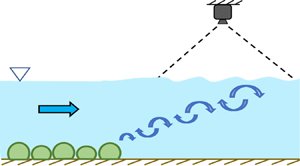
Assessing the surface expression of these submerged features requires measurement of the surface. Various techniques exist to measure either the velocity field on the surface, such as surface particle image velocimetry (Logory, Hirsa & Anthony Reference Logory, Hirsa and Anthony1996; Dabiri & Gharib Reference Dabiri and Gharib2001) and surface particle tracking velocimetry (Sokoray-Varga & Józsa Reference Sokoray-Varga and Józsa2008), the surface slope field, such as free-surface synthetic Schlieren (Mandel et al. Reference Mandel, Rosenzweig, Chung, Ouellette and Koseff2017) and polarimetric slope sensing (Zappa et al. Reference Zappa, Banner, Schultz, Corrada-Emmanuel, Wolff and Yalcin2008; Barsic & Chinn Reference Barsic and Chinn2012), or the free-surface height field, such as Fourier-transform profilometry (Takeda, Ina & Kobayashi Reference Takeda, Ina and Kobayashi1982; Takeda & Mutoh Reference Takeda and Mutoh1983; Cobelli et al. Reference Cobelli, Petitjeans, Maurel and Pagneux2018). For our purposes here, however, such detailed information is not necessary. We, therefore, simply imaged the surface of the flow beginning 15 cm downstream of the bedform patch using an overhead  $1280 \times 1024$ pixel camera mounted along the flume centreline approximately 206 cm from the bottom of the flume. The camera's field of view was approximately 41 cm wide and 44 cm in the streamwise direction. The lighting conditions were similar for all the experiments. To make the free-surface patterns observed in the raw images more pronounced, we subtracted consecutive frames (taken at a rate of 16 frames per second) to create difference images, which were used for all of our analyses. Examples of such difference images are shown for each bottom treatment in figure 2. For each case, we acquired several thousand images.

Figure 2. Sample difference images (as defined in § 2) for the four different bottom treatments for the shallow–fast case. The flow direction is from the bottom to the top of the images.  $(a)$ ‘Canopy’.
  $(b)$ Coral skeletons.
  $(c)$ ‘Dunes’.
  $(d)$ ‘Rocks’.
Finally, since in realistic environmental situations there will typically be more surface disturbances present than just those arising from bathymetric features, we also conducted a set of experiments using a fan to produce wind ruffles on the free surface. For these cases, the flow Reynolds number was kept constant at  $Re_H = 55.1\times 10^3$ (the fast case), but both the submergence and the wind speed were varied. We tested three different wind speeds:
  $1.6\ \textrm {m}\,\textrm {s}^{-1}$,
  $2.2\ \textrm {m}\,\textrm {s}^{-1}$ and
  $2.6\ \textrm {m}\,\textrm {s}^{-1}$, as measured 2 cm above the water surface at a distance of 37 cm from the end of the bedform patch using a hot-wire anemometer probe. The amplitude of the surface disturbances produced by the wind varied somewhat with wind speed, but in all cases was similar to or smaller than the disturbances produced by the bottom treatments. Examples of difference images in the presence of wind are shown for each bottom treatment in figure 3.

Figure 3. Sample difference images in the presence of wind (at wind speed  $2.6\ \textrm {m}\,\textrm {s}^{-1}$ as defined in § 2) for the four different bottom treatments for the shallow–fast case. The flow direction is from the bottom to the top of the images.
  $(a)$ ‘Canopy’.
  $(b)$ Coral skeletons.
  $(c)$ ‘Dunes’.
  $(d)$ ‘Rocks’.
3. Analysis framework
To analyse the images of the free surface, we used a classifier based on a CNN. The details of the CNN (namely the architecture and the hyperparameters) are provided in the Appendix. Here, we describe the three key steps in the analysis pipeline.
The first step was to train the CNN to distinguish images associated with each of the different bedforms. To do so, we fed the CNN images associated with each of the bedforms over a variety of flow conditions. Note that these training images were only a subset of the full ensemble of images acquired. The training images were labelled with the bedform class (i.e. canopy, coral, dunes or rocks), but not with the flow conditions. During the iterative process of learning the decision boundaries between the classes, the CNN minimizes the loss between the predicted label for a training image and its true label. In this way, the classifier learns features of interest from the images that help it classify them with high accuracy. Note that we use the term ‘accuracy’ in this case to mean the percentage of the images given to the CNN that were classified correctly.
Once the model was trained, we tested its ability to classify a set of images that belonged to the same flow conditions as those in the training set but were not seen by the model during training. This training-development set was used to validate the ability of the CNN to classify images that it had not seen but were acquired under the same conditions used during the training phase. High accuracy on this set indicates that the model is not overfit to the training images.
The final step was to use the CNN to classify a test set of images acquired under flow conditions that it has not been trained on. This step allows us to determine the confidence with which the CNN can classify images based on the information it has learned during the training phase.
The precise sizes of the image sets used for the different cases discussed below varied, but in all cases were empirically determined to be large enough to give stable results. The training sets ranged from 24 000 to 48 000 images; the training-development sets from 1200 to 1600 images; and the test sets from 4800 to 8000 images. In all cases, equal numbers of images were used for each of the four bottom treatments.
4. Results and discussion
4.1. Classification of bedforms without wind
To examine whether a measurable signature of the different bedforms was present at the free surface, we trained nine different CNNs on sets of images acquired from flows with different bedforms and flow conditions but no wind ruffles. The nine CNNs differed in that their training and training-development sets consisted of images taken for all four bedform types but only eight of the nine different flow configurations. The images for the remaining flow condition (but again for all four bedforms) constituted the test set.
The accuracy of these nine CNN classifiers is shown in table 1. Each ( $Re_H, \mathcal {S}$) pair in the table denotes the flow condition that was held out of the training set and instead taken as the test set. For each classifier, we show the accuracy separately for the training set (in italic), training-development set (in bold) and test set (in bold italic). For example, for the classifier for which the medium
  $Re_H$ and intermediate
  $\mathcal {S}$ flow case images were held out from the training, the training set accuracy was
  $99.3\,\%$, the training-development set accuracy was
  $98.0\,\%$, and the test set accuracy was
  $87.8\,\%$. Note that, by construction, all the test cases consist of images of flow conditions that the CNNs were not exposed to during training, rendering classification a non-trivial task. Nevertheless, all nine CNNs perform significantly better than random chance, which would give an accuracy of
  $25\,\%$. This result suggests that the CNNs have indeed learned to pick out informative features from the images of the free surface that accurately identify characteristics of the bottom bathymetry, giving strong evidence that such surface signatures exist.
Table 1. Per cent accuracy of the nine CNN classifiers discussed in § 4.1. Each of the nine ( $Re_H, \mathcal {S}$) pairs in the table corresponds to a different model, and its placement in the table indicates the flow condition that was held out from the training set and used for testing instead. For each classifier, the training set accuracy, training-development set accuracy and test set accuracy are shown in italic, bold and bold italic, respectively.

However, the test accuracy of the CNNs in classifying images for some of the flow conditions is far from perfect. To analyse this result in more detail, we computed the confusion matrices (Pedregosa et al. Reference Pedregosa, Varoquaux, Gramfort, Michel, Thirion, Grisel, Blondel, Prettenhofer, Weiss and Dubourg2011), shown in figure 4. These matrices report the fraction of the test set images corresponding to one kind of bedform that were classified as another for all pairs. These confusion matrices reveal that low overall accuracy does not result from across-the-board poor performance. Instead, for example, for the case of slow, shallow flow (figure 4a), rocks are consistently misclassified as dunes, but never as corals or canopy. Similarly, corals are misclassified as dunes  $69\,\%$ of the time. Dunes and canopies themselves, however, are well classified by the same CNN. Therefore, poor classification for some of the bedforms results in a lower overall accuracy (e.g.
  $52.3\,\%$ test set accuracy for the slow, shallow flow case of figure 4a). In contrast, there are also flow cases (such as fast, intermediate-depth flow; see figure 4f) where the CNN performs excellently for all of the bedforms.

Figure 4. Confusion matrices for the test-set performance of the nine classifier models discussed in § 4.1. The numbers in each of the boxes give the fraction of test images belonging to a particular bedform (row labels) that are classified by the CNN as belonging to one of the four bedforms (column labels).  $(a)$ Shallow flow, slow flow-rate holdout.
  $(b)$ Shallow flow, medium flow-rate holdout.
  $(c)$ Shallow flow, fast flow-rate holdout.
  $(d)$ Intermediate-depth flow, slow flow-rate holdout.
  $(e)$ Intermediate-depth flow, medium flow-rate holdout.
  $(\,f)$ Intermediate-depth flow, fast flow-rate holdout.
  $(g)$ Deep flow, slow flow-rate holdout.
  $(h)$ Deep flow, medium flow-rate holdout.
  $(i)$ Deep flow, fast flow-rate holdout.
4.2. Classification in the presence of wind
In actual environmental flows of interest, distortions of the free surface will arise both from bottom features and from stresses applied directly at the surface by phenomena such as wind. One might anticipate that if these direct surface effects are strong enough, they will overwhelm the surface signature of any bottom features. To explore this hypothesis, we conducted a series of experiments where we introduced surface winds over the flume (as described in § 2) and again used CNNs to attempt to classify the bottom features. We did this in two ways. First, we trained a CNN classifier only on images taken for flows with no imposed wind and tested its performance on experimental cases with imposed winds. And second, we trained classifiers with images that did include imposed winds, in a manner similar to that described above in § 4.1.
4.2.1. Classifiers trained on flows without wind
For the first of these cases, we trained a single CNN classifier using images taken from the full set of nine flow conditions described above (varying Reynolds number and submergence), and tested its performance separately for each of the three imposed wind-speed conditions ( $1.6\ \textrm {m}\,\textrm {s}^{-1}$,
  $2.2\ \textrm {m}\,\textrm {s}^{-1}$ and
  $2.6\ \textrm {m}\,\textrm {s}^{-1}$). Note that, as mentioned above, the Reynolds number was kept constant for each wind speed, but images were acquired for all three submergences.
The performance of the CNN in classifying the images in these test cases was significantly degraded by the presence of surface disturbances due to the wind: we found that the accuracy of the classifier was  $33\,\%$,
  $35\,\%$ and
  $36\,\%$ for wind speeds of
  $1.6\ \textrm {m}\,\textrm {s}^{-1}$,
  $2.2\ \textrm {m}\,\textrm {s}^{-1}$ and
  $2.6\ \textrm {m}\,\textrm {s}^{-1}$, respectively. Although these accuracies are still better than random chance, they are far lower than those found for experiments without imposed wind (§ 4.1).
Insight into why the performance was so poor can be gleaned from the confusion matrices, as shown in figure 5. They reveal that the accuracy of the CNN is low because almost all cases are classified as dunes, regardless of the actual bedform. This result is not necessarily surprising. As described in § 2, the fan that generated the wind was oriented along the centreline of the flume; thus, one would expect that the dominant features produced by the wind would be surface waves spanning the width of the flume with their crests oriented along the spanwise direction. Of the four model bedforms used, only our model dunes shared this symmetry. Thus, it would appear that the CNN, as trained on images with no wind, learned that the surface signature of dunes involves features with a geometry shared by the features produced by wind – and thus consistently tended to classify windy images as dunes.

Figure 5. Confusion matrices for the three different wind-speed test cases discussed in § 4.2.1. No images taken with imposed surface winds were used to train the CNN used for these cases.  $(a)$
$(a)$ $\text {Wind speed} = 1.6\ \textrm {m}\,\textrm {s}^{-1}$.
  $(b)$
$(b)$ $\text {Wind speed} = 2.2\ \textrm {m}\,\textrm {s}^{-1}$.
  $(c)$
$(c)$ $\text {Wind speed} = 2.6 \ \textrm {m}\,\textrm {s}^{-1}$.
4.2.2. Classifiers trained on flows with wind
To establish whether wind unavoidably destroys the possibility of classifying bottom features or whether instead different features must be used to discriminate between the types of bedforms, we next trained two CNNs on training sets that included images taken from cases with wind in addition to cases without wind. As in § 4.1, for each CNN classifier, we held out one data set from the training set of images to use as the test set.
For the first classifier, the test set was the case of intermediate submergence ( $\mathcal {S} = 1.5$), medium Reynolds number (
 $Re_H = 43.7\times 10^3$) and no wind. This case allowed us to assess how much, if at all, the addition of images with wind degraded the ability of the CNN to classify cases without wind. The accuracy for this case was
  $75\,\%$, lower than that described above for cases without wind, but still far above random chance.
For the second classifier, the test set was the case of intermediate submergence, high Reynolds number ( $Re_H = 55.1\times 10^3$) and a wind speed of
  $2.2\ \textrm {m}\,\textrm {s}^{-1}$. In this case, the accuracy of the CNN was
  $86\,\%$ – significantly better than the performance of CNNs trained without exposure to training images containing wind.
Taken together, these tests suggest that although the presence of imposed surface disturbances due to wind adds additional complexity to the classification problem, they do not eliminate the surface signature of the bedforms. This result is consistent with the findings of Rosenzweig (Reference Rosenzweig2017), who showed that the modification of the near-surface velocity spectra by a submerged canopy was evident even in the presence of an imposed wind chop. Thus, we conclude that the surface signature of submerged features can persist in a distinguishable way even when the surface is directly acted upon by other physical processes.
5. Conclusion
The results we have presented give strong evidence that the free-surface disturbances caused by submerged features can carry sufficient information to identify at least the gross characteristics of the feature. We have also shown that although directly imposed surface disturbances, such as winds, may also modulate the free surface, they do not necessarily preclude the identification of the submerged feature provided that appropriate information is used.
These results point to a number of intriguing questions for future research. For example, how far downstream of a bedform do signatures typically manifest, how quickly do they decay, and what physics governs these processes? We speculate, for instance, that the poorer test performance for the shallow-slow flow case in table 1 may be a result of the measurement region being too far from the bedform so that surface fluctuations indicative of the bedform will have decayed by the time they are imaged. Further study of the mechanisms by which information is generated at the bed and propagates to the surface may also clarify the range of flow conditions over which one may expect bathymetry inference to be possible. For example, if the flow were completely laminar, there would be no reason to expect significant fluctuations due to interaction between the bedform and the flow and, therefore, there would be no surface signature of the bedform. In the other extreme, if the flow were extremely turbulent, potential bedform signatures on the free surface may be washed out by the ambient turbulent fluctuations.
Because we only used CNNs in this study, we cannot definitively address these questions of physical mechanism: our work suggests the existence of a connection between the submerged feature and the surface expression, but not the nature of that connection. To answer the questions posed above in detail requires different tools, such as those discussed in § 2, that allow the spatiotemporal reconstruction of the free-surface elevation or slope. Nevertheless, our demonstration that this bathymetry inference is possible presents a strong motivation for conducting future studies that directly probe the physical processes responsible for transporting information about the bottom of the flow to the surface.
Acknowledgements
S.G. gratefully acknowledges the support of The Link Foundation Ocean Engineering and Instrumentation Ph.D. fellowship. We also acknowledge funding from the Stanford Woods Institute for the Environment. We thank T. L. Mandel for assistance with the experimental facilities and A. Pal and S. Arslan for input on the CNN models.
Declaration of interests
The authors report no conflict of interest.
Appendix. CNN architecture
Our CNN based classifiers were built using the Keras library (Chollet et al. Reference Chollet2015) that uses tensorflow-v2 (Abadi et al. Reference Abadi, Barham, Chen, Chen, Davis, Dean, Devin, Ghemawat, Irving and Isard2016) as its backend. Our CNN architecture is illustrated in figure 6. We stacked four  $\{$convolution + relu + maxpooling
 $\}$ modules followed by two fully connected layers. Convolution filters operated on
  $16\times 16$,
  $10\times 10$,
  $5\times 5$ and
  $3\times 3$ windows with a stride of 1 and the ‘same’ padding. Our maxpooling layers operated on
  $2\times 2$ windows with a stride of 2. There were 16, 16, 32 and 64 filters, respectively, for each convolutional layer. We trained the model with the categorical cross-entropy loss because we are solving a multi-class classification problem. Last layer activation was softmax, so that the output of the model for a given image can be interpreted as the probability that an image belongs to a given class. For model optimization during training, we used the RMSProp optimizer with a learning rate of 0.001 and a training batch size of 50 images with accuracy as the guiding metric. Training was carried out for 30 epochs. All images fed into this model were rescaled to
  $224\times 224$ pixels. When building the training and training-development sets, we randomly shuffled the difference images so as not to inadvertently include temporal correlations.

Figure 6. The CNN architecture used for this study.


