2.1. Inviscid attached flow

The streamfunction for attached flow and $d=0$ is developed in Milne-Thomson (Reference Milne-Thomson1996) § 9.63, page 258. For general $d$, in the (non-inertial) frame of reference, the streamfunction can be written as

(2.2)\begin{equation} \psi(x,y,t) = {\textrm{Im}}\left\{W_a(z,t)\right\}-{\tfrac{1}{2}}\varOmega(t) (x^2+y^2),\end{equation}

where $z = x + \textrm {i} y$ with $\textrm {i}$ being the imaginary unit, and

(2.3a)\begin{gather} W_a(z,t) = \frac{A(t)}{\zeta} + \frac{B(t)}{\zeta^2} + U(t) (z + a d) \exp(-\textrm{i}\alpha(t)), \end{gather}

(2.3b)\begin{gather}A(t) = \textrm{i} a [-a \varOmega(t) d + U(t) \sin(\alpha(t))],\quad B(t) = \frac{\textrm{i}}{4} \varOmega(t) a^2, \end{gather}

(2.3c)\begin{gather}\zeta(z) = \frac{z}{a}+d + \left( \frac{z}{a}+d -1 \right)^{{1}/{2}} \left(\frac{z}{a} +d+1 \right)^{{1}/{2}}, \end{gather}

where the time dependence is due only to the plate's kinematics in this inviscid formulation. The subscript of $W_a$ refers to attached flow, $\zeta (z)$ maps the exterior of the flat plate located at $C \equiv \{ z = x + \textrm {i} y \,|\, -a (1+d)\le x \le a (1-d)\ \text {and}\ y=0 \}$, to the exterior of the unit circle, $\mathcal {C} \equiv \{ \zeta = \xi + \textrm {i}\eta \,|\,|\zeta |=1\}$. An appropriate branch can be defined by a cut connecting the branch points, $z = (-a [1+d],0)$ and $(a [1-d],0)$. The points, $\zeta = (-1,0)$ and $(1,0)$, map to the plate edges at $z = (-a [1+d],0)$ and $(a [1-d],0)$, respectively. On $\mathcal {C}$, $\zeta = \exp (\textrm {i} \chi )$ maps to the plate surface, $z = a (\cos \chi -d)$. It is easily verified that on the plate, the streamfunction is $\psi = - {\frac {1}{4}} a^2 \varOmega (1+2 d^2)$ which depends on time only. Streamlines are shown in figure 2 for translational speed, $U=1$, angular speed, $\varOmega =3$, pivot position at the plate centre, $d=0$ and angle of attack, $\alpha = {\rm \pi}/4$.

Figure 2. Streamlines generated by a flat rigid plate with $a=1$, $U=1$, $\varOmega =3$, $d=0$ and $\alpha = {\rm \pi}/4$, corresponding to a plate of length 2, instantaneous translational speed of 1, rotating with instantaneous angular speed of 3, pivot point at the plate centre and instantaneous angle of attack of ${\rm \pi} /4$, respectively. Streamlines shown in reference frame of the moving plate.

In the translating and rotating reference frame of the plate, the velocity components at a field point, $z$, can be written as

(2.4)\begin{equation} u-\textrm{i} v = \frac{\textrm{d} W_a}{\textrm{d} z}-\textrm{i}\varOmega \bar{z},\end{equation}

where the overline denotes the complex conjugate. The vorticity is zero.

In this reference frame, the $x$ and $y$ fluid velocity components at the plate surface are, respectively,

(2.5a,b)\begin{equation} u = \frac{a\varOmega[d \cos\chi - {\frac{1}{2}} \cos(2 \chi)] -U\sin (\alpha-\chi)}{\sin{\chi}},\quad v =0. \end{equation}

Generally, $u$ is singular at the plate trailing edge $\chi =0$ (i.e. $z=a [1-d]$) and leading edge $\chi = {\rm \pi}$ (i.e. $z = -a [1+d]$). A stagnation point on the plate surface occurs when $u=0$, giving

(2.6)\begin{equation} a\varOmega [d \cos\chi - \tfrac{1}{2} \cos(2 \chi)] -U\sin (\alpha-\chi)=0.\end{equation}

When $d=0$, $U=0$, $\varOmega \ne 0$ (pure rotation about the plate centre), stagnation points occur at $\cos (2 \chi )=0$ and so $\chi = {\rm \pi}/4$, $3{\rm \pi} /4$, $5{\rm \pi} /4$, $7{\rm \pi} /4$. This corresponds to $x = \pm a/\sqrt {2}$, $y =0^+$ and $0^-$, in agreement with Milne-Thomson (Reference Milne-Thomson1996).

2.2. Attached flow near the trailing edge

The function, $W_a(z,t)$, has a $(z/a+ d-1)^{{1}/{2}}$ singularity at the trailing edge, $z =a (1-d)$, where for attached flow, the fluid velocity and pressure are both singular. We consider spatial points near $z =a (1-d)$ and write

(2.7a,b)\begin{equation} z = a (1-d) + \hat{z},\quad \hat{z} = \hat{x} + \textrm{i}\hat{y} = r \exp(\textrm{i} \theta),\end{equation}

where $r = \sqrt { \hat {x}^2 + \hat {y}^2}$ and $\theta \in [-{\rm \pi} , {\rm \pi})$ is the angle made by $\hat {z}$ with the positive $\hat {x}$-axis. Expanding $W_a(z,t)$ for small $r$, and any term that is purely a function of time (including constants), gives

(2.8)\begin{align} W_a(\hat{z}) &= -2\,i\,\left(\frac{a}{2}\right)^{1/2} \hat{z}^{1/2} \left(a\varOmega \left[{\frac{1}{2}}-d\right]+ U\sin\alpha \right) \nonumber\\ &\quad + \hat{z}\left(\textrm{i}a\varOmega [1-d] + U \cos\alpha \right) + {O}(\hat{z}^{3/2}). \end{align}

The branch cut for $\hat {z}^{1/2}$ extends from $\hat {z}=0$ along the negative $\hat {x}$ axis, i.e. along the plate. Using (2.4), the complex velocity for the attached flow (again denoted with subscript, $a$) near the trailing edge is

(2.9)\begin{equation} u_a-\textrm{i} v_a = -\textrm{i}\left(\frac{a}{2}\right)^{1/2} \hat{z}^{-1/2}\left(a\varOmega \left[{\frac{1}{2}}-d\right] + U\sin\alpha \right) + U\cos\alpha + {O}(|\hat{z}|^{1/2}).\end{equation}

For rotation about the three-quarter chord point, $d=1/2$, the rotational contribution to (2.9) vanishes. More generally, it can be seen that the coefficient of $\hat {z}^{-1/2}$ is zero when $a\varOmega (1/2-d) +U\sin \alpha =0$. Streamlines for a flow with this property are shown in figure 3 for translational speed, $U=3/(2\sqrt {2})$, angular speed, $\varOmega =3$, rotation about the three-quarter chord point, $d=1/2$, and angle of attack, $\alpha = {\rm \pi}/4$. The plate lies on the interval, $-3/4\le x \le 1/4$ and $y=0$. It can be seen that there is smooth flow off the trailing edge, $z =x + \textrm {i} y = 1/4$. This condition will be instantaneous at $t= 0^+$.

Figure 3. Streamlines generated by a flat rigid plate with $a=1$, $U=3/(2\sqrt {2})$, $\varOmega =3$, $d=1/2$ and $\alpha = {\rm \pi}/4$. (a) Full-plate view. (b) Close up near trailing edge. These parameters are similar to those used for the flow in figure 2, except the plate now rotates about its three-quarter chord point (rather than its centre) and has a translational speed of $U=3/(2\sqrt {2})\approx 1.06$ (rather than 1). Streamlines again shown in the moving reference frame of the plate.

2.3. Power law in time motion of the plate

We consider a plate whose respective translational and rotational speeds are

(2.10a,b)\begin{equation} U(T) = U_0 T^m,\quad \varOmega(T) = \varOmega_0 T^p,\end{equation}

where $U_0>0$ and $\varOmega _0>0$ are the (constant) characteristic translational and angular velocity scales, respectively, and dimensionless time is

(2.11)\begin{equation} T = \frac{t U_0}{a}.\end{equation}

The constants, $m \ge 0$ and $p \ge 0$, in (2.10a,b) are key control parameters of the plate motion that specify its translational and rotational time dependencies, respectively.

The instantaneous angle of attack, $\alpha (T)$, of the plate directly follows from (2.10a,b),

(2.12)\begin{equation} \alpha(T) = \alpha_0 + \frac{\beta}{1+p}T^{1+p},\end{equation}

where $\alpha _0$ is the initial angle of attack. The constant parameter,

(2.13)\begin{equation} \beta = \frac{\varOmega_0 a}{U_0},\end{equation}

specifies the relative rotational-to-translational plate motion.

Impulsive pure rectilinear motion at constant angle of attack, $\alpha (t) = \alpha _0$, corresponds to $m=0$ (giving $U =U_0 > 0$) and $\varOmega _0 \to 0$ (Prandtl Reference Prandtl1924); this widely studied case is discussed in § 5.6.

3.1. Self-induced velocity of vortex sheet

In the complex $z$-plane, we describe the separated vortex-sheet position and motion by the function $\hat {z} = \hat {z}_v(\varGamma ,t)$, where $\varGamma$ is a Lagrangian-like variable that measures the total amount of circulation between a point on the vortex sheet and its free edge; the subscript $v$ refers to the vortex sheet. For a material point on the sheet, moving with the average of the field velocities on either side of the sheet, $\varGamma$ is conserved. The dynamical motion of the sheet is described by the Eulerian–Lagrangian Birkhoff–Rott equation (Rott Reference Rott1956; Birkhoff Reference Birkhoff1962; Saffman Reference Saffman1992)

(3.1)\begin{equation} \left(\frac{\partial \bar{\hat{z}}_v}{\partial t}\right)_{\varGamma} = u_a-\textrm{i} v_a + u_{v}-\textrm{i} v_{v}, \end{equation}

where $u_{v}-\textrm {i} v_{v}$ is the self-induced, sheet-image velocity that satisfies the boundary condition on the plate, guaranteeing total circulation of the vortex–plate system is zero. Using the image-circle theorem (Milne-Thomson Reference Milne-Thomson1996) to construct an image system in the circle in the $\zeta$-plane, that satisfies the boundary condition of zero normal velocity on the flat plate with zero total circulation, this velocity contribution can be expressed as

(3.2)\begin{equation} u_{v}-\textrm{i}v_{v} = - \left(\frac{\textrm{d}\zeta}{\textrm{d} z}\right)_{\hat{z}_v} \frac{1}{2 {\rm \pi}\textrm{i}} \int\kern-10pt^0_{\varGamma_0(t)} \left( \frac{1}{\zeta_v -\zeta'_v} - \frac{1}{\zeta_v-\dfrac{1}{\bar{\zeta}'_v}} \right) \textrm{d}\varGamma',\end{equation}

where $\zeta _v(\varGamma ,t)=\zeta (z_v(\varGamma ,t))$ is the vortex-sheet curve in the $\zeta$-plane given by (2.3c) and $\zeta _v'=\zeta (z_v(\varGamma ',t))$. In (3.2), the integral denotes the Cauchy principal value. The upper limit of integration corresponds to the vortex-sheet free edge which is the point on the sheet that began the separation at $t=0$; the lower limit of $\varGamma _0(t)$ is the total circulation shed at time $t>0$ and coincides with the plate trailing edge. The first term inside the integral represents the self-induction of the shed vortex sheet while the second term is the complex velocity induced by the image vortex sheet, or ‘bound’ circulation.

Using (2.3c) to expand the integrand in (3.2) to leading order for $| \hat {z}_v | \ll a$, and substituting the result and (2.9) into (3.1), gives the required dynamical equation describing the vortex-sheet motion to $ {O}(\hat {z}_v^{1/2})$,

(3.3)\begin{align} \left(\frac{\partial \bar{\hat{z}}_v}{\partial t}\right)_{\varGamma} &= U \cos\alpha -\textrm{i}\left(\frac{a}{2}\right)^{1/2} \hat{z}_v^{-1/2} \left(a \varOmega \left[{\frac{1}{2}}-d\right] + U \sin\alpha \right) \nonumber\\ &\quad -\frac{1}{4 {\rm \pi}\textrm{i}} z_v^{-1/2} \int\kern-10pt^0_{\varGamma_0(t)} \left(\frac{1}{z_v^{1/2} -{z'_v}^{1/2}}-\frac{1}{z_v^{1/2} +\overline{z'_v}^{1/2}} \right) \textrm{d}\varGamma'. \end{align}

The Kutta condition, that the complex velocity at the plate edge is always finite, can be obtained by taking the limit, $\hat {z}_v\to 0$. Requiring that the coefficient of the singular term on the right-hand side vanishes then gives

(3.4)\begin{equation} \frac{1}{4 {\rm \pi}} \int^0_{\varGamma_0(t)} \left( \frac{1}{{z_v}^{1/2}} + \frac{1}{\overline{z_v}^{1/2}} \right) \textrm{d}\varGamma +\left(\frac{a}{2}\right)^{1/2} \left(a \varOmega \left[{\frac{1}{2}}-d\right] + U \sin\alpha \right) =0. \end{equation}

It can be seen that both (3.3) and (3.4) contain the term, $a \varOmega [{\frac {1}{2}}-d] + U \sin \alpha$, where the time dependence of $\varOmega$, $U$ and $\alpha$ have been omitted. This term is generally non-zero at $t=0$. However, if it vanishes at $t=0$, then for non-zero $U(t)$, it cannot remain at zero for all $t > 0$. The special limiting case, $\varOmega (t) \to 0$ and $\alpha (t) \to 0$, corresponds to no starting vortex because the Kutta condition is automatically satisfied; see § 5.6 for a general discussion of the zero rotation limit.

4.1. Formulation

Motivated by specified time dependencies of the plate motion in (2.10a,b) and (2.12), and hence the flow boundary conditions, we search for similarity solutions for the vortex sheet of the form

(4.1a,b)\begin{equation} \frac{\hat{z}_v}{a} = T^q Z(\lambda),\quad \lambda = 1 - \frac{1}{\mathcal{J} T^s} \frac{\varGamma}{U_0 a},\end{equation}

where $q\ge 0$ and $s\ge 0$ are additional power-law constants and $\mathcal {J}$ is a dimensionless constant related to the total shed circulation (see (4.3)), all of which are to be determined. The form of the second equation in (4.1a,b) is now justified.

In (4.1a,b), $\lambda$ is a similarity parameter defined to take the value $\lambda =0$ at the plate trailing edge (point of separation), i.e.

(4.2)\begin{equation} Z(0) = 0, \end{equation}

while $\lambda =1$ corresponds to the vortex-sheet free edge. The circulation, $\varGamma$, is constant at any material point on the vortex sheet; see § 3.1. Defining $\varGamma _0 (T)= \varGamma$ at the plate trailing edge ($\lambda =0$), from (4.1a,b) it then follows that the total shed circulation is

(4.3)\begin{equation} \varGamma_0(T) = U_0 a \mathcal{J} T^s, \end{equation}

where $\mathcal {J}$ is henceforth termed the ‘shed circulation constant’.

Substitution of (4.1a,b) into (3.3) and (3.4) and utilizing (2.13) and (2.10a,b) gives, after some algebra

(4.4)\begin{align} T^{q-1} \left(q \bar{Z} + s (1-\lambda) \frac{d \bar{Z}}{d \lambda}\right) &= T^m \cos \left(\alpha_0+\frac{\beta}{1+p} T^{1+p}\right)\nonumber\\ &\quad - \frac{\textrm{i}}{ Z^{1/2}} \left( \frac{1}{2^{1/2}} T^{-q/2} \tilde{Q}(T) + \frac{\mathcal{J}}{4 {\rm \pi}} T^{s-q} I(Z)\right), \end{align}

where

(4.5a)\begin{gather} I(Z)= \int^1_0\kern-14pt - \left( \frac{1}{Z^{1/2} -{Z'}^{1/2}} - \frac{1}{ Z^{1/2} +\overline{Z'}^{1/2}} \right) \textrm{d}\lambda', \end{gather}

(4.5b)\begin{gather}\tilde{Q}(T) = T^p \beta \left({\frac{1}{2}}-d\right) + T^m \sin \left(\alpha_0+\frac{\beta}{1+p} T^{1+p}\right), \end{gather}

and the Kutta condition becomes

(4.6)\begin{equation} \frac{\mathcal{J}}{4 {\rm \pi}} T^{s-q/2}\int^1_0 \left( \frac{1}{Z^{1/2} } + \frac{1}{\bar{Z}^{1/2}} \right) \textrm{d}\lambda = \frac{1}{2^{1/2}} \tilde{Q}(T),\end{equation}

where $Z' \equiv Z(\lambda ')$. The left-hand side of (4.4) is the time derivative on the left-hand side of (3.3). The first term on the right-hand side is the convective free stream, while the two terms in brackets on the right-hand side are respectively the singular attached flow and the vortex-sheet induced velocity.

Equation (4.4) forms the basis of our analysis of the starting vortex. The control parameters are $(m,p,\alpha _0,d,\beta )$ which are to be specified; see start of § 3 for their physical meaning.

4.2. Dominant-balance analysis

As discussed in § 1, our focus is on the primitive start-up vortex. We thus consider the limit of small convective time, $T$, when performing a dominant-balance analysis of (4.4)–(4.6). In seeking a time-dependent solution, the unsteady term on the left-hand side of (4.4) must be retained because it represents the highest-order time derivative in the system. We now search for dominant terms on the right-hand side that will balance the unsteady term in powers of $T$ in the limit $T\to 0^+$. Owing both to the structure of $\tilde {Q}(T)$ in (4.5b) which contains two terms, and also the trigonometric functions of $\alpha (T)$ in (4.4) and (4.5b), which also have two terms, different scenarios must be considered.

The parameter space can be explored with four distinct plate motions: (a) $\alpha _0 =0$ with (i) $d\ne 1/2$ and (ii) $d = 1/2$; (b) $\alpha _0 \ne 0$ with (i) $d\ne 1/2$ and (ii) $d = 1/2$. Starting flows with $d=1/2$ (rotation about the three-quarter chord point) may differ from those with $d\ne 1/2$ because for the former, the coefficient of $\beta$ in (4.5b) is zero. Likewise flows with non-zero initial angle of attack, i.e. $\alpha _0 \ne 0$, will have different start-up behaviour from those with $\alpha _0 = 0$. The latter will be seen to be delicate because the trailing-edge singularity can take a weak form. In the following, we consider these four classes by obtaining the relevant power-law growth of both the starting-vortex trajectory and circulation.

In the next section, a detailed solution of the flow generated by the first distinct plate motion, $\alpha _0=0$ with $d \ne 1/2$, corresponding to zero initial angle of attack and rotation away from the plate three-quarter chord position, respectively, is developed together with sample numerical solutions; see § 5.1. For brevity, cursory analyses of the other three distinct plate motions are presented in §§ 5.2–5.4 with details and numerical case studies left to the reader.

5.1. $\alpha _0 = 0$, $d\ne 1/2$

This first distinct plate motion produces the most novel starting-vortex dynamics and is documented in detail in this section. Here, the second term in $\tilde {Q}(T)$ in (4.5b), of order $T^{1+m+p}$, can always be neglected compared to the first term. Further, we can take $\cos (\alpha (t)) =1 + {O}(T^{2(1+p)}) =1$ to the order required. To leading order, the Kutta condition (4.6) is then

(5.1)\begin{equation} \frac{\mathcal{J}}{4 {\rm \pi}} T^{s-q/2} \int^1_0 \left(\frac{1}{Z^{1/2} } + \frac{1}{\bar{Z}^{1/2}} \right) \textrm{d}\lambda = \frac{1}{2^{1/2}} T^p \hat{\beta}, \end{equation}

where the following composite parameter naturally emerges,

(5.2)\begin{equation} \hat{\beta} = \beta \left({\tfrac{1}{2}}-d\right). \end{equation}

For finite shed circulation, (5.1) requires

(5.3)\begin{equation} s = q/2+p. \end{equation}

The parameter $p$, defined in (2.10a,b), is a key control parameter specifying rotational motion of the plate, whereas $q$ and $s$ describe the vortex motion and are to be determined. Equation (4.4) therefore becomes

(5.4)\begin{equation} T^{q-1} \left(q \bar{Z} + (q/2+p) (1-\lambda) \frac{\textrm{d} \bar{Z}}{\textrm{d} \lambda}\right) = T^m - T^{-q/2+p} \frac{\textrm{i}}{Z^{1/2}} \left(\frac{1}{2^{1/2}} \hat{\beta} +\frac{\mathcal{J}}{4 {\rm \pi}} I(Z)\right). \end{equation}

We consider three separate cases for the primitive start-up vortex, i.e. for $T\ll 1$, which we denote Type I, Type II and Type III, respectively.

5.1.1. Type I vortex sheet

We first examine when rotational motion of the plate dominates convection due to its translation. For kinematic reasons, we expect the vortex-sheet roll-up centre to be shed (approximately) normal to the plate's trailing edge. This corresponds to a dominant balance between the left-hand side and the second term on the right-hand-side of (5.4). Equating powers of $T$ and using (5.3) gives $q = 2 (1+p)/3$ and $s = (4 p+1)/3$. For the first term on the right-hand side of (5.4) to remain subdominant, we require $m>q-1$, i.e. $m > (2 p-1)/3$. Substituting these results into (4.1a,b) and (4.3) provides the required solution,

(5.5a,b)\begin{equation} \frac{\hat{z}_v}{a} = T^{{2 (1+p)}/{3}} Z(\lambda),\quad \tilde{\varGamma}\equiv \frac{\varGamma_0(T)}{U_0 a} = \mathcal{J} T^{{(1+4 p)}/{3}},\quad \text{for}\ m> \frac{2 p-1}{3},\end{equation}

where $Z(\lambda )$ and the shed circulation constant, $\mathcal {J}$, are now determined by the integro-differential equation (IDE) obtained by retaining the dominant terms in (5.4),

(5.6)\begin{equation} \frac{2}{3} (1+p)\left(\bar{Z} +\frac{4 p+1}{2 (p+1)} (1-\lambda) \frac{\textrm{d} \bar{Z}}{\textrm{d} \lambda}\right) =-\frac{\textrm{i}}{Z^{1/2}}\left( \frac{1}{2^{1/2}} \hat{\beta} +\frac{\mathcal{J}}{4 {\rm \pi}} I(Z) \right), \end{equation}

subject to the initial condition, (4.2), and the Kutta condition

(5.7)\begin{equation} \mathcal{J} \int^1_0 \left( \frac{1}{Z^{1/2} } +\frac{1}{\bar{Z}^{1/2}} \right) \textrm{d}\lambda = 2 \sqrt{2} {\rm \pi}\hat{\beta}. \end{equation}

The change of variables

(5.8a,b)\begin{equation} \mathcal{J} = A J,\quad Z = B \omega, \end{equation}

where

(5.9a,b)\begin{equation} A = \left(\frac{3 \hat{\beta}^4}{1+p} \right)^{{1}/{3}},\quad B = \frac{1}{2} \left(\frac{3 \hat{\beta}}{1+p} \right)^{{2}/{3}}, \end{equation}

maps (5.6) and (5.7) into (35) and (36) of Pullin (Reference Pullin1978) (with $n=1/2$), reproduced here as

(5.10)\begin{equation} \bar{\omega} +\frac{4 p+1}{2 (p+1)} (1-\lambda) \frac{\textrm{d} \bar{\omega}}{\textrm{d} \lambda} = -\frac{\textrm{i}}{\omega^{1/2}} \left(1 +\frac{J}{2 {\rm \pi}} I(\omega)\right), \end{equation}

with $\omega (0) = 0$ (see (4.2) and (5.8a,b)) and the Kutta condition is

(5.11)\begin{equation} \frac{J}{2 {\rm \pi}} \int^1_0 \left( \frac{1}{\omega^{1/2}} + \frac{1}{\bar{\omega}^{1/2}} \right) \textrm{d}\lambda = 1, \end{equation}

which eliminates the composite parameter, $\hat {\beta }$.

5.1.2. Numerical method

Numerical solutions displayed in figure 9(a) of Pullin (Reference Pullin1978) show the starting-vortex shape in the $\omega$ variable corresponding to Type I starting vortices. The solution for impulsive start up was later independently verified by Jones (Reference Jones2003). Solutions are re-calculated here using the numerical method of Pullin (Reference Pullin1978), for which we now provide a brief summary. The vortex sheet is divided into two parts. The first is a continuous section in $0\le \lambda \le \lambda _N$ represented by $N$ straight segments with the first segment joined to the plate trailing edge. The second is an inner section modelled by a point vortex of strength, $J (1-\lambda _N)$, located at $\omega = \omega _{N+1}$ that is joined to the end of the continuous section by a cut in the $\omega$-plane from $\omega (\lambda _N)$ to $\omega _{N+1}$. A finite-difference form of the IDE in (5.10) is satisfied at the midpoint of each segment of the continuous sheet using a two-point rule for derivatives and a trapezoidal rule for the Cauchy principal value integrals, giving $2 N$ equations. This involves some error owing to neglected logarithmic corrections arising from proximity of a point on the sheet to nearby segments on adjacent spiral turns. This, however, is mitigated by cancellation because most points lie inside a tightly wound spiral with many individual turns on either side. On the inner portion, point-wise solution of the IDE is replaced by implementing an integrated form of the IDE over $\lambda _N \le \lambda \le 1$, providing two further equations. This is equivalent to requiring zero total force on the cut-isolated vortex system (Rott Reference Rott1956). A similar representation of the Kutta condition is used leading a total of $2(N+1) +1$ equations.

The discrete implementation does not fix a discrete set, $\lambda _i$ $(i=1,\ldots , N)$, and then solve for $\omega _j$ $(\,j=1,\ldots , 2(N+1))$ and $J$. Instead, on the inner portion of the sheet, a transformation to polar coordinates centred on $\omega _{N+1}$ is utilized. With fixed polar angles for points on the sheet (relative to this chosen but unknown centre), the $2(N+1) +1$ unknowns become a set of radii $|\omega _{N+1}-\omega _j|$ and $\lambda _j$, $j=1,\ldots , N$, $\omega _{N+1}$ and $J$. This method enhances robustness because the number of discrete points per sheet turn can then be easily controlled. The set of $2(N+1)+1$ nonlinear equations are solved with a Newton–Raphson method. The numerical method is implemented in Fortran, as originally coded for Pullin (Reference Pullin1978) (personal hard copy (1978), modified for the present work).

Numerical solutions are given in figure 4 for three cases: constant impulsive angular speed, $p=0$, linearly increasing angular speed, $p=1$, and the asymptotic angular speed limit, $p\to \infty$. These are obtained with $N=2400$ points on the vortex sheet and each contain about $33$ individual sheet turns (around the vortex core) with approximately $70$–$80$ points on each turn. The inner portion of the rolled-up sheet is asymptotic to a tightly wound algebraic spiral whose structure, including the spacing between turns, depends on the plate rotational control parameter, $p$ (Kaden Reference Kaden1931; Pullin Reference Pullin1978). The choice of $33$ sheet windings is more than sufficient for numerical solutions to reach this asymptotic form; see figure 5 and (22) of Pullin (Reference Pullin1978). In the sheet shape depictions, we show a straight line joining the end of the continuous part of the sheet to the central point vortex located at $\omega _{N+1}$, which is taken as the centre of roll up. This can be seen in figure 4(a) for $p=0$. The branch cut starts at the point vortex, runs along this line to the free end of the vortex sheet, then along the spiral sheet to the plate trailing edge and finally along the plate to its leading edge. In figure 4(a), $\lambda _{2400} = 0.8936$ meaning that the (curved) vortex sheet carries $89\,$% of the total circulation, while the central point vortex carries the remaining $11\,$%. For $p=1$ in figure 4(b), $1-\lambda _{2400} = 0.0077$ so that the central point vortex carries less than $1\,$% of the total shed circulation. Figure 4(c) gives results for $p \to \infty$ with $1-\lambda _{2400} = 1.4319 \times 10^{-8}$; for comparison, $1- \lambda _{{2399}} = 1.4397 \times 10^{-8}$ illustrating the convergence with $N$. Details of numerical convergence with respect to both mesh refinement along the sheet and the number of spiral turns are given in the Appendix.

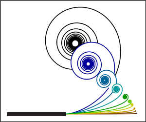
Figure 4. Examples of Type I vortex-sheet solutions. These are a family with parameter, $p$. Solutions are given for (a) $p= 0$, (b) $p=1$, (c) $p \to \infty$. For the plate motion described in § 5.1, this solution gives the sheet shape corresponding to zero initial angle of attack, $\alpha _0=0$, pivot point away from the three-quarter chord position, $d \ne 1/2$, and plate rotation dominating its translation, $m > (2 p-1)/3$, where $m$ and $p$ are the plate translation and rotation power laws, respectively. Results shown in the $\omega$-plane, which is a uniformly scaled version of the $Z$-plane; see (5.5a,b) and (5.8a,b).

For the present case, plate rotation is dominant over its translation. Indeed, our finding that (5.10) and (5.11) are independent of the composite parameter, $\hat {\beta }$, is consistent with this restriction, i.e. the geometrical structure of Type I vortex sheets do not depend on the relative strength of plate rotation-to-translation speeds; they are also independent of the rotational position, $d$.

We emphasize that Type I vortex sheets are a one-parameter family of curves and $J$ values that depend on the rotational power law, $p$. In addition to $\alpha _0=0$ studied here, it will be seen in §§ 5.3 and 5.4 that these Type I vortex-sheet solutions describe all possible starting vortices for non-zero angle of attack, $0 < \alpha _0 < {\rm \pi}/2$, with one exception (discussed end of § 5.3).

5.1.3. Type II vortex sheet

Next, we study when translational convection dominates rotational motion of the plate. This corresponds to a dominant-balance analysis between the left-hand side and the first term on the right-hand side of (5.4). Equating powers of $T$ in these terms then gives $q = 1+m$ and hence $s = p+ (m+1)/2$ via (5.3). A sub-dominant second term on the right-hand side of (5.4) requires $m < -q/2+p$ which is equivalent to $m< (2 p-1)/3$. Hence,

(5.12a,b)\begin{equation} \frac{\hat{z}_v}{a} = T^{1+m} Z(\lambda),\quad \tilde{\varGamma}\equiv \frac{\varGamma_0(T)}{U_0 a} = \mathcal{J} T^{p+({(1+m)}/{2})},\quad \text{for}\ m< \frac{2 p-1}{3},\end{equation}

where $Z(\lambda )$ is determined by solution to the linear differential equation,

(5.13)\begin{equation} (1+m) Z + \left(p +\frac{1+m}{2} \right) (1-\lambda) \frac{\textrm{d} Z}{\textrm{d}\lambda} =1,\end{equation}

subject to the initial condition in (4.2). Here, owing to the subdominant vortex-induction term in (5.4), the Kutta condition (5.1) decouples from (5.13) and can be expressed as

(5.14)\begin{equation} \mathcal{J} = \sqrt{2} {\rm \pi}\hat{\beta} \left(\int_0^1 Z^{-({1}/{2})} \,\textrm{d}\lambda \right)^{-1}. \end{equation}

Equations (5.13) and (5.14) have the exact solution

(5.15a)\begin{gather} Z(\lambda) = \frac{1}{1+m} \left( 1- (1-\lambda)^b \right), \end{gather}

(5.15b)\begin{gather}\mathcal{J} =\hat{\beta} \sqrt{\frac{2 {\rm \pi}}{1+m}} \frac{\varGamma_c\left(1+\dfrac{p }{1+m }\right)}{\varGamma_c \left(\dfrac{3}{2}+\dfrac{p}{1+m}\right)}, \end{gather}

where

(5.16)\begin{equation} b = \frac{2 (1+m)}{1 +m + 2 p}, \end{equation}

and $\varGamma _c$ is the complete gamma function (not to be confused with the circulation $\varGamma _0$). The solution for $Z(\lambda )$ in (5.15a) lies on the real axis and thus corresponds to a vortex sheet that is strictly parallel to plate (even as it rotates). We now explore how this vortex-sheet rigid body rotation arises.

Importantly, there is a weak singularity in the attached flow at the plate trailing edge which must be cancelled by finite shed circulation. Since the effect of the shed circulation and its image is still felt by the separated flow, this leads to rigid body rotation of the vortex sheet in concert with that of the plate. The overall result is that the vortex-sheet shape growth (5.15a) does not depend on the rotation parameter, $\hat {\beta }$, but the shed circulation retains dependence to order $\hat \beta$. The separation is convection dominated but (rigid body) rotational effects remain. The solution includes the limiting case of vanishing initial angle of attack, $\alpha (t) \to 0$, and plate rotation, $\hat \beta \to 0$, where the plate slices through the fluid parallel to its plane with zero shed circulation. The vortex sheet still forms and moves with the same speed, but its circulation is $O(\hat \beta )$, and thus vanishingly small as $\hat \beta \to 0$.

A (dimensional) circulation centroid can be calculated,

(5.17)\begin{equation} \langle\hat{x}\rangle = a T^{1+m} \int_0^1Z(\lambda) \,\textrm{d}\lambda = a T^{1+m} \frac{3}{3+3\,m + 2 p},\end{equation}

while the (dimensional) velocity jump at the trailing edge is

(5.18)\begin{equation} \gamma =U_0 \mathcal{J}\left(p+\frac{1+m}{2}\right) T^{p-({(1+m)}/{2})},\end{equation}

and is finite.

Type II vortex sheets are similar but not identical to point-vortex solutions obtained by Tchieu & Leonard (Reference Tchieu and Leonard2011) who use an impulse-conserving formulation. Importantly, Type II solutions exist only for zero angle of attack, $\alpha _0=0$ (the case studied here), with one exception discussed in the last paragraph of § 5.3.

5.1.4. Type III vortex sheet

The form of Type I and Type II vortex-sheet solutions above shows that, for fixed and finite $\hat \beta$, the solution changes discontinuously and remarkably as a state point in the $(m,p)$ plane crosses the line, $m = (2 p-1)/3$:

1. (a) Type I ($m >(2 p -1)/3$): a vortex-induction dominated, separated, spiral sheet exists, whose line joining the centre of roll-up to the plate trailing edge makes an angle with the positive $x$ axis greater than ${\rm \pi} /2$, i.e. the vortex core sits over the plate.

2. (b) Type II ($m <(2 p -1)/3$): a flat vortex sheet arises that separates parallel to the plate that undergoes rigid body rotation with the plate.

On the line, $m = (2 p-1)/3$, a third class of vortex sheet exists that forms an intermediate vortex-state transition (VST) between Types I and II. This is referred to as a Type III vortex sheet. With $m = (2 p-1)/3$, all terms in (5.4) then have the same power exponent of $T$ and balance, i.e. the contributions of translational convection and rotational motion of the plate balance precisely. The governing equation for Type III is nearly identical to (5.6), except it contains an extra term equal to unity on the right-hand side. Again using the change of variables in (5.8a,b), (5.4) becomes

(5.19)\begin{equation} \bar{\omega} +\frac{4 p+1}{2 (p+1)} (1-\lambda) \frac{\textrm{d} \bar{\omega}}{\textrm{d} \lambda} = \left(\frac{(1+p)\hat{\beta}^2}{3}\right)^{-({1}/{3})} -\frac{\textrm{i}}{\omega^{1/2}} \left(1 +\frac{J}{2 {\rm \pi}} I(\omega)\right), \end{equation}

while the Kutta condition (5.1) remains identical to (5.11). Here, the composite parameter, $\hat {\beta }$, cannot be scaled out, and so solutions will depend on its value. We therefore immediately see that the flow at this singular condition, $m = (2 p-1)/3$, where convection and rotation balance, produces novel separation-flow physics.

Numerical solutions to (5.11) and (5.19) are given in figures 5–7, for the example case of impulsive and constant translational plate speed, $m=0$, and a time varying angular speed with $p =1/2$. The numerical method described previously for Type I solutions is used, where a vortex discretization of $N=1,220$ is found to be sufficient for convergence (see the Appendix). Vortex sheets displayed in figures 5–7 have $15$ turns on the continuous sheet, which again is sufficient to capture the Kaden, inner asymptotic form. We show the properties of solutions in both the (stretched) $\omega$ and (unscaled) $Z$ planes. Although these are simply rescaled versions of each other, we show both because – owing to their respective divergences – the limiting solution for $\hat \beta \to \infty$ cannot be depicted using the $Z(\lambda )$-description, while the solution for $\hat \beta \to 0$ cannot be shown graphically using the $\omega (\lambda )$ function.

Figure 5. Type III vortex sheets (plate rotation balancing its translation) for zero initial angle of attack, $\alpha _0=0$, impulsive and constant translational plate speed, $m=0$, pivot point away from the three-quarter chord position, $d \ne 1/2$, with angular speed power law, $p=1/2$. Vortex sheets with visible cores (left to right): $\hat \beta \to \infty$ and $\hat \beta =1$, $0.5$, $0.3$, $0.2$. Vortex sheets with cores not visible at $\textrm {Re}\{\omega \} = 6$ (top to bottom): $\hat \beta = 0.1$, $0.05$, $0.01$. Results shown in the $\omega$-plane.

In figure 5, the vortex-sheet profiles are plotted in the $\omega$-plane for $\hat \beta \to \infty$ and ${\hat \beta = 1}$, $0.5$, $0.3$, $0.2$. The limit, $\hat \beta \to \infty$, corresponds to a Type I solution, i.e. the plate rotational motion dominates translational convection. As $\hat \beta$ decreases, the vortex core moves downstream while becoming more compact. When $\hat \beta \to 0$, the vortex core moves further downstream and approaches infinity on the real $\omega$ axis, with distance increasing as $\hat \beta ^{-2/3}$. This scaling relation follows from (5.8a,b), together with the result (to be shown subsequently in this subsection), that at the vortex-sheet free edge ($\lambda = 1$), $Z\to 1+0 i$ as $\hat \beta \to 0$. This shows the transition from rotation-dominated to convection-dominated separation. It can also be observed in figure 5, that the height of the vortex centre appears almost constant (occurring at $\textrm {Im}\{\omega \} \approx 0.75$) for solutions with $\hat \beta = 0.5$, $0.3$, $0.2$. As $\hat \beta$ decreases further, however, numerical solutions (not displayed) do show a weak but definite decrease in this height (in the $\omega$-plane), e.g. the centre of roll up when $\hat \beta = 0.001$ occurs at $\omega = 199.93 + 0.3240 i$.

Figure 6(a) shows vortex-sheet profiles in the $Z$-plane while figure 6(b) focuses on behaviour near the plate trailing edge for very small $\hat \beta$. In the $Z$-plane, the vortex-sheet extent become infinitely large as $\hat \beta \to \infty$. As $\hat \beta$ decreases, the sheet contracts in extent while the size of the rolled-up core reduces in size in comparison with the distance of the roll-up centre from the trailing edge. When $\hat \beta \to 0$, the centre approaches $Z = 1 + 0 i$ which, from (5.15a), corresponds to the flat sheet edge for a Type II vortex sheet with $m=0$. For all finite $\hat \beta$, there exists a tightly wound spiral section containing an infinite number of sheet turns. This is where vortex self-induction remains locally dominant over convection. Figure 7 shows two close-up portraits of the vortex-sheet profile in the $Z$-plane for $\hat \beta = 1$ and $0.001$. The general structure is similar. At the centre of roll up, both have the form of a Kaden spiral with small elliptical corrections of the type discussed by Moore (Reference Moore1975) and Guiraud & Zeytounian (Reference Guiraud and Zeytounian1977).

Figure 6. Type III vortex sheets, as for figure 5, but now including smaller values of $\hat \beta$ and shown in the $Z$-plane. (a) Top left to bottom right: $\hat \beta = 10$, $5$, $2$, $1$, $0.5$, $0.3$, $0.2$, $0.1$, $0.05$, $0.01$. (b) $\hat \beta = 0.1$, $0.05$, $0.01$, $0.001$, with dashed horizontal line provided for reference only.

Figure 7. Close ups of Type III vortex sheets in figure 6, for (a) $\hat \beta =1$, (b) $\hat \beta = 0.001$. For comparison, the vortex sheets are plotted on identical square domains of size, $0.3 \hat \beta \times 0.3 \hat \beta$.

Approach of Type III to the limiting Type II vortex sheet is illustrated in figure 8. This shows Cartesian coordinates of the vortex sheets, $X(\lambda ) = \textrm {Re}\{Z(\lambda )\}$ and $Y(\lambda ) = \textrm {Im}\{Z(\lambda )\}$, where $\lambda =0$ and $1$ coincide with the plate trailing edge and vortex-sheet free edge, respectively, as function of $\hat \beta$. From (5.15a), the Type II solution is simply, $Z= \lambda$, i.e. a horizontal line of finite length, for the plate control parameters studied in figures 5 and 6, i.e. $m=0$ and $p=1/2$. Approach of the Type III vortex sheet to the limiting Type II sheet, as $\hat \beta \to 0$, is clear in figure 8: $X(\lambda )$ asymptotes to the required straight line of slope one and $Y(\lambda )$ approaches zero. Notably, for any small and non-zero $\hat \beta$, there exists a small region near $\lambda = 1$ where rapid and decaying oscillations occur. This corresponds to roll-up near the vortex-sheet free edge, which approaches this free edge and vanishes in the limit of small $\hat \beta$. The small straight lines that can be seen in figure 8 near $\lambda =1$ represent the inner portion of the numerical sheet model, where its end is joined to the central point vortex.

Figure 8. Type III vortex sheets, as for figure 5, showing their Cartesian coordinates for $\hat \beta = 2$, $1$, $0.5$, $0.3$, $0.2$, $0.1$, $0.05$, $0.01$. (a) $X(\lambda ) = \textrm {Re}\{Z(\lambda )\}$ with $\hat \beta$ decreasing bottom to top, (b) $Y(\lambda ) = \textrm {Im}\{Z(\lambda )\}$ with $\hat \beta$ decreasing top to bottom. Limiting Type II solution: $Z(\lambda ) = \lambda + 0 i$.

Finally, we study the shed circulation constant, $\mathcal {J}$, defined in (4.3). For a Type II vortex sheet, with the example control parameters, $m=0$ and $p=1/2$, used in this section, (5.15b) gives

(5.20)\begin{equation} \left. \frac{\mathcal{J}}{\hat\beta} \right|_{Type\ II} = \sqrt{\frac{\rm \pi}{2}} \frac{\varGamma_c \left(\frac{3}{2}\right)}{\varGamma_c \left(2\right)} = \frac{\rm \pi}{2 \sqrt{2}} \approx 1.11072. \end{equation}

In contrast, the dependence of $\mathcal {J}$ on $\hat \beta$ for a Type III vortex sheet follows from (5.8a,b) and (5.9a,b),

(5.21)\begin{equation} \left. \frac{\mathcal{J}}{\hat\beta} \right|_{Type\ III} = \frac{1}{2} \hat\beta^{1/3} J(\hat\beta), \end{equation}

where $J(\hat \beta )$ is determined numerically. Figure 9 gives numerical results for the Type II solution in (5.21); the Type III formula, (5.20), is the dashed horizontal line. Again the approach of the Type III formula to the limiting Type II solution as $\hat \beta \to 0$ is clear. For $\hat \beta \to \infty$, $J(\hat \beta ) \to 2.3551$ and so from (5.21) we obtain

(5.22)\begin{equation} \left. \frac{\mathcal{J}}{\hat\beta} \right|_{Type\ III} \approx 1.178 \hat\beta^{1/3},\quad \hat\beta \gg 1, \end{equation}

which is shown as the dash-dot line in figure 9.

Figure 9. Shed circulation constant, $\mathcal {J}$, as a function of $\hat \beta$ for a Type III vortex sheet, with plate control parameters as specified in figure 5. Dots obtained using (5.21) for Type III vortex sheet are valid for all $\hat \beta$. Type III high $\hat \beta$ solution is dot-dashed line. For comparison, Type II solution in (5.20) is horizontal dashed line.

5.2. $\alpha _0 = 0$, $d=1/2$

This corresponds to a plate with zero initial angle of attack, $\alpha _0=0$, that is rotating about its three-quarter chord point, $d=1/2$. Here, the term in (4.4) that drives circulation growth becomes, $\tilde {Q}(T) = \beta (1+p)^{-1} T^{1+m+ p}$, plus higher-order terms in the limit of small $T$ (see (4.5b)), and we similarly expand $\cos (\alpha (t))=1 + {O}(T^{2(1+p)}) =1$, to the order required. Balancing the Kutta condition, (4.6), then gives

(5.23)\begin{equation} s=\frac{q}{2}+m+p+1, \end{equation}

and (4.6) becomes

(5.24)\begin{equation} \frac{\mathcal{J}}{4 {\rm \pi}} \int^1_0 \left( \frac{1}{Z^{1/2} } +\frac{1}{\bar{Z}^{1/2}} \right) \textrm{d}\lambda = \frac{1}{2^{1/2}} \frac{\beta}{1+p}. \end{equation}

Substituting (5.23) into (4.4) gives

(5.25)\begin{align} & T^{q-1} \left(q \bar{Z} + \left[\frac{q}{2} +1+m +p\right](1-\lambda) \frac{\textrm{d} \bar{Z}}{\textrm{d} \lambda}\right)\nonumber\\ &= T^m-T^{-({q}/{2})+1+m+p} \frac{\textrm{i}}{Z^{1/2}} \left(\frac{1}{2^{1/2}} \frac{\beta}{1+p} + \frac{\mathcal{J}}{4 {\rm \pi}} I(Z) \right). \end{align}

Again, there are three flow types. The first arises from a dominant balance between the left-hand side and the second term on the right-hand side of (5.25), i.e. a plate rotation-dominated flow. This gives $q = 2 (2+m+p)/3$ and $s = (5+4 m+4 p)/3$ with

(5.26a,b)\begin{equation} \frac{\hat{z}_v}{a} = T^{({2}/{3}) (2+m+p)} Z(\lambda),\quad \tilde{\varGamma} = \mathcal{J} T^{({1}/{3})(5+4 m+4 p)},\quad \text{for}\ m> 1+2 p, \end{equation}

where $Z(\lambda )$ and the shed circulation constant, $\mathcal {J}$, are determined from the solution of an integro-differential equation similar to (5.1) and (5.6).

A plate translation-dominated flow is obtained by performing a dominant balance between the left-hand side and the first term on the right-hand side of (5.25), giving $q = 1+ m$ and $s = 3 (1+m)/2+p$, with

(5.27a,b)\begin{equation} \frac{\hat{z}_v}{a} = T^{1+m} Z(\lambda),\quad \tilde{\varGamma} = \mathcal{J} T^{({3}/{2}) (1+m)+p},\quad \text{for}\ m< 1+2 p, \end{equation}

where $Z(\lambda )$ and $\mathcal {J}$ are obtained from solution of a linear system similar to (5.13) and (5.14), giving a Type II vortex sheet. The balance, $m = 1+2 p$, gives a Type III vortex sheet similar to that described earlier but with different power laws and constants; details are left to the reader.

5.3. $\alpha _0 \ne 0$, $d \ne 1/2$

We now consider a plate with non-zero initial angle of attack, $\alpha _0\ne 0$, that is rotating away from its three-quarter chord point, $d\ne 1/2$. The Kutta condition, (4.6), to leading order in $T$ is

(5.28)\begin{align} \frac{\mathcal{J}}{4 {\rm \pi}} T^{s-({q}/{2})} \int^1_0 \left(\frac{1}{Z^{1/2} } + \frac{1}{\bar{Z}^{1/2}}\right) \textrm{d}\lambda = \frac{1}{2^{1/2}}\left( T^p \hat\beta + T^m \left[\sin\alpha_0 +T^{1+p}\frac{\beta}{1+p} \cos\alpha_0 \right]\right). \end{align}

We again consider three cases:

1. (a) $p<m$: Suppose the plate rotation power law is less than that for plate translation, i.e. $p<m$, and recall that $m, p\ge 0$. Then from (5.28), dominant balance gives $s = q/2 +p$. The $T$ power laws of the second and third terms in (4.4) are both $-q/2 +p$. A dominant balance between the left-hand side of (4.4) and these two terms now gives $q=2 (p+1)/3$ and $s = (4 p+1)/3$. Thus, the $T^m$ term in $\tilde {Q}$ in (4.5b) is subdominant. The first term on the right-hand side of (4.4) again is always subdominant for $m>0$. This case is identical to (5.6) and (5.7) (zero initial angle of attack) and gives a Type I vortex sheet, i.e. the start-up motion is rotation dominated.

2. (b) $p>m$: Now consider the opposite case. From (5.28), the first term on its right-hand side is subdominant, giving $s = q/2 +m$. The $T$ power-laws of the second and third terms on the right-hand side of (4.4) are both $-q/2 +m$. A dominant balance between the left-hand side of (4.4) and these two terms then gives $q=2 (m+1)/3$ and $s = (4 m+1)/3$; the first term on its right-hand side is always subdominant for $m>0$. This case is identical to (5.6) and (5.7) with $p$ and $\hat \beta$ replaced by $m$ and $\sin \alpha _0$, respectively. This gives a Type I vortex sheet, but one that is convection dominated due to non-zero angle of attack (rather than rotation dominated). This is equivalent to a start-up flow with no plate rotation, $\hat \beta =0$, and non-zero angle of attack, $\alpha _0 >0$ (Pullin Reference Pullin1978).

3. (c) $p=m$: This case is delicate, and we first consider $\hat \beta + \sin \alpha _0 \ne 0$. The $T^{1+p}$ term on the right-hand side of (5.28) is subdominant. Both surviving terms on the right-hand side of (5.28) balance while the term proportional to $T^m$ in (4.4) remains subdominant. This is the same as $p<m$ in case (a) above with $\hat \beta$ replaced by $\hat \beta + \sin \alpha _0$, i.e. a Type I vortex sheet that arises from a balance between convection and rotation. As a parameter point in $(m,p)$ space crosses the line $m=p$, the $T$ power laws and the Type I vortex sheet solution are continuous. However, $Z(\lambda )$ will always be twice discontinuous and the dominant physics will change from rotation-dominated (case (a)) to rotation-convection balanced (this case) to convection dominated (case (b)).

Next, we study $p=m$ but now with $\hat \beta + \sin \alpha _0 = 0$. Here, the right-hand side of (5.28) and $\tilde {Q}$ in (4.5b) are proportional to $T^{1+2 p}$, to leading order. Equation (5.28) then gives, $s= q/2+2 p+1$. Now consider a dominant balance between the left-hand side and the second and third terms of (4.4). A short calculation gives

(5.29)\begin{equation} q=\tfrac{4}{3} (1+p), \end{equation}

and $s = (5+8 p)/3$. For the convective (first) term on the right-hand side of (4.4) to be subdominant relative to its left-hand side, we require $p>q-1$. Substituting (5.29) into this inequality then gives $p < -1$, which violates the overriding constraint, $p \ge 0$, in (2.10a,b). Hence, these solutions do not exist. The other possibility is a balance between the left-hand side and the convective term on the right-hand side of (4.4). This gives $q=1+p$ and $s = (3+5 p)/2$, leading to a Type II convective-dominated starting vortex. This is the exceptional case where a Type II solution exists for $\alpha _0\ne 0$.

5.4. $\alpha _0 \ne 0$, $d=1/2$

Finally, we study $d=1/2$ where the rotation pivot is at the three-quarter chord point, with non-zero initial angle of attack, $\alpha _0 \ne 0$. Here, the second terms in the arguments of the $\cos \alpha (t)$ and $\sin \alpha (t)$ in (4.4) and (4.5b), respectively, can be neglected for $T\ll 1$ while the term, $T^p \beta (1/2-d)$, in (4.5b) is zero. Equations (4.4) and (4.5b) then become

(5.30a)\begin{align} T^{q-1} \left(q \bar{Z} + s (1-\lambda) \frac{\textrm{d} \bar{Z}}{\textrm{d} \lambda}\right) &= T^m \cos\alpha_0\nonumber\\ &\quad -T^{-({q}/{2})+m}\frac{\textrm{i}}{Z^{1/2}} \left(\frac{1}{2^{1/2}} \sin\alpha_0 +\frac{\mathcal{J}}{4 {\rm \pi}} I(Z)\right), \end{align}

(5.30b)\begin{equation} \frac{\mathcal{J}}{4 {\rm \pi}} T^{s-({q}/{2})} \int^1_0 \left(\frac{1}{Z^{1/2}} + \frac{1}{\bar{Z}^{1/2}} \right) \textrm{d}\lambda = \frac{1}{2^{1/2}} T^m \sin\alpha_0. \end{equation}

From (5.30b), finite shed circulation requires $s= q/2+m$. We seek a dominant balance between the left-hand side and the (rotational) second and third terms on the right-hand side of (5.30a), which gives $q=2 (1+m)/3$ and $s = (4 m+1)/3$. A subdominant first term on the right-hand side of (5.30a) requires $m> q-1$, which upon substitution of the preceding expression for $q$, gives $m>-1$. This inequality is always satisfied since $m \ge 0$; see (2.10a,b). The resulting equations are identical to (5.5a,b) and (5.6) with $p$ and $\hat \beta$ replaced by $m$ and $\sin \alpha _0$, respectively. This is again a Type I vortex sheet, but is convection dominated due to non-zero initial angle of attack. There exists no solution with a dominant balance between the left-hand side and (convective) first term on the right-hand side of (5.30a). This would require $q=1+m$ while a subdominant second-third term on the right-hand side needs $q < 0$. These two expressions for $q$ imply that $m < -2$ which is not allowed, notwithstanding that $q \ge 0$ is required; see (4.1a,b).

5.5. Summary of vortex types

Table 1 summarizes the results of the analyses in §§ 5.1–5.4, the key points of which are:

1. (a) Type I vortex sheets appear in each of the four distinct plate motions, for certain parameter ranges.

2. (b) Type II vortex sheets are restricted to zero initial angle of attack, $\alpha _0 =0$, over certain parts of the $(m,p)$ plane, and also to $\alpha _0 \ne 0$ under the condition that both, $m=p$, and, $\hat \beta + \sin \alpha _0 = 0$.

3. (c) Type III sheets appear only for zero initial angle of attack, $\alpha _0 =0$, along the lines (i) $m= 1+2 p$ for plate rotation about its three-quarter chord position, $d =1/2$, and (ii) $m= (2 p-1)/3$ for $d \ne 1/2$.

The right-hand column of table 1 indicates the dominant physics that control the starting vortex for each of the eleven flow regimes shown. Type I vortex sheets appear for both strict rotation and convection-dominated flows, and in one case for a combination of rotation and convection. Type II sheets occur only for convection dominated starting vortices. Because Type III vortex sheets describe a transition regime, these are always controlled by a mix of rotation and convection.

5.6. Vanishing plate rotation and degenerate vortex sheets

The present theory assumes the plate always rotates, i.e. $\varOmega _0 > 0$ and hence $\beta > 0$. It is also of interest to study the limit of vanishing plate rotation, i.e. $\alpha (t) = \alpha _0 = \text {constant}$, because this can align with problems of practical interest. For example, the widely studied start-up of a flat plate at constant translational speed and fixed non-zero angle of attack (Prandtl Reference Prandtl1924). Interestingly, some starting vortices in table 1 present singular solutions for vanishing plate rotation, i.e. the limit $\beta \to 0^+$ differs from $\beta = 0$, while others are continuous. Thus, care must be taken when applying such singular configurations in a practical setting, because even a small amount of rotation can potentially change the resulting shed (primitive) vortex.

We provide two examples for fixed non-zero angle of attack, $\alpha (t) = \alpha _0 > 0$:

1. (a) Consider the above-mentioned flow of a plate moving with impulsive and constant translational speed, $m=0$ (Prandtl Reference Prandtl1924). Regardless of the plate rotation power law, $p\ge 0$, table 1 shows that a Type I vortex sheet arises with vortex power law, $q = 2/3$, as the plate rotation speeds approaches zero, i.e. $\beta \to 0^+$. This vortex power law of 2/3 is identical to the result for identically zero rotation; see page 414 of Pullin (Reference Pullin1978), who studied a semi-infinite plate, the results of which are applicable here because the leading edge of a finite plate does not affect its primitive trailing-edge vortex; see § 1. That is, the solution is continuous in the limit, $\beta \to 0^+$.

2. (b) Next, we study the related problem of a plate undergoing constant acceleration, ${m=1}$, with the rotation pivot point away from the three-quarter chord position, $d \ne 1/2$. If the plate rotation power law, $p < m\ (=1)$, table 1 shows that a Type I (rotation dominated) vortex sheet emerges with a vortex power-law of $q=(2/3)(1+p)$, as $\beta \to 0^+$. Thus, even though the plate angular speed approaches zero, the vortex dynamics is still intimately controlled by plate rotation. In contrast, if $p > m\ (=1)$, a Type I (convection dominated) vortex sheet emerges with a vortex power law of $q = 4/3$, i.e. the vortex dynamics is independent of plate rotation; the same vortex power law holds for $p = m\ (= 1)$. Consequently, vortex dynamics from this plate motion exhibits singular behaviour: (i) the limit of infinitesimal plate rotation, $\beta \to 0^+$, depends on the plate rotation power-law, $p$, while (ii) identically zero plate rotation, $\beta = 0$, is by definition independent of $p$.

This degeneracy in these (inviscid) vortex dynamics is likely resolved in a practical setting through the influence of viscosity. The same holds for any degeneracy that may be encountered for vanishing plate translation. These remain open questions.

7.1. Type I vortex sheet

We first study Type I vortex sheets that are rotation dominated. A similar analysis for other Type I solutions is straightforward. Near the leading edge of the flat plate, the outer inviscid complex potential follows from (2.8),

(7.1)\begin{equation} W(\hat{z},t) =-\textrm{i}At^p \hat{z}^{{1}/{2}} + \cdots, \end{equation}

where $A = D(a/2)^{{3}/{2}} \varOmega _0(U_0/a)^p$ and $D= 1/2-d$. The dimensions of $A$ are length$^{{3}/{2}}\times \textrm {time}^{-(1+p)}$.

Consider some point-wise quantity that characterizes the vortex growth, such as the (dimensional) centre of a vorticity distribution, $\hat {z}_c$. Because vorticity takes finite time to diffuse from the plate, the outer flow remains essentially inviscid during the early-time viscous vortex growth. It is then assumed that for a viscous flow at sufficiently small times, where the starting vortex remains close to the leading edge, the dependence of $\hat {z}_c$ on the plate and flow parameters takes the functional form

(7.2)\begin{equation} \hat{z}_c = \hat{z}_c(A,t,\nu \,|\, p), \end{equation}

where $\nu$ is the kinematic viscosity of the fluid. That is, the vorticity distribution centre depends on the rotational power law, $p$, but not the translational power law, $m$; see (2.10a,b). Dimensional analysis then gives

(7.3)\begin{equation} \frac{\hat{z}_c}{A^{{2}/{3}}t^{({2}/{3})(1+p) }} = F(Re_t \, | \, p),\end{equation}

where $F(Re_t \, | \, p)$ is a dimensionless function (to be determined), and

(7.4)\begin{equation} Re_t = \frac{A^{{4}/{3}}t^{({1}/{3})(1+4p)}}{\nu}, \end{equation}

is a time-dependent Reynolds number.

For the shed circulation, $\varGamma _s$, at time, $t$, a similar analysis gives

(7.5)\begin{equation} \varGamma_s = A^{{4}/{3}}t^{({1}/{3})(1+4p)} G(Re_t \, | \, p),\end{equation}

where $G(Re_t \,|\, p)$ is another dimensionless function. From (4.1a,b), the vorticity distribution centre is given by $\hat {z}_c = \hat {z}_v(\lambda =1,t)$, corresponding to the centre of the inviscid vortex roll up. Equations (5.5a,b) and (5.9a,b) then give

(7.6a)\begin{gather} F(Re_t \, | \, p) = \left(\frac{3}{1+p}\right)^{{2}/{3}}\omega(\lambda=1,p), \end{gather}

(7.6b)\begin{gather}G(Re_t \, | \, p) = 4J(p)\left(\frac{3}{1+p}\right)^{{1}/{3}}, \end{gather}

which are both independent of $Re_t$, where $J(p)$ is defined in (5.8a,b).

For the rotation-dominated Type I vortex considered here, $Re_t$ is related to the plate Reynolds number, $Re_c \equiv 2a U_0/\nu$, by

(7.7)\begin{equation} Re_t = Re_c\tfrac{1}{8}\hat{\beta}^{{4}/{3}} T^{({1}/{3})(1+4p)}.\end{equation}

Two limits are of practical interest:

1. (a) $Re_c\to \infty$ at fixed and finite $T$. Equation (7.7) then gives $Re_t\to \infty$, i.e. both Reynolds numbers are infinite. A reasonable but unproven hypothesis is that this limit would produce a turbulent starting vortex whose structure may or may not be related to the present inviscid similarity solution.

2. (b) $Re_c\to \infty$ and $T\to 0$ such that $Re_t$ is fixed and moderately large. Importantly, inviscid theory finds support from experiment and viscous simulation for moderately large $Re_c$ and $Re_t$. For example, figure 4(e) of Pullin & Perry (Reference Pullin and Perry1980) shows reasonable agreement between experiment and the inviscid theory (for $z_c$) for wedges and thin plates with $Re_t\sim 10^3\text {--}10^6$. Similarly, Xu et al. (Reference Xu, Nitsche and Krasny2017) report good agreement between viscous and inviscid solutions for the location, size and shape of the vorticity spiral vortex cores, and also for the shed circulation as a function of time, for $Re_c =250\text {--}2000$. These previous studies suggest that similar agreement may be found for the present problem in this limit of very small convective time, $T \ll 1$, at moderately large $Re_t$.

7.2. Type II vortex sheet

For a Type II, convection-dominated vortex sheet, (7.2) is replaced by

(7.8)\begin{equation} \hat{z}_e = \hat{z}_e (a,U_0,t,\nu \, | \, p,m), \end{equation}

where $\hat {z}_e$ refers to the free end of the sheet. That is, the solution depends on both the translational and rotational power laws, $m$ and $p$, respectively. Dimensional analysis then gives

(7.9a,b)\begin{equation} \frac{\hat{z}_e} {a} = H(T,Re_t \, | \, p,m),\quad \frac{\varGamma_s} {U_0\,a} =M(T,Re_t \, | \, p,m),\end{equation}

where $H(T,Re_t \, | \, p,m)$ and $M(T,Re_t \, | \, p,m)$ are dimensionless functions, and

(7.10)\begin{equation} Re_t = Re_c \frac{T}{2}. \end{equation}

From § 5.1.3, we then find

(7.11a,b)\begin{equation} H(T,Re_t \, | \, p,m) = \frac{1}{1+m}T^{1+m},\quad M(T,Re_t \, | \, p,m) = \mathcal{J}\, T^{p+({(1+m)}/{2})},\end{equation}

which are again independent of $Re_t$. A large Reynolds number limit analysis can be performed, as for the Type I vortex sheet; this is left to the reader.

Experiments or viscous-resolved computational simulations that could distinguish the formation Type I or Type II structures in the $(m-p)$ plane for moderate $Re_t$ would seem feasible.