


1. Introduction
Flow unsteadiness is a major factor characterising both wind and tidal-stream energy production. For example, dealing with wind resource variability remains one of the biggest challenges in wind energy research, as the lack of long-term predictions can affect production, storage and distribution of energy (van Kuik et al. Reference van Kuik, Peinke, Nijssen, Lekou, Mann, Sørensen, Ferreira, van Wingerden, Schlipf and Gebraad2016; Veers et al. Reference Veers, Dykes, Lantz, Barth, Bottasso, Carlson, Clifton, Green, Green and Holttinen2019). On the other hand, large-scale variations in tidal channels caused by ebb and flood are highly predictable. Yet, site-specific and regional-scale flow phenomena can introduce flow velocity variations beyond the tidal cycle and increase flow unsteadiness upstream of tidal turbines (Adcock, Drapper & Nishino Reference Adcock, Drapper and Nishino2015). At rotor scale, flow unsteadiness is characterised by small-scale, turbulence-driven fluctuations. The level of turbulence intensity within tidal channels has been reported to be as high as 15–20 % (Grant, Stewart & Moilliet Reference Grant, Stewart and Moilliet1962; Heathershaw Reference Heathershaw1979; Osalusi, Side & Harris Reference Osalusi, Side and Harris2009a,Reference Osalusi, Side and Harrisb), while analogous wind energy site measurements have reported values closer to 8–12 % (Hansen et al. Reference Hansen, Barthelmie, Jensen and Sommer2012; Milan, Wächter & Peinke Reference Milan, Wächter and Peinke2013). To understand the effect of turbulence on wind or tidal-stream power output variability, numerous studies have attempted to quantify the impact of upstream turbulence on a single horizontal-axis turbine (Chamorro et al. Reference Chamorro, Hill, Morton, Ellis, Arndt and Sotiropoulos2013, Reference Chamorro, Lee, Olsen, Milliren, Marr, Arndt and Sotiropoulos2015; Tobin, Zhu & Chamorro Reference Tobin, Zhu and Chamorro2015; Payne et al. Reference Payne, Stallard, Martinez and Bruce2018) or turbine arrays (e.g. wind farms) (Stevens & Meneveau Reference Stevens and Meneveau2014; Bossuyt et al. Reference Bossuyt, Howland, Meneveau and Meyers2016; Stevens, Gayme & Meneveau Reference Stevens, Gayme and Meneveau2016; Bandi Reference Bandi2017; Bossuyt, Meneveau & Meyers Reference Bossuyt, Meneveau and Meyers2017; Tobin & Chamorro Reference Tobin and Chamorro2018). Moreover, indirect measurements from the electrical power output for more than one wind farm (Apt Reference Apt2007; Katzenstein, Fertig & Apt Reference Katzenstein, Fertig and Apt2010; Vigueras-Rodríguez et al. Reference Vigueras-Rodríguez, Sørensen, Cutululis, Viedma and Donovan2010) have also been obtained and studied. These works have shown that both the individual and aggregate array power output are strongly modulated by small-scale turbulence and larger coherent structures. In particular, the time scales and magnitude of power output fluctuations that can both be compactly described by the respective power spectra density functions of the power fluctuations (power spectra) have shown to exhibit a behaviour that deviates from that of the onset velocity spectra.
Studies of a single horizontal-axis turbine (HAT) interacting with onset turbulence have shown that the rotor behaves as a low-pass filter by ignoring the small-scale fluctuations and responding only to the larger coherent structures (Chamorro et al. Reference Chamorro, Lee, Olsen, Milliren, Marr, Arndt and Sotiropoulos2015; Tobin et al. Reference Tobin, Zhu and Chamorro2015; Anvari et al. Reference Anvari, Lohmann, Wächter, Milan, Lorenz, Heinemann, Tabar, Reza and Peinke2016). To this end, Tobin et al. (Reference Tobin, Zhu and Chamorro2015) proposed a power law with a slope of  $-11/3$ to be more appropriate over the inertial sub-range, where the incoming velocity fluctuates according to the well-known
  $-5/3$ power law of isotropic turbulence (Kolmogorov Reference Kolmogorov1941; von Kármán Reference von Kármán1948). Additionally, they attributed the resulting
  $-2$ slope difference between the velocity and power fluctuations to the rotational motion of the blades, a behaviour that was later confirmed by the spectral behaviour of a different rotating structure (rotating plate) (Jin, Ji & Chamorro Reference Jin, Ji and Chamorro2016). Other studies have also reported an excess of energy in the narrow band around the blade-passing frequency (BPF)
  $f_b=N_b \varOmega /(2{\rm \pi} )$, where
  $\varOmega$ is the rotor angular speed and
  $N_b$ the number of blades (Chamorro et al. Reference Chamorro, Hill, Morton, Ellis, Arndt and Sotiropoulos2013; Payne et al. Reference Payne, Stallard, Martinez and Bruce2018). On the other hand, power fluctuations aggregated over arrays of turbines were found to exhibit a behaviour much closer to that of the velocity fluctuations. Apt (Reference Apt2007) considered a small array of six turbines and found a power law slope of
  $-5/3$ over the low-frequency regime and a
  $-7/2$ scaling over the higher frequencies of the inertial sub-range. For larger turbine clusters however, Stevens & Meneveau (Reference Stevens and Meneveau2014) and Bossuyt et al. (Reference Bossuyt, Howland, Meneveau and Meyers2016) found that the power law of
  $-5/3$ is sustained over the inertial sub-range whereas for the same frequency range, Liu et al. (Reference Liu, Jin, Tobin and Chamorro2017) and Bossuyt et al. (Reference Bossuyt, Meneveau and Meyers2017) found a power-law behaviour of
  $f^{-11/3}$, and between
  $f^{-5/3}$ and
  $f^{-2}$, respectively. Even more interesting, the same studies found that the aggregate power spectra exhibit characteristic peaks at integer multiples of the advective frequency
  $f_a=2 {\rm \pi}/T_a$, where
  $T_a$ corresponds to the mean velocity-driven travel time between two adjacent in-line turbines. To explain the existence of these peaks, first Bossuyt et al. (Reference Bossuyt, Meneveau and Meyers2017) and later Tobin & Chamorro (Reference Tobin and Chamorro2018) and Tobin et al. (Reference Tobin, Lavely, Schmitz and Chamorro2019) used the random-sweeping hypothesis of Kraichnan (Reference Kraichnan1964) and Tennekes (Reference Tennekes1975) following previous studies that utilised the same theory to obtained spatio-temporal spectral correlations in the logarithmic layer of wall turbulence (Wilczek, Stevens & Meneveau Reference Wilczek, Stevens and Meneveau2015a,Reference Wilczek, Stevens and Meneveaub).
In this study we present a novel semi-analytical model for the power spectra of a single HAT. In particular, we consider both the turbulence immediately upstream of the rotor and the forces that it induces on the rotor. First, in the case of the inflow velocity field, the turbulence is distorted, as was recently shown by Graham (Reference Graham2017), Milne & Graham (Reference Milne and Graham2019) and Mann et al. (Reference Mann, Peña, Troldborg and Andersen2018). This is an effect of flow being blocked and distorted by the projected thrust force, thereby leading to a pronounced decrease in the spectral amplitude of the approaching velocity over the low-frequency regime. Second, the effect of low-pass filtering that is observed in the inertial sub-range as well as the energy amplification around the blade-passing frequency are both due to rotational effects and will be calculated using the rotationally sampled spectra (RSS) technique (Connell Reference Connell1982). To validate the proposed model, a series of experiments conducted in the water flume in the Institut Français de Recherche pour l'Exploitation de la MER (IFREMER) at Boulogne-sur-Mer, France are presented. The experiments consider synchronous measurements of the approaching velocity field at different locations upstream of the rotor and the respective rotor turbine's generated torque.
The remaining sections of this paper are organised as follows. Section 2 introduces the underlying theory of turbulence distortion, analytical derivation of the linearised relationship between the velocity and power fluctuations and the application of RSS analysis to derive a rotor velocity cross-correlation function and the power spectral density function of the power fluctuations for a three-bladed turbine. In § 3 we present the experimental set-up as well as the methods used to obtain synchronised turbulence/turbine measurements are presented. A parametric study for our semi-analytical model is presented in § 4 while an extensive comparison between the experimental data and the model predictions is provided in § 5. Finally, a brief summary and discussion of our main findings as well as the limitations of our model are presented in § 6.
2. Problem definition
We consider a spatially uniform velocity field,  $\boldsymbol {u}_\infty =(u_{1\infty },u_{2\infty },u_{3\infty })$, approaching a horizontal-axis turbine with diameter
  $D$ (see figure 1). By applying Reynolds decomposition to the uniform velocity field, we obtain a mean (
 $U_{i\infty }$) and a fluctuating part,
  $u_{i\infty }^\prime$. As the incoming flow approaches the rotor, the fluctuating velocity field gets distorted, thanks to the combined effects of the rotor's blockage and projected mean strain (Graham Reference Graham2017; Milne & Graham Reference Milne and Graham2019), thus altering the incoming mean flow and turbulence characteristics that eventually reach the rotor. The distorted velocity field at some location,
  $\boldsymbol {x}=(x_1,x_2,x_3)$, upstream the rotor is denoted by
  $\boldsymbol {u}=(u_1,u_2,u_3)$. The interaction of the distorted velocity field with the rotor system thereafter leads to time-varying power generation that can be accurately calculated through the rotor's torque,
  $Q(t)$, so that
  $P(t)=Q(t) \varOmega$. Here, we have assumed that the turbine rotates with a constant angular velocity,
  $\varOmega$.In the absence of time-dependent torque measurements, however, the time-varying power output of a single turbine can be calculated based on the inflow velocity, as the two are inherently related. A commonly used approach to calculate the power fluctuations from the approaching velocity field is to utilise the steady-state, disk-averaged expression,
 \begin{equation} P(t)=\tfrac{1}{2} \rho C_P A u_{1\infty}^3(t), \end{equation}
where  $\rho$ is the fluid density,
  $C_P$ is the mean power coefficient and
  $A={\rm \pi} R^2$ is the rotor area. Such an approach has been successfully employed by Bossuyt et al. (Reference Bossuyt, Howland, Meneveau and Meyers2016, Reference Bossuyt, Meneveau and Meyers2017) for the spatially averaged power fluctuations over large wind farms. Because (2.1) is derived from steady-state analysis and represents disk-averaged quantities, it is not expected to be able to capture small-scale fluctuations and its true effect on the power output. Equation (2.1) can be more suitably used for power output calculations of a rotor interacting with larger coherent structures (typically with length scales greater than one rotor diameter). Nonetheless, the turbine power time series from these two approaches may be used to calculate the power spectra via the Fourier transform of the signal's autocovariance function
  $\langle P(t) P(t+\tau ) \rangle$ as
 \begin{equation} S_P(\,f)= \int_{-\infty}^{\infty} \langle P(t) P(t+\tau)\rangle \exp({-\textrm{i} 2 {\rm \pi}f \tau})\, \mathrm{d} \tau, \end{equation}
where  $\langle * \rangle$ denotes the expected value and
  $f$ the frequency in hertz (Hz). Using experimental data from this study for a single, optimally operated red (based on the rotor's tip-speed ratio
  $\lambda = \varOmega D/ 2 U_{1\infty }$), three-bladed, horizontal-axis turbine, we find large discrepancies in both the estimated power fluctuations and power spectra between the ‘disk-averaged’ and torque-based estimations. The ‘disk-averaged’ calculations are done using the turbine-synchronous instantaneous upstream velocity,
  $u(t)$ at
  $x_1=-D$ (one diameter upstream of the rotor), and then shifted in time according to Taylor's frozen turbulence hypothesis (
 ${\rm \Delta} x=-U_{1\infty }{\rm \Delta} t)$. On the other hand, the torque-based calculation uses the time-averaged but nearly constant rotational speed,
  $\varOmega$, and the experimentally measured instantaneous turbine torque. The comparison of these two methods reveals discrepancies between the two approaches, which are highlighted in figure 2. The two approaches appear to differ significantly over short time scales, with the ‘disk-averaged’ formula failing to reproduce both the spectral filtering and spectral amplification over the inertial and BPF regimes, respectively. In fact, the two approaches agree well only for the larger time scales (low-frequency regime). To address these discrepancies, we employ standard analytical tools from turbulence theory and aerodynamics and propose a novel semi-analytical model, which accurately captures the spectral behaviour of the power fluctuations and reveals the underlying mechanisms that affect it. For our analysis, we shall assume that the rotor is always aligned with the mean incoming flow,
  $U_{2\infty }=U_{3\infty }=0$, as well as that the velocity fluctuations,
  $u^\prime _j=u_j-U_j$, can be best described by isotropic and homogeneous turbulence in the far-upstream velocity fields. Finally, any aeroelastic effects of the rotor blades and other supporting structures will be neglected.

Figure 1. Schematic representation of upstream turbulence approaching a horizontal-axis turbine and the transformation process between velocity and power fluctuations. Figure adapted from Tobin et al. (Reference Tobin, Zhu and Chamorro2015).

Figure 2. Comparison between measured power fluctuations and estimated ones based on the mean power formula. (a) Time series of the power fluctuations with a zoomed-in plot showing the large discrepancies over short time scales. (b) Power spectral density functions of power fluctuations with annotations for the respective scaling law slopes and spectral content over the BPF.
2.1. Distortion of the approaching turbulence upstream of the rotor
As free-stream turbulence approaches the rotor, it becomes distorted as it gets subjected to the mean velocity strain (vorticity distortion) and the rotor's blockage effect. In a recent study, Graham (Reference Graham2017) applied the rapid distortion theory of Batchelor & Proudman (Reference Batchelor and Proudman1954) to a general length-scale turbulence approaching the rotor and calculated the distorted spectra of the streamwise velocity. Their study concluded that by considering only the turbulent vorticity distortion effect and for a small turbulence integral length scale to rotor diameter ratio  $L_{1\infty }/D$, the magnitude of the large-scale's fluctuations can be amplified. A subsequent analysis by Milne & Graham (Reference Milne and Graham2019), however, considered both effects (blockage and vorticity distortion) by decomposing the streamwise fluctuations into a rotational and irrotational velocity field (Helmholtz decomposition). They showed that in turbulent flows characterised by larger integral length scales, the blockage effect dominates, resulting in a substantial attenuation of the low-frequency components. Here, we argue that turbulence-to-rotor interactions are most commonly characterised by large integral length scales, ignore vorticity distortion and make all of our consequent analysis by only considering the rotor's blockage distortion effect. To that extent, we postulate that the root mean square (r.m.s.) of the upstream velocity fluctuations,
  $\sqrt {\overline {u^{\prime 2}_{1}}}$, can be adequately calculated by analogy to the upstream mean velocity field,
  $U_1=(1-af_s(x_1))U_{1\infty }$,
 \begin{equation} \sqrt{\overline{u^{\prime 2}_{1}}}= \sqrt{\overline{u^{\prime 2}_{1\infty}}} \left( 1 -a f_s(x_1)\right), \end{equation}
where  $f_s(x_1)$ represents a dimensionless mean perturbation velocity function at a distance
  $x_1$ upstream of the rotor, and
  $a$ the axial induction factor. This assumes that the steady flow theory can be applied to the unsteady flow components in turbulence for low frequencies similar to Mann et al. (Reference Mann, Peña, Troldborg and Andersen2018). To approximate
  $f_s$, we shall make use of the actuator disk solution of Conway (Reference Conway1995),
 \begin{equation} U_1(x_1)= U_{1\infty}\left[1-a\left(1+\frac{x_1/D}{\sqrt{(x_1/D)^2+1/4}} \right) \right], \quad x_1 <0 \end{equation}
and calculate the axial induction factor through the rotor's thrust coefficient,  $C_T$,
  $a=1/2(1-\sqrt {1-C_T})$, while
 \begin{equation} f_s(x_1)=1+\frac{x_1/D}{\sqrt{(x_1/D)^2+1/4}}, \quad x_1<0. \end{equation}
Furthermore, we may also define a distortion factor,  $\gamma$, as
 \begin{equation} \gamma = \sqrt{\frac{\overline{u^{\prime 2}_{1}}}{\overline{u^{\prime 2}_{1 \infty}}}} = \frac{U_1}{U_{1 \infty}}, \end{equation}
and thereupon the one-dimensional, streamwise, autocorrelation function,  $R_{11}=\langle u^\prime _1(x_1, t+\tau ) u^\prime _1(x_1 , t) \rangle$, by considering both the local distortion factor and the shifted coordinates,
 \begin{equation} \langle u_1^\prime(x_1, t) u_1^\prime(x_1, t+\tau) \rangle = \gamma^2 \langle u_{1\infty}^\prime(x_1-\chi(\tau), t) u_{1\infty}^\prime(x_1-\chi(\tau), t+\tau) \rangle, \end{equation}
where  $\chi (\tau )$ is the travel distance (spatial shift) of turbulence by the local mean velocity. The spatial shift function,
  $\chi (\tau )$, obeys the following equation:
 \begin{equation} \frac{\mathrm{d} \chi(\tau) }{\mathrm{d} \tau}+a U_{1\infty}(\chi)\frac{\chi/D}{\sqrt{(\chi/D)^2+1/4}} =(1-a)U_{1\infty} \end{equation}
which is a first-order nonlinear ordinary differential equation (ODE) that we solve here numerically using the explicit fourth-order Runge–Kutta (RK4) method. The solution is shown in figure 3 for different axial induction factor values:  $a=0.1$, 0.3 and 0.4 together with the undistorted solution,
  $a=0$. From the autocorrelation function we may also obtain the velocity spectra through a Fourier transform so that
 \begin{equation} S_{11}(\,f)= \gamma^2 S_{11\infty}(\,f), \end{equation}
a relationship between the distorted,  $S_{11}(\,f)$, and undistorted spectra,
  $S_{11\infty }(\,f)$, which agrees well with Mann et al. (Reference Mann, Peña, Troldborg and Andersen2018) for below-rated conditions (
 $\mathrm {d}a/\mathrm {d}U_{1\infty }=0$). Finally, for all of our subsequent calculations of both the far-upstream undistorted and near-rotor distorted velocity spectra, we shall use the von Kármán spectrum model,
 \begin{equation} S_{11}(\,f)= \gamma^2 \frac{4\overline{u^{\prime 2}_{1\infty}} L_{1\infty}/U_{1\infty} }{[1+70.8(\,f \kern0.5pt L_{1\infty}/U_{1\infty})^2]^{5/6}}. \end{equation}
Note that, for  $x_1 \rightarrow -\infty$,
  $\gamma \rightarrow 1$ and, thus, the far-upstream undistorted spectrum is restored.

Figure 3. Numerical solution of the velocity fluctuations spatial shift distance,  $\chi$, by the mean flow,
  $U_{1}$, as a function of time lag,
  $\tau$. Assuming a constant upstream velocity,
  $U_{1\infty }$, the solution yields the standard,
  $\chi (\tau )=-U_{1\infty }\tau$. Both the spatial shift,
  $\chi$, and time lag,
  $\tau$, are presented in a non-dimensionalised form.
2.2. Relating power to velocity fluctuations: a lift force linearisation approach
To relate the generated torque to the rotor-incident velocity fluctuations, we make use of the blade-element momentum (BEM) theory. Again, we shall ignore turbulence vorticity distortion and base our prediction of the fluctuating forces on a quasi-static model derived from BEM theory using the velocity fluctuations at the rotor. We start by considering an azimuthally averaged rotor disk consisting of blade elements which exhibit negligible drag force and negligible three-dimensional behaviour. The sectional lift force per unit width on the blade element at radius r is then calculated as
 \begin{equation} L(r)=\tfrac{1}{2} \rho C_L c(r) W^2, \end{equation}
where  $W=\sqrt {(\varOmega r)^2+[U_{1\infty }(1-a)]^2}$ is the quasi-steady velocity relative to the blade element,
  $C_L$ is the lift coefficient,
  $c(r)$ is the blade-element chord size and
  $\varOmega$ is the rate of rotation. Assuming a ‘frozen wake’ for the turbine,
  $W$ does not change with the streamwise velocity fluctuations; therefore, we may calculate the rate of change of the lift force by the velocity fluctuations as
 \begin{equation} \frac{\mathrm{d} L(r)}{\mathrm{d} u_1'}=\frac{1}{2}c(r) \rho W^2 \frac{\mathrm{d} C_L}{\mathrm{d} \alpha} \frac{\mathrm{d} \alpha}{\mathrm{d} u'_1}. \end{equation}
The ‘frozen wake’ assumption also allows us to estimate the angle of attack  $\alpha$ via
 \begin{equation} \alpha + \beta =\arcsin \left(\frac{U_{1\infty}(1-a)+u'_1}{W} \right), \end{equation}
where  $\beta$ is the blade pitch angle (considered constant) and
  $a$ is the axial induction factor. Equation (2.13) allows us to compute
  $\mathrm {d}\alpha /\mathrm {d} u_1^\prime =1/(\varOmega r)$. Note here that to derive the previously mentioned expression, no assumption about the magnitude of
  $\alpha + \beta$ has been made (e.g. small angle assumption), but only that
  $u^\prime _1/W \ll 1$. Using the earlier expression, we may compute an expression for the lift force fluctuations,
 \begin{equation} L^\prime(r)=u^\prime_1\frac{\mathrm{d} L(r)}{\mathrm{d} u^\prime_1}=\frac{1}{2} \rho \frac{W^2}{\varOmega r} c(r) \frac{\mathrm{d} C_L}{\mathrm{d} \alpha} u'_1. \end{equation}
Here, we have also linearised the lift gradient, such as  $\mathrm {d} L/\mathrm {d} u'_1=L^\prime /u^\prime _1$. Subsequently, the blade-element torque contribution may be calculated via
 \begin{equation} Q'(r) = N_b L'(r) r \sin \phi = \frac{N_b}{2} \rho \frac{W^2}{\varOmega r} c(r) r \frac{\mathrm{d} C_L}{\mathrm{d} \alpha} \sin \phi u_1^\prime, \end{equation}
where  $\phi = \alpha + \beta$ is the angle that the velocity acts relative to the plane of rotation, such that
 \begin{equation} \sin \phi = \frac{U_{1\infty}(1-a)+u_1^\prime}{W}, \end{equation}
allowing us to redefine the blade-element torque as
 \begin{equation} Q'(r) = N_b L'(r) r \sin \phi = \frac{N_b}{2} \rho \frac{\mathrm{d} C_L}{\mathrm{d} \alpha} \frac{U_{1\infty} (1-a) W}{\varOmega} c(r) u_1^\prime + {O}({u_1^\prime}^2), \end{equation}
where  $a=1/2(1-\sqrt {1-C_T})$ and
  $N_b=3$ correspond to the number of rotor blades. The second right-hand side term,
  ${O}({u_1^\prime }^2)$, will be dropped from the above expression as a higher-order small-remainder term. Thus, the blade-element (radial) contribution to the rotor's power fluctuations may be computed equal to
 \begin{equation} P^\prime(r)=\frac{3}{2} \rho (1-a)^2 \frac{\mathrm{d} C_L}{\mathrm{d} \alpha} U_{1\infty}^2 c(r) u_1^\prime \sqrt{\lambda^*(r)^2+1}, \end{equation}
where  $\lambda ^*(r)=\varOmega r / U_{1\infty }(1-a)$ is the local radius tip-speed ratio. The respective power fluctuations’ variance can now be calculated as
 \begin{align} \sigma_P^2 = \left(\frac{3}{2} \rho (1-a)^2 \frac{\mathrm{d} C_L}{\mathrm{d}\alpha} U_{1\infty}^2 \right)^2 \int _0^R \int _0^R \overline{u_1^\prime(r_1) u_1^\prime(r_2)} c(r_1) c(r_2) \sqrt{\lambda^*(r_1)^2+1} \sqrt{\lambda^*(r_2)^2+1} \,\mathrm{d} r_1 \,\mathrm{d} r_2. \end{align}
To calculate the power variance from (2.19), the velocity cross-correlation  $\overline {u_1^\prime (r_1) u_1^\prime (r_2)}$ needs to be known a priori for all two-point combinations. A technique to obtain an expression for
  $\overline {u_1^\prime (r_1) u_1^\prime (r_2)}$ will be presented in § 2.3 using rotationally sampled spectra. However, what is worth noting here, is that the magnitude of the power fluctuations depends on geometric (e.g. chord size), rotational (tip-speed ratio) as well as aero/hydrodynamic characteristics (lift slope) of the rotor.
2.3. Rotationally sampled spectra
The method of rotationally sampled spectra (Connell Reference Connell1982) will be used to provide a link between the cross-correlation of two rotating points (at different radii) and of an upstream fixed-point autocorrelation function. The starting point of our derivation is to introduce the cross-correlation functions,  $R_{ij}(s,\tau )$, between two points at distance
  $s$ apart. We start by assuming local isotropy and homogeneity, considering the velocity correlation tensor,
  $R_{ij}(s)$ (von Kármán Reference von Kármán1948; Batchelor Reference Batchelor1959), and calculate the streamwise velocity correlation as
 \begin{gather} R_{11}(s) = F(s)\left(\frac{l}{s} \right)^2 + G(s) \left[1-\left(\frac{l}{s} \right)^2 \right], \end{gather}
 \begin{gather}G(s) =F(s) + \frac{1}{2} \left( \frac{l}{s} \right) \frac{\partial F(s)}{\partial s}, \end{gather}
where  $F(s)=\overline {u_L(\boldsymbol {x})u_L(\boldsymbol {x}+\boldsymbol {s})}$ and
  $G(s)=\overline {u_T(\boldsymbol {x})u_T(\boldsymbol {x}+\boldsymbol {s})}$ are the longitudinal and lateral velocity correlation functions for two points at distance
  $s$ apart in any direction. In the case of the rotor velocity cross-correlations, the two points of interest are considered to be along the rotor disk at different radii,
  $r_i$ and
  $r_j$, as shown in figure 4. The two rotor co-plane points at radii
  $r_1$ and
  $r_2$ are considered with a time lag,
  $\tau$, and are separated by a distance,
  $l$, which can be calculated using trigonometry as
 \begin{equation} l^2=r_1^2 + r_2^2 -2 r_1 r_2 \cos(N_b \varOmega \tau). \end{equation}
Here, the angular speed,  $\varOmega$, has been multiplied by the number of blades to take into account the blade-passing angular velocity. In other words, the distance,
  $l$, accounts for the distance between two radii,
  $(r_1,r_2)$, after time,
  $\tau$. Thus, using Taylor's frozen turbulence hypothesis (turbulence is transported by the mean velocity), we may calculate the distance,
  $s$, between one rotating point and the upstream fixed one as
 \begin{equation} s^2=x_1^2 + l^2=\chi(\tau)^2 + r_1^2 + r_2^2 -2 r_1 r_2 \cos(N_b \varOmega \tau). \end{equation}
Note from figure 4 that the upstream point is separated by the second co-planar point (at radius  $r_2$) by a streamwise distance,
  $x_1=\chi (\tau )$, which is the spatial shift as calculated numerically by (2.8) of § 2.1. We can now compute the cross-correlation function using the longitudinal correlation functions,
 \begin{equation} R_{11}(r_1,r_2,\tau)=R_{11}(s)=F(s)+\frac{1}{2} \left( \frac{l}{s} \right)^2 \frac{\partial F(s)}{\partial s}. \end{equation}
However, up until this point no assumptions have been made for the upstream fixed-point autocorrelation function. A natural candidate model is that of von Kármán,
 \begin{equation} \varPhi(\tau)=\frac{2\sigma_u^2}{\varGamma(1/3)} \left(\frac{\tau/2}{T^\prime} \right)^{1/3} \mathcal{K}_{1/3} \left(\frac{\tau}{T^\prime} \right) , \end{equation}
where  $T^\prime$ is the integral time scale defined as
 \begin{equation} T^\prime = \frac{\varGamma(1/3)}{\varGamma(5/6) \sqrt{\rm \pi}}\frac{L_{1\infty}}{U_{1\infty}} \approx 1.339 \frac{L_{1\infty}}{U_{1\infty}}. \end{equation}
Here  $\varGamma$ is the Gamma function and
  $\mathcal {K}_{1/3}$ is a modified Bessel function of the second kind and order
  $1/3$. Translating the temporal autocorrelation,
  $\varPhi (\tau )$, to spatial autocorrelation,
  $F(s)$, will need to again take into account the mean local velocity,
  $U_1(x)$. However, at this time we need to calculate the time lag
  $\tau$ via
 \begin{equation} \tau = \int _0^\tau \mathrm{d} \tau = \frac{1}{U_{1\infty}} \int _0^s \frac{\mathrm{d}x}{\gamma(x)} \end{equation}
which again is computed numerically. Thus, by substituting (2.26) to the temporal autocorrelation function (2.24) and using this expression in (2.23), we obtain the cross-correlation relationship between two points rotating in the plane of the rotor disk,
 \begin{align} R_{11}(r_1,r_2,\tau)&=\frac{2 \sigma_u^2}{\varGamma(1/3)} \left(\frac{s(\tau)/2}{1.339 L_{1}} \right)^{1/3} \left[\mathcal{K}_{1/3} \left(\frac{s(\tau)}{1.339 L_{1\infty}}\right) \right. \nonumber\\ &\quad \left.+ \frac{s(\tau)}{2(1.339 L_{1\infty})} \mathcal{K}_{2/3}\left( \frac{s(\tau)}{1.339 L_{1\infty}} \right) \left(\frac{l^2}{s(\tau)^2}\right) \right]. \end{align}
Here, we have computed the derivative of  $F(s)$ using the identity
 \begin{equation} \frac{\mathrm{d}}{\mathrm{d}s} \left( s^{1/3} \mathcal{K}_{1/3}(s)\right) = s^{1/3} \mathcal{K}_{2/3}(s), \end{equation}
whereas because of the local turbulence isotropy, correlations over one direction (e.g. streamwise) should be identical to that of another direction (e.g. over distance  $s(\tau )$), as only the radial distance affects the autocorrelation function. More importantly, we can compute the power spectral density (PSD) of the power fluctuations by integrating over all blade elements and time,
  $\tau$, using the power-to-local-velocity (2.18) as well as the cross-correlation (2.27) to obtain
 \begin{align} S_P(\,f) &= \left(\frac{3}{2} \rho (1-a)^2 \frac{\mathrm{d} C_L}{\mathrm{d}\alpha} U_{1\infty}^2 \right)^2 \int _{-\infty}^\infty \int _0^R \int _0^R R_{11}(r_1,r_2,\tau) \exp(-{\rm i} 2 {\rm \pi}f \tau)(r_1) c(r_2) \nonumber\\ &\quad \sqrt{\lambda^*(r_1)^2+1} \sqrt{\lambda^*(r_2)^2+1}\, \mathrm{d} r_1 \,\mathrm{d} r_2\, \mathrm{d} \tau . \end{align}
This equation will be evaluated numerically using a discrete Fourier transform. In particular, we integrate (2.29) up to a time period,  $T=100\ \textrm {s}$, with 4096 points using the fast Fourier transform (FFT) technique. Typical plots of the autocorrelation function,
  $R_{11}$, and the produced spectra using different tip-speed ratio values,
  $\lambda =0$ to 8,
  $a=0$, and
  $L_{1\infty }/D=1$ are shown in figure 5. For this analysis, we have also assumed constant values for all other parameters (e.g.
  $U_{1\infty }$,
  $\mathrm {d}C_L/\mathrm {d}\alpha$) so that both the amplitude of the low-frequency spectral amplitude and the spanwise variable of the integrand in (2.29) (i.e.
  $c(r)\sqrt {\lambda ^*(r)^2+1}$) are set to unity.

Figure 4. Schematic representation of the velocity cross-correlation function calculation using the RSS technique.

Figure 5. Plots of (a) the normalised velocity cross-correlation function and (b) the power spectral density of the power fluctuations. Plots are shown for typical cases, where  $a=0$,
  $L_{1\infty }/D=1$ and the tip-speed ratios vary from
  $\lambda =0$ to 8.
3. Experiments
We present experimental data for a small-scale turbine of rotor diameter  $D=0.724\ \textrm {m}$ placed in the recirculating flow facility of IFREMER in Boulogne-sur-Mer, France. The flow channel is 4 m wide, has a usable length of 18 m and was operated at a 2 m depth (Germain Reference Germain2008). The channel-to-turbine blockage ratio, taking also into account the tower and hub, was found to be as low as 0.0512. The measurements presented herein were carried out with a nominal mean flow velocity of
  $0.779\ \textrm {m}\,\textrm {s}^{-1}$ and turbulence intensity (based on the streamwise component of the velocity only) equal to
  $I=13\,\%$. The spatial variation of the streamwise velocity over the rotor area was estimated from measurements carried out at the location of the rotor and in the absence of the turbine, and were found to be below 4 %. Hence, we may assume that the rotor experiences a spatially uniform inflow. Based on the above measurements, we can estimate the channel (bulk flow) Reynolds number to be as high as
  $Re_{\infty }=U_{1\infty } h/\nu =1.6\times 10^{6}$ (where
  $h$ is the flume water depth) and the diameter-based Reynolds number,
  $Re_D=U_{1\infty } D/\nu =580\,800$. Figure 6 shows the turbine being tested.

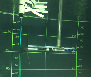
Figure 6. Picture of the turbine being tested in the flume with simultaneous flow measurements using the LDA system. The flag on the LDA mast is designed to break the structure of the vortex downstream of the mast and, therefore, to minimise vortex-induced vibration of the LDA probe.
3.1. Turbine specifications
The turbine used in the experiments was developed by IFREMER, with a strong focus on load and torque measurements. The blades are made of moulded carbon-fibre re-enforced plastic and are based on a NACA 63-418 profile. The turbine model is fitted with multiple force sensors (Gaurier, Germain & Facq Reference Gaurier, Germain and Facq2017). The root of each blade is instrumented with a load transducer measuring forces in the flapwise and lead-lag directions and bending moments along three orthogonal directions. Thrust and torque experienced by the rotor as a whole are also measured separately by a torque and thrust transducer. The load sensors were specially developed by the French company Sixaxes in collaboration with IFREMER. The load instrumentation described above is located, in terms of load path, upstream of the shaft seal so that the measurements are not affected by the friction associated with the seal. The transducers are therefore made waterproof as they have to be in contact with water. The turbine model generator is simulated by a permanent-magnet brushed motor fitted with a 1 : 26-ratio gearbox, both supplied by the company Maxon. The motor is controlled in speed to ensure near constant rotor speed. The closed-loop speed control relies on an encoder mounted at the back of the motor. Forty-eight shielded cables coming from the rotating turbine transducers are routed through a 52-channel slipring (as shown in figure 6), enabling the measurement signals to be transmitted to the stationary part of the turbine. These low-voltage signals are amplified by an electronic signal processing unit that is located outside of the turbine and of the water at the side of the flume.
The turbine performance and hydrodynamic characteristics, such as the power coefficient curve and the lift curve coefficients, are also presented in figure 7. The symbols in the power coefficient curve plot represent time-averaged measurements taken during the course of the present experiments, whereas the continuous dashed line provides a more complete picture of the turbine performance that was obtained during previous measurements reported in figure 4 of Gaurier et al. (Reference Gaurier, Germain and Facq2017). The two measurements are shown to be in excellent agreement. Moreover, in an attempt to estimate the hydrodynamic characteristics of the individual blade elements (hydrofoils), three tip-speed-ratio scenarios are considered and their collective chord Reynolds number,  $Re_c=\varOmega r c / \nu$, was found to range from
  $5 \times 10^4$ to
  $2 \times 10^5$. Using the potential flow solver, XFoil (Drela Reference Drela1989), we are able to extract the lift coefficient as a function of the angle of attack,
  $\alpha$, for the upper and lower bounds of chord Reynolds number values as shown on the right-hand side of figure 7. The slope of the lift curve coefficient,
  $\mathrm {d}C_L/\mathrm {d}\alpha$, is shown to be close to the theoretical value of
  $2{\rm \pi}$ up until stall, after which the slope decreases to a value approximately equal to unity. More details on the turbine model can be found in Gaurier et al. (Reference Gaurier, Germain and Facq2017) and Gaurier, Germain & Pinon (Reference Gaurier, Germain and Pinon2018) as well as in the appendix of this article, where a complete table of the radial distribution of the blade's geometric characteristics is provided.

Figure 7. (a) Power coefficient curve as a function of the tip-speed ratio,  $\lambda$, symbols showing the ensemble-average coefficients obtained from these measurements, whereas the continuous dashed lines shows the rotor's power coefficient curve according to Gaurier et al. (Reference Gaurier, Carlier, Germain, Pinon and Rivoalen2020) and the Betz limit. (b) Lift coefficient as a function of the angle of attack (in rad) for the NACA 63418 hydrofoil. Hydrofoil data for the different
  $Re_c$ have been calculated using XFoil (Drela Reference Drela1989) while the theoretical estimates for
  $\mathrm {d}C_L/\mathrm {d}\alpha$ are shown for reference.
3.2. Synchronous laser Doppler anemometry–turbine measurements
3.2.1. Flow measurements
We measure flow velocity using a two-dimensional optical fibre laser Doppler anemometry (LDA) system that comprises a FiberFlow transmitter and manipulators produced by the company Dantec and of two Genesis MX SLM series lasers made by the company Coherent. One of the lasers is green, with a wavelength of 514 nm, and the other is blue, with a wavelength of 488 nm. Laser Doppler anemometry measurements were taken using a downward-looking probe mounted on a motorised gantry, which allows automated probe movements in the vertical and transverse directions. The distance between the end of the probe and the measurement point is 500 mm, which allows for flow measurements close to the turbine with minimum interference with the flow experienced by the rotor. The LDA probe was set up so that the two velocity components measured were streamwise and transverse. The LDA sampling frequency is not constant, as each measurement takes place when a seeding particle crosses the measurement volume in the direction of interest (streamwise and/or transverse). In order to carry out FFT frequency analysis of the LDA measurements, the signal is first resampled at a constant frequency corresponding to the average of the non-constant sampling frequency of the raw signal. This signal processing operation is done on a test-run-by-test-run basis. For the LDA measurements used in this study, the average LDA sampling frequency associated with each run ranges from 601 Hz to 1351 Hz in the streamwise direction and from 435 Hz to 846 Hz in the transverse direction. The higher sampling frequency in the streamwise direction can be explained by the fact that the flow is predominantly streamwise; therefore, more seeding particles cross the measurement volume in that direction than in the transverse direction. For a given flow direction, the large range in average sampling frequency between runs is a result of the fact that the tests were carried out over a period of two weeks and the seeding particle concentration evolved over that period (seeding particles were actually added at some point between tests to ensure that the sampling frequency would not drop too low).
3.2.2. Data acquisition
All signals from the turbine sensors were logged using a National Instruments PXI express 4339 analogue voltage card mounted into a PXI express 1078 chassis also manufactured by National Instruments. The measurements were logged at 256 Hz and no hardware filtering was applied. For each run, the start of the turbine sensors measurements was triggered by the start of the LDA measurements, thus ensuring a synchronised start between the flow and turbine measurements.
4. A parametric study of the semi-analytical model
In § 2 we presented the derivation of our semi-analytical model for the power fluctuations’ PSD based on a lift linearisation approach and the RSS technique. The final PSD function (2.27) depends on a number of parameters that will ultimately affect the solution. In fact, three parameters are believed to have a significant impact on the results. These are the magnitude of the rotor tip-speed ratio,  $\lambda =\varOmega D/(2 U_{1\infty })$, the upstream streamwise integral length scale normalised by the rotor diameter,
  $D$,
$D$,  $L_{1\infty }/D$, and the axial induction factor,
  $a$, which affects the solution through the turbulence translation function,
  $s(\tau )$. By varying one of these parameters individually while keeping the other two constant, we may infer their effect on the PSD functions. For simplicity in (2.29), we have assumed that
  $c(r) \sqrt {\lambda ^*(r)^2+1}$ is constant across the blade and equal to unity while the amplitude,
  $A=\frac {3}{2} \rho (1-a)^2 ({\mathrm {d} C_L}/{\mathrm {d}\alpha } )U_{1\infty }^2=\frac {3}{2}(1-a)^2$, after setting all parameters other than the axial induction factor equal to unity. This representation of the rotor is not a realistic one and we will show later that these parameters are inter-connected and can have a great impact on the shape and magnitude of the final PSD functions.
Starting with the rotational speed effect in figure 8(a), we have plotted  $S_P(\,f)$ scaled by
  $f^{5/3}$ for different tip-speed ratios ranging from
  $\lambda =2$ to 20, taking
  $L_{1\infty }=D$ and the axial induction factor
  $a$ set equal to zero so that
  $x(\tau )=-U_{1\infty } \tau$. The use of pre-multiplied spectra (i.e.
  $f^{5/3}S(\,f)$) in figure 8(a) is intended to highlight the regions where low-pass filtering between the velocity and power fluctuations takes place. In addition, we should note that while the assumption of a zeroth axial induction factor and the extension of the tip-speed ratio range to larger values (e.g.
  $\lambda =20$) allow us to test our model's asymptotic behaviour, such scenarios are of little practical use. Both wind and tidal-stream turbines are designed to operate within a certain range of small tip-speed ratios (e.g.
  $\lambda <10$) and the axial induction factor would also depend on both tip-speed ratio and the rotor aero/hydrodynamics. Nonetheless, in figure 8(a) we observe that the power spectra are strongly impacted by an increase in the tip-speed-ratio value. In particular, as we increase
  $\lambda$, the power spectral densities reach a slope,
  $f^{-3/2-5/3}$, over the inertial sub-range before transitioning to the high-frequency BPF regime. Here, the power spectra are plotted against the normalised frequency,
  $f/f_T$, where
  $f_T=\varOmega /2 {\rm \pi}$; thus, it is important to notice that the normalised transition frequency appears to be the same irrespective of the tip-speed-ratio value. In addition, all cases experience a region in which
  $f^{5/3}S_P(\,f)$ remains constant, implying that in the lower inertial range, the low-pass filtering effect does not occur for a sub-range of the inertial frequency range. This is an effect of only the relative magnitude of the upstream turbulence integral length scale,
  $L_{1\infty }$, and the rotor diameter,
  $D$, which we will examine next. The increasing tip-speed ratio does not appear to have an effect on determining the frequency where low-pass filtering starts. The shift of the curves to lower relative frequencies (
 $\,f/f_T$) in figure 8(a) is merely an effect of frequency normalisation. This is better highlighted in figure 8(b), where the power spectra
  $S_P(\,f)$ are plotted against
  $f\kern0.5pt D/U_{1\infty }$ and it can be clearly seen that the filtering effect starts at the same frequency irrespective of the
  $\lambda$ value, which is around
  $f \approx U_{1\infty }/D$. In the same figure, we observe that the amplitude of the high-frequency spectral peaks remain unchanged with increasing tip-speed ratios. Their amplitudes are estimated to be around
  $1\,\%$ of the respective low-frequency amplitude. Yet, the spectral energy associated with these modes can be as large as 20 % of the overall spectral energy thanks to their presence in the higher-frequency regime.

Figure 8. Effect of the rotor's tip-speed ratio,  $\lambda$, on the power spectra. (a) Plots of the power spectral densities scaled by
  $f^{-5/3}$ and plotted against the relative frequency,
  $f/f_T$. (b) Power spectral density functions,
  $S_P(\,f)$, are plotted against the relative frequency,
  $f\kern0.5pt D/U_{1\infty }$, which reveals the fact that the onset of low-pass filtering is independent of the tip-speed-ratio value. Plots are shown for
  $\lambda =2$, 4, 6, 8, 10, 12, 16 and 20.
Next, we look at the effect of the integral length scale by gradually increasing the ratio  $L_{1\infty }/D$ from 0.05 to 10 (figure 9). The effect of the integral length scale on the fluctuations was found to affect both the low- and high-frequency range (e.g. BPF peaks). In particular, the amplitude of the spectral peaks was found to be smaller with increasing
  $L_{1\infty }/D$. On the other hand, we observed an increase of the low-frequency spectral amplitude for
  $f<U_{1\infty }/D$, as we increase the value of
  $L_{1\infty }/D$. In addition, for a smaller
  $L_{1\infty }/D$ ratio, the low-frequency ‘plateau’ region extends to higher frequencies; therefore, the energy cascade of the power fluctuations becomes shorter. Conversely, as
  $L_{1\infty }/D$ increases, the energy cascade of power fluctuations extends beyond the filtering frequency,
  $f \approx U_{1\infty }/D$, and reveals a region where the power spectra fall of as
  $f^{-5/3}$. We should also mention here that by increasing the integral length scale, the fast Fourier transforms exhibit numerical instabilities over the higher frequencies; therefore, a finer resolution is required to properly resolve all modes.

Figure 9. Power spectra plotted for increasing values of the ratio between the upstream integral turbulence length scale,  $L_{1\infty }$, and the rotor diameter,
  $D$. Plots are shown for different values of
  $L_{1\infty }/D=0.05$, 0.1, 0.25, 0.5, 1, 2, 5 and 10, whereas the tip-speed ratio and axial induction factor remain constant and equal to
  $\lambda =6$ and
  $a=0$, respectively.
Lastly, the impact of the induction factor and, therefore, the role of the rotor's blockage and turbulence distortion is examined as well. For our parametric analysis, we have chosen  $L_{1\infty }=D$ and
  $\lambda =7$, which are representative values that will yield a converged solution in terms of the rotational or upstream turbulence effects. To this end, we vary the induction factor from
  $a=0$ to 0.4 and present results for both the cross-correlation and power spectral density functions in figure 10. For clarity, we plotted only the solutions for
  $a=0$ and
  $a=0.4$, which are indicated in figure 10 as ‘no-induction’ and ‘induction’, respectively. With the increase of the axial induction factor, the rotor cross-correlation function is moved upward, as a result of the velocity delay that shows the effect at the intermediate time scales,
  $|\tau |>0.1$. For
  $\tau =0$, the two normalised cross-correlation functions attain a value of unity while as
  $\tau \rightarrow \infty$ the two solutions collapse, as shown in the zoomed-in plot of figure 10(a). This implies that blockage does not affect the interaction of the large flow variations with the rotor. The impact of the axial induction factor on the cross-correlation function is also shown to affect the shape of the derived PSD function. Inherently, the collapse between the cross-correlation function for small and large values of
  $|\tau |$ would mean that the low- and high-frequency spectral amplitudes will not be affected significantly as confirmed by figure 10(b). Conversely, the intermediate-frequency range is shown to be impacted the most, with the PSD being pushed downward. Moreover, for an induction factor of
  $a=0.4$, we were able to recover the
  $f^{-2}$ slope at the same range from the previously found
  $f^{-3/2}$. Therefore, it can be argued that the final low-pass filtering effect and the respective
  $f^{-11/3}$ scaling law stems not only from the angular velocity of the rotor (rotational effects) but also from the flow deceleration induced by the rotor's blockage.

Figure 10. The cross-correlation function and respective power spectra with and without considering the effect of inflow distortion. Results are shown for  $\lambda ={7}$,
  $L_{1\infty }/D={1}$ and taking an induction factor,
  $a={0.4}$. The power spectra in the right-hand side plot are scaled by
  $f^{-5/3}$.
5. Comparison with experiments
5.1. Distortion of the approaching turbulence
We start the comparison between the model and the experimental results by comparing the inflow velocity field at different locations upstream of the rotor. Measurements of the inflow velocity have been collected along the rotor axis and at the locations  $x_1/D=(-4,-3,-2,-1,-0.5,-0.15)$ upstream of the rotor for all three tip-speed-ratio cases,
  $\lambda =2$, 4 and 7. By excluding the near-rotor measurements (i.e.
  $x_1/D=-0.5$ and
  $-0.15$) to avoid the rotor's time scale interference, we may compute the upstream integral turbulence time scale,
 \begin{equation} T_{1\infty} = \int _0^\infty \frac{ \overline{u_1^\prime(t)u_1^\prime(t+\tau)} }{\overline{{u_1^\prime}^2}} \,\mathrm{d} \tau. \end{equation}
To obtain a representative value for the integral time scale,  $T_{1\infty }$, we use an ensemble-averaged estimator of the mean autocorrelation function,
  $\overline {u_1^\prime (t)u_1^\prime (t+\tau )}$, and integrate in time until it crosses zero for the first time (
 $\tau \approx 2.93\ \textrm {s}$). This limit has been chosen in an arbitrary fashion and one could extend integration to higher values of
  $\tau$. However, we have found that integration of the ensemble-averaged autocorrelation function beyond our selected value yields very small differences for the magnitude of the integral time scale. The ensemble average of the autocorrelation function together with all other recorded cases as well as the ensemble-average function's ‘zero-crossing’ point are shown in figure 11. For the calculation of the integral length scale, we invoke the ‘frozen turbulence’ assumption,
  $L_{1\infty }=U_{1\infty } T_{1\infty }$, where
  $T_{1\infty }$ is an integral time scale extracted from the temporal autocorrelation function,
  $\overline {u_1^\prime (t)u_1^\prime (t+\tau )}$. According to the present calculations, the integral length scale is found to be equal to
  $L_{1\infty }=0.7D$.

Figure 11. Autocorrelation function of the streamwise velocity fluctuations upstream of the rotor. The black thick solid line represents an ensemble average of the autocorrelation functions from all upstream locations and tip-speed ratios, whereas the vertical dashed line is the upper limit,  $\tau \approx 2.93\ \textrm {s}$, up to which the ensemble-average autocorrelation function is integrated in order to compute the integral time scale,
  $T_{1\infty }$.
Next, in figure 12 we present the mean velocity and r.m.s. of the velocity fluctuations both from measured and model predictions as a function of the non-dimensionalised distance,  $x_1/D$. The three tip-speed-ratio cases are presented separately, as the rotational speed of the turbine affects the axial induction factor,
  $a$, through an increasing thrust force,
  $(\lambda ,a)=(2, 0.13)$,
  $(4, 0.3)$ and
  $(7, 0.41)$. Nonetheless, in all cases the same pattern is observed. The mean velocity (
 $U_{1}/U_{1\infty }$) remains unchanged up until
  $x_1/D=-1$, after which it starts reducing to almost half its value as it reaches the rotor plane. This is confirmed by the analytical solution of Conway (Reference Conway1995). It is noticeable that Conway's model underpredicts the velocity reduction for
  $\lambda =2$, especially for smaller values of
  $x_1/D$. A possible explanation for this phenomenon is that the geometry of the nose cone is not taken into account in the model. Indeed, for
  $x_1/D=-0.5$ and
  $-0.15$, the distance between the LDA measurement volume and the tip of the nose cone is only 270 mm and 16 mm, respectively. Such a close proximity of the nose cone (especially for
  $x_1/D=-0.15$) will lower the velocity measured by the LDA system. The discrepancy between the model and the experimental measurements for low values of
  $x_1/D$ is also larger for
  $\lambda = 2$. At a higher tip-speed ratio, the reduction in streamwise flow velocity close to the upstream of the rotor is dominated by the effect of the rotor, which is taken into account by the model. Whereas for
  $\lambda =2$, the flow deceleration is comparatively lower and the effect of the nose cone becomes significant. Nevertheless, Conway's model provides an accurate enough solution for the mean upstream rotor velocity for
  $\lambda =4$ and 7. Likewise, for the r.m.s. of the velocity fluctuations, a similar picture is drawn with the velocity fluctuations reducing significantly more as they near the rotor. To model this behaviour, we have considered two approaches. The first considers a quasi-steady approach for the r.m.s. of the velocity fluctuations,
  $\overline {{u_1^\prime }^2}/\overline {{u_{1\infty }^\prime }^2}=\gamma ^2(x_1)$, whereas the second approach (plotted as a dashed line in figure 12b) uses the methodology of Milne & Graham (Reference Milne and Graham2019). The two approaches follow the same trend, with the latter appearing to be different only in the vicinity of the rotor. This is due to the fact that both the vorticity distortion (amplification of the low-frequency turbulence spectral content) and blockage effects can be captured by this model. Nonetheless, the good agreement between the two approaches and the experimental data validates our hypothesis regarding the quasi-steady behaviour of the velocity fluctuations presented in § 2.1.

Figure 12. (a) Mean normalised velocity,  $U_1/U_{1\infty }$, upstream of the rotor and (b) mean square intensity ratio,
  $\overline {{u_1^\prime }^2}/\overline {{u_{1\infty }^\prime }^2}$. Both quantities are plotted against the normalised upstream distance,
  $x_1/D$, and shown for all three tip-speed ratios. Symbols are the measurements, solid lines are the quasi-steady predictions and dashed lines follow the work of Milne & Graham (Reference Milne and Graham2019).
Looking at the inflow velocity spectra of figure 13, three operational cases are again presented. For each case, the streamwise velocity spectra are plotted for different locations upstream together with the undistorted and distorted theoretical spectra computed using the von Kármán (VK) model spectrum of (2.10). The distorted spectrum is taken at the closer location to the rotor ( $x_1/D={-0.15}$) for which we have measurements. As expected, the undistorted von Kármán spectrum is found to provide an excellent fit to the experimental data using the measured integral length scale,
  $L_{1\infty }=0.7D$, for all velocity spectra at locations
  $x_1/D<-0.5$. Conversely, the distorted velocity spectra show that the approach is only valid at the low-frequency regime and for the
  $\lambda ={4}$ and 7 cases. This is because, in general, our quasi-steady model becomes incapable of capturing the velocity spectra for higher frequencies,
  $f>U_{1\infty }/L_{1\infty }$, whereas for
  $\lambda ={2}$ the inference of the noise cone appears to have the same effect we pointed out previously when we presented the mean velocity and r.m.s. of the velocity fluctuations comparisons with the respective measured data.

Figure 13. Spectra of streamwise turbulent velocity in the inflow region at various distances upstream the rotor plane,  $x_1/D=(-0.15,-0.5,-1,-2)$, at hub height. Results are shown for all three tip-speed ratios (
 $\lambda =2$, 4 and 7).
5.2. Power spectra
We present a comparison between our semi-analytical solution and the experimentally measured PSD functions. Additionally, we will present a comparison with the PSD model of Tobin et al. (Reference Tobin, Zhu and Chamorro2015). Tobin et al. (Reference Tobin, Zhu and Chamorro2015) proposed a first-order stochastic ODE, which they derived using basic energy balance arguments,
 \begin{equation} \frac{\mathrm{d} P}{\mathrm{d} t} + \frac{P}{t_I} = \frac{1}{2 t_I}\rho C_P A u^3(t) ,\end{equation}
where  $t_I=I \varOmega /(2 Q)$ is a constant rotor inertial time scale. By solving the ODE using the impulse response function, Tobin et al. (Reference Tobin, Zhu and Chamorro2015) showed that the transfer function between the velocity and power fluctuation spectra approaches the
  $f^{-2}$ behaviour over the inertial and high-frequency regimes. In addition, they proposed using a second-order Butterworth filter for the transfer function between the power and velocity spectra and combined it with the von Kármán model velocity spectrum to finally obtain a model for the rotor's power spectrum,
 \begin{equation} S_P(\,f)=\frac{[3/2 C_p \rho A U_{1\infty}^2]^2}{\sqrt{1+(2f t_I)^4}}\frac{4\overline{u^{\prime 2}_{1\infty}} L_{1\infty}/U_{1 \infty} }{[1+70.8(\,f\kern0.5pt L_{1\infty}/U_{1 \infty})^2]^{5/6}}. \end{equation}
The proposed model spectrum effectively captures the low-pass filtering behaviour over higher frequencies; however, it does not predict the spectral peaks around the blade-passing frequencies. At the end of this section, we will show that Tobin's model agrees well with our semi-analytical, however only for ideal conditions and in the low and inertial-range frequencies.
Looking at the measured velocity and power power spectral densities of figure 14, we observe that indeed the low-pass filtering behaviour between power and velocity fluctuations exists and that the effect is more pronounced for the high tip-speed-ratio cases ( $\lambda =4$ and 7). A clearer picture of the three power spectral densities can be obtained by collapsing all data together (by dividing with the turbine frequency,
  $f_T=\varOmega /(2 {\rm \pi})$), as shown in figure 15(a). The collapsed spectral functions (shown on the left-hand side of the figure) confirm the existence of the three distinct regions: a low-frequency regime (I) in which power fluctuations follow those of the velocity, an intermediate regime (II), often coinciding with part of the inertial sub-range, in which the power fluctuation scale as
  $f^{-11/3}$, and a high-frequency regime (III) containing the BPF and their harmonics,
  $3f_T$,
  $6f_T$,
  $9 f_T$ and so on. Such characterisation of the power spectra is consistent with previous observations in both small- and large-scale experiments (Chamorro et al. Reference Chamorro, Hill, Morton, Ellis, Arndt and Sotiropoulos2013, Reference Chamorro, Lee, Olsen, Milliren, Marr, Arndt and Sotiropoulos2015; Tobin et al. Reference Tobin, Zhu and Chamorro2015). The presence of the BPF around multiples of
  $3f_T$ is independent of the vertical shear profile, as was shown numerically by Churchfield et al. (Reference Churchfield, Lee, Michalakes and Moriarty2012), and stems from the fact that power fluctuations are the result of torque fluctuations over all three turbine blades. A potential shift of the peaks away from the
  $3f_T$ frequency multiples would mean that one of the blades exhibits a different aero/hydrodynamic behaviour either by design (e.g. variation of shape/mass between blades) or by control (e.g. individual blade pitch). We may also notice that a critical frequency exists that separates regimes (II) and (III). This critical frequency also concurs for all three cases and it can approximately be placed at
  $f_c=3f_T/2$. This observation agrees with Chamorro et al. (Reference Chamorro, Hill, Morton, Ellis, Arndt and Sotiropoulos2013), who reported a linear relationship between
  $f_c$ and
  $f_T$. A more instructive way to encapsulate the physical characteristics of the three regimes can be obtained by defining a transfer function,
  $T(\,f/f_T)$, between the power and velocity spectral density functions as in Chamorro et al. (Reference Chamorro, Lee, Olsen, Milliren, Marr, Arndt and Sotiropoulos2015),
 \begin{equation} \mathcal{T_P}(\,f/f_T) = \frac{S_P(\,f/f_T)}{S_u(\,f/f_T)}. \end{equation}
Figure 15(b) shows that the measured transfer function for  $\lambda =4$ and
  $7$ collapse together, thereby further emphasising the existence of the three regimes. However, for
  $\lambda =2$, the spectral density function deviates from the previously mentioned description. In the lower-frequency regime, a positive cascade of spectral energy exists as
  $\mathrm {d}\mathcal {T}/\mathrm {d}f>0$. This is believed to be a result of the vortex shedding from individual blade elements that undergo dynamic stall with substantial flow detachment. Dynamic stall tends to transfer low-frequency velocity fluctuations toward the higher-frequency power spectral regime through lift fluctuations and instabilities introduced by the trailing- and leading-edge vortex shedding.

Figure 14. Power spectral density functions for the power and upstream velocity fluctuations (at hub height).

Figure 15. (a) Power spectral functions of the turbine power fluctuations,  $S_P(\,f)$, plotted against the normalised frequency,
  $f/f_T$. (b) The transfer function,
  $\mathcal {T}_P(\,f/f_T)$, as a function of the normalised frequency,
  $f/f_T$. In both plots, the measured PSD are plotted together with the model predictions from Tobin et al. (Reference Tobin, Zhu and Chamorro2015) and the present work.
In the same figures, we also plot the power spectra and the respective transfer functions using the present semi-analytical model. For our model calculations, we used 20 blade elements following the blade radial characteristics of table 1, whereas we extract the induction factors from the experimental data based on the mean thrust force. Finally, by monitoring the local angle of attack, we assign a lift coefficient slope to the local blade elements that switches between  $\mathrm {d}C_L/\mathrm {d}\alpha =2{\rm \pi}$ for
  $\alpha <\alpha _{{stall}}$ and
  $\mathrm {d}C_L/\mathrm {d}\alpha =1$ for
  $\alpha \ge \alpha _{stall}$. From figure 15(a) we can also see that our semi-analytical solution reproduces the power spectral peaks associated with the spectral amplification around the BPF and its harmonics exhibited by the experimental measurements. This is particularly true when it comes to the frequencies of these peaks. However, we notice that the model tends to overpredict the amplitude of the peaks. This is an inherent limitation of our semi-analytical model. The proposed linear relationship between inflow velocity fluctuations and the rotor's torque (see (2.17)), as well as the application of quasi-steady theory to the inflow velocity distortion, results in the overprediction of the interactions between small-scale turbulence and the blade aero/hydrodynamics. To this end, our model prediction for the energy content within these peaks is found to be
  $10\,\%$ more than the respective value found using the experimental data. In addition, for the optimal tip-speed-ratio case (
 $\lambda ={4}$), our model predicts that approximately 21 % of the overall energy is contained within the BPF modes, whereas using the experimental data reveals a smaller energy content that is approximately 8 % of the total energy.
Table 1. Blade dimensions based on NACA 63-418 profile. Here  $r$ is the local radius,
  $R$ the overall blade radius (362 mm),
  $c$ the chord length and
  $t$ the thickness.

In figure 15 we also plot the power spectra and the respective transfer functions using the Butterworth filter proposed by Tobin et al. (Reference Tobin, Zhu and Chamorro2015). To make the power spectra predictions using Tobin's model, we extracted the experimental power coefficients,  $C_P$, for the different tip-speed ratios, as well as compute the ‘inertial’ time scale based on the experimentally obtained, time-averaged torque and rotor speed. The two model predictions (present and Tobin's) are shown to exhibit an overall good agreement. However, important differences exist with the most significant one being that Tobin's model ignores the spectral amplification around the BPF and its harmonics. Moreover, the dependence of Tobin's transfer function on the mean power coefficient,
  $C_P$, appears to underpredict the low-frequency amplitude of the transfer function for
  $\lambda =7$ while overpredicting the one for
  $\lambda =2$. By revisiting our analysis in § 2, we may argue that the mean power coefficient is not a good estimator of the power fluctuations, as it does not provide any information on the aero/hydrodynamics of the individual blade elements. Conversely, the lift curve slope,
  $\mathrm {d} C_L/ \mathrm {d} \alpha$, provides a better estimate for the amplitude of the spectra, as shown by the ability of the current model to better capture the low-frequency amplitude of the experimental power spectral densities for all three tip-speed ratios. Surprisingly, the two models agree well for
  $\lambda =4$, which corresponds to the optimal rotor case (e.g. axial induction factor
  $a \sim 1/3$). For Tobin's model, the amplitude of the transfer function at the lower-frequency regime can be obtained by taking the limit of
  $f \rightarrow 0$ to obtain
 \begin{equation} \mathcal{T}_{Tobin}(0)= (\tfrac{3}{2} \rho C_p A U_{1\infty}^2)^2. \end{equation}
On the other hand, to obtain the low-frequency magnitude from the present model, we will need to take the limit of  $\tau \rightarrow \infty$ for the cross-correlation function,
  $R_{11}(r_1,r_2,\tau )$, which allows us to drop the time integral (Fourier transform) of the autocorrelation function to obtain
 \begin{equation} \mathcal{T}_{present}(0)=\left(\frac{3}{2} \rho (1-a)^2 \frac{\mathrm{d} C_L}{\mathrm{d} \alpha} U_{1\infty}^2 \right)^2 \left[ \int _0^R c(r) \sqrt{\lambda^*(r)^2+1} \mathrm{d} r \right]^2. \end{equation}
Dividing the two, we obtain
 \begin{equation} \frac{\mathcal{T}_{present}(0)}{\mathcal{T}_{Tobin}(0)}=\left[\frac{\mathrm{d} C_L}{\mathrm{d} \alpha} \frac{(1-a)^2}{A C_P} \int _0^R c(r) \sqrt{\lambda^*(r)^2+1} \, \mathrm{d} r \right]^2. \end{equation}
Finally, considering a theoretical power coefficient,  $C_P=4 \eta a (1-a)^2$, where
  $\eta$ is an efficiency coefficient (ratio between the actual
  $C_P$ and the theoretical Betz formula),
  $a$ is the axial induction factor,
  $\mathrm {d} C_L/\mathrm {d} \alpha = 2 {\rm \pi}$, and considering the blade's optimal design equations from Burton et al. (Reference Burton, Sharpe, Jenkins and Bossanyi2001, Chapter 3, equation (3.67)), we may equate the integrand to a constant value,
 \begin{equation} c(r) \sqrt{\lambda^*(r)^2+1} = \frac{2 {\rm \pi}}{3} \frac{4 a R}{\lambda C_L}, \end{equation}
which leads to the final
 \begin{equation} \frac{\mathcal{T}_{present}(0)}{\mathcal{T}_{Tobin}(0)}= \left( \frac{\rm \pi}{3}\frac{4}{\eta \lambda C_L} \right)^2 \approx 1 \end{equation}
for the optimal case, where  $\lambda ={4}$,
  $\eta =0.64$ and
  $C_L=1.5$. A final point can also be made for Tobin's ‘inertial’ time scale,
  $t_I$, which is proportional to the rotor's structural moment of inertia,
  $I$. This time scale controls the width of the transfer function's low-frequency ‘plateau’ region and, therefore, the critical frequency after which low-pass filtering starts. The ‘inertial’ time scale is found to be different for each tip-speed ratio, as the ratio between the mean torque,
  $Q$, and the mean rotor speed,
  $\varOmega$, varies with
  $\lambda$. Again, for all three cases, our semi-analytical model and that of Tobin et al. (Reference Tobin, Zhu and Chamorro2015) agree well only for the optimal tip-speed ratio,
  $\lambda =4$. In the present semi-analytical model, this critical ‘transition’ frequency is found to be
  $f_{{low\text {-}pass}} \approx 0.25 U_{1\infty }/D$ for
  $\lambda =4$. On the other hand, in Tobin's model low-pass filtering is activated when
  $2f t_I=1$. By substituting
  $f_{{low\text {-}pass}}$ into Tobin's model, we find that
  $t_I=4 D/(2 U_{1\infty }) \approx 1.8$, which agrees with the value found for
  $\lambda =2$ and 4 but not
  $\lambda =7$, which was found to be
  $t_I=8.16\ \textrm {s}$. This is caused by the fact that the mean torque,
  $Q$, is reduced when the rotor operates beyond its optimal tip-speed ratio, whereas the rotor speed continues to increase. Lastly, we should emphasise that our experiments were conducted at constant values of angular speed,
  $\varOmega$; hence, the rotational kinetic energy was also constant, and, therefore, the rotational inertia of the structure was found to be irrelevant.
6. Concluding remarks
In this work we examined the interaction between onset turbulence and a horizontal-axis turbine's power fluctuations under different tip-speed-ratio scenarios. The problem was studied both experimentally and through a novel semi-analytical model. The focus was on the power spectral density function of the power fluctuations (power spectra), and, in particular, the rotor's so-called low-pass-filtering behaviour in the inertial sub-range as well as the phenomena that affect it. The analysis showed that the turbine's rotational speed (i.e. tip-speed ratio), blade aero/hydrodynamic characteristics and distortion of the approaching turbulence all contribute to the filtering mechanism. In particular, we show that only a combined effect of inflow distortion and turbine rotation results in the experimentally observed  ${-11/3}$ scaling over the inertial sub-range. In addition, a detailed comparison with the present experimental data shows that the proposed semi-analytical model can also go beyond the inertial sub-region and effectively capture the behaviour around the blade-passing frequency and its high-frequency aliasing modes. To this end, the model also provides a pathway to calculating high-frequency torque fluctuations that are associated with rotor fatigue.
A parametric study for the proposed semi-analytical model highlighted the importance of the tip-speed ratio, upstream turbulence integral length scale and onset turbulence distortion/deceleration in shaping the power spectra. The magnitude of the tip-speed ratio was found to affect the intermediate- and higher-frequency regime. An increasing tip-speed ratio results in low-pass filtering of the power spectra in the inertial sub-range while it also generates pronounced spectral peaks around the blade-passing frequencies  $(3f_T,6f_T,9f_T,\ldots )$. Inherently, these spectral peaks will occur at higher frequencies as the tip-speed ratio increases. Conversely, the incipience of the low-pass filtering was found to be independent of the tip-speed-ratio magnitude and instead depends on the rotor diameter,
  $D$, and the undistorted upstream velocity,
  $U_{1\infty }$. The magnitude of the integral turbulence length scale,
  $L_{1\infty }$, was found to play a key role in determining the shape and the spectral amplitude in the low-frequency regime. For instance, larger values of
  $L_{1\infty }$ will extend the power spectra to low frequencies and may reveal a region where the
  ${-5/3}$ power law prevails. Such a region cannot be seen when
  $L_{1\infty } \leq D$ as low-pass filtering is active everywhere in the inertial sub-range. Again, the onset of low-pass filtering remains independent of the magnitude of the integral streamwise turbulence length scale. The
  ${-11/3}$ scaling law observed in our experimental results as well as in previous studies (Chamorro et al. Reference Chamorro, Lee, Olsen, Milliren, Marr, Arndt and Sotiropoulos2015; Tobin et al. Reference Tobin, Zhu and Chamorro2015) over the ‘filtered’ region of the inertial sub-range was obtained only when flow distortion was taken into account in our calculations.
Previous studies undertaken on the same problem (Chamorro et al. Reference Chamorro, Lee, Olsen, Milliren, Marr, Arndt and Sotiropoulos2015; Tobin et al. Reference Tobin, Zhu and Chamorro2015) have characterised the high-frequency regime as comprising uncorrelated and low-energy content disturbances. Dismissing the existence of the spectral peaks around the BPF in the high-frequency regime may result in ignoring a large amount of spectral energy contained within these frequencies. According to our model predictions, the BPF energy content can be as large as  $21\,\%$ of the overall spectral energy, whereas our experimental data suggest a figure closer to
  $8\,\%$. This percentage difference between the model and the experimental data stems from discrepancies around the BPF peaks. Our model overpredicts these peaks, as it lacks the ability to capture the unsteady blade-hydrodynamic phenomena present in these higher frequencies. Nonetheless, a number of studies (Stevens & Meneveau Reference Stevens and Meneveau2014; Bossuyt et al. Reference Bossuyt, Howland, Meneveau and Meyers2016, Reference Bossuyt, Meneveau and Meyers2017; Liu et al. Reference Liu, Jin, Tobin and Chamorro2017) have also suggested that time or space averages of the power output over multiple turbines (turbine arrays) may smear out the BPF peaks in the array-aggregate power spectra and give way to spectral peaks around the advective frequency (AF),
  $f_a \sim U_{1\infty }/S_x$, where
  $S_x$ is the distance between rows of turbines. An interesting analogy for the formation of these two types of spectral peaks (BPF and AF) can be drawn here as they are both a result of the velocity sampling. In the former (BPF), the spectral peaks happen because the velocity is sampled rotationally and with a constant angular speed, whereas in the latter (advective frequency), the velocity sampling corresponds to the convective travel time between rows having a constant spacing,
  $S_x$. Likewise, the
  ${-11/3}$ scaling law present in the inertial frequency range of the array-aggregate power spectra measured by Liu et al. (Reference Liu, Jin, Tobin and Chamorro2017) may also be partially attributed to the velocity sampling between rows of turbines. More importantly, the presence of the
  $f^{-2}$ scaling in the transfer function between the power and velocity spectra, which is prevalent across the low and inertial frequency regimes in the data reported by Liu et al. (Reference Liu, Jin, Tobin and Chamorro2017), can also be ascribed to the relatively small length scale to diameter ratio,
  $L_{1\infty }/D$, which was used in their experiments and allows the low-pass filtering effect to dominate. This is analogous to our model's spectral behaviour for a single turbine power output, and indicates the important role of the velocity sampling scale (e.g. frequency, length etc.) and its relative magnitude to the turbulence length scale, in shaping the spectra of a single turbine or multiple turbines’ array-aggregate power output.
Finally, this study seeks to provide a benchmark for comparison between high-fidelity computational fluid dynamics models with the ability of blade phase-resolving simulations, e.g. actuator line models (Churchfield et al. Reference Churchfield, Lee, Michalakes and Moriarty2012; Deskos, Laizet & Palacios Reference Deskos, Laizet and Palacios2020), and the presented solution for both wind and tidal energy applications. This will be complementary to many existing validation tests already undertaken by model developers that involve wake and performance statistics. Future studies will focus on time-series predictions of the power fluctuations by utilising the derived PSD functions.
Acknowledgements
The research leading to these results has received funding from the European Union Horizon 2020 Framework Program (H2020) under grant agreement no 731084. G.D. and M.G. would also like to acknowledge funding from EPSRC (grant number EP/R007470/1). G.D. was also supported by the U.S. Department of Energy (DOE) during the completion of this work. This work was authored in part by the National Renewable Energy Laboratory, operated by Alliance for Sustainable Energy, LLC, for the U.S. Department of Energy (DOE) under contract number DE-AC36-08GO28308. Funding provided by the U.S. Department of Energy Office of Energy Efficiency and Renewable Energy Wind Energy Technologies Office. The views expressed in the article do not necessarily represent the views of the DOE or the U.S. Government. The U.S. Government retains and the publisher, by accepting the article for publication, acknowledges that the U.S. Government retains a non-exclusive, paid-up, irrevocable, worldwide license to publish or reproduce the published form of this work, or allow others to do so, for U.S. Government purposes. Finally, several insightful comments and meaningful suggestions provided by the anonymous reviewers helped us improve the quality of the presentation and generalise the results of the present study.
Declaration of interests
The authors report no conflict of interest.
Appendix
The turbine used for these experiments is similar to that used in previous studies (Gaurier et al. Reference Gaurier, Germain and Pinon2018, Reference Gaurier, Germain and Facq2017). For completeness, we present in table 1 the chord and thickness sizes both in a dimensional and non-dimensional format, as well as the twist angle for each blade radius,  $r$.
$r$.


