1 Introduction
The flow over a rotating sphere in a quiescent fluid is present in many fields including meteorology and astrophysics, and a number of theoretical, experimental and numerical studies have been performed to investigate this flow. The slowly rotating case was initially analytically described in the limit of infinitely small Reynolds number
 $\mathit{Re}_{s}=\unicode[STIX]{x1D6FA}R^{2}/\unicode[STIX]{x1D708}$
by Stokes (Dennis, Singh & Ingham Reference Dennis, Singh and Ingham1980) where
$\mathit{Re}_{s}=\unicode[STIX]{x1D6FA}R^{2}/\unicode[STIX]{x1D708}$
by Stokes (Dennis, Singh & Ingham Reference Dennis, Singh and Ingham1980) where
 $\unicode[STIX]{x1D6FA}$
,
$\unicode[STIX]{x1D6FA}$
,
 $R$
and
$R$
and
 $\unicode[STIX]{x1D708}$
indicate the sphere angular velocity, the sphere radius and kinematic viscosity, respectively. Reynolds numbers of the order of
$\unicode[STIX]{x1D708}$
indicate the sphere angular velocity, the sphere radius and kinematic viscosity, respectively. Reynolds numbers of the order of
 $O(100)$
were studied analytically by Dennis et al. (Reference Dennis, Singh and Ingham1980) by means of a series expansion in terms of Gegenbauer functions. However, the determination of the coefficients of the series expansion becomes increasingly challenging as
$O(100)$
were studied analytically by Dennis et al. (Reference Dennis, Singh and Ingham1980) by means of a series expansion in terms of Gegenbauer functions. However, the determination of the coefficients of the series expansion becomes increasingly challenging as
 $\mathit{Re}_{s}$
is increased due to the growing importance of the nonlinear interactions between the terms of the series. Numerical solutions of the rotating-sphere problem became recently available (see for instance Calabretto et al.
Reference Calabretto, Levy, Denier and Mattner2015) but the simulation of the flow is increasingly challenging as the Reynolds number is increased, since a boundary layer is formed near the sphere surface. Instead of seeking a solution of the full Navier–Stokes equations, a feasible alternative is provided by boundary-layer theory, giving a leading description of what happens close to the surface where the angular momentum transfer takes place. The boundary-layer approximation of the rotating-sphere equations was initially proposed by Howarth (Reference Howarth1951), while a solution of them was proposed by Banks (Reference Banks1965) in terms of a series expansion of the distance from the pole. However, the series diverged close to the equator, so that a numerical solution of the equations was needed after a certain latitude (Garrett & Peake Reference Garrett and Peake2002). Furthermore, as the boundary-layer equations are parabolic, they will result in a non-zero azimuthal velocity at the equator, so that a collision between the two boundary layers coming from the poles must take place (Simpson & Stewartson Reference Simpson and Stewartson1982) with a new elliptic structure of the governing equations. Anyhow, the boundary-layer equations are expected to provide a good approximation of the flow near the sphere surface and away from the equator at high Reynolds numbers but the approximation will become increasingly inaccurate for small
$\mathit{Re}_{s}$
is increased due to the growing importance of the nonlinear interactions between the terms of the series. Numerical solutions of the rotating-sphere problem became recently available (see for instance Calabretto et al.
Reference Calabretto, Levy, Denier and Mattner2015) but the simulation of the flow is increasingly challenging as the Reynolds number is increased, since a boundary layer is formed near the sphere surface. Instead of seeking a solution of the full Navier–Stokes equations, a feasible alternative is provided by boundary-layer theory, giving a leading description of what happens close to the surface where the angular momentum transfer takes place. The boundary-layer approximation of the rotating-sphere equations was initially proposed by Howarth (Reference Howarth1951), while a solution of them was proposed by Banks (Reference Banks1965) in terms of a series expansion of the distance from the pole. However, the series diverged close to the equator, so that a numerical solution of the equations was needed after a certain latitude (Garrett & Peake Reference Garrett and Peake2002). Furthermore, as the boundary-layer equations are parabolic, they will result in a non-zero azimuthal velocity at the equator, so that a collision between the two boundary layers coming from the poles must take place (Simpson & Stewartson Reference Simpson and Stewartson1982) with a new elliptic structure of the governing equations. Anyhow, the boundary-layer equations are expected to provide a good approximation of the flow near the sphere surface and away from the equator at high Reynolds numbers but the approximation will become increasingly inaccurate for small
 $\mathit{Re}_{s}$
. To our knowledge, no attempt to develop a higher-order correction has been made so far.
$\mathit{Re}_{s}$
. To our knowledge, no attempt to develop a higher-order correction has been made so far.
The equatorial region deserves special attention. The experiments of Bowden & Lord (Reference Bowden and Lord1963), Hollerbach et al. (Reference Hollerbach, Wiener, Sullivan, Donnelly and Barenghi2002), Calabretto et al. (Reference Calabretto, Levy, Denier and Mattner2015) and the numerical simulations of Dennis et al. (Reference Dennis, Singh and Ingham1980) and Dennis & Duck (Reference Dennis and Duck1988) suggest a more complicate structure where the two boundary layers coming from the poles collide close to the equator, generating a boundary-layer eruption that subsequently becomes a radial jet (Squire Reference Squire, Görtler and Tollmien1955; Riley Reference Riley1962; Schwarz Reference Schwarz1963). Stewartson (Reference Stewartson and Görtler1958) proposed that the impinging region could be decomposed as an inviscid zone and as a very thin viscous region close to the equator plane and to the sphere surface, and described by planar Navier–Stokes equations. He did not however propose any solution for the inviscid region, despite the fact that it was described by a Poisson equation. Later, Smith & Duck (Reference Smith and Duck1977) proposed an asymptotic analysis suggesting a separation zone near the corner, but this separation region has not been observed in experiments and simulations, so that the characteristics of the impinging region remain unclear.
Clearly, the boundary-layer flows over rotating disks and spheres are closely related. Specifically, the rotating sphere is locally flat close to its poles and can be thought of as corresponding to small rotating disks in those regions. A natural question is then ‘how far does one have to move from a pole in order for the local sphere flow to cease sharing the stability properties of the disk?’. This question has received interest in the literature, most notably from Garrett who has shown that, like the rotating disk, the rotating sphere is locally both convectively and absolutely unstable at all latitudes for sufficiently large spin rates (Garrett & Peake Reference Garrett and Peake2002, Reference Garrett and Peake2004; Garrett Reference Garrett2010; Barrow & Garrett Reference Barrow and Garrett2013).
The focus of continued interest in the rotating disk has, in the last two decades, moved from the study of the spiral vortices in the transitional region (Gregory, Stuart & Walker Reference Gregory, Stuart and Walker1955; Hall Reference Hall1986; Malik Reference Malik1986), towards an attempt to explain the global behaviour of the system that results in the characteristically sharp onset of turbulence. It could be argued that this new focus began in the mid 1990s with the seminal hypothesis of Lingwood (Reference Lingwood1995) that local absolute instability plays a significant role in the promotion of a global response. Some years later, Davies & Carpenter (Reference Davies and Carpenter2003) showed by direct numerical simulations that, although the disk is indeed locally absolutely unstable, this does not lead to a linear global mode when the full non-parallel growth of the boundary layer is accounted for. That is, Lingwood’s initial hypothesis may have been unduly influenced by the use of the parallel-flow approximation in her linear analysis. At around the same time Pier (Reference Pier2003) demonstrated explicitly that a nonlinear approach is indeed required. However, he also went on to show that Lingwood’s local absolute instability fixes the onset of the nonlinear global mode which, in turn, has a secondary absolute instability that promotes the transition to turbulence. This result can be viewed as confirmation of Lingwood’s hypothesis but does also highlight that the rotating-disk flow is much more complicated than originally thought.
Refinements to the theoretical understanding of the precise transition mechanisms within the rotating-disk flow continue to develop with the community’s access to high-performance computing and some experimental evidence supporting the latest theoretical predictions do now exist (the interested reader is referred to the very latest developments due to Imayama, Alfredsson & Lingwood Reference Imayama, Alfredsson and Lingwood2012, Reference Imayama, Alfredsson and Lingwood2013, Reference Imayama, Alfredsson and Lingwood2014; Siddiqui et al. Reference Siddiqui, Mukund, Scott and Pier2013; Appelquist et al. Reference Appelquist, Schlatter, Alfredsson and Lingwood2015a ,Reference Appelquist, Schlatter, Alfredsson and Lingwood b ).
Motivated by the growing interest in the global mode over the rotating disk, Barrow, Garrett & Peake (Reference Barrow, Garrett and Peake2014) conducted a global stability analysis of the rotating-sphere boundary layer. Using the weakly non-parallel shear-flow formulation due to Monkewitz, Huerre & Chomaz (Reference Monkewitz, Huerre and Chomaz1993), they were able to infer the long-term global response from the strictly local absolute instability properties of the flow at each latitude. Their clear conclusion was that the sphere boundary-layer flow is in fact dictated by a linear global mode. Given the complicated nonlinear nature of the rotating-disk flow and the close relationship between the two geometries, this is a very surprising result.
In light of Davies & Carpenter’s conclusions, criticisms can be levelled against Barrow et al.’s approach to the global mode and Garrett’s earlier approaches to the convective instability: they rely on strictly local analyses which in turn rely on the parallel-flow approximation. This is the motivation for our present study where the parallel-flow approximation is now removed entirely from the analysis. While we present only the non-parallel convective analysis here, the opportunity is taken here to revisit the steady-flow solution over the rotating sphere. Unlike the disk, the spherical geometry is such that boundary layers originate separately in each hemisphere and travel symmetrically from each pole. The resulting collision at the equator leads to what is typically referred to as the boundary-layer eruption. All previous boundary-layer studies use the model due to Howarth (Reference Howarth1951) and Banks (Reference Banks1965) in which no account is made for this eruption (and also a number of additional viscous effects are neglected) in the steady flow, and here we present a more sophisticated model. For a detailed study of the equatorial jet resulting from the eruption, see Calabretto et al. (Reference Calabretto, Levy, Denier and Mattner2015).
The new steady-flow solution is presented in § 2 and the non-parallel formulation of the stability problem detailed in § 3. We consider the non-parallel corrections to the original convective analysis of Garrett & Peake (Reference Garrett and Peake2002) in § 4. Finally, a brief discussion of the local eigenmodes is given in § 5. Our conclusions are then drawn in § 6.
2 Basic flow analysis
Let us consider an isolated steadily rotating sphere in an otherwise quiescent medium. The problem is conveniently written in a fixed reference frame
 $(\unicode[STIX]{x1D703},\unicode[STIX]{x1D711},r)$
indicating the azimuthal, tangential and radial direction, respectively. The steady velocity field around the sphere is denoted by
$(\unicode[STIX]{x1D703},\unicode[STIX]{x1D711},r)$
indicating the azimuthal, tangential and radial direction, respectively. The steady velocity field around the sphere is denoted by
 $\boldsymbol{U}=(U,V,W)$
according to the adopted reference frame. Due to the axial symmetry of the flow, each velocity component is a function only of the radial and azimuthal position,
$\boldsymbol{U}=(U,V,W)$
according to the adopted reference frame. Due to the axial symmetry of the flow, each velocity component is a function only of the radial and azimuthal position,
 $r$
and
$r$
and
 $\unicode[STIX]{x1D703}$
, respectively. For the sake of notation, all the physical quantities will be denoted as functions of the azimuthal angle,
$\unicode[STIX]{x1D703}$
, respectively. For the sake of notation, all the physical quantities will be denoted as functions of the azimuthal angle,
 $\unicode[STIX]{x1D703}$
, and radial position,
$\unicode[STIX]{x1D703}$
, and radial position,
 $r$
, as first and second argument, respectively, and this order will be further maintained when scaled coordinates will be introduced. Here all the physical quantities are scaled by the density,
$r$
, as first and second argument, respectively, and this order will be further maintained when scaled coordinates will be introduced. Here all the physical quantities are scaled by the density,
 $\unicode[STIX]{x1D70C}$
, the angular velocity,
$\unicode[STIX]{x1D70C}$
, the angular velocity,
 $\unicode[STIX]{x1D6FA}$
, and the sphere radius,
$\unicode[STIX]{x1D6FA}$
, and the sphere radius,
 $R$
. The characteristic boundary-layer thickness (based on the kinematic viscosity,
$R$
. The characteristic boundary-layer thickness (based on the kinematic viscosity,
 $\unicode[STIX]{x1D708}$
),
$\unicode[STIX]{x1D708}$
),
 $\unicode[STIX]{x1D6FF}=(\unicode[STIX]{x1D708}/\unicode[STIX]{x1D6FA})^{1/2}\ll R$
, is also introduced for later use, together with the small perturbation parameter of the problem, namely
$\unicode[STIX]{x1D6FF}=(\unicode[STIX]{x1D708}/\unicode[STIX]{x1D6FA})^{1/2}\ll R$
, is also introduced for later use, together with the small perturbation parameter of the problem, namely
 $\unicode[STIX]{x1D716}=\unicode[STIX]{x1D6FF}/R$
. The mean-flow equations are
$\unicode[STIX]{x1D716}=\unicode[STIX]{x1D6FF}/R$
. The mean-flow equations are
 $$\begin{eqnarray}\frac{\unicode[STIX]{x2202}U}{\unicode[STIX]{x2202}\unicode[STIX]{x1D703}}+U\cot \unicode[STIX]{x1D703}+r\frac{\unicode[STIX]{x2202}W}{\unicode[STIX]{x2202}r}+2W=0,\end{eqnarray}$$
 $$\begin{eqnarray}\displaystyle & & \displaystyle \frac{U}{r}\frac{\unicode[STIX]{x2202}\boldsymbol{U}}{\unicode[STIX]{x2202}\unicode[STIX]{x1D703}}+W\frac{\unicode[STIX]{x2202}\boldsymbol{U}}{\unicode[STIX]{x2202}r}+\frac{1}{r}\left(\begin{array}{@{}c@{}}UW-V^{2}\cot \unicode[STIX]{x1D703}\\ VW+UV\cot \unicode[STIX]{x1D703}\\ -U^{2}-V^{2}\end{array}\right)=-\left(\begin{array}{@{}c@{}}\displaystyle \frac{1}{r}\frac{\unicode[STIX]{x2202}P}{\unicode[STIX]{x2202}\unicode[STIX]{x1D703}}\\ 0\\ \displaystyle \frac{\unicode[STIX]{x2202}P}{\unicode[STIX]{x2202}r}\end{array}\right)\nonumber\\ \displaystyle & & \displaystyle \quad +\,\frac{1}{r^{2}\,\mathit{Re}_{s}}\left[\frac{\unicode[STIX]{x2202}^{2}\boldsymbol{U}}{\unicode[STIX]{x2202}\unicode[STIX]{x1D703}^{2}}+\cot \unicode[STIX]{x1D703}\frac{\unicode[STIX]{x2202}\boldsymbol{U}}{\unicode[STIX]{x2202}\unicode[STIX]{x1D703}}+r^{2}\frac{\unicode[STIX]{x2202}^{2}\boldsymbol{U}}{\unicode[STIX]{x2202}r^{2}}+2r\frac{\unicode[STIX]{x2202}\boldsymbol{U}}{\unicode[STIX]{x2202}r}+\left(\begin{array}{@{}c@{}}\displaystyle 2\frac{\unicode[STIX]{x2202}W}{\unicode[STIX]{x2202}\unicode[STIX]{x1D703}}-U/\sin ^{2}\unicode[STIX]{x1D703}\\ -V/\sin ^{2}\unicode[STIX]{x1D703}\\ \displaystyle -2(W+U\cot \unicode[STIX]{x1D703})-2\frac{\unicode[STIX]{x2202}U}{\unicode[STIX]{x2202}\unicode[STIX]{x1D703}}\end{array}\right)\right]\!,\nonumber\\ \displaystyle & & \displaystyle\end{eqnarray}$$
where
 $\mathit{Re}_{s}=\unicode[STIX]{x1D6FA}R^{2}/\unicode[STIX]{x1D708}=(R/\unicode[STIX]{x1D6FF})^{2}=\unicode[STIX]{x1D716}^{-2}$
is the Reynolds number based on the sphere radius.
$\mathit{Re}_{s}=\unicode[STIX]{x1D6FA}R^{2}/\unicode[STIX]{x1D708}=(R/\unicode[STIX]{x1D6FF})^{2}=\unicode[STIX]{x1D716}^{-2}$
is the Reynolds number based on the sphere radius.

Figure 1. Schematic representation of the various regions subdividing the flow around the rotating sphere.
The base flow used for the stability calculations can be found from the solution of (2.1)–(2.2) but the simulations are expected to become increasingly more demanding as
 $\mathit{Re}_{s}$
increases, without gaining significant insight into the scaling properties of the flow. Therefore, a boundary-layer analysis is proposed here, where the flow is subdivided as schematically illustrated in figure 1 to make analytical progress. Historically, the analysis is usually started from the boundary layer along the sphere surface (Howarth Reference Howarth1951; Banks Reference Banks1965). By introducing the scaled coordinate
$\mathit{Re}_{s}$
increases, without gaining significant insight into the scaling properties of the flow. Therefore, a boundary-layer analysis is proposed here, where the flow is subdivided as schematically illustrated in figure 1 to make analytical progress. Historically, the analysis is usually started from the boundary layer along the sphere surface (Howarth Reference Howarth1951; Banks Reference Banks1965). By introducing the scaled coordinate
 $\unicode[STIX]{x1D702}=(r-1)/\unicode[STIX]{x1D716}$
and the inner asymptotic sequences
$\unicode[STIX]{x1D702}=(r-1)/\unicode[STIX]{x1D716}$
and the inner asymptotic sequences
 $$\begin{eqnarray}\displaystyle \left.\begin{array}{@{}c@{}}U=U_{0}+\unicode[STIX]{x1D716}U_{1}+O(\unicode[STIX]{x1D716}^{2}),\quad V=V_{0}+\unicode[STIX]{x1D716}V_{1}+O(\unicode[STIX]{x1D716}^{2}),\\ W=\unicode[STIX]{x1D716}W_{0}+\unicode[STIX]{x1D716}^{2}W_{1}+O(\unicode[STIX]{x1D716}^{3}),\quad P=\unicode[STIX]{x1D716}P_{0}+O(\unicode[STIX]{x1D716}^{2}),\end{array}\right\} & & \displaystyle\end{eqnarray}$$
it is possible to obtain the
 $O(1)$
problem
$O(1)$
problem
 $$\begin{eqnarray}\displaystyle & \displaystyle \frac{\unicode[STIX]{x2202}U_{0}}{\unicode[STIX]{x2202}\unicode[STIX]{x1D703}}+U_{0}\cot \unicode[STIX]{x1D703}+\frac{\unicode[STIX]{x2202}W_{0}}{\unicode[STIX]{x2202}\unicode[STIX]{x1D702}}=0, & \displaystyle\end{eqnarray}$$
 $$\begin{eqnarray}\displaystyle & \displaystyle U_{0}\frac{\unicode[STIX]{x2202}U_{0}}{\unicode[STIX]{x2202}\unicode[STIX]{x1D703}}+W_{0}\frac{\unicode[STIX]{x2202}U_{0}}{\unicode[STIX]{x2202}\unicode[STIX]{x1D702}}-V_{0}^{2}\cot \unicode[STIX]{x1D703}=\frac{\unicode[STIX]{x2202}^{2}U_{0}}{\unicode[STIX]{x2202}\unicode[STIX]{x1D702}^{2}}, & \displaystyle\end{eqnarray}$$
 $$\begin{eqnarray}\displaystyle & \displaystyle U_{0}\frac{\unicode[STIX]{x2202}V_{0}}{\unicode[STIX]{x2202}\unicode[STIX]{x1D703}}+W_{0}\frac{\unicode[STIX]{x2202}V_{0}}{\unicode[STIX]{x2202}\unicode[STIX]{x1D702}}+U_{0}V_{0}\cot \unicode[STIX]{x1D703}=\frac{\unicode[STIX]{x2202}^{2}V_{0}}{\unicode[STIX]{x2202}\unicode[STIX]{x1D702}^{2}}, & \displaystyle\end{eqnarray}$$
with
 $$\begin{eqnarray}P_{0}(\unicode[STIX]{x1D703},\unicode[STIX]{x1D702})=-\int _{\unicode[STIX]{x1D702}}^{\infty }(U_{0}^{2}+V_{0}^{2})\,\text{d}\unicode[STIX]{x1D701},\end{eqnarray}$$
and boundary conditions
 $$\begin{eqnarray}\displaystyle & U_{0}=V_{0}-\sin \unicode[STIX]{x1D703}=W_{0}=0\quad \text{for}~\unicode[STIX]{x1D702}=0, & \displaystyle\end{eqnarray}$$
 $$\begin{eqnarray}\displaystyle & \displaystyle U_{0}=V_{0}=\frac{\unicode[STIX]{x2202}W_{0}}{\unicode[STIX]{x2202}\unicode[STIX]{x1D702}}=0\quad \text{for}~\unicode[STIX]{x1D702}\rightarrow \infty . & \displaystyle\end{eqnarray}$$
The same set of equations and boundary conditions were proposed by Howarth (Reference Howarth1951) and solved by Banks (Reference Banks1965) with a series of powers of
 $\unicode[STIX]{x1D703}$
starting from the pole. The leading term of the series is the same as the von Kármán rotating-disk flow, underlining the similarity of the two flows near the pole. However, the series solution quickly diverges for large
$\unicode[STIX]{x1D703}$
starting from the pole. The leading term of the series is the same as the von Kármán rotating-disk flow, underlining the similarity of the two flows near the pole. However, the series solution quickly diverges for large
 $\unicode[STIX]{x1D703}$
and a numerical solution of the parabolic equations must instead be performed. The boundary conditions away from the wall assume that the flow outside the boundary-layer region is at rest with the exception of
$\unicode[STIX]{x1D703}$
and a numerical solution of the parabolic equations must instead be performed. The boundary conditions away from the wall assume that the flow outside the boundary-layer region is at rest with the exception of
 $W$
that has an outward velocity of order
$W$
that has an outward velocity of order
 $O(\unicode[STIX]{x1D716})$
that triggers the flow motion outside the boundary layer. Consequently, it is expected that the velocity outside the boundary layer is
$O(\unicode[STIX]{x1D716})$
that triggers the flow motion outside the boundary layer. Consequently, it is expected that the velocity outside the boundary layer is
 $O(\unicode[STIX]{x1D716})$
while the pressure field is
$O(\unicode[STIX]{x1D716})$
while the pressure field is
 $O(\unicode[STIX]{x1D716}^{2})$
.
$O(\unicode[STIX]{x1D716}^{2})$
.
The boundary-layer equations at order
 $O(\unicode[STIX]{x1D716})$
are
$O(\unicode[STIX]{x1D716})$
are
 $$\begin{eqnarray}\frac{\unicode[STIX]{x2202}U_{1}}{\unicode[STIX]{x2202}\unicode[STIX]{x1D703}}+U_{1}\cot \unicode[STIX]{x1D703}+\frac{\unicode[STIX]{x2202}W_{1}}{\unicode[STIX]{x2202}\unicode[STIX]{x1D702}}+2W_{0}+\unicode[STIX]{x1D702}\frac{\unicode[STIX]{x2202}W_{0}}{\unicode[STIX]{x2202}\unicode[STIX]{x1D702}}=0,\end{eqnarray}$$
 $$\begin{eqnarray}\displaystyle & & \displaystyle U_{0}\frac{\unicode[STIX]{x2202}U_{1}}{\unicode[STIX]{x2202}\unicode[STIX]{x1D703}}+U_{1}\frac{\unicode[STIX]{x2202}U_{0}}{\unicode[STIX]{x2202}\unicode[STIX]{x1D703}}+W_{0}\frac{\unicode[STIX]{x2202}U_{1}}{\unicode[STIX]{x2202}\unicode[STIX]{x1D702}}+W_{1}\frac{\unicode[STIX]{x2202}U_{0}}{\unicode[STIX]{x2202}\unicode[STIX]{x1D702}}+\unicode[STIX]{x1D702}W_{0}\frac{\unicode[STIX]{x2202}U_{0}}{\unicode[STIX]{x2202}\unicode[STIX]{x1D702}}+U_{0}W_{0}-2V_{0}V_{1}\cot \unicode[STIX]{x1D703}\nonumber\\ \displaystyle & & \displaystyle \quad =-\frac{\unicode[STIX]{x2202}P_{0}}{\unicode[STIX]{x2202}\unicode[STIX]{x1D703}}+\frac{\unicode[STIX]{x2202}^{2}U_{1}}{\unicode[STIX]{x2202}\unicode[STIX]{x1D702}^{2}}+\unicode[STIX]{x1D702}\frac{\unicode[STIX]{x2202}^{2}U_{0}}{\unicode[STIX]{x2202}\unicode[STIX]{x1D702}^{2}}+2\frac{\unicode[STIX]{x2202}U_{0}}{\unicode[STIX]{x2202}\unicode[STIX]{x1D702}},\end{eqnarray}$$
 $$\begin{eqnarray}\displaystyle & & \displaystyle U_{0}\frac{\unicode[STIX]{x2202}V_{1}}{\unicode[STIX]{x2202}\unicode[STIX]{x1D703}}+U_{1}\frac{\unicode[STIX]{x2202}V_{0}}{\unicode[STIX]{x2202}\unicode[STIX]{x1D703}}+W_{0}\frac{\unicode[STIX]{x2202}V_{1}}{\unicode[STIX]{x2202}\unicode[STIX]{x1D702}}+W_{1}\frac{\unicode[STIX]{x2202}V_{0}}{\unicode[STIX]{x2202}\unicode[STIX]{x1D702}}+\unicode[STIX]{x1D702}W_{0}\frac{\unicode[STIX]{x2202}V_{0}}{\unicode[STIX]{x2202}\unicode[STIX]{x1D702}}+V_{0}W_{0}+(U_{0}V_{1}+U_{1}V_{0})\cot \unicode[STIX]{x1D703}\nonumber\\ \displaystyle & & \displaystyle \quad =\frac{\unicode[STIX]{x2202}^{2}V_{1}}{\unicode[STIX]{x2202}\unicode[STIX]{x1D702}^{2}}+\unicode[STIX]{x1D702}\frac{\unicode[STIX]{x2202}^{2}V_{0}}{\unicode[STIX]{x2202}\unicode[STIX]{x1D702}^{2}}+2\frac{\unicode[STIX]{x2202}V_{0}}{\unicode[STIX]{x2202}\unicode[STIX]{x1D702}}.\end{eqnarray}$$
The above equations are linear in the perturbation terms and are driven by the boundary conditions and by some inhomogeneous terms coming from the
 $O(1)$
solution, including curvature effects. The associated boundary conditions are
$O(1)$
solution, including curvature effects. The associated boundary conditions are
 $U_{1}=V_{1}=W_{1}=0$
for
$U_{1}=V_{1}=W_{1}=0$
for
 $\unicode[STIX]{x1D702}=0$
, while for the outer edge the conditions depend on the outer flow and will be discussed later.
$\unicode[STIX]{x1D702}=0$
, while for the outer edge the conditions depend on the outer flow and will be discussed later.
Due to the parabolic nature of (2.4)–(2.6) and (2.10)–(2.12), the tangential velocity at the equator,
 $U_{0}(\unicode[STIX]{x03C0}/2,\unicode[STIX]{x1D702})$
, will not be zero, resulting in a viscous impinging wall jet with a lateral velocity
$U_{0}(\unicode[STIX]{x03C0}/2,\unicode[STIX]{x1D702})$
, will not be zero, resulting in a viscous impinging wall jet with a lateral velocity
 $V_{0}(\unicode[STIX]{x03C0}/2,\unicode[STIX]{x1D702})$
. Here, the azimuthal and radial changes happen with the same aspect ratio, suggesting an elliptic nature of the equations. Following Stewartson (Reference Stewartson and Görtler1958), it is possible to introduce now the scaled azimuthal position
$V_{0}(\unicode[STIX]{x03C0}/2,\unicode[STIX]{x1D702})$
. Here, the azimuthal and radial changes happen with the same aspect ratio, suggesting an elliptic nature of the equations. Following Stewartson (Reference Stewartson and Görtler1958), it is possible to introduce now the scaled azimuthal position
 $\unicode[STIX]{x1D6FD}=(\unicode[STIX]{x1D703}-\unicode[STIX]{x03C0}/2)/\unicode[STIX]{x1D716}$
, so that the following leading-order equations are determined for the impinging region
$\unicode[STIX]{x1D6FD}=(\unicode[STIX]{x1D703}-\unicode[STIX]{x03C0}/2)/\unicode[STIX]{x1D716}$
, so that the following leading-order equations are determined for the impinging region
 $$\begin{eqnarray}\displaystyle & \displaystyle \frac{\unicode[STIX]{x2202}U_{I}}{\unicode[STIX]{x2202}\unicode[STIX]{x1D6FD}}+\frac{\unicode[STIX]{x2202}W_{I}}{\unicode[STIX]{x2202}\unicode[STIX]{x1D702}}=0, & \displaystyle\end{eqnarray}$$
 $$\begin{eqnarray}\displaystyle & \displaystyle U_{I}\frac{\unicode[STIX]{x2202}U_{I}}{\unicode[STIX]{x2202}\unicode[STIX]{x1D6FD}}+W_{I}\frac{\unicode[STIX]{x2202}U_{I}}{\unicode[STIX]{x2202}\unicode[STIX]{x1D702}}=-\frac{\unicode[STIX]{x2202}P_{I}}{\unicode[STIX]{x2202}\unicode[STIX]{x1D6FD}}+\unicode[STIX]{x1D716}\left(\frac{\unicode[STIX]{x2202}^{2}U_{I}}{\unicode[STIX]{x2202}\unicode[STIX]{x1D6FD}^{2}}+\frac{\unicode[STIX]{x2202}^{2}U_{I}}{\unicode[STIX]{x2202}\unicode[STIX]{x1D702}^{2}}\right), & \displaystyle\end{eqnarray}$$
 $$\begin{eqnarray}\displaystyle & \displaystyle U_{I}\frac{\unicode[STIX]{x2202}V_{I}}{\unicode[STIX]{x2202}\unicode[STIX]{x1D6FD}}+W_{I}\frac{\unicode[STIX]{x2202}V_{I}}{\unicode[STIX]{x2202}\unicode[STIX]{x1D702}}=\unicode[STIX]{x1D716}\left(\frac{\unicode[STIX]{x2202}^{2}V_{I}}{\unicode[STIX]{x2202}\unicode[STIX]{x1D6FD}^{2}}+\frac{\unicode[STIX]{x2202}^{2}V_{I}}{\unicode[STIX]{x2202}\unicode[STIX]{x1D702}^{2}}\right), & \displaystyle\end{eqnarray}$$
 $$\begin{eqnarray}\displaystyle & \displaystyle U_{I}\frac{\unicode[STIX]{x2202}W_{I}}{\unicode[STIX]{x2202}\unicode[STIX]{x1D6FD}}+W_{I}\frac{\unicode[STIX]{x2202}W_{I}}{\unicode[STIX]{x2202}\unicode[STIX]{x1D702}}=-\frac{\unicode[STIX]{x2202}P_{I}}{\unicode[STIX]{x2202}\unicode[STIX]{x1D702}}+\unicode[STIX]{x1D716}\left(\frac{\unicode[STIX]{x2202}^{2}W_{I}}{\unicode[STIX]{x2202}\unicode[STIX]{x1D6FD}^{2}}+\frac{\unicode[STIX]{x2202}^{2}W_{I}}{\unicode[STIX]{x2202}\unicode[STIX]{x1D702}^{2}}\right), & \displaystyle\end{eqnarray}$$
where the subscript
 $I$
indicates velocity and pressure quantities in the impinging region (see figure 1). Differently from the boundary-layer region, all the velocity components are now
$I$
indicates velocity and pressure quantities in the impinging region (see figure 1). Differently from the boundary-layer region, all the velocity components are now
 $O(1)$
. Only the leading-order viscous terms are retained since they should generate new internal boundary layers along the surface of the sphere and along the equatorial plane of size
$O(1)$
. Only the leading-order viscous terms are retained since they should generate new internal boundary layers along the surface of the sphere and along the equatorial plane of size
 $O(\unicode[STIX]{x1D716}\sqrt{\unicode[STIX]{x1D716}})$
(Stewartson Reference Stewartson and Görtler1958). The associated boundary conditions are (at the leading order)
$O(\unicode[STIX]{x1D716}\sqrt{\unicode[STIX]{x1D716}})$
(Stewartson Reference Stewartson and Görtler1958). The associated boundary conditions are (at the leading order)
 $$\begin{eqnarray}\displaystyle & U_{I}=V_{I}-1=W_{I}=0\quad \text{for}~\unicode[STIX]{x1D702}=0, & \displaystyle\end{eqnarray}$$
 $$\begin{eqnarray}\displaystyle & \displaystyle U_{I}=\frac{\unicode[STIX]{x2202}V_{I}}{\unicode[STIX]{x2202}\unicode[STIX]{x1D6FD}}=\frac{\unicode[STIX]{x2202}W_{I}}{\unicode[STIX]{x2202}\unicode[STIX]{x1D6FD}}=0\quad \text{for}~\unicode[STIX]{x1D6FD}=0, & \displaystyle\end{eqnarray}$$
 $$\begin{eqnarray}\displaystyle & U_{I}-U_{0}(\unicode[STIX]{x03C0}/2,\unicode[STIX]{x1D702})=V_{I}-V_{0}(\unicode[STIX]{x03C0}/2,\unicode[STIX]{x1D702})=W_{I}=0\quad \text{for}~\unicode[STIX]{x1D6FD}\rightarrow -\infty . & \displaystyle\end{eqnarray}$$
In the region outside the boundary layers, an external inviscid flow is expected (Stewartson Reference Stewartson and Görtler1958; Smith & Duck Reference Smith and Duck1977) providing the upstream coupling needed for the elliptic region. By introducing a streamfunction
 $\unicode[STIX]{x1D6F9}_{I}$
, equations (2.13)–(2.16) reduce at the leading order to
$\unicode[STIX]{x1D6F9}_{I}$
, equations (2.13)–(2.16) reduce at the leading order to
 $$\begin{eqnarray}\frac{\unicode[STIX]{x2202}^{2}\unicode[STIX]{x1D6F9}_{I}}{\unicode[STIX]{x2202}\unicode[STIX]{x1D6FD}^{2}}+\frac{\unicode[STIX]{x2202}^{2}\unicode[STIX]{x1D6F9}_{I}}{\unicode[STIX]{x2202}\unicode[STIX]{x1D702}^{2}}=-\unicode[STIX]{x1D714}_{I}(\unicode[STIX]{x1D6F9}_{I}),\end{eqnarray}$$
with
 $$\begin{eqnarray}U_{I}=\frac{\unicode[STIX]{x2202}\unicode[STIX]{x1D6F9}_{I}}{\unicode[STIX]{x2202}\unicode[STIX]{x1D702}},\quad V_{I}=V_{I}(\unicode[STIX]{x1D6F9}_{I}),\quad W_{I}=-\frac{\unicode[STIX]{x2202}\unicode[STIX]{x1D6F9}_{I}}{\unicode[STIX]{x2202}\unicode[STIX]{x1D6FD}},\end{eqnarray}$$
where the vorticity
 $\unicode[STIX]{x1D714}_{I}$
and
$\unicode[STIX]{x1D714}_{I}$
and
 $V_{I}$
are constants along the streamlines. The boundary conditions of
$V_{I}$
are constants along the streamlines. The boundary conditions of
 $U_{I}=0$
along the sphere surface and
$U_{I}=0$
along the sphere surface and
 $\unicode[STIX]{x2202}V_{I}/\unicode[STIX]{x2202}\unicode[STIX]{x1D6FD}=\unicode[STIX]{x2202}W_{I}/\unicode[STIX]{x2202}\unicode[STIX]{x1D6FD}=\unicode[STIX]{x1D714}_{I}=0$
in the equatorial plane cannot be fulfilled by (2.20) and should be satisfied through the presence of local boundary layers. The solution of (2.20) has been discussed in the literature (Rubel Reference Rubel1983; Phares, Smedley & Flagan Reference Phares, Smedley and Flagan2000), but here it is further complicated by the presence of a recirculation region where the value of the vorticity is unknown, so that (2.20) cannot be solved directly and we need to solve (2.13)–(2.16) instead. Nevertheless the solution as
$\unicode[STIX]{x2202}V_{I}/\unicode[STIX]{x2202}\unicode[STIX]{x1D6FD}=\unicode[STIX]{x2202}W_{I}/\unicode[STIX]{x2202}\unicode[STIX]{x1D6FD}=\unicode[STIX]{x1D714}_{I}=0$
in the equatorial plane cannot be fulfilled by (2.20) and should be satisfied through the presence of local boundary layers. The solution of (2.20) has been discussed in the literature (Rubel Reference Rubel1983; Phares, Smedley & Flagan Reference Phares, Smedley and Flagan2000), but here it is further complicated by the presence of a recirculation region where the value of the vorticity is unknown, so that (2.20) cannot be solved directly and we need to solve (2.13)–(2.16) instead. Nevertheless the solution as
 $\unicode[STIX]{x1D702}\rightarrow \infty$
must approach the inflow, so that the outflow asymptotes to
$\unicode[STIX]{x1D702}\rightarrow \infty$
must approach the inflow, so that the outflow asymptotes to
 $$\begin{eqnarray}U_{I}=0,\quad V_{I}(\unicode[STIX]{x1D6FD})=V_{0}(\unicode[STIX]{x03C0}/2,-\unicode[STIX]{x1D6FD}),\quad W_{I}(\unicode[STIX]{x1D6FD})=U_{0}(\unicode[STIX]{x03C0}/2,-\unicode[STIX]{x1D6FD}).\end{eqnarray}$$
The presence of a separation and reattachment of the boundary layer near the equator suggests a more complex structure for the impinging region than the one proposed by Stewartson (Reference Stewartson and Görtler1958). Several research works have been devoted to this region in the attempt to describe the steady flow (Stewartson Reference Stewartson and Görtler1958; Smith & Duck Reference Smith and Duck1977) as well as the transient regime (Banks & Zaturska Reference Banks and Zaturska1979; Simpson & Stewartson Reference Simpson and Stewartson1982; Van Dommelen Reference Van Dommelen1990): the latter studies showed evidences of a finite-time singularity in the boundary-layer equations, suggesting a structure that might escape the description achievable with simple boundary-layer theory and parabolic equations. Smith & Duck (Reference Smith and Duck1977) proposed that the influence of the separation point should be felt much deeper than
 $\unicode[STIX]{x1D716}$
, and they developed an analysis based upon a new scaling coordinate
$\unicode[STIX]{x1D716}$
, and they developed an analysis based upon a new scaling coordinate
 $\unicode[STIX]{x1D703}=\unicode[STIX]{x1D703}_{0}+\unicode[STIX]{x1D716}^{6/7}\unicode[STIX]{x1D6FD}^{\prime }$
, where
$\unicode[STIX]{x1D703}=\unicode[STIX]{x1D703}_{0}+\unicode[STIX]{x1D716}^{6/7}\unicode[STIX]{x1D6FD}^{\prime }$
, where
 $\unicode[STIX]{x1D703}_{0}$
indicates the azimuthal position of the separation point. Some details about the upstream effect of the impinging region are proposed in the paper appendix. The result of the analysis is a correction to be applied as the equator is approached of the form given by (A 2). Such an analysis is not repeated for the reattachment point in the equatorial plane, so that here it will be assumed that the profiles (2.22) will be recovered downstream of the reattachment point and as
$\unicode[STIX]{x1D703}_{0}$
indicates the azimuthal position of the separation point. Some details about the upstream effect of the impinging region are proposed in the paper appendix. The result of the analysis is a correction to be applied as the equator is approached of the form given by (A 2). Such an analysis is not repeated for the reattachment point in the equatorial plane, so that here it will be assumed that the profiles (2.22) will be recovered downstream of the reattachment point and as
 $\unicode[STIX]{x1D702}\rightarrow \infty$
, as suggested by Stewartson (Reference Stewartson and Görtler1958).
$\unicode[STIX]{x1D702}\rightarrow \infty$
, as suggested by Stewartson (Reference Stewartson and Görtler1958).
Along the equatorial plane, radial effects will become increasingly important and the impinging-flow equations should be replaced by local parabolic equations as
 $$\begin{eqnarray}\displaystyle & \displaystyle \frac{\unicode[STIX]{x2202}U_{J}}{\unicode[STIX]{x2202}\unicode[STIX]{x1D6FD}}+r\frac{\unicode[STIX]{x2202}W_{J}}{\unicode[STIX]{x2202}r}+2W_{J}=0, & \displaystyle\end{eqnarray}$$
 $$\begin{eqnarray}\displaystyle & \displaystyle \frac{\unicode[STIX]{x2202}P_{J}}{\unicode[STIX]{x2202}\unicode[STIX]{x1D6FD}}=0, & \displaystyle\end{eqnarray}$$
 $$\begin{eqnarray}\displaystyle & \displaystyle U_{J}\frac{\unicode[STIX]{x2202}V_{J}}{\unicode[STIX]{x2202}\unicode[STIX]{x1D6FD}}+rW_{J}\frac{\unicode[STIX]{x2202}V_{J}}{\unicode[STIX]{x2202}r}+V_{J}W_{J}=\frac{1}{r}\frac{\unicode[STIX]{x2202}^{2}V_{J}}{\unicode[STIX]{x2202}\unicode[STIX]{x1D6FD}^{2}}, & \displaystyle\end{eqnarray}$$
 $$\begin{eqnarray}\displaystyle & \displaystyle U_{J}\frac{\unicode[STIX]{x2202}W_{J}}{\unicode[STIX]{x2202}\unicode[STIX]{x1D6FD}}+rW_{J}\frac{\unicode[STIX]{x2202}W_{J}}{\unicode[STIX]{x2202}r}-V_{J}^{2}=-r\frac{\unicode[STIX]{x2202}P_{J}}{\unicode[STIX]{x2202}r}+\frac{1}{r}\frac{\unicode[STIX]{x2202}^{2}W_{J}}{\unicode[STIX]{x2202}\unicode[STIX]{x1D6FD}^{2}}, & \displaystyle\end{eqnarray}$$
where
 $U=\unicode[STIX]{x1D716}U_{J}$
and
$U=\unicode[STIX]{x1D716}U_{J}$
and
 $V_{J}$
,
$V_{J}$
,
 $W_{J}=O(1)$
. The boundary conditions for the equatorial region are
$W_{J}=O(1)$
. The boundary conditions for the equatorial region are
 $$\begin{eqnarray}\displaystyle & \displaystyle U_{J}=\frac{\unicode[STIX]{x2202}V_{J}}{\unicode[STIX]{x2202}\unicode[STIX]{x1D6FD}}=\frac{\unicode[STIX]{x2202}W_{J}}{\unicode[STIX]{x2202}\unicode[STIX]{x1D6FD}}=0\quad \text{for}~\unicode[STIX]{x1D6FD}=0, & \displaystyle\end{eqnarray}$$
 $$\begin{eqnarray}\displaystyle & \displaystyle \frac{\unicode[STIX]{x2202}U_{J}}{\unicode[STIX]{x2202}\unicode[STIX]{x1D6FD}}=V_{J}=W_{J}=0\quad \text{for}~\unicode[STIX]{x1D6FD}\rightarrow -\infty . & \displaystyle\end{eqnarray}$$
Since the external pressure is of order
 $O(\unicode[STIX]{x1D716}^{2})$
, the pressure gradient can be removed from the analysis. Stewartson (Reference Stewartson and Görtler1958) suggested that this region could be described as a radial jet (Squire Reference Squire, Görtler and Tollmien1955; Schwarz Reference Schwarz1963), but the initial developing region differs due to the transfer of momentum between the radial and tangential velocity. A self-similar solution is possible in the limit of
$O(\unicode[STIX]{x1D716}^{2})$
, the pressure gradient can be removed from the analysis. Stewartson (Reference Stewartson and Görtler1958) suggested that this region could be described as a radial jet (Squire Reference Squire, Görtler and Tollmien1955; Schwarz Reference Schwarz1963), but the initial developing region differs due to the transfer of momentum between the radial and tangential velocity. A self-similar solution is possible in the limit of
 $r\rightarrow \infty$
with the assumption that the tangential velocity vanishes faster than the radial one. The self-similar solution is given by
$r\rightarrow \infty$
with the assumption that the tangential velocity vanishes faster than the radial one. The self-similar solution is given by
 $$\begin{eqnarray}U_{J}=-\frac{\sqrt{2}}{\overline{\unicode[STIX]{x1D6FF}}r}\tanh \left(\frac{\unicode[STIX]{x1D709}}{\sqrt{2}}\right),\quad W_{J}=\frac{1}{\overline{\unicode[STIX]{x1D6FF}}^{2}r}\,\text{sech}^{2}\left(\frac{\unicode[STIX]{x1D709}}{\sqrt{2}}\right),\end{eqnarray}$$
with
 $\unicode[STIX]{x1D709}=\unicode[STIX]{x1D6FD}/\overline{\unicode[STIX]{x1D6FF}}$
(Riley Reference Riley1962; Calabretto et al.
Reference Calabretto, Levy, Denier and Mattner2015). It should be noted that the characteristic variable
$\unicode[STIX]{x1D709}=\unicode[STIX]{x1D6FD}/\overline{\unicode[STIX]{x1D6FF}}$
(Riley Reference Riley1962; Calabretto et al.
Reference Calabretto, Levy, Denier and Mattner2015). It should be noted that the characteristic variable
 $\unicode[STIX]{x1D709}$
is constant in the radial direction. (This is only apparently against the conjecture of Stewartson (Reference Stewartson and Görtler1958): this apparent inconsistency is due to the different reference frames used as the thickness of the jet is constant in the
$\unicode[STIX]{x1D709}$
is constant in the radial direction. (This is only apparently against the conjecture of Stewartson (Reference Stewartson and Görtler1958): this apparent inconsistency is due to the different reference frames used as the thickness of the jet is constant in the
 $\unicode[STIX]{x1D6FD}$
–
$\unicode[STIX]{x1D6FD}$
–
 $r$
plane (since
$r$
plane (since
 $\unicode[STIX]{x1D6FD}$
is an angle), so that the jet will linearly expand in thickness.) Differently from in the radial-jet case, the presence of the tangential velocity in the equations leads to a transfer of momentum between the
$\unicode[STIX]{x1D6FD}$
is an angle), so that the jet will linearly expand in thickness.) Differently from in the radial-jet case, the presence of the tangential velocity in the equations leads to a transfer of momentum between the
 $V$
and
$V$
and
 $W$
components, so that
$W$
components, so that
 $\overline{\unicode[STIX]{x1D6FF}}$
cannot be assessed from the initial available momentum integral but rather as a result of the numerical simulation of (2.23)–(2.26) leading to
$\overline{\unicode[STIX]{x1D6FF}}$
cannot be assessed from the initial available momentum integral but rather as a result of the numerical simulation of (2.23)–(2.26) leading to
 $\overline{\unicode[STIX]{x1D6FF}}=1.5372$
. In both the numerical and self-similar solutions, the tangential velocity
$\overline{\unicode[STIX]{x1D6FF}}=1.5372$
. In both the numerical and self-similar solutions, the tangential velocity
 $\unicode[STIX]{x1D716}U_{J}(\unicode[STIX]{x1D6FD}\rightarrow -\infty ,r)$
is
$\unicode[STIX]{x1D716}U_{J}(\unicode[STIX]{x1D6FD}\rightarrow -\infty ,r)$
is
 $O(\unicode[STIX]{x1D716})$
and must be balanced in the outer layer.
$O(\unicode[STIX]{x1D716})$
and must be balanced in the outer layer.
As evident from the previous analyses, the flow outside the sphere boundary layer is inviscid and driven by the wall-normal velocity,
 $\unicode[STIX]{x1D716}W_{0}(\unicode[STIX]{x1D703},\unicode[STIX]{x1D702}\rightarrow \infty )$
, and the radial velocity outside of the equatorial radial jet,
$\unicode[STIX]{x1D716}W_{0}(\unicode[STIX]{x1D703},\unicode[STIX]{x1D702}\rightarrow \infty )$
, and the radial velocity outside of the equatorial radial jet,
 $\unicode[STIX]{x1D716}U_{J}(\unicode[STIX]{x1D6FD}\rightarrow -\infty ,r)$
, and indeed the velocity field in the outer layer is of order
$\unicode[STIX]{x1D716}U_{J}(\unicode[STIX]{x1D6FD}\rightarrow -\infty ,r)$
, and indeed the velocity field in the outer layer is of order
 $O(\unicode[STIX]{x1D716})$
. These ejection velocities are normal to the surface and do not carry tangential momentum, so that
$O(\unicode[STIX]{x1D716})$
. These ejection velocities are normal to the surface and do not carry tangential momentum, so that
 $V=0$
in the outer flow. Furthermore, the vorticity outside the boundary layer and radial jet is zero, so that the outside region is irrotational. It is possible to introduce a Stokes streamfunction,
$V=0$
in the outer flow. Furthermore, the vorticity outside the boundary layer and radial jet is zero, so that the outside region is irrotational. It is possible to introduce a Stokes streamfunction,
 $\unicode[STIX]{x1D6F9}_{O}(\unicode[STIX]{x1D703},r)$
, so that the velocity components are described by
$\unicode[STIX]{x1D6F9}_{O}(\unicode[STIX]{x1D703},r)$
, so that the velocity components are described by
 $$\begin{eqnarray}U_{O}=-\frac{1}{r\sin \unicode[STIX]{x1D703}}\frac{\unicode[STIX]{x2202}\unicode[STIX]{x1D6F9}_{O}}{\unicode[STIX]{x2202}r},\quad W_{O}=\frac{1}{r^{2}\sin \unicode[STIX]{x1D703}}\frac{\unicode[STIX]{x2202}\unicode[STIX]{x1D6F9}_{O}}{\unicode[STIX]{x2202}\unicode[STIX]{x1D703}}.\end{eqnarray}$$
Since the flow is irrotational, the equation that describes the outer region is
 $$\begin{eqnarray}\frac{\unicode[STIX]{x2202}^{2}\unicode[STIX]{x1D6F9}_{O}}{\unicode[STIX]{x2202}r^{2}}+\frac{1}{r^{2}}\frac{\unicode[STIX]{x2202}^{2}\unicode[STIX]{x1D6F9}_{O}}{\unicode[STIX]{x2202}\unicode[STIX]{x1D703}^{2}}-\frac{\cot \unicode[STIX]{x1D703}}{r^{2}}\frac{\unicode[STIX]{x2202}\unicode[STIX]{x1D6F9}_{O}}{\unicode[STIX]{x2202}\unicode[STIX]{x1D703}}=0,\end{eqnarray}$$
subjected to the boundary conditions
 $$\begin{eqnarray}\displaystyle \left.\begin{array}{@{}c@{}}\displaystyle \unicode[STIX]{x1D6F9}_{O}(0,r)=0,\quad \unicode[STIX]{x1D6F9}_{O}(\unicode[STIX]{x1D703},1)=\int _{0}^{\unicode[STIX]{x1D703}}\sin \unicode[STIX]{x1D712}W_{B}(\unicode[STIX]{x1D712},\unicode[STIX]{x1D702}\rightarrow \infty )\,\text{d}\unicode[STIX]{x1D712},\\ \displaystyle \unicode[STIX]{x1D6F9}_{O}\left(\frac{\unicode[STIX]{x03C0}}{2},r\right)=\int _{0}^{\unicode[STIX]{x03C0}/2}\sin \unicode[STIX]{x1D712}W_{0}(\unicode[STIX]{x1D712},\unicode[STIX]{x1D702}\rightarrow \infty )\,\text{d}\unicode[STIX]{x1D712}-\int _{1}^{r}\unicode[STIX]{x1D712}U_{J}(\unicode[STIX]{x1D6FD}\rightarrow -\infty ,\unicode[STIX]{x1D712})\,\text{d}\unicode[STIX]{x1D712},\\ \displaystyle \frac{\unicode[STIX]{x2202}^{2}\unicode[STIX]{x1D6F9}_{O}}{\unicode[STIX]{x2202}r^{2}}=0\quad \text{as}~r\rightarrow \infty .\end{array}\right\} & & \displaystyle\end{eqnarray}$$
The solution of problem (2.31), together with the boundary conditions (2.32), provides the external flow field needed to create the higher-order correction for the sphere boundary layer and equatorial jet. In particular, for the former, the outer edge boundary conditions can be determined for the
 $O(\unicode[STIX]{x1D716})$
problem (2.10)–(2.12) as
$O(\unicode[STIX]{x1D716})$
problem (2.10)–(2.12) as
 $$\begin{eqnarray}U_{1}(\unicode[STIX]{x1D703},\unicode[STIX]{x1D702})-U_{O}(\unicode[STIX]{x1D703},0)=V_{1}=0\quad \text{for}~\unicode[STIX]{x1D702}\rightarrow \infty ,\end{eqnarray}$$
together with the continuity equation enforced to determine
 $\unicode[STIX]{x2202}W_{1}/\unicode[STIX]{x2202}\unicode[STIX]{x1D702}$
at the outer edge.
$\unicode[STIX]{x2202}W_{1}/\unicode[STIX]{x2202}\unicode[STIX]{x1D702}$
at the outer edge.
2.1 Numerical solution of the mean-flow equations
To obtain the mean flow at the leading order, the boundary-layer equations (2.4)–(2.6) had to be solved first. These will provide the boundary-layer flow near the sphere surface and away from the impinging region (namely within a region
 $0\leqslant \unicode[STIX]{x1D703}<\unicode[STIX]{x03C0}/2-O(\unicode[STIX]{x1D716})$
). Similarly to Garrett & Peake (Reference Garrett and Peake2002), the Banks (Reference Banks1965) solution (here extended to the fifteenth order) is used until
$0\leqslant \unicode[STIX]{x1D703}<\unicode[STIX]{x03C0}/2-O(\unicode[STIX]{x1D716})$
). Similarly to Garrett & Peake (Reference Garrett and Peake2002), the Banks (Reference Banks1965) solution (here extended to the fifteenth order) is used until
 $\unicode[STIX]{x1D703}\approx 6^{\circ }$
, beyond which a finite-difference solution of the boundary-layer equations is proposed. This is based on a Newton method combined with a space-marching technique, significantly decreasing the computational time. The convergence criterion for the Newton method, implemented here and in the radial-jet flow, was imposed such that the correction velocity should be less than
$\unicode[STIX]{x1D703}\approx 6^{\circ }$
, beyond which a finite-difference solution of the boundary-layer equations is proposed. This is based on a Newton method combined with a space-marching technique, significantly decreasing the computational time. The convergence criterion for the Newton method, implemented here and in the radial-jet flow, was imposed such that the correction velocity should be less than
 $10^{-5}$
of the equatorial tangential velocity to exit the iterative loop. A second-order central finite-difference scheme was used to discretise the derivatives in the wall-normal direction, while a second-order backward scheme was adopted for the
$10^{-5}$
of the equatorial tangential velocity to exit the iterative loop. A second-order central finite-difference scheme was used to discretise the derivatives in the wall-normal direction, while a second-order backward scheme was adopted for the
 $\unicode[STIX]{x1D703}$
derivatives. The domain was discretised into 300 grid points uniformly distributed in the wall-normal direction between the sphere surface and
$\unicode[STIX]{x1D703}$
derivatives. The domain was discretised into 300 grid points uniformly distributed in the wall-normal direction between the sphere surface and
 $\unicode[STIX]{x1D702}_{max}=30$
, and 1500 uniformly distributed points between the pole and the equator. Figure 2 shows some of the obtained velocity profiles along the sphere surface. The wall jet in the azimuthal velocity is slowly established and tends to decelerate and rise as the equator is approached. On the other hand, both the radial and tangential velocities show instead a monotonic trend.
$\unicode[STIX]{x1D702}_{max}=30$
, and 1500 uniformly distributed points between the pole and the equator. Figure 2 shows some of the obtained velocity profiles along the sphere surface. The wall jet in the azimuthal velocity is slowly established and tends to decelerate and rise as the equator is approached. On the other hand, both the radial and tangential velocities show instead a monotonic trend.

Figure 2. Sphere boundary-layer velocity profiles from the numerical solution of (2.4)–(2.6) for
 $\unicode[STIX]{x1D703}=0^{\circ }$
,
$\unicode[STIX]{x1D703}=0^{\circ }$
,
 $15^{\circ }$
,
$15^{\circ }$
,
 $30^{\circ }$
,
$30^{\circ }$
,
 $45^{\circ }$
,
$45^{\circ }$
,
 $60^{\circ }$
,
$60^{\circ }$
,
 $75^{\circ }$
,
$75^{\circ }$
,
 $80^{\circ }$
,
$80^{\circ }$
,
 $85^{\circ }$
,
$85^{\circ }$
,
 $90^{\circ }$
according to the arrows’ direction. The profiles at
$90^{\circ }$
according to the arrows’ direction. The profiles at
 $\unicode[STIX]{x1D703}=0^{\circ }$
and
$\unicode[STIX]{x1D703}=0^{\circ }$
and
 $\unicode[STIX]{x1D703}=90^{\circ }$
are marked by thick lines.
$\unicode[STIX]{x1D703}=90^{\circ }$
are marked by thick lines.
After the impinging region, the equatorial jet takes place. Here the parabolic equations are solved again with a space-marching method based on a Newton iterative approach: a first-order backward differentiation scheme is used in the radial direction, while a central second-order scheme is used in the azimuthal direction. The latter is discretised in 200 grid points uniformly spaced between 0 and
 $\unicode[STIX]{x1D6FD}_{max}=20$
, while the radial domain is discretised in 200 grid points logarithmically spaced between
$\unicode[STIX]{x1D6FD}_{max}=20$
, while the radial domain is discretised in 200 grid points logarithmically spaced between
 $r_{min}=1.001$
(where the inlet condition is imposed) and
$r_{min}=1.001$
(where the inlet condition is imposed) and
 $r_{max}=20$
. As proposed by Stewartson (Reference Stewartson and Görtler1958), the outlet of the impinging region has the same shape as the inlet, although the symmetry boundary condition is not fulfilled. A sudden transient is then expected to adjust for the boundary condition, but at
$r_{max}=20$
. As proposed by Stewartson (Reference Stewartson and Görtler1958), the outlet of the impinging region has the same shape as the inlet, although the symmetry boundary condition is not fulfilled. A sudden transient is then expected to adjust for the boundary condition, but at
 $r=1.1$
the transient is terminated and the jet decays as expected (see figure 3). The tangential velocity decays faster than the radial one, allowing for the self-similar solution (2.29).
$r=1.1$
the transient is terminated and the jet decays as expected (see figure 3). The tangential velocity decays faster than the radial one, allowing for the self-similar solution (2.29).


The outer region is solved with a point Gauss–Seidel method based on second-order central finite differences in both the radial and azimuthal directions discretised with 1000 and 500 grid points, respectively. The outermost boundary was set again to
 $r_{max}=20$
. Figure 4 shows the blowing velocities outside of the sphere boundary layer and of the equatorial jet. These drive the potential flow outside and generate the streamline pattern shown in figure 5.
$r_{max}=20$
. Figure 4 shows the blowing velocities outside of the sphere boundary layer and of the equatorial jet. These drive the potential flow outside and generate the streamline pattern shown in figure 5.

Figure 4. Outer region velocities above the sphere boundary layer (a) and above the equatorial plane (b). Solid lines indicate
 $U$
, while dashed lines indicate
$U$
, while dashed lines indicate
 $W$
.
$W$
.

Figure 5. Iso-contours of the outer streamfunction
 $\unicode[STIX]{x1D6F9}_{O}$
.
$\unicode[STIX]{x1D6F9}_{O}$
.
From the outer streamfunction, the first-order perturbation velocity for the outer part of the sphere boundary layer can be determined (here shown in figure 4
a). The latter provides the outer boundary condition for the first-order problem that can be solved with the same numerical techniques used in the
 $O(1)$
problem (with the addition of some inhomogeneous terms) providing the first-order correction to the Howarth (Reference Howarth1951) theory. Figure 6 shows a collection of profiles of the first-order problem at the same azimuthal positions (except
$O(1)$
problem (with the addition of some inhomogeneous terms) providing the first-order correction to the Howarth (Reference Howarth1951) theory. Figure 6 shows a collection of profiles of the first-order problem at the same azimuthal positions (except
 $90^{\circ }$
) used in figure 2. Qualitatively, the correction implies a speed-up of the radial jet and a decrease of the tangential velocity diffusion.
$90^{\circ }$
) used in figure 2. Qualitatively, the correction implies a speed-up of the radial jet and a decrease of the tangential velocity diffusion.

Figure 6. Boundary-layer velocity profiles from the numerical solution of (2.10)–(2.12) for
 $\unicode[STIX]{x1D703}=0^{\circ }$
,
$\unicode[STIX]{x1D703}=0^{\circ }$
,
 $15^{\circ }$
,
$15^{\circ }$
,
 $30^{\circ }$
,
$30^{\circ }$
,
 $45^{\circ }$
,
$45^{\circ }$
,
 $60^{\circ }$
,
$60^{\circ }$
,
 $75^{\circ }$
,
$75^{\circ }$
,
 $80^{\circ }$
,
$80^{\circ }$
,
 $85^{\circ }$
according to the arrows’ direction. The profiles at
$85^{\circ }$
according to the arrows’ direction. The profiles at
 $\unicode[STIX]{x1D703}=0^{\circ }$
and
$\unicode[STIX]{x1D703}=0^{\circ }$
and
 $\unicode[STIX]{x1D703}=85^{\circ }$
are marked by thick lines.
$\unicode[STIX]{x1D703}=85^{\circ }$
are marked by thick lines.
In order to validate the predictions of the sphere boundary-layer velocity profiles from the perturbation theory, a finite-difference solution of the full equations (2.1)–(2.2) was performed. The numerical code solved the transformed equations proposed by Dennis et al. (Reference Dennis, Singh and Ingham1980) with a point Gauss–Seidel technique and second-order central finite differences to discretise the spatial derivatives. The domain was discretised into 300 grid points in the azimuthal direction and 200 in the
 $r^{-1}$
space between the sphere surface and
$r^{-1}$
space between the sphere surface and
 $r_{max}=\infty$
. A comparison between the finite-difference solution and the boundary-layer solution (for both the
$r_{max}=\infty$
. A comparison between the finite-difference solution and the boundary-layer solution (for both the
 $O(1)$
and the corrected one) is reported for three Reynolds numbers in figures 7–9. The corrected profiles include both the
$O(1)$
and the corrected one) is reported for three Reynolds numbers in figures 7–9. The corrected profiles include both the
 $O(\unicode[STIX]{x1D716})$
correction due to the Reynolds number effects and the
$O(\unicode[STIX]{x1D716})$
correction due to the Reynolds number effects and the
 $O(\unicode[STIX]{x1D716}^{6/7})$
correction near the equator. As is visible from the figure, the corrections improve the agreement between the predicted boundary-layer velocity profiles and the simulation results, especially when the Reynolds number is low and when the azimuth approaches
$O(\unicode[STIX]{x1D716}^{6/7})$
correction near the equator. As is visible from the figure, the corrections improve the agreement between the predicted boundary-layer velocity profiles and the simulation results, especially when the Reynolds number is low and when the azimuth approaches
 $\unicode[STIX]{x1D703}=\unicode[STIX]{x03C0}/2$
. The corrections are not able to deal properly with the region near the equator and therefore fail there, limiting their use to a range
$\unicode[STIX]{x1D703}=\unicode[STIX]{x03C0}/2$
. The corrections are not able to deal properly with the region near the equator and therefore fail there, limiting their use to a range
 $0\leqslant \unicode[STIX]{x1D703}\leqslant \unicode[STIX]{x03C0}/2-O(\unicode[STIX]{x1D716})$
.
$0\leqslant \unicode[STIX]{x1D703}\leqslant \unicode[STIX]{x03C0}/2-O(\unicode[STIX]{x1D716})$
.

Figure 7. Comparison of the azimuthal (a), tangential (b) and radial (c) velocities near the sphere surface for
 $\unicode[STIX]{x1D703}=10^{\circ }$
,
$\unicode[STIX]{x1D703}=10^{\circ }$
,
 $30^{\circ }$
,
$30^{\circ }$
,
 $50^{\circ }$
,
$50^{\circ }$
,
 $70^{\circ }$
,
$70^{\circ }$
,
 $80^{\circ }$
and
$80^{\circ }$
and
 $\mathit{Re}_{s}=500$
. (○) Numerical solution of the full equations, (– – –) solution of the boundary-layer equations (2.4)–(2.6), (——) perturbed boundary-layer solution.
$\mathit{Re}_{s}=500$
. (○) Numerical solution of the full equations, (– – –) solution of the boundary-layer equations (2.4)–(2.6), (——) perturbed boundary-layer solution.

Figure 8. Comparison of the azimuthal (a), tangential (b) and radial (c) velocities near the sphere surface for
 $\unicode[STIX]{x1D703}=10^{\circ }$
,
$\unicode[STIX]{x1D703}=10^{\circ }$
,
 $30^{\circ }$
,
$30^{\circ }$
,
 $50^{\circ }$
,
$50^{\circ }$
,
 $70^{\circ }$
,
$70^{\circ }$
,
 $80^{\circ }$
and
$80^{\circ }$
and
 $\mathit{Re}_{s}=1000$
. See figure 7 for the list of the used symbols.
$\mathit{Re}_{s}=1000$
. See figure 7 for the list of the used symbols.

Figure 9. Comparison of the azimuthal (a), tangential (b) and radial (c) velocities near the sphere surface for
 $\unicode[STIX]{x1D703}=10^{\circ }$
,
$\unicode[STIX]{x1D703}=10^{\circ }$
,
 $30^{\circ }$
,
$30^{\circ }$
,
 $50^{\circ }$
,
$50^{\circ }$
,
 $70^{\circ }$
,
$70^{\circ }$
,
 $80^{\circ }$
and
$80^{\circ }$
and
 $\mathit{Re}_{s}=1500$
. See figure 7 for the list of the used symbols.
$\mathit{Re}_{s}=1500$
. See figure 7 for the list of the used symbols.
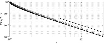
It is interesting to consider the evolution of the equatorial jet velocity field to assess whether the approximation regarding its inlet velocity distribution (given by (2.22)) affected its estimation. Figures 10 and 11 show the distribution of the radial and tangential velocity components along the equatorial plane. It is evident that a small disagreement is present near the sphere surface (mostly due to the absence of the boundary-layer analysis), but the same decay is quickly established and the jet solution represents indeed the outer limit when
 $\mathit{Re}_{s}\rightarrow \infty$
. Interestingly, the decay rate of the radial velocity goes as
$\mathit{Re}_{s}\rightarrow \infty$
. Interestingly, the decay rate of the radial velocity goes as
 $r^{-1}$
in agreement with the similarity solution (2.29), while the tangential velocity is faster and goes as
$r^{-1}$
in agreement with the similarity solution (2.29), while the tangential velocity is faster and goes as
 $r^{-2}$
following the similarity solution of Riley (Reference Riley1962).
$r^{-2}$
following the similarity solution of Riley (Reference Riley1962).


3 Formulation of the stability analysis
Let us consider now a small perturbation to the base state
 $(\boldsymbol{u},p)$
with
$(\boldsymbol{u},p)$
with
 $\boldsymbol{u}=(u,v,w)$
indicating the velocity perturbation and
$\boldsymbol{u}=(u,v,w)$
indicating the velocity perturbation and
 $p$
the pressure perturbation that can vary in time and space. By assuming the perturbation to be small, the continuity and linearised Navier–Stokes equations can be written. After subtracting the corresponding steady equations for the mean flow, it is possible to obtain the equations governing the perturbations
$p$
the pressure perturbation that can vary in time and space. By assuming the perturbation to be small, the continuity and linearised Navier–Stokes equations can be written. After subtracting the corresponding steady equations for the mean flow, it is possible to obtain the equations governing the perturbations
 $$\begin{eqnarray}\displaystyle & \displaystyle \frac{\unicode[STIX]{x2202}u}{\unicode[STIX]{x2202}\unicode[STIX]{x1D703}}+\cot \unicode[STIX]{x1D703}u+\frac{1}{\sin \unicode[STIX]{x1D703}}\frac{\unicode[STIX]{x2202}v}{\unicode[STIX]{x2202}\unicode[STIX]{x1D711}}+r\frac{\unicode[STIX]{x2202}w}{\unicode[STIX]{x2202}r}+2w=0, & \displaystyle\end{eqnarray}$$
 $$\begin{eqnarray}\displaystyle & \displaystyle \frac{\unicode[STIX]{x2202}\boldsymbol{u}}{\unicode[STIX]{x2202}t}+(\boldsymbol{U}\boldsymbol{\cdot }\unicode[STIX]{x1D735})\boldsymbol{u}+(\boldsymbol{u}\boldsymbol{\cdot }\unicode[STIX]{x1D735})\boldsymbol{U}=-\unicode[STIX]{x1D735}p+\frac{1}{\mathit{Re}_{s}}\unicode[STIX]{x1D6FB}^{2}\boldsymbol{u}, & \displaystyle\end{eqnarray}$$
where the various terms are given classically (Kundu, Cohen & Dowling Reference Kundu, Cohen and Dowling2016) by
 $$\begin{eqnarray}\displaystyle & \displaystyle (\boldsymbol{U}\boldsymbol{\cdot }\unicode[STIX]{x1D735})\boldsymbol{u}=\frac{U}{r}\frac{\unicode[STIX]{x2202}\boldsymbol{u}}{\unicode[STIX]{x2202}\unicode[STIX]{x1D703}}+\frac{V}{r\sin \unicode[STIX]{x1D703}}\frac{\unicode[STIX]{x2202}\boldsymbol{u}}{\unicode[STIX]{x2202}\unicode[STIX]{x1D711}}+W\frac{\unicode[STIX]{x2202}\boldsymbol{u}}{\unicode[STIX]{x2202}r}+\frac{1}{r}\left(\begin{array}{@{}c@{}}Uw-V\cot \unicode[STIX]{x1D703}v\\ Vw+V\cot \unicode[STIX]{x1D703}u\\ -Uu-Vv\end{array}\right), & \displaystyle\end{eqnarray}$$
 $$\begin{eqnarray}\displaystyle & \displaystyle (\boldsymbol{u}\boldsymbol{\cdot }\unicode[STIX]{x1D735})\boldsymbol{U}=\frac{u}{r}\frac{\unicode[STIX]{x2202}\boldsymbol{U}}{\unicode[STIX]{x2202}\unicode[STIX]{x1D703}}+w\frac{\unicode[STIX]{x2202}\boldsymbol{U}}{\unicode[STIX]{x2202}r}+\frac{1}{r}\left(\begin{array}{@{}c@{}}Wu-V\cot \unicode[STIX]{x1D703}v\\ Wv+U\cot \unicode[STIX]{x1D703}v\\ -Uu-Vv\end{array}\right), & \displaystyle\end{eqnarray}$$
 $$\begin{eqnarray}\displaystyle & \displaystyle \unicode[STIX]{x1D735}p=\left(\frac{1}{r}\frac{\unicode[STIX]{x2202}p}{\unicode[STIX]{x2202}\unicode[STIX]{x1D703}},\frac{1}{r\sin \unicode[STIX]{x1D703}}\frac{\unicode[STIX]{x2202}p}{\unicode[STIX]{x2202}\unicode[STIX]{x1D711}},\frac{\unicode[STIX]{x2202}p}{\unicode[STIX]{x2202}r}\right)^{\text{T}}, & \displaystyle\end{eqnarray}$$
 $$\begin{eqnarray}\displaystyle \unicode[STIX]{x1D6FB}^{2}\boldsymbol{u} & = & \displaystyle \frac{1}{r^{2}}\left\{\vphantom{\left({\displaystyle \frac{\unicode[STIX]{x2202}v}{\unicode[STIX]{x2202}\unicode[STIX]{x1D711}}}\right)^{\text{T}}}\frac{\unicode[STIX]{x2202}^{2}\boldsymbol{u}}{\unicode[STIX]{x2202}\unicode[STIX]{x1D703}^{2}}+\cot \unicode[STIX]{x1D703}\frac{\unicode[STIX]{x2202}\boldsymbol{u}}{\unicode[STIX]{x2202}\unicode[STIX]{x1D703}}+\frac{1}{\sin ^{2}\unicode[STIX]{x1D703}}\frac{\unicode[STIX]{x2202}^{2}\boldsymbol{u}}{\unicode[STIX]{x2202}\unicode[STIX]{x1D711}^{2}}+r^{2}\frac{\unicode[STIX]{x2202}^{2}\boldsymbol{u}}{\unicode[STIX]{x2202}r^{2}}+2r\frac{\unicode[STIX]{x2202}\boldsymbol{u}}{\unicode[STIX]{x2202}r}\right.\nonumber\\ \displaystyle & & \displaystyle +\left(-\frac{u}{\sin ^{2}\unicode[STIX]{x1D703}}+2\frac{\unicode[STIX]{x2202}w}{\unicode[STIX]{x2202}\unicode[STIX]{x1D703}}-\frac{2\cot \unicode[STIX]{x1D703}}{\sin \unicode[STIX]{x1D703}}\frac{\unicode[STIX]{x2202}v}{\unicode[STIX]{x2202}\unicode[STIX]{x1D711}},-\frac{v}{\sin ^{2}\unicode[STIX]{x1D703}}+\frac{2}{\sin \unicode[STIX]{x1D703}}\frac{\unicode[STIX]{x2202}w}{\unicode[STIX]{x2202}\unicode[STIX]{x1D711}}+\frac{2\cot \unicode[STIX]{x1D703}}{\sin \unicode[STIX]{x1D703}}\frac{\unicode[STIX]{x2202}u}{\unicode[STIX]{x2202}\unicode[STIX]{x1D711}},\right.\nonumber\\ \displaystyle & & \displaystyle \left.\!\!\left.-2(w+\cot \unicode[STIX]{x1D703}u)-2\frac{\unicode[STIX]{x2202}u}{\unicode[STIX]{x2202}\unicode[STIX]{x1D703}}-\frac{2}{\sin \unicode[STIX]{x1D703}}\frac{\unicode[STIX]{x2202}v}{\unicode[STIX]{x2202}\unicode[STIX]{x1D711}}\right)^{\!\text{T}}\right\}.\end{eqnarray}$$
As our primary interest lies in the near-wall region, the same stretched wall-normal coordinate,
 $\unicode[STIX]{x1D702}$
, is introduced as in § 2. Furthermore, as the radial velocity is
$\unicode[STIX]{x1D702}$
, is introduced as in § 2. Furthermore, as the radial velocity is
 $O(\unicode[STIX]{x1D716})$
compared to the azimuthal and tangential ones, the notation
$O(\unicode[STIX]{x1D716})$
compared to the azimuthal and tangential ones, the notation
 $W=\unicode[STIX]{x1D716}\overline{W}$
will be adopted for the mean wall-normal velocity, which results in a balanced continuity equation.
$W=\unicode[STIX]{x1D716}\overline{W}$
will be adopted for the mean wall-normal velocity, which results in a balanced continuity equation.
At this point, the modal assumption for the velocity and pressure perturbations is introduced in the form (Monkewitz et al. Reference Monkewitz, Huerre and Chomaz1993; Barrow et al. Reference Barrow, Garrett and Peake2014)
 $$\begin{eqnarray}\unicode[STIX]{x1D719}(\unicode[STIX]{x1D703},\unicode[STIX]{x1D711},\unicode[STIX]{x1D702},t)=\hat{\unicode[STIX]{x1D719}}(\unicode[STIX]{x1D703},\unicode[STIX]{x1D702})\exp \left\{\frac{\text{i}}{\unicode[STIX]{x1D716}}\left[n\unicode[STIX]{x1D711}-\unicode[STIX]{x1D714}t+\int _{\unicode[STIX]{x1D703}_{0}}^{\unicode[STIX]{x1D703}}\unicode[STIX]{x1D6FC}(\unicode[STIX]{x1D709})\,\text{d}\unicode[STIX]{x1D709}\right]\right\},\end{eqnarray}$$
where
 $n/\unicode[STIX]{x1D716}$
must be an integer number in order to ensure the periodicity in the tangential direction. It is illustrative to look at the continuity equation for the perturbation quantities
$n/\unicode[STIX]{x1D716}$
must be an integer number in order to ensure the periodicity in the tangential direction. It is illustrative to look at the continuity equation for the perturbation quantities
 $$\begin{eqnarray}\frac{1}{\unicode[STIX]{x1D716}}\left(\text{i}\unicode[STIX]{x1D6FC}\hat{u} +\frac{\text{i}n}{\sin \unicode[STIX]{x1D703}}\hat{v}+\frac{\unicode[STIX]{x2202}{\hat{w}}}{\unicode[STIX]{x2202}\unicode[STIX]{x1D702}}\right)+\frac{\unicode[STIX]{x2202}\hat{u} }{\unicode[STIX]{x2202}\unicode[STIX]{x1D703}}+\cot \unicode[STIX]{x1D703}\hat{u} +\unicode[STIX]{x1D702}\frac{\unicode[STIX]{x2202}{\hat{w}}}{\unicode[STIX]{x2202}\unicode[STIX]{x1D702}}+2{\hat{w}}=0.\end{eqnarray}$$
By assuming a perturbation expansion of the form
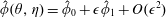 $\hat{\unicode[STIX]{x1D719}}(\unicode[STIX]{x1D703},\unicode[STIX]{x1D702})=\hat{\unicode[STIX]{x1D719}}_{0}+\unicode[STIX]{x1D716}\hat{\unicode[STIX]{x1D719}}_{1}+O(\unicode[STIX]{x1D716}^{2})$
, equation (3.8) leads to the problems at the orders
$\hat{\unicode[STIX]{x1D719}}(\unicode[STIX]{x1D703},\unicode[STIX]{x1D702})=\hat{\unicode[STIX]{x1D719}}_{0}+\unicode[STIX]{x1D716}\hat{\unicode[STIX]{x1D719}}_{1}+O(\unicode[STIX]{x1D716}^{2})$
, equation (3.8) leads to the problems at the orders
 $O(\unicode[STIX]{x1D716}^{-1})$
and
$O(\unicode[STIX]{x1D716}^{-1})$
and
 $O(1)$
 $$\begin{eqnarray}\displaystyle & \displaystyle \text{i}\unicode[STIX]{x1D6FC}\hat{u} _{0}+\text{i}\unicode[STIX]{x1D6FD}\hat{v}_{0}+\frac{\unicode[STIX]{x2202}{\hat{w}}_{0}}{\unicode[STIX]{x2202}\unicode[STIX]{x1D702}}=0\quad \text{with}~\unicode[STIX]{x1D6FD}=\frac{n}{\sin \unicode[STIX]{x1D703}}, & \displaystyle\end{eqnarray}$$
 $$\begin{eqnarray}\displaystyle & \displaystyle \text{i}\unicode[STIX]{x1D6FC}\hat{u} _{1}+\text{i}\unicode[STIX]{x1D6FD}\hat{v}_{1}+\frac{\unicode[STIX]{x2202}{\hat{w}}_{1}}{\unicode[STIX]{x2202}\unicode[STIX]{x1D702}}=-\left(\frac{\unicode[STIX]{x2202}\hat{u} _{0}}{\unicode[STIX]{x2202}\unicode[STIX]{x1D703}}+\cot \unicode[STIX]{x1D703}\hat{u} _{0}+\unicode[STIX]{x1D702}\frac{\unicode[STIX]{x2202}{\hat{w}}_{0}}{\unicode[STIX]{x2202}\unicode[STIX]{x1D702}}+2{\hat{w}}_{0}\right). & \displaystyle\end{eqnarray}$$
By introducing the state vector
 $\boldsymbol{q}=(\hat{u} ,\hat{v},{\hat{w}},\hat{p})^{\text{T}}$
, it is possible to write down the stability equations at the orders
$\boldsymbol{q}=(\hat{u} ,\hat{v},{\hat{w}},\hat{p})^{\text{T}}$
, it is possible to write down the stability equations at the orders
 $O(\unicode[STIX]{x1D716}^{-1})$
and
$O(\unicode[STIX]{x1D716}^{-1})$
and
 $O(1)$
as
$O(1)$
as
 $$\begin{eqnarray}\displaystyle & {\mathcal{L}}\boldsymbol{q}_{0}=\mathbf{0}, & \displaystyle\end{eqnarray}$$
 $$\begin{eqnarray}\displaystyle & {\mathcal{L}}\boldsymbol{q}_{1}=-{\mathcal{H}}\boldsymbol{q}_{0}, & \displaystyle\end{eqnarray}$$
where the operators
 ${\mathcal{L}}$
and
${\mathcal{L}}$
and
 ${\mathcal{H}}$
are given by
${\mathcal{H}}$
are given by
 $$\begin{eqnarray}{\mathcal{L}}=\left[-\text{i}\unicode[STIX]{x1D714}+\text{i}\unicode[STIX]{x1D6FC}U+\text{i}\unicode[STIX]{x1D6FD}V-\frac{1}{\unicode[STIX]{x1D716}\mathit{Re}_{s}}\left(\frac{\unicode[STIX]{x2202}^{2}}{\unicode[STIX]{x2202}\unicode[STIX]{x1D702}^{2}}-\unicode[STIX]{x1D6FC}^{2}-\unicode[STIX]{x1D6FD}^{2}\right)\right]\unicode[STIX]{x1D64C}+\left(\begin{array}{@{}cccc@{}}0 & 0 & {\displaystyle \frac{\unicode[STIX]{x2202}U}{\unicode[STIX]{x2202}\unicode[STIX]{x1D702}}} & \text{i}\unicode[STIX]{x1D6FC}\\ 0 & 0 & {\displaystyle \frac{\unicode[STIX]{x2202}V}{\unicode[STIX]{x2202}\unicode[STIX]{x1D702}}} & \text{i}\unicode[STIX]{x1D6FD}\\ 0 & 0 & 0 & {\displaystyle \frac{\unicode[STIX]{x2202}}{\unicode[STIX]{x2202}\unicode[STIX]{x1D702}}}\\ \text{i}\unicode[STIX]{x1D6FC} & \text{i}\unicode[STIX]{x1D6FD} & {\displaystyle \frac{\unicode[STIX]{x2202}}{\unicode[STIX]{x2202}\unicode[STIX]{x1D702}}} & 0\end{array}\right),\end{eqnarray}$$
 $$\begin{eqnarray}\displaystyle {\mathcal{H}} & = & \displaystyle \left[\text{i}\unicode[STIX]{x1D702}(-2\unicode[STIX]{x1D714}+\unicode[STIX]{x1D6FC}U+\unicode[STIX]{x1D6FD}V)+U\frac{\unicode[STIX]{x2202}}{\unicode[STIX]{x2202}\unicode[STIX]{x1D703}}+\overline{W}\frac{\unicode[STIX]{x2202}}{\unicode[STIX]{x2202}\unicode[STIX]{x1D702}}\right.\nonumber\\ \displaystyle & & \displaystyle -\left.\frac{1}{\unicode[STIX]{x1D716}\mathit{Re}_{s}}\left(2\text{i}\unicode[STIX]{x1D6FC}\frac{\unicode[STIX]{x2202}}{\unicode[STIX]{x2202}\unicode[STIX]{x1D703}}+\text{i}\frac{\unicode[STIX]{x2202}\unicode[STIX]{x1D6FC}}{\unicode[STIX]{x2202}\unicode[STIX]{x1D703}}+\text{i}\unicode[STIX]{x1D6FC}\cot \unicode[STIX]{x1D703}+2\unicode[STIX]{x1D702}\frac{\unicode[STIX]{x2202}^{2}}{\unicode[STIX]{x2202}\unicode[STIX]{x1D702}^{2}}+2\frac{\unicode[STIX]{x2202}}{\unicode[STIX]{x2202}\unicode[STIX]{x1D702}}\right)\right]\!\unicode[STIX]{x1D64C}\nonumber\\ \displaystyle & & \displaystyle +\left(\begin{array}{@{}cccc@{}}{\displaystyle \frac{\unicode[STIX]{x2202}U}{\unicode[STIX]{x2202}\unicode[STIX]{x1D703}}} & -2V\cot \unicode[STIX]{x1D703} & 2\unicode[STIX]{x1D702}{\displaystyle \frac{\unicode[STIX]{x2202}U}{\unicode[STIX]{x2202}\unicode[STIX]{x1D702}}}+U & \text{i}\unicode[STIX]{x1D702}\unicode[STIX]{x1D6FC}+{\displaystyle \frac{\unicode[STIX]{x2202}}{\unicode[STIX]{x2202}\unicode[STIX]{x1D703}}}\\ {\displaystyle \frac{\unicode[STIX]{x2202}V}{\unicode[STIX]{x2202}\unicode[STIX]{x1D703}}}+V\cot \unicode[STIX]{x1D703} & U\cot \unicode[STIX]{x1D703} & 2\unicode[STIX]{x1D702}{\displaystyle \frac{\unicode[STIX]{x2202}V}{\unicode[STIX]{x2202}\unicode[STIX]{x1D702}}}+V & \text{i}\unicode[STIX]{x1D702}\unicode[STIX]{x1D6FD}\\ -2U & -2V & {\displaystyle \frac{\unicode[STIX]{x2202}\overline{W}}{\unicode[STIX]{x2202}\unicode[STIX]{x1D702}}} & 2\unicode[STIX]{x1D702}{\displaystyle \frac{\unicode[STIX]{x2202}}{\unicode[STIX]{x2202}\unicode[STIX]{x1D702}}}\\ \cot \unicode[STIX]{x1D703}+{\displaystyle \frac{\unicode[STIX]{x2202}}{\unicode[STIX]{x2202}\unicode[STIX]{x1D703}}} & 0 & \unicode[STIX]{x1D702}{\displaystyle \frac{\unicode[STIX]{x2202}}{\unicode[STIX]{x2202}\unicode[STIX]{x1D702}}}+2 & 0\end{array}\right)\nonumber\\ \displaystyle & & \displaystyle -\,\frac{2\text{i}}{\unicode[STIX]{x1D716}\mathit{Re}_{s}}\left(\begin{array}{@{}cccc@{}}0 & -\unicode[STIX]{x1D6FD}\cot \unicode[STIX]{x1D703} & \unicode[STIX]{x1D6FC} & 0\\ \unicode[STIX]{x1D6FD}\cot \unicode[STIX]{x1D703} & 0 & \unicode[STIX]{x1D6FD} & 0\\ -\unicode[STIX]{x1D6FC} & -\unicode[STIX]{x1D6FD} & 0 & 0\\ 0 & 0 & 0 & 0\end{array}\right),\end{eqnarray}$$
and the matrix
 $\unicode[STIX]{x1D64C}$
defined as
$\unicode[STIX]{x1D64C}$
defined as
 $$\begin{eqnarray}\unicode[STIX]{x1D64C}=\left(\begin{array}{@{}cccc@{}}1 & 0 & 0 & 0\\ 0 & 1 & 0 & 0\\ 0 & 0 & 1 & 0\\ 0 & 0 & 0 & 0\end{array}\right).\end{eqnarray}$$
Since the differential operators in (3.11) do not depend on
 $\unicode[STIX]{x1D703}$
, the solution must be an eigenfunction of the form
$\unicode[STIX]{x1D703}$
, the solution must be an eigenfunction of the form
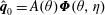 $\hat{\boldsymbol{q}}_{0}=A(\unicode[STIX]{x1D703})\unicode[STIX]{x1D731}(\unicode[STIX]{x1D703},\unicode[STIX]{x1D702})$
. The unknown function
$\hat{\boldsymbol{q}}_{0}=A(\unicode[STIX]{x1D703})\unicode[STIX]{x1D731}(\unicode[STIX]{x1D703},\unicode[STIX]{x1D702})$
. The unknown function
 $A(\unicode[STIX]{x1D703})$
can be found from the Fredholm alternative theorem applied to (3.12) leading to the condition
$A(\unicode[STIX]{x1D703})$
can be found from the Fredholm alternative theorem applied to (3.12) leading to the condition
 $$\begin{eqnarray}\int _{0}^{\infty }\unicode[STIX]{x1D731}^{+\ast }{\mathcal{H}}[A(\unicode[STIX]{x1D703})\unicode[STIX]{x1D731}]\,\text{d}\unicode[STIX]{x1D702}=0,\end{eqnarray}$$
where
 $\unicode[STIX]{x1D731}^{+\ast }$
is the complex conjugate of the mode associated with the adjoint operator of (3.13)
$\unicode[STIX]{x1D731}^{+\ast }$
is the complex conjugate of the mode associated with the adjoint operator of (3.13)
 $$\begin{eqnarray}{\mathcal{L}}^{+}=\left[\text{i}\unicode[STIX]{x1D714}-\text{i}\unicode[STIX]{x1D6FC}U-\text{i}\unicode[STIX]{x1D6FD}V-\frac{1}{\unicode[STIX]{x1D716}\mathit{Re}_{s}}\left(\frac{\unicode[STIX]{x2202}^{2}}{\unicode[STIX]{x2202}\unicode[STIX]{x1D702}^{2}}-\unicode[STIX]{x1D6FC}^{2}-\unicode[STIX]{x1D6FD}^{2}\right)\right]\unicode[STIX]{x1D64C}-\left(\begin{array}{@{}cccc@{}}0 & 0 & 0 & \text{i}\unicode[STIX]{x1D6FC}\\ 0 & 0 & 0 & \text{i}\unicode[STIX]{x1D6FD}\\ -{\displaystyle \frac{\unicode[STIX]{x2202}U}{\unicode[STIX]{x2202}\unicode[STIX]{x1D702}}} & -{\displaystyle \frac{\unicode[STIX]{x2202}V}{\unicode[STIX]{x2202}\unicode[STIX]{x1D702}}} & 0 & {\displaystyle \frac{\unicode[STIX]{x2202}}{\unicode[STIX]{x2202}\unicode[STIX]{x1D702}}}\\ \text{i}\unicode[STIX]{x1D6FC} & \text{i}\unicode[STIX]{x1D6FD} & {\displaystyle \frac{\unicode[STIX]{x2202}}{\unicode[STIX]{x2202}\unicode[STIX]{x1D702}}} & 0\end{array}\right).\end{eqnarray}$$
Equation (3.16) can be written in the form
 $$\begin{eqnarray}\frac{\text{d}A}{\text{d}\unicode[STIX]{x1D703}}\int _{0}^{\infty }\unicode[STIX]{x1D731}^{+\ast }{\mathcal{H}}_{1}\unicode[STIX]{x1D731}\,\text{d}\unicode[STIX]{x1D702}+A\int _{0}^{\infty }\unicode[STIX]{x1D731}^{+\ast }{\mathcal{H}}\unicode[STIX]{x1D731}\,\text{d}\unicode[STIX]{x1D702}=0,\end{eqnarray}$$
where the operator
 ${\mathcal{H}}_{1}$
is defined as
${\mathcal{H}}_{1}$
is defined as
 $$\begin{eqnarray}\displaystyle {\mathcal{H}}_{1}=\left[U-\frac{2\text{i}\unicode[STIX]{x1D6FC}}{\unicode[STIX]{x1D716}\mathit{Re}_{s}}\right]\unicode[STIX]{x1D64C}+\left(\begin{array}{@{}cccc@{}}0 & 0 & 0 & 1\\ 0 & 0 & 0 & 0\\ 0 & 0 & 0 & 0\\ 1 & 0 & 0 & 0\end{array}\right). & & \displaystyle\end{eqnarray}$$
Equation (3.18) is a linear first-order homogeneous equation, so that the function
 $A(\unicode[STIX]{x1D703})$
is obtained as
$A(\unicode[STIX]{x1D703})$
is obtained as
 $$\begin{eqnarray}A(\unicode[STIX]{x1D703})=A(\unicode[STIX]{x1D703}_{0})\exp \left[-\int _{\unicode[STIX]{x1D703}_{0}}^{\unicode[STIX]{x1D703}}\frac{N(\unicode[STIX]{x1D703}^{\prime })}{M(\unicode[STIX]{x1D703}^{\prime })}\,\text{d}\unicode[STIX]{x1D703}^{\prime }\right],\end{eqnarray}$$
where
 $$\begin{eqnarray}M(\unicode[STIX]{x1D703})=\int _{0}^{\infty }\unicode[STIX]{x1D731}^{+\ast }{\mathcal{H}}_{1}\unicode[STIX]{x1D731}\,\text{d}\unicode[STIX]{x1D702},\quad N(\unicode[STIX]{x1D703})=\int _{0}^{\infty }\unicode[STIX]{x1D731}^{+\ast }{\mathcal{H}}\unicode[STIX]{x1D731}\,\text{d}\unicode[STIX]{x1D702}.\end{eqnarray}$$
3.1 Numerical solution of the stability equations
The stability equations are here solved in a three-step process. In the first step the surface of the sphere is subdivided into a number of stations in the azimuthal direction and the parallel eigenvalue problem (3.11) is solved at each of them: the equations are solved in primitive variables by using a Galerkin projection in terms of Chebyshev polynomials in the wall-normal direction. The use of the Chebyshev polynomials ensures a higher accuracy compared to standard finite-difference methods with a similar discretisation. An exponential map is adopted to map the Gauss–Lobatto grid points, used for the Chebyshev polynomials, into the physical space: 100 points are therefore distributed between the sphere surface
 $\unicode[STIX]{x1D702}=0$
and the top of the domain,
$\unicode[STIX]{x1D702}=0$
and the top of the domain,
 $\unicode[STIX]{x1D702}_{max}=20$
. The stability equations are written and solved in primitive variables at all the collocation points but the ones at the boundaries (
$\unicode[STIX]{x1D702}_{max}=20$
. The stability equations are written and solved in primitive variables at all the collocation points but the ones at the boundaries (
 $\unicode[STIX]{x1D702}=0$
and
$\unicode[STIX]{x1D702}=0$
and
 $\unicode[STIX]{x1D702}=\unicode[STIX]{x1D702}_{max}$
), where the boundary conditions
$\unicode[STIX]{x1D702}=\unicode[STIX]{x1D702}_{max}$
), where the boundary conditions
 $\hat{u} (0)=\hat{v}(0)={\hat{w}}(0)={\hat{w}}^{\prime }(0)=0$
and
$\hat{u} (0)=\hat{v}(0)={\hat{w}}(0)={\hat{w}}^{\prime }(0)=0$
and
 $\hat{u} (\unicode[STIX]{x1D702}_{max})=\hat{v}(\unicode[STIX]{x1D702}_{max})={\hat{w}}(\unicode[STIX]{x1D702}_{max})=\hat{p}(\unicode[STIX]{x1D702}_{max})=0$
are enforced.
$\hat{u} (\unicode[STIX]{x1D702}_{max})=\hat{v}(\unicode[STIX]{x1D702}_{max})={\hat{w}}(\unicode[STIX]{x1D702}_{max})=\hat{p}(\unicode[STIX]{x1D702}_{max})=0$
are enforced.
In the second step, the adjoint problem
 ${\mathcal{L}}^{+}\boldsymbol{q}_{0}^{+}=\mathbf{0}$
is solved at the same azimuthal stations (and the same boundary conditions). This allows the determination of the adjoint eigenfunctions to be used in the solvability condition (3.16). The third step consists of the calculation of the functions
${\mathcal{L}}^{+}\boldsymbol{q}_{0}^{+}=\mathbf{0}$
is solved at the same azimuthal stations (and the same boundary conditions). This allows the determination of the adjoint eigenfunctions to be used in the solvability condition (3.16). The third step consists of the calculation of the functions
 $A(\unicode[STIX]{x1D703})$
,
$A(\unicode[STIX]{x1D703})$
,
 $M(\unicode[STIX]{x1D703})$
and
$M(\unicode[STIX]{x1D703})$
and
 $N(\unicode[STIX]{x1D703})$
by means of (3.20) and (3.21), where the operators
$N(\unicode[STIX]{x1D703})$
by means of (3.20) and (3.21), where the operators
 ${\mathcal{H}}$
and
${\mathcal{H}}$
and
 ${\mathcal{H}}_{1}$
are given by (3.14) and (3.19), respectively. By means of the parallel eigenfunctions,
${\mathcal{H}}_{1}$
are given by (3.14) and (3.19), respectively. By means of the parallel eigenfunctions,
 $\unicode[STIX]{x1D731}_{0}$
, determined at the first step and of the function
$\unicode[STIX]{x1D731}_{0}$
, determined at the first step and of the function
 $A$
, the non-parallel eigenfunction is obtained through
$A$
, the non-parallel eigenfunction is obtained through
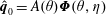 $\hat{\boldsymbol{q}}_{0}=A(\unicode[STIX]{x1D703})\unicode[STIX]{x1D731}(\unicode[STIX]{x1D703},\unicode[STIX]{x1D702})$
.
$\hat{\boldsymbol{q}}_{0}=A(\unicode[STIX]{x1D703})\unicode[STIX]{x1D731}(\unicode[STIX]{x1D703},\unicode[STIX]{x1D702})$
.
4 Results of the stability analysis
Following (3.7), we interpret the perturbation system as having three control parameters
 $\mathit{Re}=\mathit{Re}_{s}^{1/2}$
(here preferred to facilitate the comparison with the literature on the rotating disk and sphere),
$\mathit{Re}=\mathit{Re}_{s}^{1/2}$
(here preferred to facilitate the comparison with the literature on the rotating disk and sphere),
 $\bar{n}=n/\unicode[STIX]{x1D716}$
and
$\bar{n}=n/\unicode[STIX]{x1D716}$
and
 $\unicode[STIX]{x1D714}$
. Each parameter triple can be interrogated to determine its stability characteristics. We follow Garrett & Peake (Reference Garrett and Peake2002) by insisting that the disturbances rotate at some fixed multiple,
$\unicode[STIX]{x1D714}$
. Each parameter triple can be interrogated to determine its stability characteristics. We follow Garrett & Peake (Reference Garrett and Peake2002) by insisting that the disturbances rotate at some fixed multiple,
 $c$
, of the surface speed of the sphere at all latitudes in this fixed frame of reference. That is, we equate the disturbance phase velocity
$c$
, of the surface speed of the sphere at all latitudes in this fixed frame of reference. That is, we equate the disturbance phase velocity
 $\unicode[STIX]{x1D714}/n$
to
$\unicode[STIX]{x1D714}/n$
to
 $c\sin \unicode[STIX]{x1D703}$
. This then defines
$c\sin \unicode[STIX]{x1D703}$
. This then defines
 $\unicode[STIX]{x1D714}$
in terms of
$\unicode[STIX]{x1D714}$
in terms of
 $\bar{n}$
, leading to the new parameter triple
$\bar{n}$
, leading to the new parameter triple
 $(\mathit{Re},\bar{n},c)$
. Recall that
$(\mathit{Re},\bar{n},c)$
. Recall that
 $\mathit{Re}$
can be interpreted as the spin rate of the sphere while
$\mathit{Re}$
can be interpreted as the spin rate of the sphere while
 $\bar{n}$
is the azimuthal mode number of the disturbance under investigation (i.e. the number of vortices around the azimuth) and is necessarily an integer.
$\bar{n}$
is the azimuthal mode number of the disturbance under investigation (i.e. the number of vortices around the azimuth) and is necessarily an integer.
We proceed to consider the local stability properties of the flow incorporating non-parallel effects (i.e. without spatial homogenisation). The results of this analysis are associated with the appearance of spiral vortices within the boundary layer and can be related to the prior study of Garrett & Peake (Reference Garrett and Peake2002). We will discuss comparisons between our new results and those prior results as appropriate. However, when making such comparisons, it is important to note two significant distinctions: we now account for non-parallel effects, and our basic flow now allows for a better account of the boundary-layer eruption at the equator and also all
 $1/\mathit{Re}$
effects that were previously neglected. Unless otherwise stated, it should be assumed that all results are reported with both new aspects considered. Where necessary, we will occasionally report results from the non-parallel analysis performed on the previous steady flows (i.e. without the eruption and
$1/\mathit{Re}$
effects that were previously neglected. Unless otherwise stated, it should be assumed that all results are reported with both new aspects considered. Where necessary, we will occasionally report results from the non-parallel analysis performed on the previous steady flows (i.e. without the eruption and
 $1/\mathit{Re}$
effects), henceforth referred to as the Banks profiles (Banks Reference Banks1965).
$1/\mathit{Re}$
effects), henceforth referred to as the Banks profiles (Banks Reference Banks1965).
The growth rate of disturbances in the previous parallel-flow analysis (i.e. with spatial homogenisation) of Garrett & Peake (Reference Garrett and Peake2002) was given by
 $-\unicode[STIX]{x1D6FC}_{i}$
and their strictly local analysis required the stability to be determined separately at each latitude
$-\unicode[STIX]{x1D6FC}_{i}$
and their strictly local analysis required the stability to be determined separately at each latitude
 $\unicode[STIX]{x1D703}$
. In contrast, here we will determine the stability properties over the entire flow field in each calculation. Furthermore, the allowance for non-parallel effects now means that the growth rate of disturbances is given by
$\unicode[STIX]{x1D703}$
. In contrast, here we will determine the stability properties over the entire flow field in each calculation. Furthermore, the allowance for non-parallel effects now means that the growth rate of disturbances is given by
 $$\begin{eqnarray}\unicode[STIX]{x1D70E}=-\unicode[STIX]{x1D6FC}_{i}+\frac{\unicode[STIX]{x2202}}{\unicode[STIX]{x2202}\unicode[STIX]{x1D703}}\ln \sqrt{E},\end{eqnarray}$$
where
 $E$
is the disturbance kinetic energy given by
$E$
is the disturbance kinetic energy given by
 $$\begin{eqnarray}E=\int _{0}^{\infty }(|\hat{u} |^{2}+|\hat{u} |^{2}+|\hat{u} |^{2})\,\text{d}\unicode[STIX]{x1D702}.\end{eqnarray}$$
As will be discussed in § 5, the perturbation velocities account for
 $A(\unicode[STIX]{x1D703})$
, the correction for spatial inhomogeneity in
$A(\unicode[STIX]{x1D703})$
, the correction for spatial inhomogeneity in
 $\unicode[STIX]{x1D703}$
. The term
$\unicode[STIX]{x1D703}$
. The term
 $\unicode[STIX]{x2202}\ln \sqrt{E}/\unicode[STIX]{x2202}\unicode[STIX]{x1D703}$
is henceforth referred to as the non-parallel correction. In order to focus on the boundary layer, rather than the erupting jet at the equator, the stability results are only considered over the latitudinal domain between the pole and
$\unicode[STIX]{x2202}\ln \sqrt{E}/\unicode[STIX]{x2202}\unicode[STIX]{x1D703}$
is henceforth referred to as the non-parallel correction. In order to focus on the boundary layer, rather than the erupting jet at the equator, the stability results are only considered over the latitudinal domain between the pole and
 $\unicode[STIX]{x1D703}=80^{\circ }$
.
$\unicode[STIX]{x1D703}=80^{\circ }$
.
The perturbation system derived in § 3 is found to permit a number of distinct eigenmodes at each parameter triple
 $(Re,\bar{n},c)$
. This is illustrated in figure 12 for the particular case with
$(Re,\bar{n},c)$
. This is illustrated in figure 12 for the particular case with
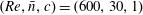 $(\mathit{Re},\bar{n},c)=(600,30,1)$
. Further investigation across the entire parameter space reveals that only a small number of these modes are physical (as evidenced by the form of the eigenfunctions, see § 5) and only two can lead to instability. The appearance of two unstable modes is consistent with Garrett & Peake (Reference Garrett and Peake2002) on the rotating sphere and indeed with the broader literature on the rotating-disk system (Hall Reference Hall1986; Malik Reference Malik1986; Lingwood Reference Lingwood1995). As will be discussed in the following sections, the mode denoted type I in the figure is found to be unstable over a much larger parameter space and is deemed equivalent to Garrett & Peake’s type I mode. The type I mode is known to arise from inviscid cross-flow effects and leads to the vortices observed in experiments. It is also related to the appearance of a local absolute instability. The type II mode is known to arise from viscous effects and is found to be unstable within a relatively limited parameter space. The type II mode is of theoretical rather than practical interest and we will focus on the type I mode in what follows. The type II mode is however considered separately in §§ 4.2 and 5.2.
$(\mathit{Re},\bar{n},c)=(600,30,1)$
. Further investigation across the entire parameter space reveals that only a small number of these modes are physical (as evidenced by the form of the eigenfunctions, see § 5) and only two can lead to instability. The appearance of two unstable modes is consistent with Garrett & Peake (Reference Garrett and Peake2002) on the rotating sphere and indeed with the broader literature on the rotating-disk system (Hall Reference Hall1986; Malik Reference Malik1986; Lingwood Reference Lingwood1995). As will be discussed in the following sections, the mode denoted type I in the figure is found to be unstable over a much larger parameter space and is deemed equivalent to Garrett & Peake’s type I mode. The type I mode is known to arise from inviscid cross-flow effects and leads to the vortices observed in experiments. It is also related to the appearance of a local absolute instability. The type II mode is known to arise from viscous effects and is found to be unstable within a relatively limited parameter space. The type II mode is of theoretical rather than practical interest and we will focus on the type I mode in what follows. The type II mode is however considered separately in §§ 4.2 and 5.2.

Figure 12. Eigenvalues’ evolution at
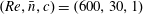 $(\mathit{Re},\bar{n},c)=(600,30,1)$
. Crosses indicate the eigenvalues at
$(\mathit{Re},\bar{n},c)=(600,30,1)$
. Crosses indicate the eigenvalues at
 $\unicode[STIX]{x1D703}=1^{\circ }$
and the circles show their evolution as
$\unicode[STIX]{x1D703}=1^{\circ }$
and the circles show their evolution as
 $\unicode[STIX]{x1D703}$
steps towards the equator in unit increments (right to left).
$\unicode[STIX]{x1D703}$
steps towards the equator in unit increments (right to left).
4.1 The type I mode
4.1.1 Stationary disturbances
We begin with the study of type I stationary disturbances, that is, disturbances that rotate with the local surface of the sphere, and fix
 $c=1$
. This results in the parameter pair
$c=1$
. This results in the parameter pair
 $(Re,\bar{n})$
giving the sphere spin rate and mode number of interest, respectively. Experiments (Sawatzki Reference Sawatzki1970; Kohama & Kobayashi Reference Kohama and Kobayashi1983) report the appearance of such stationary vortices on all but highly polished surfaces and this is an appropriate assumption to base the majority of our analysis. Non-stationary modes (namely with
$(Re,\bar{n})$
giving the sphere spin rate and mode number of interest, respectively. Experiments (Sawatzki Reference Sawatzki1970; Kohama & Kobayashi Reference Kohama and Kobayashi1983) report the appearance of such stationary vortices on all but highly polished surfaces and this is an appropriate assumption to base the majority of our analysis. Non-stationary modes (namely with
 $c\neq 1$
) are considered in § 4.1.2.
$c\neq 1$
) are considered in § 4.1.2.

Figure 13. Local growth rates at various
 $\mathit{Re}$
and
$\mathit{Re}$
and
 $\bar{n}$
; non-parallel growth (
$\bar{n}$
; non-parallel growth (
 $\unicode[STIX]{x1D70E}$
, ——) and parallel growth (
$\unicode[STIX]{x1D70E}$
, ——) and parallel growth (
 $-\unicode[STIX]{x1D6FC}_{i}$
,
$-\unicode[STIX]{x1D6FC}_{i}$
,
 $\times$
). Circles indicate neutral
$\times$
). Circles indicate neutral
 $\unicode[STIX]{x1D70E}$
.
$\unicode[STIX]{x1D70E}$
.
Figure 13 shows the parallel growth rate,
 $\unicode[STIX]{x1D70E}$
, at
$\unicode[STIX]{x1D70E}$
, at
 $\mathit{Re}=160$
and
$\mathit{Re}=160$
and
 $\mathit{Re}=700$
as a function of latitude with and without the non-parallel correction for various values of
$\mathit{Re}=700$
as a function of latitude with and without the non-parallel correction for various values of
 $\bar{n}$
. The results for
$\bar{n}$
. The results for
 $\mathit{Re}=160$
show a significant discrepancy arising from the parallel and non-parallel-flow assumptions. This is in contrast to
$\mathit{Re}=160$
show a significant discrepancy arising from the parallel and non-parallel-flow assumptions. This is in contrast to
 $\mathit{Re}=700$
where the non-parallel correction is seen to be relatively small, particularly for larger
$\mathit{Re}=700$
where the non-parallel correction is seen to be relatively small, particularly for larger
 $\bar{n}$
. These observations are consistent with Garrett & Peake’s assertion that the non-parallel correction reduces with increasing
$\bar{n}$
. These observations are consistent with Garrett & Peake’s assertion that the non-parallel correction reduces with increasing
 $\mathit{Re}$
.
$\mathit{Re}$
.
In each figure the appearance of neutral growth,
 $\unicode[STIX]{x1D70E}=0$
, is indicated with a circle. This can be interpreted as the latitudinal location of the onset of the type I instability for the particular mode number,
$\unicode[STIX]{x1D70E}=0$
, is indicated with a circle. This can be interpreted as the latitudinal location of the onset of the type I instability for the particular mode number,
 $\bar{n}$
, at spin rate
$\bar{n}$
, at spin rate
 $\mathit{Re}$
. At
$\mathit{Re}$
. At
 $\mathit{Re}=160$
we see that the
$\mathit{Re}=160$
we see that the
 $\bar{n}=9$
mode leads to a small pocket of instability at latitude
$\bar{n}=9$
mode leads to a small pocket of instability at latitude
 $\unicode[STIX]{x1D703}=74^{\circ }$
. The other mode numbers shown at this Reynolds number are seen to be stable and it is clear that
$\unicode[STIX]{x1D703}=74^{\circ }$
. The other mode numbers shown at this Reynolds number are seen to be stable and it is clear that
 $\mathit{Re}=160$
is close to the critical Reynolds number for onset of type I instability over the sphere. In contrast, at
$\mathit{Re}=160$
is close to the critical Reynolds number for onset of type I instability over the sphere. In contrast, at
 $\mathit{Re}=700$
all three mode numbers illustrated are unstable. In particular, the mode with
$\mathit{Re}=700$
all three mode numbers illustrated are unstable. In particular, the mode with
 $\bar{n}=20$
is unstable beyond
$\bar{n}=20$
is unstable beyond
 $\unicode[STIX]{x1D703}=22^{\circ }$
;
$\unicode[STIX]{x1D703}=22^{\circ }$
;
 $\bar{n}=40$
beyond
$\bar{n}=40$
beyond
 $\unicode[STIX]{x1D703}=30^{\circ }$
; and
$\unicode[STIX]{x1D703}=30^{\circ }$
; and
 $\bar{n}=60$
beyond
$\bar{n}=60$
beyond
 $\unicode[STIX]{x1D703}=43^{\circ }$
.
$\unicode[STIX]{x1D703}=43^{\circ }$
.
Such sampling of the stability of the flow can be performed at each parameter pair
 $(\mathit{Re},\bar{n})$
and this approach can be used to generate a single neutral curve for stationary type I modes across the entire system. Figure 14 shows this neutral curve in the
$(\mathit{Re},\bar{n})$
and this approach can be used to generate a single neutral curve for stationary type I modes across the entire system. Figure 14 shows this neutral curve in the
 $\mathit{Re}^{2}$
–
$\mathit{Re}^{2}$
–
 $\bar{n}$
plane. (Note that neutral curves are presented in terms of the spin Reynolds number,
$\bar{n}$
plane. (Note that neutral curves are presented in terms of the spin Reynolds number,
 $\mathit{Re}_{s}=\mathit{Re}^{2}$
which is typically used to report experimental data and its use here permits direct comparisons between our predictions and published experimental measurements.) Here the squares indicate neutrally unstable parameter pairs and a cross indicates the most amplified mode at each
$\mathit{Re}_{s}=\mathit{Re}^{2}$
which is typically used to report experimental data and its use here permits direct comparisons between our predictions and published experimental measurements.) Here the squares indicate neutrally unstable parameter pairs and a cross indicates the most amplified mode at each
 $\mathit{Re}$
. The resulting neutral curve is single lobed and shows a critical Reynolds number of
$\mathit{Re}$
. The resulting neutral curve is single lobed and shows a critical Reynolds number of
 $Re_{c,I}=159$
, below which no type I modes are predicted to be unstable. Note that
$Re_{c,I}=159$
, below which no type I modes are predicted to be unstable. Note that
 $Re_{c,I}$
is achieved for
$Re_{c,I}$
is achieved for
 $\bar{n}=10$
. Furthermore, the dotted line with circles shows experimental observations as reported by Kohama & Kobayashi (Reference Kohama and Kobayashi1983) for a sphere with diameter
$\bar{n}=10$
. Furthermore, the dotted line with circles shows experimental observations as reported by Kohama & Kobayashi (Reference Kohama and Kobayashi1983) for a sphere with diameter
 $D=250$
mm. We see remarkable agreement between these experimental observations and the predicted maximum amplified mode at each
$D=250$
mm. We see remarkable agreement between these experimental observations and the predicted maximum amplified mode at each
 $\mathit{Re}$
.
$\mathit{Re}$
.

Figure 14. Comparison of the neutral curve for the stationary type I mode (solid line with squares) in the
 $\mathit{Re}_{s}$
–
$\mathit{Re}_{s}$
–
 $\bar{n}$
plane with the experimental data of Kohama & Kobayashi (Reference Kohama and Kobayashi1983) for
$\bar{n}$
plane with the experimental data of Kohama & Kobayashi (Reference Kohama and Kobayashi1983) for
 $D=250$
mm (dotted line with circles). Crosses denote the mode number with the maximum amplification at each
$D=250$
mm (dotted line with circles). Crosses denote the mode number with the maximum amplification at each
 $\mathit{Re}$
.
$\mathit{Re}$
.
Figure 15 presents the same unstable points given in figure 14 but in terms of the
 $\mathit{Re}^{2}$
–
$\mathit{Re}^{2}$
–
 $\unicode[STIX]{x1D703}$
plane. In this context
$\unicode[STIX]{x1D703}$
plane. In this context
 $\unicode[STIX]{x1D703}$
is the location of the appearance of neutral stability, that is, locations analogous to those shown with circles in figure 13. Four independent experimental data sets are available in this form, each from different sized spheres (Sawatzki Reference Sawatzki1970; Kohama & Kobayashi Reference Kohama and Kobayashi1983), and these are also shown in the figure. The experimental comparisons with the most amplified mode numbers are less remarkable than in figure 14. However, we do note that, with the exception of Kohama & Kobayashi’s outlying results for the very small sphere (diameter
$\unicode[STIX]{x1D703}$
is the location of the appearance of neutral stability, that is, locations analogous to those shown with circles in figure 13. Four independent experimental data sets are available in this form, each from different sized spheres (Sawatzki Reference Sawatzki1970; Kohama & Kobayashi Reference Kohama and Kobayashi1983), and these are also shown in the figure. The experimental comparisons with the most amplified mode numbers are less remarkable than in figure 14. However, we do note that, with the exception of Kohama & Kobayashi’s outlying results for the very small sphere (diameter
 $D=70$
mm), each experimental data set falls within our predicted region of instability.
$D=70$
mm), each experimental data set falls within our predicted region of instability.

Figure 15. Comparisons of the neutral curve for the stationary type I mode (solid line with squares) in the
 $\mathit{Re}_{s}$
–
$\mathit{Re}_{s}$
–
 $\unicode[STIX]{x1D703}$
plane with experimental data of Kohama & Kobayashi (Reference Kohama and Kobayashi1983)
$\unicode[STIX]{x1D703}$
plane with experimental data of Kohama & Kobayashi (Reference Kohama and Kobayashi1983)
 $D=70$
mm (dotted line with crosses);
$D=70$
mm (dotted line with crosses);
 $D=150$
mm (dotted line with triangles);
$D=150$
mm (dotted line with triangles);
 $D=250$
mm (dotted line with circles); and Sawatzki (Reference Sawatzki1970),
$D=250$
mm (dotted line with circles); and Sawatzki (Reference Sawatzki1970),
 $D=240$
mm (dotted line with diamonds). Isolated crosses denote the latitude at the onset of the most amplified mode at each
$D=240$
mm (dotted line with diamonds). Isolated crosses denote the latitude at the onset of the most amplified mode at each
 $\mathit{Re}$
.
$\mathit{Re}$
.
4.1.2 Travelling disturbances
By varying the value of
 $c$
we are able to consider type I disturbances that are moving relative to the sphere surface. The case that
$c$
we are able to consider type I disturbances that are moving relative to the sphere surface. The case that
 $c>1$
denotes disturbances travelling more quickly than the local surface speed, and
$c>1$
denotes disturbances travelling more quickly than the local surface speed, and
 $c<1$
denotes disturbances travelling more slowly. For example,
$c<1$
denotes disturbances travelling more slowly. For example,
 $c=1.1$
and
$c=1.1$
and
 $c=0.9$
would correspond to disturbances travelling at 110 % and 90 % of the local surface speed, respectively. In practice, travelling vortices are difficult to observe in experiments unless great care is taken to avoid the appearance of any surface roughness (that would otherwise fix the vortex pattern relative to the rotating surface) and the boundary-layer excitation results instead from free-stream turbulence. However, in theory, travelling modes can be even more dangerous than stationary modes (in the sense of lower critical
$c=0.9$
would correspond to disturbances travelling at 110 % and 90 % of the local surface speed, respectively. In practice, travelling vortices are difficult to observe in experiments unless great care is taken to avoid the appearance of any surface roughness (that would otherwise fix the vortex pattern relative to the rotating surface) and the boundary-layer excitation results instead from free-stream turbulence. However, in theory, travelling modes can be even more dangerous than stationary modes (in the sense of lower critical
 $\mathit{Re}$
) and are also known to play a role in local absolute instability (see, for example, the work of Lingwood Reference Lingwood1995; Corke & Knasiak Reference Corke and Knasiak1998; Othman & Corke Reference Othman and Corke2006; Corke, Matlis & Othman Reference Corke, Matlis and Othman2007, on the related rotating-disk system).
$\mathit{Re}$
) and are also known to play a role in local absolute instability (see, for example, the work of Lingwood Reference Lingwood1995; Corke & Knasiak Reference Corke and Knasiak1998; Othman & Corke Reference Othman and Corke2006; Corke, Matlis & Othman Reference Corke, Matlis and Othman2007, on the related rotating-disk system).
The approach taken in § 4.1.1 has been repeated for various
 $c$
and table 1 gives the resulting mode number for the lowest critical
$c$
and table 1 gives the resulting mode number for the lowest critical
 $\mathit{Re}$
in each case. We see that slowly travelling modes are predicted to be less dangerous (i.e. increased
$\mathit{Re}$
in each case. We see that slowly travelling modes are predicted to be less dangerous (i.e. increased
 $Re_{c}$
) with reduced
$Re_{c}$
) with reduced
 $c$
. In contrast, quickly travelling modes are predicted to be more dangerous with increased
$c$
. In contrast, quickly travelling modes are predicted to be more dangerous with increased
 $c$
. Note however that the corresponding mode number reduces to small values that are unphysical in practice – certainly the experimental observations of Sawatzki (Reference Sawatzki1970) and Kohama & Kobayashi (Reference Kohama and Kobayashi1983) never report fewer than ten vortices.
$c$
. Note however that the corresponding mode number reduces to small values that are unphysical in practice – certainly the experimental observations of Sawatzki (Reference Sawatzki1970) and Kohama & Kobayashi (Reference Kohama and Kobayashi1983) never report fewer than ten vortices.
Figure 16 shows the evolution of the maximum amplification rate,
 $\unicode[STIX]{x1D70E}_{max}$
, of each travelling type I mode as
$\unicode[STIX]{x1D70E}_{max}$
, of each travelling type I mode as
 $\mathit{Re}$
is increased into the locally unstable regime. Amplification rates for very slowly travelling modes, that is with
$\mathit{Re}$
is increased into the locally unstable regime. Amplification rates for very slowly travelling modes, that is with
 $c\leqslant 0.7$
, are found to be significantly lower than the more rapidly travelling modes for moderate
$c\leqslant 0.7$
, are found to be significantly lower than the more rapidly travelling modes for moderate
 $\mathit{Re}$
. The figure suggests that stationary and quickly travelling modes dominate for
$\mathit{Re}$
. The figure suggests that stationary and quickly travelling modes dominate for
 $\mathit{Re}<400$
. However, despite the mode with
$\mathit{Re}<400$
. However, despite the mode with
 $c=0.8$
having a later onset, it is the most amplified by some margin for
$c=0.8$
having a later onset, it is the most amplified by some margin for
 $\mathit{Re}>400$
. We note that these observations are consistent with Garrett (Reference Garrett2010) who found that the type I mode with
$\mathit{Re}>400$
. We note that these observations are consistent with Garrett (Reference Garrett2010) who found that the type I mode with
 $c=0.75$
has the greatest amplification rate under the parallel-flow assumption. There he associates this result with the single experimental observation by Kobayashi & Arai (Reference Kobayashi, Arai, Arnal and Michel1990) of vortices travelling at 76 % of the local surface speed of the sphere rotating in otherwise still fluid. Unfortunately no further information is given by Kobayashi & Arai and further comparisons with our new theoretical prediction cannot be made.
$c=0.75$
has the greatest amplification rate under the parallel-flow assumption. There he associates this result with the single experimental observation by Kobayashi & Arai (Reference Kobayashi, Arai, Arnal and Michel1990) of vortices travelling at 76 % of the local surface speed of the sphere rotating in otherwise still fluid. Unfortunately no further information is given by Kobayashi & Arai and further comparisons with our new theoretical prediction cannot be made.

Figure 16. Evolution of
 $\unicode[STIX]{x1D70E}_{max}$
for
$\unicode[STIX]{x1D70E}_{max}$
for
 $c=0.8$
(dashed line), 1 (solid line), 1.2 (dash-dot line), 1.4 (dotted line) and 0.7 (line with circles).
$c=0.8$
(dashed line), 1 (solid line), 1.2 (dash-dot line), 1.4 (dotted line) and 0.7 (line with circles).
Table 1. The critical
 $\mathit{Re}$
and associated mode number for the onset of travelling disturbances at various
$\mathit{Re}$
and associated mode number for the onset of travelling disturbances at various
 $c$
.
$c$
.
4.2 Stationary type II modes and the full non-parallel neutral curve
As illustrated in figure 12, our analysis leads to the prediction of an additional instability mechanism that we have associated with the type II mode identified by the parallel-flow study of Garrett & Peake (Reference Garrett and Peake2002). Although there is no experimental evidence for the type II mode in the literature for the rotating sphere or related boundary-layer flows, predictions of its theoretical existence provide an additional means by which to compare across analytical studies. Figure 17 illustrates the non-parallel growth rates of this mode at
 $\mathit{Re}=50$
for increasing
$\mathit{Re}=50$
for increasing
 $\bar{n}$
and pockets of instability can be seen clearly for
$\bar{n}$
and pockets of instability can be seen clearly for
 $\bar{n}=1$
and 2.
$\bar{n}=1$
and 2.

Figure 17. Growth rates
 $\unicode[STIX]{x1D70E}$
for stationary type II modes at
$\unicode[STIX]{x1D70E}$
for stationary type II modes at
 $\mathit{Re}=50$
for
$\mathit{Re}=50$
for
 $\bar{n}=1$
(——), 2 (– – –), 3 (– - –) and 4 (
$\bar{n}=1$
(——), 2 (– – –), 3 (– - –) and 4 (
Following the process discussed in § 4.1.1, it is possible to examine the stability of the type II mode at each parameter triple
 $(\mathit{Re},\bar{n},c)$
and generate a neutral curve for this mode. This has been done for stationary disturbances (
$(\mathit{Re},\bar{n},c)$
and generate a neutral curve for this mode. This has been done for stationary disturbances (
 $c=1$
) and the full neutral curve arising from the types I and II modes is shown in the
$c=1$
) and the full neutral curve arising from the types I and II modes is shown in the
 $\mathit{Re}$
–
$\mathit{Re}$
–
 $\bar{n}$
plane in figure 18. Note that the familiar two-lobed structure is recovered. That is, the type II mode has led to an additional lobe in the neutral curve characterised by small
$\bar{n}$
plane in figure 18. Note that the familiar two-lobed structure is recovered. That is, the type II mode has led to an additional lobe in the neutral curve characterised by small
 $\bar{n}$
that is seen to be unstable at all
$\bar{n}$
that is seen to be unstable at all
 $\mathit{Re}$
above a critical value of
$\mathit{Re}$
above a critical value of
 $Re_{c,II}=41$
. The critical Reynolds number for the onset of the type II mode is therefore considerably lower than that for the type I mode computed as
$Re_{c,II}=41$
. The critical Reynolds number for the onset of the type II mode is therefore considerably lower than that for the type I mode computed as
 $Re_{c,I}=159$
in § 4.1.1.
$Re_{c,I}=159$
in § 4.1.1.
Figure 18. The full neutral curve for stationary (
 $c=1$
) type I (▫) and type II (▵) modes. The dotted lines are the strictly local neutral curves due to Garrett & Peake (Reference Garrett and Peake2002) at
$c=1$
) type I (▫) and type II (▵) modes. The dotted lines are the strictly local neutral curves due to Garrett & Peake (Reference Garrett and Peake2002) at
 $\unicode[STIX]{x1D703}=30^{\circ }$
–
$\unicode[STIX]{x1D703}=30^{\circ }$
–
 $80^{\circ }$
in ten degree increments (right to left).
$80^{\circ }$
in ten degree increments (right to left).
The strictly local analysis of Garrett & Peake (Reference Garrett and Peake2002) generates a different neutral curve at each latitudinal position. Our single neutral curve for the entire flow field should therefore be compared to the envelope of all neutral curves generated by Garrett & Peake and this comparison is shown in figure 18. The comparison shows broad qualitative agreement, however there are some quantitative differences between the two studies. The most significant being around the predicted critical Reynolds numbers of each mode and along the upper branch of the type I lobe. Garrett & Peake report that their type II mode dominates for latitudes above
 $\unicode[STIX]{x1D703}=66^{\circ }$
and so the comparison of the type I unstable points is relevant for all but the two leftmost curves in figure 18 (where
$\unicode[STIX]{x1D703}=66^{\circ }$
and so the comparison of the type I unstable points is relevant for all but the two leftmost curves in figure 18 (where
 $\unicode[STIX]{x1D703}=70^{\circ }$
and
$\unicode[STIX]{x1D703}=70^{\circ }$
and
 $80^{\circ }$
). With this is mind we see good agreement between the critical Reynolds numbers for the onset of their type I mode, elsewhere reported to be
$80^{\circ }$
). With this is mind we see good agreement between the critical Reynolds numbers for the onset of their type I mode, elsewhere reported to be
 $\mathit{Re}=155$
(Garrett Reference Garrett2002), and our
$\mathit{Re}=155$
(Garrett Reference Garrett2002), and our
 $Re_{c,I}=159$
. (Note that figure 18 does not show Garrett & Peake’s parallel-flow results at
$Re_{c,I}=159$
. (Note that figure 18 does not show Garrett & Peake’s parallel-flow results at
 $\unicode[STIX]{x1D703}=66^{\circ }$
, only at
$\unicode[STIX]{x1D703}=66^{\circ }$
, only at
 $\unicode[STIX]{x1D703}=60^{\circ }$
and
$\unicode[STIX]{x1D703}=60^{\circ }$
and
 $70^{\circ }$
.) In terms of the type II mode, Garrett & Peake report a critical Reynolds number of around
$70^{\circ }$
.) In terms of the type II mode, Garrett & Peake report a critical Reynolds number of around
 $\mathit{Re}=14$
for the neutral curve at
$\mathit{Re}=14$
for the neutral curve at
 $\unicode[STIX]{x1D703}=80^{\circ }$
. This compares poorly with our critical value of
$\unicode[STIX]{x1D703}=80^{\circ }$
. This compares poorly with our critical value of
 $Re_{c,II}=41$
. However, as discussed in § 4.1, discrepancies at these very low Reynolds numbers are likely to be due to the parallel-flow assumption used by Garrett & Peake which is now known to be significant at low
$Re_{c,II}=41$
. However, as discussed in § 4.1, discrepancies at these very low Reynolds numbers are likely to be due to the parallel-flow assumption used by Garrett & Peake which is now known to be significant at low
 $\mathit{Re}$
, in addition to the fact that their base flow was different.
$\mathit{Re}$
, in addition to the fact that their base flow was different.
Although not shown here, the neutral curve resulting from our non-parallel analysis of the Banks flow profiles shows very good agreement with Garrett & Peake along the upper neutral curve. We therefore attribute the difference along the upper branch to the allowance for the boundary-layer eruption and other
 $1/\mathit{Re}$
effects in this new analysis. It is interesting to note that the close agreement shown between theory and experiment in figure 14 is lost when using the Banks profiles; in particular, the number of vortices is then consistently under-predicted when compared to experimental data.
$1/\mathit{Re}$
effects in this new analysis. It is interesting to note that the close agreement shown between theory and experiment in figure 14 is lost when using the Banks profiles; in particular, the number of vortices is then consistently under-predicted when compared to experimental data.
5 Eigenfunctions
We now turn to a discussion of the eigenfunctions of the system. In particular, we focus on the azimuthal perturbation velocities, i.e.
 $\hat{\unicode[STIX]{x1D719}}(\unicode[STIX]{x1D702},\unicode[STIX]{x1D703})=\hat{v}(\unicode[STIX]{x1D702},\unicode[STIX]{x1D703})$
in the notation of (3.7). Note that our choice of the azimuthal perturbation component is arbitrary and any perturbation component (velocity or pressure) could be used.
$\hat{\unicode[STIX]{x1D719}}(\unicode[STIX]{x1D702},\unicode[STIX]{x1D703})=\hat{v}(\unicode[STIX]{x1D702},\unicode[STIX]{x1D703})$
in the notation of (3.7). Note that our choice of the azimuthal perturbation component is arbitrary and any perturbation component (velocity or pressure) could be used.
Within our formulation the parallel-flow eigenfunction,
 $\bar{v}(\unicode[STIX]{x1D702},\unicode[STIX]{x1D703})$
, is computed together with its non-parallel correction,
$\bar{v}(\unicode[STIX]{x1D702},\unicode[STIX]{x1D703})$
, is computed together with its non-parallel correction,
 $A(\unicode[STIX]{x1D703})$
, and then combined to obtain the non-parallel eigenfunction at each parameter triple
$A(\unicode[STIX]{x1D703})$
, and then combined to obtain the non-parallel eigenfunction at each parameter triple
 $(\mathit{Re},\bar{n},c)$
,
$(\mathit{Re},\bar{n},c)$
,
 $$\begin{eqnarray}\hat{v}(\unicode[STIX]{x1D702},\unicode[STIX]{x1D703})=\bar{v}(\unicode[STIX]{x1D702},\unicode[STIX]{x1D703})A(\unicode[STIX]{x1D703}).\end{eqnarray}$$
Consistent with Cooper et al. (Reference Cooper, Harris, Garrett, Özkan and Thomas2015) and others in the literature we report the absolute value of the complex eigenfunctions in what follows.
As previously discussed, many of the additional modes identified in figure 12 can be dismissed as numerical artefacts and these are identified by the unphysical shape of their parallel eigenfunction,
 $\bar{v}(\unicode[STIX]{x1D702},\unicode[STIX]{x1D703})$
, sampled at some
$\bar{v}(\unicode[STIX]{x1D702},\unicode[STIX]{x1D703})$
, sampled at some
 $\unicode[STIX]{x1D703}$
. Example parallel type I and II eigenmodes are illustrated in figure 19.
$\unicode[STIX]{x1D703}$
. Example parallel type I and II eigenmodes are illustrated in figure 19.

Figure 19. Physical eigenfunctions at
 $\unicode[STIX]{x1D703}=50^{\circ }$
. (a) Type I
$\unicode[STIX]{x1D703}=50^{\circ }$
. (a) Type I
 $|\bar{v}(\unicode[STIX]{x1D702},50)|$
for
$|\bar{v}(\unicode[STIX]{x1D702},50)|$
for
 $(\mathit{Re},\bar{n},c)=(600,30,1)$
, (b) Type II
$(\mathit{Re},\bar{n},c)=(600,30,1)$
, (b) Type II
 $|\bar{v}(\unicode[STIX]{x1D702},50)|$
for
$|\bar{v}(\unicode[STIX]{x1D702},50)|$
for
 $(\mathit{Re},\bar{n},c)=(100,4,1)$
. (Each is normalised by
$(\mathit{Re},\bar{n},c)=(100,4,1)$
. (Each is normalised by
 $\max |\bar{v}(\unicode[STIX]{x1D703},\unicode[STIX]{x1D702})|$
at the particular
$\max |\bar{v}(\unicode[STIX]{x1D703},\unicode[STIX]{x1D702})|$
at the particular
 $(\mathit{Re},\bar{n},c)$
.)
$(\mathit{Re},\bar{n},c)$
.)
5.1 Spatial evolution of the type I modes
The behaviour of the type I eigenfunction is found to be consistent across the entire parameter space and, by way of illustration, we present only the parameter triple
 $(\mathit{Re},\bar{n},c)=(600,30,1)$
. This particular parameter set is known to be unstable via the type I mode, as can be confirmed from figure 18. The parallel eigenfunction,
$(\mathit{Re},\bar{n},c)=(600,30,1)$
. This particular parameter set is known to be unstable via the type I mode, as can be confirmed from figure 18. The parallel eigenfunction,
 $\bar{v}(\unicode[STIX]{x1D703},\unicode[STIX]{x1D702})$
, is shown in figure 20(a) and that allowing for the non-parallel correction,
$\bar{v}(\unicode[STIX]{x1D703},\unicode[STIX]{x1D702})$
, is shown in figure 20(a) and that allowing for the non-parallel correction,
 $\hat{v}(\unicode[STIX]{x1D703},\unicode[STIX]{x1D702})$
, is shown in figure 20(b). The parallel eigenfunction shows that the type I mode exists at all latitudes over the sphere and tends to grow in its normal extent and magnitude as the disturbance moves from the pole towards the equator. The non-parallel correction is seen to be significant and suggests that an unstable type I mode would grow rapidly from even small latitudes.
$\hat{v}(\unicode[STIX]{x1D703},\unicode[STIX]{x1D702})$
, is shown in figure 20(b). The parallel eigenfunction shows that the type I mode exists at all latitudes over the sphere and tends to grow in its normal extent and magnitude as the disturbance moves from the pole towards the equator. The non-parallel correction is seen to be significant and suggests that an unstable type I mode would grow rapidly from even small latitudes.

Figure 20. The type I azimuthal perturbation velocity field for
 $(\mathit{Re},\bar{n},c)=(600,30,1)$
. (a) Parallel eigenfunction,
$(\mathit{Re},\bar{n},c)=(600,30,1)$
. (a) Parallel eigenfunction,
 $|\bar{v}(\unicode[STIX]{x1D703},\unicode[STIX]{x1D702})|$
, (b) non-parallel eigenfunction,
$|\bar{v}(\unicode[STIX]{x1D703},\unicode[STIX]{x1D702})|$
, (b) non-parallel eigenfunction,
 $|\hat{v}(\unicode[STIX]{x1D703},\unicode[STIX]{x1D702})|$
. (Each figure is normalised independently by its maximum value.)
$|\hat{v}(\unicode[STIX]{x1D703},\unicode[STIX]{x1D702})|$
. (Each figure is normalised independently by its maximum value.)
5.2 Spatial evolution of the type II modes
The parallel and non-parallel type II eigenfunctions are illustrated from figure 21 for
 $(\mathit{Re},\bar{c})=(100,4,1)$
. This particular mode is known to be unstable, as can be confirmed in figure 18. Consistent with the parallel type I mode in figure 20(a), the parallel type II mode is seen to exist at all latitudes, however its normal extent and magnitude are reasonably constant over
$(\mathit{Re},\bar{c})=(100,4,1)$
. This particular mode is known to be unstable, as can be confirmed in figure 18. Consistent with the parallel type I mode in figure 20(a), the parallel type II mode is seen to exist at all latitudes, however its normal extent and magnitude are reasonably constant over
 $\unicode[STIX]{x1D703}$
. Furthermore, in direct contrast to the type I mode, the non-parallel correction is seen to focus the importance of the type II mode to higher latitudes. The contrasting behaviour of the non-parallel types I and II modes is consistent with the conclusion of Garrett & Peake that an unstable type II mode is potentially important only at higher latitudes, by which point unstable type I modes would dominate the flow.
$\unicode[STIX]{x1D703}$
. Furthermore, in direct contrast to the type I mode, the non-parallel correction is seen to focus the importance of the type II mode to higher latitudes. The contrasting behaviour of the non-parallel types I and II modes is consistent with the conclusion of Garrett & Peake that an unstable type II mode is potentially important only at higher latitudes, by which point unstable type I modes would dominate the flow.
Note that each panel in figures 20 and 21 is normalised by its own maximum value and quantitative comparisons should not be made between any plots.

Figure 21. The type II azimuthal perturbation velocity field for
 $(\mathit{Re},\bar{n},c)=(100,4,1)$
. (a) Parallel eigenfunction,
$(\mathit{Re},\bar{n},c)=(100,4,1)$
. (a) Parallel eigenfunction,
 $|\bar{v}(\unicode[STIX]{x1D703},\unicode[STIX]{x1D702})|$
, (b) Non-parallel eigenfunction,
$|\bar{v}(\unicode[STIX]{x1D703},\unicode[STIX]{x1D702})|$
, (b) Non-parallel eigenfunction,
 $|\hat{v}(\unicode[STIX]{x1D703},\unicode[STIX]{x1D702})|$
. (Each figure is normalised independently by its maximum value.)
$|\hat{v}(\unicode[STIX]{x1D703},\unicode[STIX]{x1D702})|$
. (Each figure is normalised independently by its maximum value.)
6 Conclusion
We have considered the boundary-layer flow over the rotating sphere, both in terms of the computation of the steady flow and also its linear stability properties. The steady-flow solution has been improved significantly from the original formulation proposed by Howarth (Reference Howarth1951) and solved by Banks (Reference Banks1965). It now better accounts for the boundary-layer eruption at the equator (Calabretto et al. Reference Calabretto, Levy, Denier and Mattner2015) and also the inclusion of a number of viscous terms that were previously neglected in the Howarth and Banks solutions.
The linear stability of the flow was considered as a function of spin rate (Reynolds number) using a weakly non-parallel analysis, that is, without imposing a spatial homogenisation of the boundary layer. As expected from prior parallel-flow studies (i.e. with spatial homogenisation imposed), two instability modes were found to dictate the local properties of the flow. These are denoted as the type I and type II modes. A single neutral curve was computed for the entire flow field and each mode was evident as a distinct lobe. The type I mode is dominant and is associated with the experimentally observed spiral vortices in the boundary layer (Sawatzki Reference Sawatzki1970; Kohama & Kobayashi Reference Kohama and Kobayashi1983; Kobayashi & Arai Reference Kobayashi, Arai, Arnal and Michel1990). Stationary types I and II modes were found to have critical Reynolds numbers of
 $\mathit{Re}_{c,I}=159$
and
$\mathit{Re}_{c,I}=159$
and
 $\mathit{Re}_{c,II}=41$
, respectively. Remarkable agreement was found between the most amplified stationary type I mode number and the experimentally observed number of vortices (Kohama & Kobayashi Reference Kohama and Kobayashi1983) as a function of spin rate. Furthermore, experimental observations of the latitudinal location of the onset of spiral vortices fell within our predicted neutral curve. Travelling type I modes were also considered but are expected to correspond to the appearance of spiral vortices on only highly polished surfaces, where the boundary-layer excitation results from free-stream turbulence rather than surface roughness. In this case, type I modes travelling with speeds of 70 %–80 % of the local surface speed of the sphere were found to be the most amplified for sufficiently high spin rates. This is consistent with the experimental observation by Kobayashi & Arai (Reference Kobayashi, Arai, Arnal and Michel1990) of ‘slow’ vortices travelling at 76 % of the local sphere surface speed.
$\mathit{Re}_{c,II}=41$
, respectively. Remarkable agreement was found between the most amplified stationary type I mode number and the experimentally observed number of vortices (Kohama & Kobayashi Reference Kohama and Kobayashi1983) as a function of spin rate. Furthermore, experimental observations of the latitudinal location of the onset of spiral vortices fell within our predicted neutral curve. Travelling type I modes were also considered but are expected to correspond to the appearance of spiral vortices on only highly polished surfaces, where the boundary-layer excitation results from free-stream turbulence rather than surface roughness. In this case, type I modes travelling with speeds of 70 %–80 % of the local surface speed of the sphere were found to be the most amplified for sufficiently high spin rates. This is consistent with the experimental observation by Kobayashi & Arai (Reference Kobayashi, Arai, Arnal and Michel1990) of ‘slow’ vortices travelling at 76 % of the local sphere surface speed.
Parallel and non-parallel eigenmodes of both mode types have been computed for the first time. The spatial evolution of these suggests that, while the type I mode is important at all latitudes, the type II mode is potentially important at only larger latitudes, at which point unstable type I modes would already dominate the flow. This is a potential explanation for why type II modes have never been observed in experiments.
Our study extends those originally presented by Garrett & Peake (Reference Garrett and Peake2002) and Garrett (Reference Garrett2010), performed using the parallel-flow approximation and Banks steady-flow solutions. The non-parallel correction was found to be significant, particularly for low Reynolds numbers and small mode numbers.
Acknowledgements
S.J.G. is supported by a Senior Research Fellowship of the Royal Academy of Engineering, funded by the Leverhulme Trust. The hospitality of Dr S.O. Stephen and the wider Department of Mathematics, University of Sydney is acknowledged, where S.J.G. held a Visiting Professorship in 2016 and much of this paper was drafted. The continued hospitality of the Linné FLOW Centre, KTH is also acknowledged. J. Canton and Dr P. Schlatter are acknowledged for fruitful discussions and for some simulations that supported the present mean-flow analysis.
Appendix A. Double-deck description of the impinging region
This section replicates the main steps of the derivation proposed by Smith & Duck (Reference Smith and Duck1977) and extends it with the inclusion of the tangential velocity field. The derivation assumes a two-layer structure upstream of the separation point. In the upper layer the coordinates are scaled as
 $$\begin{eqnarray}\unicode[STIX]{x1D6FD}^{\prime }=\frac{\unicode[STIX]{x1D703}-\unicode[STIX]{x03C0}/2}{\unicode[STIX]{x1D716}^{6/7}},\quad \unicode[STIX]{x1D702}=\frac{r-1}{\unicode[STIX]{x1D716}}.\end{eqnarray}$$
The velocity components are then linearised as
 $$\begin{eqnarray}\displaystyle \left.\begin{array}{@{}c@{}}U=U_{0}\left({\displaystyle \frac{\unicode[STIX]{x03C0}}{2}},\unicode[STIX]{x1D702}\right)+\unicode[STIX]{x1D716}^{2/7}u_{1},\quad V=V_{0}\left({\displaystyle \frac{\unicode[STIX]{x03C0}}{2}},\unicode[STIX]{x1D702}\right)+\unicode[STIX]{x1D716}^{2/7}v_{1},\\ W=\unicode[STIX]{x1D716}^{3/7}w_{1},\quad p=\unicode[STIX]{x1D716}^{4/7}p_{1},\end{array}\right\} & & \displaystyle\end{eqnarray}$$
leading to the equations
 $$\begin{eqnarray}\displaystyle & \displaystyle \frac{\unicode[STIX]{x2202}u_{1}}{\unicode[STIX]{x2202}\unicode[STIX]{x1D6FD}^{\prime }}+\frac{\unicode[STIX]{x2202}w_{1}}{\unicode[STIX]{x2202}\unicode[STIX]{x1D702}}=0, & \displaystyle\end{eqnarray}$$
 $$\begin{eqnarray}\displaystyle & \displaystyle U_{0}\frac{\unicode[STIX]{x2202}u_{1}}{\unicode[STIX]{x2202}\unicode[STIX]{x1D6FD}^{\prime }}+w_{1}\frac{\unicode[STIX]{x2202}U_{0}}{\unicode[STIX]{x2202}\unicode[STIX]{x1D702}}=0, & \displaystyle\end{eqnarray}$$
 $$\begin{eqnarray}\displaystyle & \displaystyle U_{0}\frac{\unicode[STIX]{x2202}v_{1}}{\unicode[STIX]{x2202}\unicode[STIX]{x1D6FD}^{\prime }}+w_{1}\frac{\unicode[STIX]{x2202}V_{0}}{\unicode[STIX]{x2202}\unicode[STIX]{x1D702}}=0, & \displaystyle\end{eqnarray}$$
 $$\begin{eqnarray}\displaystyle & \displaystyle U_{0}\frac{\unicode[STIX]{x2202}w_{1}}{\unicode[STIX]{x2202}\unicode[STIX]{x1D6FD}^{\prime }}=-\frac{\unicode[STIX]{x2202}p}{\unicode[STIX]{x2202}\unicode[STIX]{x1D702}}, & \displaystyle\end{eqnarray}$$
with solution
 $$\begin{eqnarray}u_{1}=A(\unicode[STIX]{x1D6FD}^{\prime })\frac{\unicode[STIX]{x2202}U_{0}}{\unicode[STIX]{x2202}\unicode[STIX]{x1D702}},\quad v_{1}=A(\unicode[STIX]{x1D6FD}^{\prime })\frac{\unicode[STIX]{x2202}V_{0}}{\unicode[STIX]{x2202}\unicode[STIX]{x1D702}},\quad w_{1}=-A^{\prime }(\unicode[STIX]{x1D6FD}^{\prime })U_{0}\left(\frac{\unicode[STIX]{x03C0}}{2},\unicode[STIX]{x1D702}\right),\end{eqnarray}$$
 $$\begin{eqnarray}p_{1}=P_{w}(\unicode[STIX]{x1D6FD}^{\prime })+A^{\prime \prime }(\unicode[STIX]{x1D6FD}^{\prime })\int _{0}^{\unicode[STIX]{x1D702}}U_{0}^{2}\left(\frac{\unicode[STIX]{x03C0}}{2},\unicode[STIX]{x1D712}\right)\text{d}\unicode[STIX]{x1D712},\end{eqnarray}$$
for a certain unknown function
 $A(\unicode[STIX]{x1D6FD}^{\prime })$
.
$A(\unicode[STIX]{x1D6FD}^{\prime })$
.
 $A^{\prime }$
and
$A^{\prime }$
and
 $A^{\prime \prime }$
indicate the first and second derivative of the
$A^{\prime \prime }$
indicate the first and second derivative of the
 $A$
function. As a boundary condition,
$A$
function. As a boundary condition,
 $p_{1}\rightarrow 0$
as
$p_{1}\rightarrow 0$
as
 $\unicode[STIX]{x1D702}\rightarrow \infty$
leading to
$\unicode[STIX]{x1D702}\rightarrow \infty$
leading to
 $$\begin{eqnarray}P_{w}(\unicode[STIX]{x1D6FD}^{\prime })=-\frac{1}{\unicode[STIX]{x1D6FE}}A^{\prime \prime }(\unicode[STIX]{x1D6FD}^{\prime })\longrightarrow -\frac{\text{d}P_{w}}{\text{d}\unicode[STIX]{x1D6FD}^{\prime }}=\frac{1}{\unicode[STIX]{x1D6FE}}A^{\prime \prime \prime }(\unicode[STIX]{x1D6FD}^{\prime }),\end{eqnarray}$$
where
 $1/\unicode[STIX]{x1D6FE}=\int _{0}^{\infty }U_{0}^{2}(\unicode[STIX]{x03C0}/2,\unicode[STIX]{x1D712})\,\text{d}\unicode[STIX]{x1D712}=0.0583$
.
$1/\unicode[STIX]{x1D6FE}=\int _{0}^{\infty }U_{0}^{2}(\unicode[STIX]{x03C0}/2,\unicode[STIX]{x1D712})\,\text{d}\unicode[STIX]{x1D712}=0.0583$
.

Figure 22. (——)
 $-A/100$
, (– – –)
$-A/100$
, (– – –)
 $\unicode[STIX]{x2202}\tilde{U} /\unicode[STIX]{x2202}Z$
upstream of the separation point.
$\unicode[STIX]{x2202}\tilde{U} /\unicode[STIX]{x2202}Z$
upstream of the separation point.
Since
 $u_{1}\rightarrow \unicode[STIX]{x1D705}A$
as
$u_{1}\rightarrow \unicode[STIX]{x1D705}A$
as
 $\unicode[STIX]{x1D702}\rightarrow 0$
(with
$\unicode[STIX]{x1D702}\rightarrow 0$
(with
 $\unicode[STIX]{x1D705}$
indicating the first derivative of the
$\unicode[STIX]{x1D705}$
indicating the first derivative of the
 $U_{0}$
profile at
$U_{0}$
profile at
 $\unicode[STIX]{x1D702}=0$
), a lower deck is needed. This is defined by the stretched variables
$\unicode[STIX]{x1D702}=0$
), a lower deck is needed. This is defined by the stretched variables
 $Z=\unicode[STIX]{x1D716}^{-9/7}(r-1)=\unicode[STIX]{x1D716}^{-2/7}\unicode[STIX]{x1D702}$
, through the asymptotic expressions
$Z=\unicode[STIX]{x1D716}^{-9/7}(r-1)=\unicode[STIX]{x1D716}^{-2/7}\unicode[STIX]{x1D702}$
, through the asymptotic expressions
 $$\begin{eqnarray}U=\unicode[STIX]{x1D716}^{2/7}\tilde{U} ,\quad V=1+\unicode[STIX]{x1D716}^{2/7}\tilde{V},\quad W=\unicode[STIX]{x1D716}^{5/7}\tilde{W},\end{eqnarray}$$
and by the equations
 $$\begin{eqnarray}\displaystyle & \displaystyle \frac{\unicode[STIX]{x2202}\tilde{U} }{\unicode[STIX]{x2202}\unicode[STIX]{x1D6FD}^{\prime }}+\frac{\unicode[STIX]{x2202}\tilde{W}}{\unicode[STIX]{x2202}Z}=0, & \displaystyle\end{eqnarray}$$
 $$\begin{eqnarray}\displaystyle & \displaystyle \tilde{U} \frac{\unicode[STIX]{x2202}\tilde{U} }{\unicode[STIX]{x2202}\unicode[STIX]{x1D6FD}^{\prime }}+\tilde{W}\frac{\unicode[STIX]{x2202}\tilde{U} }{\unicode[STIX]{x2202}\unicode[STIX]{x1D702}}=-\frac{\text{d}P_{w}}{\text{d}\unicode[STIX]{x1D6FD}^{\prime }}+\frac{\unicode[STIX]{x2202}^{2}\tilde{U} }{\unicode[STIX]{x2202}Z^{2}}=\frac{1}{\unicode[STIX]{x1D6FE}}A^{\prime \prime \prime }(\unicode[STIX]{x1D6FD}^{\prime })+\frac{\unicode[STIX]{x2202}^{2}\tilde{U} }{\unicode[STIX]{x2202}Z^{2}}, & \displaystyle\end{eqnarray}$$
 $$\begin{eqnarray}\displaystyle & \displaystyle \tilde{U} \frac{\unicode[STIX]{x2202}\tilde{V}}{\unicode[STIX]{x2202}\unicode[STIX]{x1D6FD}^{\prime }}+\tilde{W}\frac{\unicode[STIX]{x2202}\tilde{V}}{\unicode[STIX]{x2202}\unicode[STIX]{x1D702}}=\frac{\unicode[STIX]{x2202}^{2}\tilde{V}}{\unicode[STIX]{x2202}Z^{2}}, & \displaystyle\end{eqnarray}$$
subjected to the boundary conditions
 $$\begin{eqnarray}\tilde{U} =\tilde{V}=\tilde{W}=0\quad \text{for}~Z=0,\end{eqnarray}$$
 $$\begin{eqnarray}\tilde{U} \rightarrow \unicode[STIX]{x1D705}(Z+A),\quad \tilde{V}\rightarrow \unicode[STIX]{x1D709}(Z+A)\quad \text{as}~Z\rightarrow \infty ,\end{eqnarray}$$
where
 $\unicode[STIX]{x1D709}$
indicates the first derivative of
$\unicode[STIX]{x1D709}$
indicates the first derivative of
 $V_{0}(\unicode[STIX]{x03C0}/2,\unicode[STIX]{x1D702})$
at
$V_{0}(\unicode[STIX]{x03C0}/2,\unicode[STIX]{x1D702})$
at
 $\unicode[STIX]{x1D702}=0$
.
$\unicode[STIX]{x1D702}=0$
.
The function
 $A(\unicode[STIX]{x1D6FD}^{\prime })$
is not determined from an explicit boundary condition to be fulfilled but it is here found as an eigensolution of the numerical problem (A 11) and (A 12), as discussed by Smith & Duck (Reference Smith and Duck1977). Its initial assumed value determines the position of the separation point (here set at
$A(\unicode[STIX]{x1D6FD}^{\prime })$
is not determined from an explicit boundary condition to be fulfilled but it is here found as an eigensolution of the numerical problem (A 11) and (A 12), as discussed by Smith & Duck (Reference Smith and Duck1977). Its initial assumed value determines the position of the separation point (here set at
 $\unicode[STIX]{x1D6FD}^{\prime }=0$
). Figure 22 shows its distribution together with the shear stress (the same figure is reported by Smith & Duck Reference Smith and Duck1977), indicating that the effect of the separation is felt up to
$\unicode[STIX]{x1D6FD}^{\prime }=0$
). Figure 22 shows its distribution together with the shear stress (the same figure is reported by Smith & Duck Reference Smith and Duck1977), indicating that the effect of the separation is felt up to
 $\unicode[STIX]{x1D6FD}^{\prime }\approx -10$
.
$\unicode[STIX]{x1D6FD}^{\prime }\approx -10$
.