3.1. Upstream incoming turbulent boundary layer

Initially, the flow parameters of the boundary layer were measured at a location 255 mm downstream of the leading edge of the cylinder (slightly upstream of the interaction region) using a Pitot tube system, with the shock generator removed. As the Pitot tube traversed vertically via a motorized mechanism, it was assumed that the static pressure along the radial direction holds invariant, equal to the pressure value in front of the Pitot probe on the cylinder wall. Employing the Rayleigh–Pitot pressure relation (Anderson Reference Anderson2010), the measured Pitot pressure profile and static pressure are converted to obtain the Mach number profile of the boundary layer. The radial height corresponding to 0.99 times the mainstream velocity $u_0$ was designated as the boundary layer thickness $\delta _0$. The $u_0$ and $\delta _0$ served as the velocity and length scale references for normalization, thereby yielding the standard boundary layer velocity profile. The Pitot tube system was removed for subsequent tests after measurement to eliminate its effect on the downstream flow. In order to ensure the fidelity and accuracy of the numerical simulation, the numerical boundary layer profiles were also extracted in figure 5 to verify the consistency between the numerical simulation and experimental data. Both the outcomes from direct numerical simulation (DNS) by Fang et al. (Reference Fang, Zheltovodov, Yao, Moulinec and Emerson2020) and experiments by Shutts, Hartwig & Weiler (Reference Shutts, Hartwig and Weiler1955) demonstrated a congruent distribution of boundary layer velocity profiles with those of the present study, indicating that the boundary layer examined in this paper is an undisturbed fully turbulent boundary layer.

Figure 5. Velocity profile of the incoming boundary layer.

Based on the velocity profile described above, the boundary layer parameters from both the numerical simulation and experimental measurements were converted by the van Driest transformation (van Driest Reference van Driest1951). The method of estimating wall friction proposed by Kendall & Koochesfahani (Reference Kendall and Koochesfahani2008) is employed to calculate the friction velocity $u_\tau$ at the cylinder wall. The converted $u^+$ is substituted with $u_{vd}^+$ to account for compressible effects, which are related to velocity and temperature. Note that the wall is considered nearly adiabatic throughout this process. As illustrated in figure 5, the transformed velocity profile exhibits a strong correlation with the logarithmic law within a specific range, as proposed by Monkewitz & Nagib (Reference Monkewitz and Nagib2023) for typical turbulent boundary layers.

In accordance with the Busemann relation (White & Majdalani Reference White and Majdalani2006) and the adiabatic wall condition, and assuming a turbulence recovery coefficient $r = 0.89$, the temperature and density distributions in the boundary layer were calculated. Subsequently, the momentum thickness and the shape factor of the boundary layer were determined through the integral formula. The Reynolds number based on the momentum thickness was then derived. Utilizing the previously established relation $C_f = 2\rho _\omega u_\tau ^2/\rho _0u_0^2$, the wall friction coefficient in the experiment $C_f$ determined from the experimental data was found to be 0.00173, where $\rho _\omega$ represents the density of fluid in the vicinity of the wall. Given that the log law of the cylindrical boundary layer appears substantially identical to that of a planar boundary layer with von Kármán's constant, $\kappa = 0.4$, particularly when the transverse curvature is negligible ($\delta _0 / 0.5D \ll 1$) (Lueptow Reference Lueptow1990; Kumar & Mahesh Reference Kumar and Mahesh2018), the mean velocity profile of the cylindrical boundary layer at the same streamwise location can be considered precisely duplicate. Table 1 lists the relevant parameters of the undisturbed turbulent boundary layer in the experiments, with the superscript $^{a}$ indicating the compressible amount derived from the density distribution.

Table 1. Parameters of the turbulent boundary layer.

3.2. Shock structure within the central region

The flow field structure was observed through the time-resolved schlieren image captured by a camera. By using a horizontal knife edge, the image depicts the differential density variations in the vertical direction. Additionally, numerical schlieren results are calculated to reveal the density gradient of the fluid along the $y$-direction, thereby highlighting the vertical gradients within the flow field. Figure 6 presents a comparison of the flow structure on the symmetry plane between the experimental and CFD results, with the origin of the coordinates set at the impinging point $O_1$ of the incident shock. While the schlieren images in the experiment showed slight oscillations attributable to integration effects and camera shake, the underlying flow field structure remains unaffected, manifesting primarily as variations in image brightness. Figure 6(a) presents an averaged result derived from multiple clear snapshots, which unveils the characteristic flow field structure associated with steady flow. Akin to ISWBLIs on a flat plate, the incident shock ($i$) induces a prominent ‘separation bubble’ near the cylinder wall. A regular reflection occurred above the separation, giving rise to a separation shock ($s_1$) and two transmission shocks ($ts_1$, $ts_2$). Both the experimental and numerical schlieren visualizations show an oblique shock emerging downstream of the intersection point of the incident shock and separation shock, thereby forming a closed ‘shock triangle’ structure. It is noteworthy that the ‘shock triangle’ structure and the separation region are interconnected by a shock that gradually transitions to a Mach stem at the bottom of the boundary layer.

Figure 6. Schlieren photographs of the experimental and numerical flow field structure: (a) experimental results; (b) numerical results ($i_1$, incident shock; $s_1$, separation shock; $ts_1$, $ts_2$, transmitted shock; $r_1$, reflected shock; $r_1$, refraction shock; $r_3$, reattachment shock; $c_1$, compression wave. The blue and red short lines represent the dynamic pressure measurement positions upstream and downstream of the separation point on the centreline, respectively).

Figure 7 illustrates the flow structure diagram corresponding to the schlieren images previously described. Within the central region of PISCBLIs, a separation flow exhibiting an approximately triangular configuration is induced adjacent to the cylinder wall. This is distinctly manifested as a two-dimensional closed separation ‘bubble’ formed between the saddle point $S$, the node point $R$ and the separation streamline ($Q$). As the incident shock traverses the intersection point, it generates a transmitted shock $ts_1$ ($C_4$). Due to the significant velocity gradient within the incoming boundary layer, the transmitted shock experiences continuous bending, transforming from an oblique shock to a Mach stem ($C_6$) above the separation bubble. Notably, the elevation of the sound speed line in the local region in front of the Mach stem is a critical feature. The transmitted shock $C_4$ reflects a series of compression waves in the upper region of the boundary layer, which converges downstream into the reflected shock ($C_5$) and intersects with another transmitted shock $ts_1$. Collectively, transmitted shocks $ts_1$, $ts_2$ ($C_3$, $C_4$), and reflected shock ($C_5$) create a ‘shock triangle’ structure, with the underlying formation mechanisms to be elaborated upon in subsequent discussions. Downstream of the Mach stem, the aerodynamic surface resulting from the separation bubble establishes a divergent channel, facilitating the emergence of an expansion wave region above the separation bubble. Additionally, this expansion wave compels the transmitted shock ($C_3$) to undergo a certain degree of bending. The airflow downstream of the expansion waves collides with the wall, leading to the formation of a series of compression waves that ultimately converge to form a reattachment shock.

Figure 7. Schematic diagram of flow structure of the shock-induced separation within the central region. Here $C_1$–$C_6$ are the expressions of several shock waves in the shock polar. Here $0 < z/D < 0.3$, regular reflection (RR)

To enhance the understanding of the inviscid flow structure within the central region, a shock polar analysis is utilized. As shown in figure 8, the separation shock is determined by the undisturbed boundary layer in accordance with the turbulent separation criterion (Grossman & Bruce Reference Grossman and Bruce2018). For the separation induced by the incident shock in the symmetry plane, the shock angle $\beta _2$ and flow deflection angle $\alpha _2$ (deflected away from the wall) of the separation shock $s_1$ are fixed at $39.84^{\circ }$ and $10.11^{\circ }$, respectively, with a Mach number of 1.62 behind it. Owing to the relatively low intensity of the incident shock ($C_1$), the resultant Mach number downstream of the wave is relatively high, resulting in the shock polar ($\varGamma _1$) intersecting with the separation shock ($\varGamma _2$). The intersection of $\varGamma _1$ and $\varGamma _2$ delineates two states $(3, 4)$ across the slip line, signifying two distinct airflow streams with equal pressure but different velocities, as described by the Rankine–Hugoniot equations. The deflection angles between both streams are computed to be $\theta = -4.33^{\circ }$.

Figure 8. Shock-polar representation of the regular interaction structure.

The unique refraction phenomenon of the shock (Henderson Reference Henderson1967) within the boundary layer are elucidated, providing a fundamental explanation for the formation of the ‘shock triangle’ structure. As depicted in figure 9, viscous effects are neglected, and the separation bubble is modelled as a bulged aerodynamic surface. This approximation permits the continuous Mach number distribution within the boundary layer to be substituted with an incremental profile composed of numerous thin parallel streams of inviscid gas (Henderson Reference Henderson1966, Reference Henderson1967). When the transmitted shock $ts_1$ encounters the outer edge of the boundary layer with an idealized velocity distribution, it is refracted by the first incremental change in the Mach number ($M_{20}$–$M_{21}$), bending into $t_1$, accompanied by the simultaneous appearance of compression wave $r_1$. Subsequently, as $t_1$ progresses downward through the boundary layer, it leans towards the vertical direction, transforming into $t_2 \ldots t_j \ldots t_n$, behind which a series of compression waves ($r_2 \ldots r_j \ldots r_n$) are generated and converge above to form a shock $c_3$, which intersects with the transmitted shock of the separation shock $ts_2$. As the airflow of $M_{2n}$ traverses shock $t_n$, it reaches sonic conditions, denoted as $S_{on}$, at which point the refracted compression waves cease. Below shock $n$, a normal shock is established, characterized by varying curvature related to the deflection angle and velocity gradient of the airflow in front of the normal shock $n$. A local subsonic airflow region appears behind the normal shock, leading to a significant decrease in the height of the separation bubble. This forms an aerodynamic contraction channel, resulting in the appearance of expansion waves that quickly reaccelerate the local airflow from subsonic to supersonic.

Figure 9. Refraction of the shock in the shock coalesced region (in the symmetry plane): $t_1$, $t_2$, $t_j$, $t_n$, the refraction of transmitted shock in the boundary layer; $r_1$, $r_2$, $r_j$, $r_n$, the refraction of transmitted shock in the boundary layer; $D_{30}$, $D_{31}$, $D_{32}$, $D_{3j}$, $D_{3n}$, the airflow parameters behind shock $ts_1$, $t_1$, $t_2$, $t_j$, $t_n$; $sl_1$, $sl_2$, slip line; boundary layer BL; sonic line SL. Here $z/D = 0$, regular reflection (RR).

The generation mechanism of compression waves ($r_1$,$r_2 \ldots r_j \ldots r_n$) can be analysed through the shock polar in figure 10. After traversing through the incident shock $i_1$ and the separation shock $s_1$, respectively, the incoming flow at Mach number $M_{00}$ ($D_0$) transitions to airflow characterized by Mach numbers $M_{10}$ ($D_1$) and $M_{20}$ ($D_2$), respectively. As the airflow streams ($M_{10}$, $M_{20}$) pass through transmitted shocks $ts_1$ and $ts_2$, the deflection angle and pressure of the airflow ($M_{30}$, $M_{40}$) converge, forming point $D_3$ ($p_{30} / p_{00} = 3.67$, $\alpha _{30} = -4.33^\circ$) in the shock-polar diagram. As shown in figure 10, the shock polar shifts downward as the Mach number decreases. From state $D_{30}$ to state $D_{3j}$, the Mach number declines from $M_{20} = 1.62$ to $M_{2j} = 1.41$, with the intersection points of polar curves at various Mach numbers maintaining proximity to the origin point $D_2$. Consequently, in the local region where the airflow deflection angle gradually decreases from $\alpha _{20} = -14.44^\circ$ ($\alpha _{20} = \theta - \alpha _{10} = -4.33^\circ - 10.11^\circ = 14.44^\circ$) to zero and subsequently ascends, the shock polar associated with lower Mach numbers is always located inside the higher Mach number polar curve. When the Mach number is below 1.41 (corresponding to the $D_{3j}$ state), apart from the origin point $D_2$, wherein the shock polars of low Mach numbers are completely located inside those of high Mach numbers.

Figure 10. The expression of shock refraction in the shock-polar diagram (in the symmetry plane).

Upon entering the boundary layer, the reduction in Mach number ($M_{20}$–$M_{21}$) leads to an increase in the angle of shock $t_1$ and the airflow deflection angle following shock $t_1$, as compared with the incident shock $i_1$. A compression wave is necessary to raise the pressure and facilitate the transition from state $D_{30}$ to $D_{31}$. By an analogy, the shock incessantly refracts towards a direction as it further penetrates the boundary layer from $t_1$ to $t_j$ until $t_n$, causing the deflection angle of the airflow to decrease and the pressure behind the shock to rise from state $D_{31}$ to $D_{3n}$ continuously. Consequently, a series of compression waves with varying directions are generated, coalescing into an oblique shock located above the refraction region. The airflow behind shock $t_n$ has reached sonic condition, corresponding to the intersection ($S_{on})$ of $M_{2n}$ and the sonic speed line $S_0$ in the shock-polar diagram. The transmitted shock ultimately terminates above the separation bubble as a normal shock $n$. Furthermore, the airflow behind the strong shock $n$ is subsonic flow, expressed as a curved line $n$ between point $S_{on}$ and $\gamma _2$ in the shock-polar diagram.

3.3. Three-dimensional effect of the PISCBLIs flow field

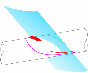
Considering the distinctive three-dimensional effects induced by the curved boundary layer in PISCBLIs, a qualitative analysis was conducted to elucidate the shock structure derived from the spatial flow field, depicted in figure 11. The reversed flow region, highlighted in pink, exhibits a short and broad curved profile, with its spanwise width slightly increasing in the downstream direction. Notably, the reversed flow region initially curves downward and subsequently upward in the vertical direction, forming a miniature bump along the streamwise direction. A prominent feature is the presence of a minor depression distributed along the spanwise direction within the separation bubble, where a portion of the airflow deflects laterally on both sides. In the central region ($0 \le z/D < 0.3$), the angle and streamwise position of the incident shock remain almost invariant. As a result, the ‘shock triangle’ structure and the separation region exhibit consistent shapes along the spanwise direction. However, owing to the swept-back nature of the separation bubble, the position of the compression shock shifts downstream along the spanwise direction, resulting in a backward motion of the shock intersection point. Additionally, the height of shock intersection points diminishes along the spanwise direction due to the downward bending of the wall, leading to a reduction in the size of the ‘shock triangle’ structure. However, in the outer region ($z/D > 0.3$), the ramp shock sweeps backward along the spanwise direction, substituting the incident shock interaction with a swept shock interaction. The curved swept-back shock interacts with the curved boundary layer, leading to the formation of a Mach stem structure, without reversed flow emerging in this region.

Figure 11. The distribution of the spanwise flow structure and separation near the cylinder wall.

The flow field structures represented in six spanwise slices, as depicted in figure 11, are extracted and illustrated in figure 12, where the $z/D = 0$ section represents the symmetry plane, with the other sections being parallel to it. Within a specific range of $0 < z/D < 0.3$, there is a descending scale of the ‘shock triangle’ structure in the flow field. Upon reaching the edge of the shock generator width at $z/D = 0.3$, the ‘shock triangle’ structure dissipates and is supplanted by a typical four-shock intersection configuration. For spanwise distances exceeding the shock generator width ($z/D > 0.3$), an inclined Mach stem appears in the flow field (figure 12e,f), which continuously increases in height with the increase in spanwise distance $z/D$. As illustrated in figure 13, the state of the airflow behind the intersection of the incident and separation shock on the symmetry plane ($z/D = 0$) is represented as $D_{30}$, necessitating a compression wave to counterbalance downstream pressure. As the spanwise distance increases, fluid within the central separation region diverts and accumulates laterally, resulting in a continuous increase in the height of the local separation bubble. Consequently, the separation shock intensifies, leading to a substantial increase in the airflow deflection angles. Behind the separation shock, the airflow parameter $D_2$ moves along the shock polar of $D_0$ in the direction of a growing deflection angle. The intersection point between the separated shock wave and the incident shock wave gradually shifts from $D_{30,a}$ to $D_{30,d}$, eventually leading to the complete disappearance of the refracted compression wave, corresponding to two polar curves that no longer intersect.

Figure 12. Flow field structure at different cross-sections along the spanwise direction: (a) $z/D = 0$; (b) $z/D = 0.1$; (c) $z/D = 0.2$; (d) $z/D = 0.3$; (e) $z/D = 0.4$; ( f) $z/D = 0.45$.

Figure 13. Schematic diagram of shock-polar at different spanwise positions; isentropic polar ($IP$)

The shock refraction phenomenon and the formation of the ‘shock triangle’ structure cease beyond two side plates. At this point, a Mach stem emerges between the incident shock and separation shock, which continuously increases in height along the spanwise direction. Moreover, the accumulation of low-energy fluids on both sides significantly results in a significant thickening of the boundary layer. However, there is no discernible reversed flow, and the airflow within the boundary layer no longer reverses but instead deflects towards the cylinder wall. Simultaneously, the separation shock dissipates and is replaced by a series of compression waves, which increases the Mach number behind them when compared with the region behind the separation. Furthermore, the airflow parameters located downstream of the compression wave can be simplified as points on the isentropic polar line in the shock-polar diagram. As shown in figure 13, the curve $n$ between points $D_{30,e/f}$ and $D_{40}$ represents the Mach stem, which inclines to a certain degree due to different pressure rises at varied deflection angles. As the angle of the compression wave increases, the deflection angle of the downstream airflow ascends, causing the shock polar emanating from point $D_2$ to shift to the upper right-hand side. Consequently, the height of the Mach stem accordingly increases as the point $D_{30}$ shifts to the right-hand side.

By analysing the flow fields on the inner and outer sides of the side plate, one can observe a clear transition from a ‘shock triangle’ structure to a Mach stem configuration, along with notable discrepancies in the shock refraction phenomenon within the boundary layer. The flow structure in the $(e)$ and $(f)$ sections is analysed through a simplified schematic representation and shock polar analysis. Figure 14 illustrates the schematic flow pattern beneath the Mach stem within the boundary layer. Upon entering the boundary layer, the transmitted shock $ts_1$ continuously bends, reflecting a series of expansion waves instead of compression waves (as shown in figure 12e,f). This behaviour contributes to the elimination of the ‘shock triangle’ structure following the shock intersection. Another significant observation is that the subsonic airflow is supremely superseded by fully supersonic airflow behind the transmitted shock $ts_1$, while the sonic line retains a shape congruent with that of the boundary layer.

Figure 14. Refraction of the shock in the shock coalesced region: $t_1$, $t_2$, $t_j$, $t_n$, the refraction of transmitted shock in the boundary layer; $D_{30}$, $D_{31}$, $D_{32}$, $D_{3j}$, $D_{3n}$, the airflow parameters behind shock $ts_1$, $t_1$, $t_2$, $t_j$, $t_n$; $sl_1$, $sl_2$, slip line; here boundary layer BL; sonic line SL. Here $0.3 < z/D < 0.5$, Mach reflection (MR).

The shock refraction principle between the Mach stem and the sonic line is elucidated in greater depth through the shock polar, as depicted in figure 15. The shock angle of the Mach stem, denoted as $n$, increases continuously, ultimately gradually transforming into a normal shock. At both ends of the Mach stem, two slip lines are pulled out, with the airflow states on either side of these slip line represented as the identical points ($D_{30}$–$D_{50}$, $D_{40}$–$D_{60}$) on the shock polar. Consequently, as one moves from $D_{40}$ to $D_{30}$, the deflection angle of the airflow behind the Mach stem diminishes progressively, while the pressure experiences a minor increase. The region situated behind the Mach stem (the state between $D_{30}$ and $D_{40}$) is entirely occupied by subsonic airflow, which transitions to supersonic at the lower end of the Mach stem. When the transmitted shock $ts_1$ penetrates the boundary layer, the reduction in incoming airflow velocity alters the angle of the transmitted shock, increasing from $t_1$ to $t_2$, $t_j$, until $t_n$, which results in a corresponding decrease in the deflection angle of the airflow. Furthermore, the decline in incoming Mach number, combined with the rise in the angle of the transmitted shock, leads to a reduction in the Mach number downstream until the sonic line established beneath the shock $t_n$. The airflow following the transmitted shock migrates downward to the right-hand side, approaching the sonic line $S_0$, dictated by the variation trend of airflow deflection angle and Mach number. From $D_{30}$ to $D_{31}$, and subsequently to $D_{3j}$, until $D_{3n}$, a series of expansion waves expand the airflow. In this intense three-dimensional flow, not only is there a modification in the near-wall separation flow, but also a fundamental transformation in the refractive phenomenon and diffraction characteristics adjacent to the boundary layer.

Figure 15. The expression of shock refraction in the shock-polar diagram: $0.3 < z/D < 0.5$.

3.4. Separation flow patterns near the cylinder wall

Considering that the most prominent characteristic of the boundary layer on the cylinder, which is a curved surface with constant curvature, it is crucial for investigating the flow pattern exhibiting a three-dimensional effect on the cylinder wall. Figure 16 displays experimental and numerical oil-flow images of PSWCBLIs, where points ‘$S$’ and ‘$N$’ denote the saddle point and node point; red and purple dashed lines mark primary and secondary separation lines. Starting from the node point, airflow within the separation bubble deflects to the mainstream direction, then detaches from the wall at the primary separation line, and eventually reattaches to the cylinder wall at the reattachment line after a certain distance. In contrast to typical ISWBLIs on flat plates, the primary separation line of PISCBLIs exhibits a curved swept-back shape, with its curvature continuously increasing along the spanwise direction. This separation line converges into an asymptote on the leeward side of the cylinder, aligned with the mainstream direction. Furthermore, the reattachment line emitted from the nodes also exhibits a swept-back shape, bending opposite to the separation line direction. The flow field between the primary separation line and the reattachment line is intricate, showcasing a significant three-dimensional effect. Moreover, the secondary separation is generated on both sides of the cylinder wall, constituting an open-type separation observed on the wall where the airflow converges to a secondary separation line without a distinct starting edge. As this secondary separation is located on the leeward side of the cylinder, its traces are captured in the oil-flow pattern from the vertical view. In the experimental images on the left-hand side, there is an accumulation phenomenon near the primary separation line, but no significant oscillation is observed in the oil-flow streak-line patterns across the entire separation region. Even though Squire (Reference Squire1961) noted that oil streaks may underestimate the distance to separation, the shock-induced separated regions shown in the oil-flow visualization here remain highly reliable.

Figure 16. Experimental and numerical oil-flow patterns taken from different directions: (a) side view; (b) vertical view. Here separation line $SL$; reattachment line $RL$; asymptote line $AL$; saddle point $S$; node point $N$.

The flow patterns on the cylinder wall, captured from vertical and side views, are integrated to enhance observation and facilitate further quantitative analysis. A coordinate transformation and normalization process, expressed in the arclength formulation and azimuthal angle, was to convert flow field parameters on the cylindrical surface into a rectangular coordinate system. Figure 17 illustrates the schematic diagram of the numerical wall streamline, where surface shear stress lines are transformed based on curve length and azimuthal angle, as follows:

(3.1)\begin{gather} \varphi=\arcsin\left({\frac{{z}}{{y}^{2}+{z}^{2}}}\right), \end{gather}

(3.2)\begin{gather} l=\varphi\sqrt{{y}^{2}+{z}^{2}}, \end{gather}

(3.3)\begin{gather} F_{r}=F_{y}\cos{\varphi}+F_{z}\sin{\varphi}, \end{gather}

(3.4)\begin{gather} F_\tau=F_{z}\cos{\varphi}-F_{y}\sin{\varphi}, \end{gather}

where $y$ and $z$ represent the coordinates in the vertical and spanwise directions, respectively, and $l$ is the arclength associated with $\varphi$. Here $F$ represents any physical vector in the three-dimensional flow field. The coordinates are converted from the $x$–$y$ coordinate system to the $r$–$\tau$ coordinate system by introducing different vector parameters into $F$. The normalized flow field after the coordinate transformation is depicted in figure 17, with main flow structures marked. Red and green dots represent saddle and node points on the centreline, respectively. Purple dotted lines, purple lines and red solid lines mark the upstream influence line, primary separation line ($SL_1$) and the secondary separation line ($SL_2$), respectively. Meanwhile, the interaction length ($\Delta x_{int}$) is defined as the distance along the streamwise between the upstream influence line (onset of the pressure rise, $x_{s,ts}$) and the saddle point ($x_{r,ts}$), while the separation length in the centreline ($\Delta x_{sep}$) is the distance from the saddle points in the centreline ($x_{s,ts}$) to the node point ($x_{r,ts}$). The circumferential widths from the downstream positions of the primary and secondary separation lines to the centreline are designated as $\Delta w_{s_1}$ and $\Delta w_{s_2}$, respectively. The transformed parameters pertinent to the separation regions are presented in table 2.

Figure 17. Schematic diagram of numerical surface streamline; cylindrical surface transformed into a rectangular plane.

Table 2. Transformed parameters of the flow patterns on the cylinder wall.

Figure 18 depicts the three-dimensional vortex structure in the near-wall region. Two counter-rotating vortices, identified using the $Q$-criterion, warp up around the cylinder and flow along the streamwise direction. The primary vortex experiences a significant deflection angle, approximately emanates from the initiation of the reversed flow region, where the airflow experiences a significant deflection angle, approximately $180^\circ$ before colliding with the mainstream in front of the primary separation line. This vortex constantly entraining the airflow between the primary separation line and the reattachment line, while expanding in its size with a swept-back shape along the spanwise direction. As the primary vortex moves to both sides, it gradually approaches the cylinder wall, and its scale and intensity continuously decrease. The secondary flow vortex tightly adheres to the secondary separation line on the wall (figure 16). Alvi & Settles (Reference Alvi and Settles1992) proposed that the normal Mach number $M_n = M_0\sin \beta _0$ is the critical parameter determining the swept shock–boundary layer interactions phenomenon, and when $1.5 < M_n < 1.9$, the lateral flow is pronounced, and secondary separation phenomenon emerges near the wall. However, in this study, the normal Mach number $M_n$ was slightly less than 1.5, yet secondary separation was still observed near the cylinder. This finding suggests that PISCBLIs on the curved boundary layer induce more substantial lateral flow than on the flat plate, and secondary separation emerges with a smaller normal Mach number $M_n$.

Figure 18. Vortex structure of different perspectives in the near-wall region based on $Q$ criterion given by CFD: 1, the primary vortex; 2, the secondary vortex.

The two separation vortices occupy the region above the primary separation line and the reattachment line and gradually dissipate along the asymptote in the downstream direction. The velocity of the fluids within the secondary vortex, as indicated in the velocity distribution legend, is markedly lower, reflecting a substantially reduced intensity compared with that of the primary vortex. The overall vortex structure generally exhibits the same swept shape as the separation line, curling along the side of the cylinder where the planar shock impinges. Previous research results (Stephen et al. Reference Stephen, Farnsworth, Porter, Decker, McLaughlin and Dudley2013) have characterized this vortex structure as a ‘concave horseshoe-shaped’ cluster. Furthermore, the primary vortex exhibits significantly more prominently in scale and height than the secondary vortex. As the two vortices gradually develop downstream, they become more constrained by the cylinder wall, resulting in an alteration of their shapes and eventually evolving into a quasielliptical configuration.

3.5. Patterns of time-mean pressure distribution on the cylinder wall

Figure 19 presents the time-averaged static pressure distribution on the cylindrical surface at various circumferential positions ($\varphi = 0^\circ$, $20^\circ$, $60^\circ$, $100^\circ$ and $180^\circ$), combining both experimental and CFD results. The red and green dotted lines in the figure represent the saddle and node points on the centreline ($\varphi = 0^\circ$), as determined in the oil-flow diagram. Notable characteristics of the separated flow within the central region of the windward side ($0^\circ < \varphi < 20^\circ$) are specifically manifested in a sharp initial increase in pressure at the interaction onset, followed by a pressure plateau. The reattachment process then occurs, exhibiting a more gradual ascent in pressure compared with the separation process. Following the attainment of the peak value at the node point, there is a progressive descending trend in pressure, attributed to the influence of the shoulder expansion fan. In the spanwise direction, the angle between the incident shock and the normal direction of the wall increases, resulting in a decreased adverse pressure gradient in the normal direction. The value of pressure plateau associated with the separation diminishes due to the intensification of lateral flow. In regions situated far from the centreline on the windward side ($60^\circ < \varphi < 180^\circ$), the peak pressure significantly decreases and the pressure plateau disappears. Furthermore, the initiation of the upstream pressure rise shifts backwards, indicating an upstream effect provoked by the swept-back pattern of the incident planar shock on the cylinder.

Figure 19. Comparison of time-average pressure distribution along the streamwise.

To elucidate the changes in the pressure plateau values mentioned previously, theoretical calculations are performed using the free interaction theory (FIT) (Chapman, Kuehn & Larson Reference Chapman, Kuehn and Larson1958), where the pressure rise during the free-interaction process is expressed as follows:

(3.5)\begin{equation} {p}/{p}_0=1+F\left({\bar{x}}\right)\frac{\gamma}{2}M_0^2\sqrt{\frac{2C_{f,0}}{\left({M_0^2-1}\right)^{0.5}}}, \gamma = 1.4, \left\{\begin{array}{@{}l@{}} {F(\bar{x})}_{s,point} = 4.2,\\ {F(\bar{x})}_{s,plateau} = 6.0, \end{array}\right. \end{equation}

where $F(\bar {x})$ is a universal correlation function, $F(\bar {x})_{spoint}$ and $F(\bar {x})_{splateau}$ represent the values at the separation point and the separation plateau under turbulent separation, respectively. Here $\gamma$ is the specific heat ratio. Based on the obtained boundary layer parameters of the incoming flow, the theoretical pressure rise of the separation point $(p_{t,spoint} / p_0 = 1.52)$ and separation plateau $(p_{t,splateau} / p_0 = 1.74)$ are obtained by substituting $C_{f,0}$ and $M_0$ into the relations (3.5). Moreover, the theoretical shock angle ($\alpha _s=40.22^\circ$) induced by separation under free interaction can be calculated by the pressure ratio relationship of the oblique shock.

The pressure ratio and separation shock angle are quantified across various spanwise sections utilizing pressure distribution measurements and schlieren imaging in both experimental and CFD analyses. The results are presented in table 3, where ‘Error’ denotes the relative difference between measured and theoretical values for these parameters. A comparative analysis reveals that, while the separation shock angle significantly increases along the spanwise direction, the pressure rise in the separation region (including the separation point and separation plateau) progressively decreases. This pressure change indicates that the increase in pressure rise caused by the separation shock cannot offset the decrease in pressure rise caused by lateral flow, which ultimately generates a spanwise pressure gradient. Consequently, these results lead to the release of high pressure in the separation region along with low-energy fluids. Near the symmetry plane, the interaction adheres to the FIT, as evidenced by the consistent separation shock angles and pressure increases observed on the cylindrical surface. However, as the spanwise distance increases, the measured values of separation shock angle and pressure rise show a continuously increasing difference compared with the theoretical values, signifying a gradual departure from FIT at positions on either side of the cylinder.

Table 3. The measured values and relative error of the different spanwise sections; the section $z/D = 0$ represents the symmetry plane.

An analysis of the oil-flow patterns on the cylindrical surface indicates that PISCBLIs do not adhere to conical or cylindrical similarity in swept shock–boundary layer interaction. When the cylindrical surface is transformed into a rectangular plane, an elliptical configuration of the separation line of the cylindrical surface inside two side plates is unveiled. This elliptical formation bears resemblance to the intersection line of the planar incident shock on the cylinder wall. In figure 20, elliptic polar coordinates are introduced into the transformed cylindrical plane. The position of the elliptical coordinate system is established based on the separation line, where $\theta$ denotes the inclined angle between the polar axis and the $x$-axis, $\rho$ symbolizes the distance between any point on the polar axis and the origin and $\rho _0$ represents the distance between the point on the central separation line and the origin. The centre of the ellipse is located precisely at the extremum of the pressure, from which to the upstream influence line, the pressure distribution on the cylinder wall exhibits a radial shape. Pressure on different angular polar axes is extracted from experimental and CFD results, and the dimensionless pressure distribution curve is drawn with $\rho _0$ as the benchmark, as shown in figure 21. Notably, it is observed that the pressure curves at different angles coincide, demonstrating a consistent pressure distribution in line with the elliptical similarity property.

Figure 20. Schematic diagram of the establishment of the elliptic coordinate system.

Figure 21. Pressure distribution curve on the polar axis at different angles in the elliptical coordinate system.

This elliptical similarity fundamentally correlates with the approximate elliptical intersection line formed by the incident shock impinging on the cylindrical surface. Evidently, this elliptical similarity feature does not encompass the entirety of the separation region but is only limited to most of the reversed flow region. The primary reason for this phenomenon lies in the constrained width of the incident shock, which is limited to the region between the two side plates, allowing the incident shock to maintain a planar configuration and a constant intensity. However, the incident shock sweeps back outside the side plates, resulting in a notable enhancement of the three-dimensional effects. Consequently, its strength is diminished considerably in the spanwise direction, making a huge difference in adverse pressure gradient. In the region of a large polar angle ($\theta > 50^\circ$ or $z/D > 0.3$), the pressure distribution gradually deviates from this law. Notably, at the centre of the separation region, the lateral pressure gradient forces low-energy fluids to accumulate on both sides, resulting in a rapid decrease in pressure plateau values outside the side plates, far from the centre. This correlates with the phenomenon of pressure similarity deviating as the polar angle increases in figure 21. Therefore, the elliptical similarity criterion is only valid within the confines of the region between the side plates.

3.6. Potential unsteady behaviour

The time-averaged flow field characteristics of PISCBLIs are elucidated through the aforementioned schlieren images, pressure distribution and surface oil-flow topology. Notably, the separation flow induced by PISCBLIs exhibits certain unsteady behaviours, which are subsequently evaluated through various transient measurement techniques to ascertain whether these behaviours can trigger substantial alterations in the flow structure (Clemens & Narayanaswamy Reference Clemens and Narayanaswamy2014). The low-frequency oscillation observed in the separation region is often accompanied by fluctuations in the surface pressure, therefore the dynamic pressure measurement method is utilized to capture and analyse the unsteady oscillation features within the separation region. In order to effectively capture low-frequency oscillation signals of the separation region, the measurement points of dynamic pressure are strategically positioned slightly upstream and downstream of the separation point along the centreline, with their positions indicated in figure 6.

Figure 22 presents the transient surface pressure, which clearly demonstrates a regular pattern of low-frequency oscillation. The amplitude of the pressure fluctuation signal $p^,/p_d$ $(-0.014, 0.017)$ corresponds to the oscillation range of the separation shock $\beta ^,/\beta _2$ $(-0.0086, 0.0097)$, where the $p_d$ and $\beta _2$ represent the pressure at local measuring points and angle of separation shock, respectively. Further spectral analysis was conducted to address unsteady aspects related to separation dynamics, where the Welch method was used to calculate the power spectral density (PSD) of the pulsating pressure. As shown in figure 23, the energy of the pressure signal of both upstream boundary layer and separation bubble is mainly concentrated in the range of the low frequency, and the PSD gradually decreases with frequency. In order to better reflect the energy spectrum features of pressure fluctuation in the range of low frequency, the weighted PSD (WPSD) was obtained by the weighting of frequency. The WPSD curve of the pressure signal at the separation point reveals a pronounced peak in the low-frequency spectrum, with the characteristic frequency corresponding to the peak point determined to be 205 Hz, yielding a Strouhal number $St_L$ of 0.0094. This Strouhal number is non-dimensionalized based on the streamwise length of the separation bubble on the centreline and the velocity of incoming flow. Clemens & Narayanaswamy (Reference Clemens and Narayanaswamy2014) discovered that in the two-dimensional SBLIs, the dimensionless characteristic frequency $St_L$ of low-frequency oscillation is between 0.01 and 0.03. In the case of the PISCBLIs examined in this study, the Strouhal number of the low-frequency oscillation is relatively small, mainly due to the unique three-dimensional lateral flow that reduces the streamwise length of the separation region.

Figure 22. Pressure fluctuation signal on the wall surface.

Figure 23. Fluctuating pressure signal of the upstream boundary layer and separation point: (a) PSD; (b) associated weighted PSD function.

As shown in figure 12, figure 12(a–c) represent the state of the flow field in the central region, and figure 12(e–f) represent the state of the flow field in the two sides. Figure 12(d), positioned adjacent to the side plate, depicts a transitional flow field state bridging the central region and the lateral sides. In order to elucidate the effects of the impact of aforementioned low-frequency oscillation on macroscopic flow field structures and three-dimensional flow characteristics, the inviscid ${\rm RR} \leftrightarrow {\rm MR}$ transition criteria in the ($\delta _1$, $\delta _2$) plane for $Ma_0 = 2$ and $\gamma = 1.4$ is shown in figure 24. Although the separation shock angle and airflow deflection angle ($\delta _2$) has increased in the central region (from figure 12a to figure 12c), the flow structure remains within the RR region. Conversely, as the separation shock angle continues to rise from the central area to both lateral sides (from figure 12c to figure 12f), the flow field structure enters the RR region, with the transition location occurring outside of the side plate. The analysis reveals that the fluctuations caused by the PISCBLIs itself or the low-frequency oscillations are insufficient to initiate the transition from RR to MR for the considered flow conditions. As low-energy fluid accumulates towards both sides due to the lateral flow effect, an increase in the angle of the compression wave induced the flow to completely transform into MR. Similarly, the low-frequency oscillations here are insufficient strong to return to the RR. Hence, the ${\rm RR} \leftrightarrow {\rm MR}$ transition predominantly driven by the increase in the angle of separation shock (or compression wave), rather than through unsteady disturbance. In figure 12(d), characterized as transitional and situated near the side plate, the flow exhibits considerable complexity, displaying unsteady behaviours that engender mutual transformations between RR and MR. Note that these interactions occur primarily on a microscopic scale.

Figure 24. Analytical results for the ${\rm RR} \leftrightarrow {\rm MR}$ transition criteria in the ($\delta _1$, $\delta _2$) plane for $Ma_0 = 2$ and $\gamma = 1.4$: (a) $z/D = 0$; (b) $z/D = 0.1$; (c) $z/D = 0.2$; (d) $z/D = 0.3$; (e) $z/D = 0.4$; ( f) $z/D = 0.45$. Sonic ($\delta ^S$) criteria as proposed by Hu et al. (Reference Hu, Myong, Kimand and Cho2009); detachment ($\delta ^D$) as proposed by Li, Chpoun & Ben-dor (Reference Li, Chpoun and Ben-dor1999) for asymmetric shock intersections.