2.1. Governing equations and numerical method

The numerical simulation of aerobreakup is a computationally demanding task due to the broad physics occurring at a large range of spatio-temporal scales. In general, aerobreakup is governed by the compressible Navier–Stokes for the liquid and surround gas flow, and coupled by continuity and an equality of stresses at the deforming surface. This can be modelled by coupling two solvers or, more commonly, by adopting a volume-of-fluid approach and either explicitly tracking the interface or by capturing a slightly diffused interface on the grid (Fuster Reference Fuster2019; Saurel & Pantano Reference Saurel and Pantano2018). Examples of interface-tracking approaches include free-Lagrange methods (Ball et al. Reference Ball, Howell, Leighton and Schofield2000), level-set/ghost-fluid approaches (Abgrall & Karni Reference Abgrall and Karni2001; Liu, Khoo & Yeo Reference Liu, Khoo and Yeo2003; Liu, Yuan & Shu Reference Liu, Yuan and Shu2011; Pan et al. Reference Pan, Han, Hu and Adams2018) or front-tracking schemes (Cocchi & Saurel Reference Cocchi and Saurel1997). While such interface-tracking approaches have the advantage of a well-defined, sharp interface between components and thus (potentially) accurate interface dynamics, various issues ranging from spurious pressure oscillations near the interface to lack of conservation make these schemes less suitable for shock-dominated flows or aerobreakup (see, e.g. Fuster (Reference Fuster2019) and Saurel & Pantano (Reference Saurel and Pantano2018) for recent reviews on the topic).

Hence, to accurately simulate aerobreakup of a water droplet, we resort to an interface-capturing scheme, combining a multicomponent flow model with a shock-capturing finite-volume method. These schemes are also known as diffuse interface methods as the interface is not sharp and tracked explicitly but the scheme permits some numerical diffusion of the interface. This allows for discrete conservation, consistent thermodynamics in mixture cells and dynamically appearing or vanishing interfaces. In addition, diffuse interface methods are generally more efficient compared to their interface-tracking counterpart, which is crucial for multi-scale problems such as aerobreakup.

While there exist a variety of multicomponent models, we consider immiscible fluids in mechanical equilibrium and use the model of Kapila et al. (Reference Kapila, Menikoff, Bdzil, Son and Stewart2001). However, to ensure robustness and stability of the scheme, a pressure-relaxation method is used to converge from a pressure-disequilibrium formulation to mechanical equilibrium (Saurel, Petitpas & Berry Reference Saurel, Petitpas and Berry2009). While valuable insight has been obtained with numerical studies of aerobreakup in the past (see, e.g. Jalaal & Mehravaran Reference Jalaal and Mehravaran2014; Garrick Reference Garrick2016; Liu et al. Reference Liu, Wang, Sun, Wang and Wang2018; Meng & Colonius Reference Meng and Colonius2018; Liu et al. Reference Liu, Wang, Sun, Deiterding and Wang2019; Marcotte & Zaleski Reference Marcotte and Zaleski2019), the computational costs quickly become prohibitive for the large range of scales in aerobreakup. Hence, most commonly, artificial symmetries are imposed, which prohibit the formation of truly three-dimensional instabilities or do not account for any viscous or capillary effects, which become important at later stages of the breakup. In order to capture these effects, we model surface tension as proposed in Schmidmayer et al. (Reference Schmidmayer, Petitpas, Daniel, Favrie and Gavrilyuk2017) and viscous effects are accounted for by extending the models for mechanical equilibrium (Thévand, Daniel & Loraud Reference Thévand, Daniel and Loraud1999; Périgaud & Saurel Reference Périgaud and Saurel2005; Coralic & Colonius Reference Coralic and Colonius2014) to the non-equilibrium-pressure model. For a notable study on the relevance of both viscous and inviscid instability mechanisms in the context of two-phase mixing layer, we refer to Matas (Reference Matas2015).

The viscous, non-equilibrium-pressure multicomponent model with surface-tension effects for two components reads as

(2.1)\begin{equation} \left. \begin{array}{c} {\dfrac{{\partial {\alpha _1}}}{{\partial t}} + \boldsymbol{u} \boldsymbol{\cdot} \boldsymbol{\nabla} {\alpha _1}} = {\mu ( {{p_1} - {p_2}} ) ,} \\ {\dfrac{{\partial {\alpha _1}{\rho _1}}}{{\partial t}} + \boldsymbol{\nabla} \boldsymbol{\cdot} ( {{\alpha _1}{\rho _1}\boldsymbol{u}} )} ={0 ,} \\ {\dfrac{{\partial {\alpha _2}{\rho _2}}}{{\partial t}} + \boldsymbol{\nabla} \boldsymbol{\cdot} ( {{\alpha _2}{\rho _2}\boldsymbol{u}} )} ={ 0 ,} \\ {\dfrac{{\partial \rho \boldsymbol{u}}}{{\partial t}} + \boldsymbol{\nabla} \boldsymbol{\cdot} ( {\rho \boldsymbol{u} \otimes \boldsymbol{u} + p \boldsymbol{\mathsf{I}} + \boldsymbol{\varOmega} -{\boldsymbol \tau} } )} = { \boldsymbol 0 ,} \\ {\dfrac{{\partial {\alpha _1}{\rho _1}{e_1}}}{{\partial t}} + \boldsymbol{\nabla} \boldsymbol{\cdot} ( {{\alpha _1}{\rho _1}{e_1}\boldsymbol{u}} ) + {\alpha _1}{p_1}\boldsymbol{\nabla} \boldsymbol{\cdot} \boldsymbol{u}} = { - \mu {p_I} ( {{p_1} - {p_2}} )+\alpha_1 {\boldsymbol \tau}_1\boldsymbol{:} \boldsymbol{\nabla} \boldsymbol{u} ,} \\ {\dfrac{{\partial {\alpha _2}{\rho _2}{e_2}}}{{\partial t}} + \boldsymbol{\nabla} \boldsymbol{\cdot} ( {{\alpha _2}{\rho _2}{e_2}\boldsymbol{u}} ) + {\alpha _2}{p_2}\boldsymbol{\nabla} \boldsymbol{\cdot} \boldsymbol{u}} = { \mu {p_I} ( {{p_1} - {p_2}} ) +\alpha_2 {\boldsymbol \tau}_2\boldsymbol{:} \boldsymbol{\nabla} \boldsymbol{u} ,} \\ {\dfrac{{\partial c}}{{\partial t}} + \boldsymbol{u} \boldsymbol{\cdot} \boldsymbol{\nabla} c} = { 0 ,} \end{array} \right\} \end{equation}

where $\alpha _k$, $\rho _k$, $e_k$ and $p_k$ indicate the volume fraction, the density, the internal energy and the pressure of component $k$. Identity is denoted by $\boldsymbol{\mathsf{I}}$. The mixture variables for density, pressure and velocity are denoted by $\rho$, $p$ and $\boldsymbol {u}$, respectively and are given by

(2.2a,b)\begin{equation} \rho = \sum_{k=1}^2 \alpha _k \rho_k \quad \text{and} \quad p = \sum_{k=1}^2 \alpha _k p_k. \end{equation}

The capillary tensor reads

(2.3)\begin{equation} {\boldsymbol \varOmega} = - \sigma \left( {\| {\boldsymbol{\nabla} c} \| \boldsymbol{\mathsf{I}} - \frac{{\boldsymbol{\nabla} c \otimes \boldsymbol{\nabla} c}}{{\| {\boldsymbol{\nabla} c} \|}}} \right), \end{equation}

where $\sigma$ is the surface-tension coefficient and $c$ is a colour function. The viscous stress tensor for the mixture is given by

(2.4)\begin{equation} {\boldsymbol \tau}=2\eta ( \tfrac{1}{2}( \boldsymbol{\nabla} \boldsymbol{u} + (\boldsymbol{\nabla} \boldsymbol{u})^T)- \tfrac{1}{3}(\boldsymbol{\nabla} \boldsymbol{\cdot} \boldsymbol{u}) \boldsymbol{\mathsf{I}} ), \end{equation}

where $\eta$ is the mixture shear viscosity and the viscous stress tensor for component $k$ is denoted by ${\boldsymbol \tau }_k$. The pressure-relaxation coefficient is given by $\mu$ and the interfacial pressure is

(2.5)\begin{equation} {p_I} = \frac{{{z_2}{p_1} + {z_1}{p_2}}}{{{z_1} + {z_2}}}, \end{equation}

where ${z_k} = {\rho _k}{a_k}$ is the acoustic impedance of component $k$. Note that the pressure-relaxation terms can be obtained from the asymptotic limit of the Baer & Nunziato (Reference Baer and Nunziato1986) model in the limit of stiff velocity relaxation (see also Saurel et al. (Reference Saurel, Petitpas and Berry2009) for further details).

Due to $p_1 \neq p_2$ in this model, the total-energy equation of the mixture is replaced by the internal-energy equation for each component. Nevertheless, the mixture-total-energy equation of the system can be written in the usual form

(2.6)\begin{equation} \frac{{\partial \rho E + \varepsilon _\sigma}}{{\partial t}} + \boldsymbol{\nabla} \boldsymbol{\cdot} ( {( {\rho E + \varepsilon _\sigma + p} ) \boldsymbol{u} + \boldsymbol{\varOmega} \boldsymbol{\cdot} \boldsymbol{u} - {\boldsymbol \tau} \boldsymbol{\cdot} \boldsymbol{u}} ) = 0 , \end{equation}

where the total energy is

(2.7)\begin{equation} E = e + \tfrac{1}{2} \| \boldsymbol{u} \|^2, \end{equation}

and the internal energy is given by

(2.8)\begin{equation} e = \sum_{k=1}^2 Y_k e_k ( \rho_k , p_k ). \end{equation}

The capillary energy reads

(2.9)\begin{equation} {\varepsilon _\sigma } = \sigma \| {\boldsymbol{\nabla} c} \|. \end{equation}

Note that (2.6) is redundant when solving internal-energy equations for both components. However, it is included to ensure total-energy conservation also numerically (see Saurel et al. (Reference Saurel, Petitpas and Berry2009) for further details).

In (2.8), $e_k$ is defined via an equation of state and $Y_k$ are the mass fractions

(2.10)\begin{equation} Y_k = \frac{\alpha_k \rho_k}{\rho}. \end{equation}

Here, we consider a two-phase mixture of gas ($g$) and liquid ($l$). The gas is modelled by the ideal-gas equation of state

(2.11)\begin{equation} p_g = ( \gamma_g - 1) \rho_g e_g , \end{equation}

with $\gamma _g = 1.4$. The liquid on the other hand is modelled by the stiffened-gas equation of state

(2.12)\begin{equation} p_l = ( \gamma_l - 1) \rho_l e_l - \gamma_l {\rm \pi}_\infty, \end{equation}

where $\gamma _l = 6.12$ and ${\rm \pi} _\infty = {3.43 \times 10^8}\ \textrm {Pa}$ (Coralic & Colonius Reference Coralic and Colonius2014; Meng & Colonius Reference Meng and Colonius2014, Reference Meng and Colonius2018).

Numerically, this model is solved in three steps, which are outlined below. First, the hyperbolic non-equilibrium-pressure model is solved by neglecting surface-tension and viscous effects and relaxation terms. Second, the viscous, surface-tension model is solved and, finally, in the last step, the pressure is relaxed until an equilibrium is reached. In summary, the model is solved with the following steps:

1. (i) Solve hyperbolic pressure-disequilibrium model using a Godunov-type method. At the volume–volume interfaces, the associated Riemann problem is computed using the HLLC (Harten–Lax–van Leer–Contact) approximate solver.

2. (ii) Solve the viscous, surface-tension model.

3. (iii) Infinite pressure relaxation ($\mu \to +\infty$), converging to the thermodynamically consistent, mechanical-equilibrium model, coupled with a re-initialization procedure ensuring conservation.

A second-order-accurate MUSCL (monotonic upstream-centred scheme for conservation laws) scheme with two-step time integration is used, where the first step is a predictor step for the second and the usual piecewise linear MUSCL reconstruction (Toro Reference Toro1997) is used for the primitive variables. In addition, the monotonized central (Van Leer Reference Van Leer1977) slope limiter is combined with the THINC (tangent of hyperbola for interface capturing) interface-sharpening technique to minimize interface diffusion (Shyue & Xiao Reference Shyue and Xiao2014).

In order to resolve the wide range of spatial and temporal scales of shock fronts and interfaces, an adaptive mesh refinement technique is employed (Schmidmayer, Petitpas & Daniel Reference Schmidmayer, Petitpas and Daniel2019). The refinement criteria are based on variations of volume fraction, density, pressure and velocity.

This methodology is implemented in the open-source code ECOGEN (Schmidmayer et al. Reference Schmidmayer, Petitpas, Le Martelot and Daniel2020b), which has been validated, verified and tested in various set-ups ranging from gas bubble dynamics problems, including free-space and wall-attached bubble collapses, liquid–gas shock tubes, surface-tension problems and water-column breakup due to high-speed flow (see, e.g. Schmidmayer et al. Reference Schmidmayer, Petitpas, Daniel, Favrie and Gavrilyuk2017, Reference Schmidmayer, Petitpas and Daniel2019; Pishchalnikov et al. Reference Pishchalnikov, Behnke-Parks, Schmidmayer, Maeda, Colonius, Kenny and Laser2019; Schmidmayer, Bryngelson & Colonius Reference Schmidmayer, Bryngelson and Colonius2020a).

2.2. Problem definition

Aerobreakup occurs when a liquid drop is suddenly exposed to a high-speed gas flow. These initial conditions are typically generated using a planar shock due to its simplicity, robustness and repeatability in both experiments and simulations without significantly interfering with the droplet or the evolution of the subsequent stages of the aerobreakup. In the simulation, we match the experimentally measured mean shock strength $M_s \sim 1.3$, the Reynolds number $Re = {u_s D_0}/{\nu }$ and the Weber number $We ={\rho _g u_s^2 D_0}/{\sigma }$, where $D_0$, $u_s$, $\nu$ and $\sigma$ denote the initial droplet diameter, the post-shock gas velocity, the kinematic viscosity of the gas and the surface-tension coefficient. In the experiments we mainly focus on the piercing regime with mean Weber numbers in the range of $We =[200, 700]$. Numerically, we conduct two simulations, where one matches a mean experimental Weber number of $We \sim 470$ and one does not have any surface-tension effects, which is denoted in the following as $We \to \infty$. Note that $We \to \infty$ is purely nomenclature and does not indicate the limiting process to infinite Weber number. In both cases the Reynolds number is set to $Re \sim 7000$. Hence, we numerically probe and compare both the piercing and the stripping regimes.

The simulations are carried out in rectangular computational domain, which is given by $[-7D_0, 15D_0] \times [-6D_0,6D_0]\times [-6D_0,6D_0]$. The domain size was chosen based on sensitivity studies, which aim to both minimize the influence of the domain boundary conditions and the computational effort. Our results are in line with previous studies (Meng & Colonius Reference Meng and Colonius2018). To capture the non-axisymmetric, three-dimensional modulation of the droplet and its surrounding flow field, we refrain from imposing any symmetries or simplifications and carry out full three-dimensional simulations for which the initial computational mesh and the set-up are shown in figure 1. The droplet is initially at rest and placed at the origin. On all domain boundaries, non-reflective boundary conditions (NRBC) are imposed. To ensure high spatial and temporal accuracy at reasonable computational costs, the adaptive mesh is composed out of four grid levels, which are adapted to follow the shocks, the interface and the turbulence. Here, we follow the methodology established and validated in Schmidmayer et al. (Reference Schmidmayer, Petitpas and Daniel2019), and refine cell $i$ for which the following criterion is fulfilled:

(2.13)\begin{equation} \frac{|X_{{Nb}(i,j)} - X_i|}{min (X_{{Nb}(i,j) } - X_i)} > \varepsilon, \end{equation}

where $X$ indicates a given flow variable and the criterion is tested for all neighbouring cells, indicated by the subscript $Nb(i,j)$, where the $j$th cell is the corresponding neighbour of cell $i$. The threshold is conservatively set to $\varepsilon =0.04$. For this set-up, we test the above refinement criterion for the flow variables density, velocity, pressure and volume fraction and refine the cell if the criterion is fulfilled for any of these variables. As a result, the initial droplet is resolved by $D_p=140$ points per diameter, which was increased compared to Meng & Colonius (Reference Meng and Colonius2018) in order to capture capillary effects such as the formation of ligaments during the course of the breakup. Note, however, that the selected resolution is by no means able to capture all fine-scale effects and the resolution required to do so would far exceed currently available computational resources, even on the largest of supercomputers (see, e.g. Meng & Colonius (Reference Meng and Colonius2018) for estimates). However, as shown in § 4, the good agreement of the simulation with our experiments suggest that the resolution is indeed sufficient to capture most pertinent effects of aerobreakup and all phenomena discussed here are observed both numerically and experimentally. The mesh adaptivity, following both the droplet interface and the shock is exemplified by a snapshot in figure 2 during the initial phase of the simulation. In addition, a conservative grid stretching towards the domain boundaries, as shown in figure 1, is used to further aid efficiency of the computations. Finally, to avoid spurious symmetries originating from the artificially symmetric initial conditions, we impose an initial velocity field with random perturbations of maximum ${O}(10^{-4} u_s)$. For the adaptive time marching scheme we maintain a maximum Courant–Friedrichs–Lewy number of $0.3$.

Figure 1. Initial computational mesh and set-up for the numerical simulation of aerobreakup.

Figure 2. Snapshot of the adaptively refined mesh, coloured by mixture pressure.

4.1. Droplet morphology

In order to compare the numerical simulation with images obtained from shadowgraphy in the following sections, we extract isosurfaces of volume fraction $\alpha _l=0.01$ from the simulation, and colour them by velocity magnitude (see, also figures 5 and 7). Note that diffuse interface methods, as employed here, can only provide a range in which the interface is likely to be found and by construction cannot provide an exact or deterministic location of the interface. While this leads to an ambiguous representation of the droplet surface, a sensitivity study in Meng & Colonius (Reference Meng and Colonius2018) led to the conclusion that isosurfaces of a volume fraction $\alpha _l=0.01$ are believed to be fair for comparison with experiments, considering the obscuring mist of the experiment, generated during the course of the breakup. Although this might seem a rather low volume fraction, it should be pointed out that this still corresponds to a mass fraction of $Y_l\approx 0.9$. For comparison of the numerical results with the experiment, we use, unless stated otherwise, the following non-dimensionalization

(4.1a,b)\begin{equation} {\boldsymbol x}^\ast=\frac{{\boldsymbol x}}{D_0}, \quad \tau= t\frac{{\boldsymbol u}_s}{D_0} \sqrt{\frac{\rho_s}{\rho}}, \end{equation}

where ${\boldsymbol x}$ and $t$ denote the dimensional location and time, respectively.

Figure 5. Numerical simulation of a water droplet aerobreakup (top two rows) and experimental visualizations (bottom rows). Characteristic times are (a) 0.00, (b) 0.27, (c) 0.47, (d) 0.72 and (e) 1.16. The timing information is for both experimental and numerical results expected for the numerical image (e) which corresponds to $\tau =1.01$. For the simulations, an isosurface of volume fraction $\alpha _l=0.01$ coloured by velocity magnitude is depicted from two different perspectives. The scale bar refers to experimental results. The Weber numbers in the simulation and the experiment are 470 and 492, respectively.

4.1.1. Finite Weber number case

At the first stages of the aerobreakup process ($\tau = 0.27 - 0.91$), the numerical results show the typical droplet shapes that experimental visualizations (figure 5) and the literature report, with a good qualitative agreement with our experiment. First, the initial droplet deforms into a muffin-like shape, described by a spherical upstream side with lips growing in the spanwise direction. The droplet core takes the shape of a conic cylinder and the downstream side is flattened into a planar interface ($\tau = 0.27$). While the droplet is continuously flattened, the stretching of lips in the streamwise direction results in a toroidal liquid rim ($\tau = 0.47$). Simultaneously, rear lips raise in the downstream side. Owing to inertial forces, the rim at the droplet periphery is stretched, which deforms the droplet into a crescent-like shape ($\tau = 0.72$). The rim begins to disintegrate into ligaments and subsequently into fragments. For characteristic times from 0.00 to 0.72, contours, extracted from the isosurfaces of the volume fraction $\alpha _l=0.01$ of the droplet, are overlaid on the experimental visualizations in figure 6. The contours are initially in good agreement with the experimental images. At later stages ($\tau = 0.72 - 1.16$), the numerical results and the experimental visualizations both show a periodic distribution of ligaments, although there are discrepancies in the precise shape. However, the ligament distribution in the numerical simulation is consistent with the distribution experimentally observed, as detailed below in § 5. Figure 5 shows that the toroidal rim is continuously sheared away with the flow for times $\tau = 0.72 - 1.16$, which leads to a cylindrical curtain surrounding the droplet core and a cavity behind. This results in a backward facing bag. The downstream end of the bag bends in the spanwise direction, forming a second rim, hindering the flow. Subsequently, the rim is subject to the development of multiple bags in the streamwise direction. Finally, bags are pierced by the flow, similar to the bag and multimode breakup regimes. The ligaments resulting from this piercing process are tied up to their ends by the annular ring. The periodic nature of the ligament distribution is further discussed in § 5.1. The droplet core develops a square-like shape (see, e.g. figure 5e). We believe this is a physical instability that results from preferred amplification of certain (even) azimuthal wavenumbers. While amplification of these same wavenumbers is also evident in the $We \to \infty$ simulation, the droplet in that case does not evolve into a coherent square shape. Therefore, as surface tension plays a role in the instability process, we speculate that it could be related to the polygonal instability (Labousse & Bush Reference Labousse and Bush2015) observed in other vortical-interfacial flows, but a definitive analysis awaits future work. In any simulation, available physical instabilities have to be seeded by disturbances that break the relevant symmetries, whether they are intentional (added to the initial conditions) or unintentional (seeded by discretization artifacts). As was observed previously by Meng (Reference Meng2016), an underlying Cartesian mesh appears to be capable, in the presence of a diffuse interface, to provide sufficient perturbation to axisymmetry to excite instabilities in a grid-aligned fashion, even though the instability itself is physical. In that study, cylindrical coordinates were preferred to eliminate this effect, especially because those simulations lacked physical viscosity to otherwise regularize the singularities associated with inviscid, interfacial flow (e.g. Kelvin–Helmholtz). With the present limits on resolution, we are therefore unable to offer a definitive conclusion on whether the ultimate square shape is independent of the numerics. While the present results qualitatively compare well with experimental images when viewing the droplet from the side, we are unable to view the droplet from upstream as would be required to directly view the square shape and directly validate the result.

Figure 6. Overlaying of droplet contours from numerical results (red lines) on experimental images at the early stages of the aerobreakup. Characteristic times are (a) 0.00, (b) 0.27, (c) 0.47 and (d) 0.72. The Weber number in the simulation and the experiment are 470 and 492, respectively.

4.1.2. Simulation without surface tension

Next, in order to isolate the effect of surface tension during the breakup, we conduct an additional numerical simulation and set the surface tension to zero with $M_{s}=1.3$ and $D_{0}=0.804$ mm and compare the results with experiments at a high Weber number of $We =1100$ ($M_{s}=1.3$, $d_{0}=1.68$ mm).

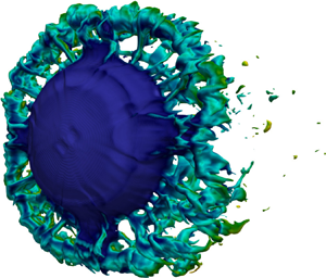
Figure 7 shows that the droplet morphology and the mechanisms observed bear resemblance to the finite Weber number case, especially in the early stages. The droplet is first deformed into a muffin-like shape with lips growing in the spanwise direction. Lips are rapidly sheared away with the flow by forming a liquid rim surrounding the droplet body. The rim stretches in the streamwise direction and forms a cylindrical curtain, which eventually results in a backward facing bag. Finally, and in contrast to the morphology previously observed in figure 5, much less distinct ligaments are formed and the liquid curtain breaks up directly into fine-scale structures due to a lack of the restoring surface-tension forces.

Figure 7. Numerical simulation of a water droplet aerobreakup and experimental visualizations. Characteristic times are (a) 0.00, (b) 0.20, (c) 0.52, (d) 0.73, (e) 0.86 and (f) 0.96. The scale bar refers to experimental results. In the experiment, the Weber number is $We =1100$, whereas the simulation does not account for surface-tension effects, i.e. $We \to \infty$.

4.2. Centre-of-mass evolution

Further validation is provided in figure 8 where the droplet centre-of-mass drift from the numerical simulation is compared with that measured in the experiments. From the numerical simulation the centre-of-mass is computed as in Meng & Colonius (Reference Meng and Colonius2018) using

(4.2)\begin{equation} {\boldsymbol x}_c= \frac{\displaystyle \int_{\varOmega_D} \alpha_l \rho_l {\boldsymbol x}{\textrm{d}V}}{\displaystyle \int_{\varOmega_D} \alpha_l \rho_l {\textrm{d}V}}, \end{equation}

where $\varOmega _D$ is the entire computational domain. On the experimental side, the evolution of the centre-of-mass is computed from 2-D planar images, due to the line-integrated nature of the images recorded by the shadowgraph. The centre-of-mass is determined by calculating the first-order spatial moment which is the intensity-weighted average of the pixel coordinates constituting the droplet. This requires a binary image. The binarization is performed by setting an intensity threshold to the image separating the droplet from the background. Despite a slight deviation due to the 2-D planar assumption and the threshold sensitivity, figure 8 shows a good quantitative agreement between numerical results and the experiments. It can be noticed that the surface tension has no discernible effect on the drift in the simulations. This observation is consistent with the similar droplet morphology observed in both simulations at $We = 470$ and $We \rightarrow \infty$.

Figure 8. Evolution of the centre-of-mass from numerical results and experimental observations. Error bars display the sensitivity of the centre-of-mass detection to the intensity threshold used in the binarization process.

5.1. Ligament formation and azimuthal modulation

Exposing the water droplet to a high-speed gas flow can induce a large difference in the velocities between the two fluids and thus destabilize their interface. Depending on the flow conditions, the interface may be more susceptible to Rayleigh–Taylor or Kelvin–Helmholtz instabilities. The canonical RTI occurs when a heavy fluid is suspended above a lighter fluid and both are subjected to acceleration. The interface begins to oscillate with alternating acceleration directions and is unstable when the acceleration is oriented towards the heavier fluid (Rayleigh Reference Rayleigh1882). On the other hand, KHI arises due to either shear in a single fluid system or due to a velocity difference across the interface of two fluids, which results in propagating waves that typically rollup into vortices along the interface (Chandrasekhar Reference Chandrasekhar1961).

For low Weber numbers ($We \sim 20$), it is thought that the RTI is responsible for the bag-shape structure, which is attached to a thicker toroidal rim. Increasing the Weber number up to $80$, the standard bag morphology evolves to more complex bag structures, namely the bag-and-stamen and multi-bag modes, still believed to be driven by RTI (Jain et al. Reference Jain, Prakash, Tomar and Ravikrishna2015). Ultimately, bags undergo a piercing mechanism (Guildenbecher et al. Reference Guildenbecher, López-Rivera and Sojka2009).

For higher Weber numbers there is less of a consensus but the markedly different droplet morphologies are also attributed to mechanisms other than RTI piercing. In the work of Jain et al. (Reference Jain, Prakash, Tomar and Ravikrishna2015) on secondary atomization, the authors numerically investigate the shear-stripping regime, i.e. sheet-thinning regime, by running simulations at $We =120$. Arguing that high inertial forces overcome the restoring effect of the surface tension, the authors state that the development of a potential bag on the rim is hampered by the stripping process occurring at the droplet equatorial plane. This indirectly exonerates the Rayleigh–Taylor piercing mechanism in the ligament formation. The authors suggest that the ligament formation is due to the high-speed gas flow over the droplet periphery, which results in transverse RTI. The crests of the transverse instability are deformed into ligaments by being stretched with the flow, as described by Marmottant & Villermaux (Reference Marmottant and Villermaux2004). Following the work of Marmottant & Villermaux (Reference Marmottant and Villermaux2004) on the atomization of a liquid jet in coaxial flow, the recent work of Jalaal & Mehravaran (Reference Jalaal and Mehravaran2014) suggests that axisymmetric waves propagating on the droplet surface are the result of KHI and that their acceleration leads to a transverse azimuthal modulation, which can be viewed as RTI. As a result of such a KHI–RTI combination, streamwise ligaments are formed and subsequently fragmented into droplets. In addition, their 3-D numerical simulations for Weber numbers up to 200 show a good qualitative agreement with their conjecture of an azimuthal modulation due to RTI. In a attempt to provide quantitative evidence, they compared the most amplified wavenumbers, deduced from their simulations with theoretical predictions but failed to find any conclusive quantitative agreement. In another attempt to find quantitative evidence of azimuthal RTI, Meng & Colonius (Reference Meng and Colonius2018) performed a 3-D simulation for $We \to \infty$. In line with Jalaal & Mehravaran (Reference Jalaal and Mehravaran2014), these simulations show a loss of axisymmetry, but a Fourier analysis of the velocity field reveals broadband instability growth for all modes and hence does not provide further evidence of transverse RTI.

In the present numerical simulations for $We = 470$, we also observe a loss of axisymmetry of the liquid sheet propagating on the droplet rim before transverse corrugations arise at the interface. In particular, as apparent from figure 9, we can see a non-uniform growth rate of the transverse corrugations, which results in variable crest amplitudes, indicating a transverse azimuthal modulation of the droplet. However, concerning the relation of the transverse instability with the ligament formation, a mismatch between the wavelength and the number of crests and ligaments does not seem to confirm the mechanism proposed by Jalaal & Mehravaran (Reference Jalaal and Mehravaran2014). According to their conjecture, ligaments arise from the stretching of the interface corrugation crests due to aerodynamic forces. This implies that the number of ligaments is equal to the number of crests. As shown in figure 9, the number of crests observed in our simulation does not directly correspond to the eight ligaments, which are ultimately forming in the course of the breakup.

Figure 9. Transverse azimuthal modulation for $We =470$ (front view). Characteristic times are (a) 0.79, (b) 0.82, (c) 0.84 and (d) 0.86. Panels (a–d) are cropped views.

For further investigation of the observed azimuthal modulation and to identify the modes which lead to the formation of the ligaments as well as to determine the effect of surface tension on these modes, we decompose the flow field around the droplet into azimuthal Fourier modes. To that end, the Cartesian mesh is interpolated onto a cylindrical mesh, where the resolutions in azimuthal direction $\theta$, radial direction $r$ and streamwise direction $x$ are kept similar to the Cartesian mesh. Subsequently, the azimuthal Fourier coefficients for each mode $\hat {{\boldsymbol u}}(x,r,t)$ are obtained by Fourier transforms in the $\theta$ direction. We use an energy metric of the velocity for each mode, which is given by

(5.1)\begin{equation} \hat{\kappa}_m=|\hat{u}_{x,m}|^2+|\hat{u}_{r,m}|^2+|\hat{u}_{\theta,m}|^2. \end{equation}

Transforming $\hat {\kappa }_m$ back into physical space yields the azimuthal Fourier mode $\kappa _m$. Isosurfaces of selected azimuthal modes are superimposed with the isosurfaces of the volume fraction in figure 10, which shows that the azimuthal wavenumber $m=4$ and its harmonic $m=8$ are most pronounced on the droplet surface. Modes corresponding to wavenumbers other than $m=4$ or $m=8$, develop in the wake on the back of the droplet and do not appear to be responsible for the azimuthal modulation and deformation of the droplet itself. This is exemplarily shown for $m=6$ in figure 10(d–f) but similarly observed for all other wavenumbers but $m=4$ and $m=8$. Strikingly, the wavenumbers $m=4$ and its harmonic $m=8$ do correspond to the wavenumber of the ligaments and thus directly relate the azimuthal modulation of the flow field to the formation of the ligaments.

Figure 10. Isosurfaces of the $m$th azimuthal mode $\kappa _{m}$ (red) and isosurfaces of the volume fraction $\alpha _l=0.01$ (grey) for $We =470$. (a) $m=4$, $\tau \approx 0.85$, (b) $m=4$, $\tau \approx 0.97$, (c) $m=4$, $\tau \approx 1.05$, (d) $m=6$, $\tau \approx 0.85$, (e) $m=6$, $\tau \approx 0.97$, (f) $m=6$, $\tau \approx 1.05$, (g) $m=8$, $\tau \approx 0.85$, (h) $m=8$, $\tau \approx 0.97$ and (i) $m=8$, $\tau \approx 1.05$.

Experimentally, we measure the mean wavenumber of the ligaments by manual post-processing of the shadowgraphs and measuring the distance between ligaments, where a ligament is defined as a coherent column of liquid as exemplified in figure 11. This procedure eventually yields a mean wavenumber of the ligaments of $m_{exp}\sim 8.5$, which is in excellent agreement with what is observed in our simulations. This further establishes validity of both our experiments and the numerical simulations.

Figure 11. Measurement of ligament wavenumber.

When studying the evolution of the azimuthal structures of $m=4$ and $m=8$ in our numerical simulations, one can observe that these structures are formed at relatively early stages of the breakup and develop on the droplet surface. Subsequently, the azimuthal modes appear to deform the droplet surface, which leads to azimuthally distributed bag-like structures with wavenumber $m=8$. At later stages, these bag-like structures develop further and grow as they are subjected to the high-speed gas flow surrounding the droplet. Eventually, the aerodynamic forces are able to overcome the restoring effect of surface tension and pierce or rupture the bag-like structures, yielding ligaments, which, in the first instance, remain attached to the circular rim before they detach at later stages. This piercing mechanism is illustrated by the detailed snapshots in figure 12, which show the evolution and rupture of the bag-like structures. It is also evident that eventually these ruptured pockets form the ligaments.

Figure 12. Piercing mechanisms for $We =470$ (front and back views). Characteristic times are (a) 0.88, (b) 0.90, (c) 0.92, (d) 0.94, (e) 0.96 and (f) 0.98.

It is interesting to compare this picture to the $We_{\sigma =0}$ case, which is shown in figure 13. We can again observe that, as in the case of a finite Weber number, the only modes that are acting on the droplet surface correspond to the wavenumbers $m=4$ and $m=8$. This suggests that the cause and origin of these structures are independent of capillary effects. However, there are obvious differences in the subsequent evolution. In particular, it is apparent that the azimuthal disturbances are less amplified, and less able to modulate the cylindrical liquid curtain that is formed around the droplet core during the course of the breakup. Hence, in contrast to the finite Weber number case, there are no prominent bag-like structures, and the liquid curtain remains unruptured and intact, before it eventually disintegrates into fine-scale structures. This observation is also in good qualitative agreement with what was observed by others (Marmottant & Villermaux Reference Marmottant and Villermaux2004; Jalaal & Mehravaran Reference Jalaal and Mehravaran2014) who conjecture that the transverse destabilization of the liquid rim is due to the Rayleigh–Taylor instability, which leads to an infinitesimally small wavelength for negligible surface-tension values ($\sigma \to 0$) as the RTI wavelength is proportional to the square root of the surface tension.

Figure 13. Isosurfaces of the $m$th azimuthal mode $\kappa _{m}$ (red) and isosurfaces of the volume fraction $\alpha _l=0.01$ (grey) for $We \to \infty$. (a) $m=4$, $\tau \approx 0.85$, (b) $m=4$, $\tau \approx 0.97$, (c) $m=4$, $\tau \approx 1.05$, (d) $m=6$, $\tau \approx 0.85$, (e) $m=6$, $\tau \approx 0.97$, (f) $m=6$, $\tau \approx 1.05$, (g) $m=8$, $\tau \approx 0.85$, (h) $m=8$, $\tau \approx 0.97$ and (i) $m=8$, $\tau \approx 1.05$.

While we have not been able to infer a direct relation to RTI from our simulations, our observations do suggest that transverse azimuthal modulation plays a crucial role in the formation and subsequent shedding of ligaments.

5.2. Recurrent breakup and vortex shedding

While the stages of the breakup and the formation of the ligaments are well described by the above mechanisms, our simulations and experiments suggest that the pattern of events occurs repeatably at different scales throughout the course of the breakup. In particular, when considering the breakup for a Weber number of $We =470$, as shown in figure 14(a,b), we can qualitatively observe a very similar droplet morphology and breakup behaviour for times $\tau =0.94$ and $\tau =1.33$. Hence, the process repeats after the initial breakup or ligament formation process. An analogous process can also be observed in our simulations for $We \to \infty$ as demonstrated in figure 14(c,d), where the breakups are observed at $\tau =0.91$ and $\tau =1.25$. This suggests a negligible effect of capillary forces on such recurrent shedding behaviour.

Figure 14. Recurrent breakups for both simulations at $We =470$ and $We \to \infty$. (a) Second breakup at $\tau = 0.94$ for $We =470$. (b) Third breakup at $\tau = 1.33$ for $We =470$. (c) Second breakup at $\tau = 0.91$ for $We \to \infty$. (d) Third breakup at $\tau = 1.25$ for $We \to \infty$.

Consulting our experiments, we can investigate this effect for a longer time span than possible with the numerical simulations. To that end, the snapshots are post-processed manually and the breakup times are defined as the time between subsequent snapshots in which the ligaments are still attached to the main droplet core and when they have been shed from the droplet. This has been done for 29 independent experiments with varying Weber numbers. Starting from the formation of the first ligaments, we can observe a total of four breakups until the droplet is entirely disintegrated. A typical sequence of four breakups as captured by the experiments is shown in figure 15. Clearly visible are the ligaments and their subsequent fragmentation. Recording the breakup times as a function of the Weber number (figure 16) reveals that, while 4 breakups are recorded for all Weber numbers, capillary effects have an impact on the breakup times, reaching nearly constant values beyond $We > 400$. The error bars indicate the time difference between subsequent snapshots before and after the breakup of the ligaments.

Figure 15. Experimental snapshots of the recurrent breakup mechanism for a typical case at $We =295$.

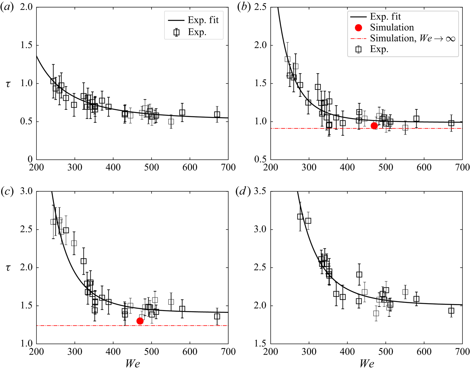
Figure 16. Breakup time dependence on the Weber number. The error bars indicate the time difference between subsequent snapshots before and after the breakup of the ligaments. (a) First breakup. (b) Second breakup. (c) Third breakup. (d) Fourth breakup.

A comparison with our simulations in figure 16 shows that the first and second breakup times in the simulation agree well with the experimental observations for the second and third breakup for both the $We=470$ and $We \to \infty$ simulations. Hence, it appears that our simulation cannot capture the first breakup in the experiment. This is due to the fine-scale nature of the first breakup, which our simulations are not able to resolve. In fact, from our experiments we measure ligament thicknesses during the first breakup ranging from 10 to 40 $\mathrm {\mu }$m, which corresponds to a resolution between $\sim$2–7 grid cells for these ligaments in our simulations. Nonetheless, the agreement of subsequent breakup times further validates both the simulations as well as the post-processing methodology for the experiments.

The functional dependence of the breakup onset on the Weber number is estimated using a nonlinear least-square fit of the experimental data of the form $\tau \approx a We ^b+c$ and plotted alongside the measurements in figure 16. The fitting coefficients are reported in table 1, which reveal a similar functional dependence for all breakup times. In particular, the similar exponents $a$ and constant difference between the offsets $c$ for all breakups reveal an approximately constant frequency between the breakups. This suggests that only the initial onset of the breakup is a function of the Weber number, whereas the breakup and its frequency are independent of capillary effects. Put differently, surface tension seems to delay the onset of the initial ligament shedding but does not affect the frequency of the recurrent shedding. Hence, these curves can be collapsed when shifted by $c$, which is reported in figure 17. The fit suggests that the breakup onset scales with $\tau \sim We ^{-4}$.

Figure 17. Collapse of all breakup times when shifted by their asymptotic breakup time. The least-square fit suggests $\tau \sim We ^{-4}$.

Table 1. Fitting coefficients for a nonlinear least-square fit of the form $\tau \approx a We ^b+c$. The confidence interval for all fitting coefficients is 0.95.

We conjecture that the breakup frequency is dominated by aerodynamic effects only. Such effects are dominant in the initial stages of the droplet deformation and previous studies of aerobreakup have shown a similar drag coefficient to that of a flow past a sphere (see, e.g. Meng & Colonius Reference Meng and Colonius2018). In our case, it is instructive to evaluate the Strouhal number $St={fD}/{U}$ for the observed breakups. However, the characteristic length scale, associated with the deforming and disintegrating droplet and its wake, is a priori not clear.To that end, in figure 18, we plot the evolution of the droplet core diameter throughout the breakup process for all experimental runs with Weber numbers in the range of $We =[200, 700]$. The diameter is measured directly from the shadowgraphs and defined as the maximum extent of the coherent liquid body of the droplet. Remarkably, the diameter evolution is independent of the Weber number and the droplet expands up to twice the size of its initial diameter for all experiments. Note that, at later stages for $\tau >1$, the core diameter decreases due to shedding and $D<2D_0$ but the small-scale structures and mist shed form the droplet, yielding an effective diameter which is larger than the diameter of the droplet core as plotted on figure 18. Hence, the maximum droplet diameter $D_m= 2D_0$ as a characteristic length scale seems to be the natural choice for reduction of the breakup frequency. This yields a mean Strouhal number of $St \approx 0.217$ when using all experimental data. Using the fitted data, one similarly obtains $St \approx 0.18$. Both frequencies agree well with what is observed for the flow past a rigid sphere (see, e.g. Achenbach Reference Achenbach1974; Kim & Durbin Reference Kim and Durbin1988; Sakamoto & Haniu Reference Sakamoto and Haniu1990). This suggests that the recurrent breakup is indeed induced by classical vortex shedding.

Figure 18. Diameter evolution for Weber numbers in the range $We =[200, 700]$.