


1. Introduction
Typical particle suspensions include flows in biomass combustors containing fuel particles, sandstorms, and tap water laden with tiny plastic particles. Usually, the Reynolds number of particle-laden flows is high in industry and nature, often associated with solid walls. Thus it is of great importance to understand the translation and clustering of particles in wall turbulence, especially at high Reynolds numbers (Eaton & Fessler Reference Eaton and Fessler1994; Balachandar & Eaton Reference Balachandar and Eaton2010).
It is widely observed that preferentially, particles migrate towards the wall and distribute non-uniformly in the vicinity of walls in turbulence (Fessler, Kulick & Eaton Reference Fessler, Kulick and Eaton1994; Marchioli et al. Reference Marchioli, Soldati, Kuerten, Arcen, Tanière, Goldensoph, Squires, Cargnelutti and Portela2008; Fong, Amili & Coletti Reference Fong, Amili and Coletti2019). Caporaloni et al. (Reference Caporaloni, Tampieri, Trombetti and Vittori1975) and Reeks (Reference Reeks1983) uncovered the turbophoresis mechanism that particles tend to drift towards the low turbulence intensity regions and explained the near-wall accumulation through analysing the translation equation of a particle. McLaughlin (Reference McLaughlin1989) performed a direct numerical simulation (DNS) of turbulent channel flow with particles and showed that particles aggregate into elongated clusters in low-speed streaks near the wall. Accumulation of particles in near-wall low-speed streaks hinders the particle transport in the streamwise direction (Eaton & Fessler Reference Eaton and Fessler1994). Rouson & Eaton (Reference Rouson and Eaton2001) found that particles with Stokes numbers scaled by the Kolmogorov time scale of the order of unity tend to concentrate into longitudinal bands in a turbulent channel flow at  $Re_\tau =180$, while larger inertia particles distribute randomly, suggesting that clustering is associated with some specific scales of flow motion. Marchioli & Soldati (Reference Marchioli and Soldati2002) found that the transport of particles is driven by near-wall sweeps and ejections in a low-Reynolds-number channel flow. The existence of quasi-streamwise vortices prevents near-wall particles from escaping to the outer layer region, resulting in near-wall high concentration. A similar mechanism was later confirmed by Picano, Sardina & Casciola (Reference Picano, Sardina and Casciola2009) in turbulent pipe flows. The streamwise length of particle streaks for intermediate inertial particles is longer than that of low-speed flow streaks. The spanwise spacing of particle streaks is approximately
  $120$ (
 $160$) viscous length units in turbulent channel (pipe) flows (Sardina et al. Reference Sardina, Picano, Schlatter, Brandt and Casciola2011). Moreover, Sardina et al. (Reference Sardina, Schlatter, Brandt, Picano and Casciola2012) showed that the streamwise length of these particle streaks is around 500–1000 viscous units. They also revealed that clustering near the wall is most prominent for particles with viscous Stokes number around 10–50, and the corresponding response time is of the same order of magnitude as the Kolmogorov time scale in the buffer layer (
 $\approx$ 5–10).
The dynamics of particles are influenced by turbulent coherent structures, which are multi-scale and contain a large proportion of the total kinetic energy in the turbulence field, especially at high Reynolds numbers (Balakumar & Adrian Reference Balakumar and Adrian2007). Turbulent structures like low- and high-speed flow regions in the logarithmic layer could be extremely long with meandering features (Hutchins & Marusic Reference Hutchins and Marusic2007a). However, due to the limitation of experiment facilities and computational capability, a number of previous studies on wall-bounded turbulence laden with particles are confined to relatively low Reynolds numbers. The segregation between small- and large-scale motion is not evident in turbulent channel flows at a low Reynolds number, while large-scale motions are more outstanding in turbulent Couette flows at a similar  $Re_\tau$. Therefore, Bernardini, Pirozzoli & Orlandi (Reference Bernardini, Pirozzoli and Orlandi2013) compared particle distributions in a turbulent Poiseuille flow and in a turbulent Couette flow to investigate the role of large-scale structures in the Couette flow. Large-scale particle streaks, with larger streamwise length and spanwise spacing than the near-wall small-scale streaks in the turbulent Poiseuille flow, are observed in the Couette flow, attributed to the presence of large-scale structures. Bernardini (Reference Bernardini2014) found that the turbophoretic drift of particles with intermediate inertia tends to be independent of the large-scale outer motion, while large inertial particles responded mainly to the outer-layer structure in channel flows at
  $Re_\tau$ up to
  $1000$. Recently, Wang & Richter (Reference Wang and Richter2019) performed two-way coupled DNS of particle-laden channel flows at
  $Re_\tau =550$ and
  $950$. They found that low- and high-inertia particles enhance very-large-scale motions (VLSMs). Distinct clustering structures in the outer layer are found for high-inertia particles. They later showed that particles of different inertia react to buffer-layer large-scale motions (LSMs) and VLSMs in distinct ways (Wang & Richter Reference Wang and Richter2020). Jie, Andersson & Zhao (Reference Jie, Andersson and Zhao2021) found that the clustering of particles is affected by the quiescent core region in a turbulent channel flow at
  $Re_\tau =600$. The coherent clusters of inertial particles have drawn attention in the community. Baker et al. (Reference Baker, Frankel, Mani and Coletti2017) showed that coherent clusters tend to sample high-strain and low-vorticity regions, and align themselves with the local vorticity vector. Oujia, Matsuda & Schneider (Reference Oujia, Matsuda and Schneider2020) found that the divergence of particles is most evident in cluster regions and enhances when the Stokes number increases. A recent experimental study in turbulent boundary layers at friction Reynolds number up to
  $Re_\tau =19000$ (Berk & Coletti Reference Berk and Coletti2020) showed that the particles are often found in ejection events for a wide range of wall-normal distance
  $y^+$ and Stokes number. Interestingly, Scherer et al. (Reference Scherer, Uhlmann, Kidanemariam and Krayer2022) recently studied the formation of subaqueous sediment ridges on a sediment bed at
  $Re_\tau \in [250, 850]$ and found that the ridges tend to appear in regions below the large-scale low-speed flow streaks.
On the one hand, the clustering and transport of particles are affected by turbulent structures (Bernardini et al. Reference Bernardini, Pirozzoli and Orlandi2013; Wang & Richter Reference Wang and Richter2020; Jie et al. Reference Jie, Andersson and Zhao2021). On the other hand, it is shown by spectral analysis that VLSMs make a significant contribution to both Reynolds shear stress and turbulent kinetic energy, and the significance grows with increasing Reynolds number (Balakumar & Adrian Reference Balakumar and Adrian2007; Smits, McKeon & Marusic Reference Smits, McKeon and Marusic2011). Therefore, we expect that the effects of large-scale motions/structures on particle behaviours become increasingly prominent and important at high Reynolds numbers. However, studies about the effects of turbulent structures in wall turbulence on particle dynamics are still rare, especially at relatively high  $Re_\tau$. The main goal of the present work is to study the near-wall accumulation of particles and the correlation between particle distribution and the surrounding turbulent structures at high Reynolds numbers. Section 2 provides numerical details of the simulations. Instantaneous and statistical results are provided and discussed in § 3, and conclusions are drawn in § 4.
2. Method
The incompressible Newtonian fluid flows considered in the present study are governed by the mass conservation and Navier–Stokes equations:
 \begin{equation} \left.\begin{gathered} \frac{\partial u_i}{\partial x_i} =0, \\ \frac{\partial u_i}{\partial t} + u_j\,\frac{\partial u_i}{\partial x_j} ={-}\frac{1}{\rho}\,\frac{\partial p}{\partial x_i} + \nu\,\frac{\partial^2 u_i}{\partial x_j\, \partial x_j} , \end{gathered}\right\}\end{equation}
where  $u_i$ is the velocity component in the
  $x_i$ direction of an inertial Cartesian frame, and
  $p$ denotes the pressure. Air is considered as the fluid phase with kinematic viscosity
  $\nu = 1.364\times 10^{-5}\ \textrm {m}^2\ \textrm {s}^{-1}$ and density
  $\rho = 1.225\ \textrm {kg}\ \textrm {m}^{-3}$. The equations are solved with periodic boundary conditions in the homogeneous streamwise (
 $x$) and spanwise (
 $z$) directions, and no-slip/no-penetration conditions at both walls (
 $y=0,2h$, where
  $h$ is the half-height of the channel). Physical variables are labelled by a superscript
  $+$ after being normalized by the viscous units such as the time unit
  $\tau _\nu = \nu /u_\tau ^2$ and length unit
  $\delta _\nu = \nu /u_\tau$. The friction velocity is
  $u_\tau = \sqrt {\tau _w/\rho }$, where
  $\tau _w$ denotes the average wall shear stress. A pseudo-spectral method is adopted in the streamwise and spanwise directions, while a second-order finite difference scheme is employed in the wall-normal direction. Utilizing a second-order Adams–Bashforth scheme for time evolution, four turbulent channel flows with different
  $Re_\tau = u_\tau h/\nu$ ranging from
  $600$ to
  $2000$ are simulated as summarized in table 1.
Table 1. Summary of simulation parameters, where  $\Delta y_w^+$ and
  $\Delta y_c^+$ denote the grid spacing at the wall and the centreline, respectively, and
  $N_p$ is the particle number of each type. Particles with
  $St_\nu =0$ are tracers.

The turbulent channel flows are suspended with spherical point particles, which are tracked individually using a Lagrangian approach. The mass of a particle is  $m = 4{\rm \pi} a^3 \rho _p /3$, where
  $\rho _p$ is the density of particle and
  $a$ represents the radius. The particles are sub-Kolmogorov, namely sufficiently small, and much heavier than the fluid so that we consider only the Stokes drag force. Moreover, a semi-empirical correction for Stokes drag (Schiller & Naumann Reference Schiller and Naumann1933) is adopted to guarantee a reasonable drag force, while the average particle Reynolds numbers
  $Re_p = 2a\lVert \boldsymbol{ {u}} - \boldsymbol{ {v}}\rVert /\nu$ of all cases are smaller than 1 in the present study (not shown). A sufficiently dilute suspension of sub-Kolmogorov particles is considered so that it is justified to adopt the assumption of one-way coupling without including a feedback force term in (2.1). Gravity is neglected for the sake of highlighting the effects of particle inertia and turbulent structures. The particle Froude numbers
  $Fr_p = U_b / g \tau _p$ considered in the present study are all larger than
  $1$, where
  $U_b$ is the bulk velocity of the channel flow, supporting that the gravity effect is negligible compared with the effect of the bulk motion of fluid flow (Milici et al. Reference Milici, Marchis, Sardina and Napoli2014). One should note that the gravity effect in the wall-normal direction might be non-negligible compared to the turbophoresis effect, even when the settling number is smaller than one (Bragg, Richter & Wang Reference Bragg, Richter and Wang2021). All the particles considered in the present study have a normalized diameter
  $D^+=0.6<1$, which leads the magnitude of the Saffman lift force to be much smaller than the Stokes drag force (Costa, Brandt & Picano Reference Costa, Brandt and Picano2020). Therefore, we neglect the lift force in the present study, while one should note that the effect of the wall-normal lift force may arise for the particles embedded in the sublayer, where these particles normally stay for a long time. The governing equations of particle motion are
 \begin{equation} \left.\begin{gathered} v_i = \frac{\mathrm{d}\kern0.7pt x_i}{\mathrm{d} t}, \\ \frac{\mathrm{d} v_i}{\mathrm{d} t} = \frac{1}{\tau_p}\,(u_{p,i}-v_i)(1+0.15Re_p^{0.687}), \end{gathered}\right\}\end{equation}
where  $u_{p,i}$ is the velocity of fluid at particle position, and
  $\tau _p = 2a^2 \rho _p / 9 \rho \nu$ is the particle response time. In our study, three different Stokes numbers are considered, and their expressions are given as
 \begin{equation} \left.\begin{gathered} \text{viscous Stokes number }St_\nu = \tau_p /\tau_\nu, \\ \text{Kolmogorov Stokes number }St_\eta = \tau_p / \tau_\eta, \\ \text{structure-based Stokes number }St_{Q^-} = \tau_p / T_{Q^-}, \end{gathered}\right\} \end{equation}
non-dimensionalized by the viscous time unit  $\tau _\nu$, the local Kolmogorov time unit
  $\tau _\eta$ and the lifetime of a typical
  $Q^-$ structure
  $T_{Q^-}$ (Lozano-Durán & Jiménez Reference Lozano-Durán and Jiménez2014), respectively. The lifetime of the
  $Q^-$ structures and the structure-based Stokes number will be discussed in detail in § 3.
The collisions are fully elastic between the solid walls and particles, while periodic boundary conditions are employed in the spanwise and streamwise directions. Particles are released randomly into the domains after the flows are statistically fully developed at  $t^+ = 0$. Particle number and Stokes numbers are given in table 1. Since channels S6h, S1k and S2k contain large-inertia particles with
  $St_\nu >200$, the following statistical results are collected mainly from these channel flows in the time windows
  $t^+ = 2337.1 - 5842.6$,
  $t^+ = 2502.6 - 5005.1$ and
  $t^+ = 2570.3 - 4443.0$, respectively. Please note that the statistics of particle concentration in the wall-normal direction are not yet statistically steady, which requires a long time computation (Bernardini Reference Bernardini2014). However, qualitatively the conclusions of the present cases are valid since the focus is on understanding the formation of near-wall particle streaks and the interaction between inertial particles with a certain Stokes number and the primary turbulent structures, to which these particles respond most quickly and efficiently and thus form near-wall streaky patterns in a short time. Concerning the time window for obtaining statistics adopted in the present study, particles are allowed to travel in the domain during
  $O(10)$ times of
  $T_{Q^-(LS)}$, which is the average lifetime of the large-scale
  $Q^-$ structure. According to the results shown in the following section, the time window chosen in the present study is enough for the particles to form long streaks under the influence of primary
  $Q^-$ structures.
3. Results
3.1. Particle streaks
First, an instantaneous streamwise–spanwise plot of two-dimensional Voronoï cells is shown in figure 1(a) for  $St_\nu =200$ particles at
  $y^+ \in [2,4]$. The Voronoï tessellation is a method to identify and quantify clustering of particles (Monchaux, Bourgoin & Cartellier Reference Monchaux, Bourgoin and Cartellier2012). Each particle has a unique Voronoï cell, which contains the area that is closer to the particle than to any others. Hence the area of a Voronoï cell reflects the local clustering degree directly. The Voronoï areas are all normalized by the mean value in the selected plane. Note that only the Voronoï cells with a normalized area smaller than unity are shown, indicating the regions where particles are preferentially accumulated. Several particle streaks are present in the vicinity of the wall, with the streamwise and spanwise scales much larger than those well-observed small-scale ones in low-Reynolds-number wall-bounded turbulence, typically for
  $St_\nu \approx 30$ particles (Sardina et al. Reference Sardina, Picano, Schlatter, Brandt and Casciola2011). These large-scale particle streaks are straight, and long enough to penetrate the whole computational domain with streamwise length
  $L_x^+ \approx 25\,133$, while the length of conventional particle streaks observed in earlier studies is only around 500–1000 viscous units (Sardina et al. Reference Sardina, Schlatter, Brandt, Picano and Casciola2012). The corresponding instantaneous streamwise velocity fluctuations at
  $y^+ \approx 125$ are shown in figure 1(b), which reveals the correlation between large-scale particle streaks and large-scale motions of the turbulence at
  $y^+ = 3.9 \sqrt {Re_\tau } \approx 123.3$, namely the middle of the log layer (Mathis, Hutchins & Marusic Reference Mathis, Hutchins and Marusic2009). As shown in figure 1(b), the particle streak at
  $z^+ \approx 2000$ is related to the low-speed flow streak at
  $z^+ \approx 2000$, both of which are elongated throughout the computational domain at the same spanwise location.

Figure 1. (a) Instantaneous streamwise–spanwise plot of two-dimensional Voronoï areas of aggregated particles with  $St_\nu =200$ at
  $y^+\in [2,4]$. The pictured Voronoï cells all have normalized areas smaller than
  $1$, indicating the clustering region of particles. (b) The corresponding instantaneous contour of the streamwise fluid velocity fluctuation
  $u_1'$ at
  $y^+ \approx 125$ in channel L1k.
The flow streaks near walls have been investigated in earlier studies of experiments and simulations (Kline et al. Reference Kline, Reynolds, Schraub and Runstadler1967; Kim & Adrian Reference Kim and Adrian1999). The spanwise spacing of the near-wall fluid velocity streaks is around 80–120 viscous units and is almost Reynolds-number-independent, while the streamwise length of these streaks can be larger than  $1000\delta _\nu$. In addition to the near-wall streaks, very large-scale motions with the largest scale of the order of the streamwise length of the domain have been observed in pipe flows (Kim & Adrian Reference Kim and Adrian1999; Monty et al. Reference Monty, Hutchins, Ng, Marusic and Chong2009). Balakumar & Adrian (Reference Balakumar and Adrian2007) adopted a wavelength of
  $3$ pipe radii as a nominal criterion to distinguish the LSMs and VLSMs. Very long meandering low- and high-speed flow streaks are also observed in the logarithmic regions of wall-bounded turbulence (Hutchins & Marusic Reference Hutchins and Marusic2007a). The length of these streaks can exceed
  $20\delta$, and penetrate throughout the domain, consistent with the present observations in figure 1(b).
Figure 1 shows that large-scale particles streaks are prominent near the wall in the ‘footprint’ of flow structures in the logarithmic regions. In figures 2 and 3, we choose the near-wall regions to examine the particle distribution since the clustering pattern of particles is most observable there. The autocorrelation of particle concentration fluctuation is computed to quantify the clustering of particles in the viscous sublayer ( $0 < y^+ <5$), which is defined as
 \begin{equation} R_{cc}(\Delta z^+) = \frac{\langle c'(x^+,z^+)\,c'(x^+,z^+{+}\Delta z^+)\rangle}{\langle c'(x^+,z^+)\,c'(x^+,z^+) \rangle}, \end{equation}
where  $c'$ is the particle concentration fluctuation computed in equally-spaced subdivided bins with streamwise size
  $\Delta x^+$ and spanwise size
  $\Delta z^+$. The autocorrelation coefficients
  $R_{cc}$ in channels S6h, S1k and S2k are shown in figure 2. The size of the box adopted to compute the local concentration
  $c$ is given by
  $\Delta x^+ = 300$,
  $\Delta z^+ = 10.5$ and
  $0 < y^+ < 5$ in channels S6h and S1k. The streamwise length of small-scale particle streaks is of the magnitude of
  $10^3$ viscous units according to Sardina et al. (Reference Sardina, Schlatter, Brandt, Picano and Casciola2012), while the spanwise spacing between these structures is around
  $120$ inner units in channel flows (Sardina et al. Reference Sardina, Picano, Schlatter, Brandt and Casciola2011).
  $\Delta x^+$ is chosen to be less than the mean length of particle streaks, and
  $\Delta z^+ = 10.5$ is small enough to distinguish adjacent particle streaks in the box-counting approach. A larger box with
  $\Delta x^+ = 900$,
  $\Delta z^+ = 21.0$ and
  $0 < y^+ < 20$ is employed in channel S2k to ensure enough particles for obtaining smooth statistics in the boxes since the size is smaller than those in channels S6h and S1k if normalized by the outer scales. A box of the same size as that in channels S6h and S1k has been adopted to compute the autocorrelation coefficients in channel S2k (not shown), and it is found that the peaks of the coefficients are still present for different Stokes numbers although the curves are not as smooth as those in figure 2(c). The correlation peak values are sensitive to the bin size but the peak position is almost bin-size independent (Sardina et al. Reference Sardina, Picano, Schlatter, Brandt and Casciola2011). The large-scale particle streaks are very long and straight as shown in figure 1(a), hence it is reasonable to adopt larger boxes in channel S2k and it does not change our further conclusions.

Figure 2. Autocorrelation coefficients of particle concentration fluctuation  $c'$ at (a)
  $Re_\tau =600$, (b)
  $Re_\tau =1000$, and (c)
  $Re_\tau =2000$.

Figure 3. Spectrum of  $R_{cc}$ versus the spanwise wavelength
  $\lambda _z^+$ in channel (a1) S6h, (b1) S1k, (c1) S2k. Corresponding mean values of
  $S(R_{cc})$ in sections
  $[100,200]$ and
  $[0.7,1.5]\times h^+$ in channel (a2) S6h, (b2) S1k, (c2) S2k.
In figure 2, the particles at  $Re_\tau =600$ are divided into three groups: tracer-like and ballistic particles with
  $St_\nu =0,1000$ in figure 2(a1); relatively light particles with
  $St_\nu =10,30,50$ in figure 2(a2); relatively heavy particles with
  $St_\nu =150 - 300$ in figure 2(a3). There is no obvious valley and secondary peak for tracer-like and ballistic particles in figure 2(a1), since their distribution is nearly random and no obvious particle streaks are formed. However, the effects of two different scales are observed for the other two groups. Small-scale particle streaks are found in figure 2(a2). The first valley shows up around
  $\Delta z^+ \approx 50$, indicating the spacing of small-scale particle streaks about
  $\Delta z^+ \approx 50\times 2 = 100$, which is consistent with the findings by Sardina et al. (Reference Sardina, Picano, Schlatter, Brandt and Casciola2011). On the other hand, a large-scale valley resides around
  $\Delta z^+ \approx 300$, as shown in figure 2(a3). Two prominent large-scale peaks are present at
  $\Delta z^+ \approx 500$ and
  $800$, which are both around
  $\Delta z \approx h$ in the outer unit.
Figure 2(b) displays the correlation coefficients of particles in channel S1k, showing a multi-scale feature similar to that in figure 2(a). A clearly small-scale valley of  $R_{cc}$ in figure 2(b2) resides around
  $\Delta z^+ \approx 50$ for relatively light particles with
  $St_\nu =10$,
  $30$ and
  $50$, which form small-scale particle streaks. Large-scale valleys of
  $R_{cc}$ are shown at
  $\Delta z^+ \approx 500 - 600$ in figure 2(b3), suggesting that large-scale streaks are more obvious for relatively heavy particles with
  $St_\nu =150 - 300$. The spanwise spacing of large streaks is also around
  $\Delta z = h$ in this case. As inertia keeps increasing, the large-scale valleys/peaks are diminished since larger inertia particles ignore fluctuations of small scales and thus distribute randomly (figure 2b1). The correlation coefficients of particles in channel S2k at
  $Re_\tau = 2000$ are shown in figure 2(c). Please note that the magnitudes of the autocorrelations are relatively smaller than those in figure 2(a,b). Statistically, the speed of particle accumulation in the wall region depends on the flow Reynolds number (Bernardini Reference Bernardini2014), and the wall-normal accumulation is slower for the higher
  $Re_\tau$ case. It leads to smaller
  $R_{cc}$ values in the
  $Re_\tau =2000$ case at a similar
  $t^+$. Small-scale streaks, suggested by the local valleys in figure 2(c2) around
  $\Delta z^+ \approx 50$, are observable for the particle group with intermediate inertia (
 $St_\nu =10 - 50$). The autocorrelation is nearly zero for tracer and ballistic particles as
  $St_\nu =0$ and
  $1000$ in figure 2(c1). Local peaks are present in figure 2(c3) at
  $\Delta z^+=1500 - 2000$, indicating the existence of large-scale particle streaks with a spanwise spacing roughly 1500–2000, while the peaks are not as prominent as those shown in figure 2(a3,b3). The local peaks could be more observable if the statistical box size is extended further (not shown) while the characteristic large-scale wavelength of the autocorrelation
  $R_{cc}$ curves remains the same. However, the following analysis of the spectrum of
  $R_{cc}$ reveals that there are also large-wavelength components of
  $R_{cc}$ in the S2k case.
Figure 2 indicates multi-scale effects of underlying turbulence on particle distributions and shows that particles with different  $St_\nu$ form the streaks with different spanwise spacing. To reveal the characteristic spacings of streaks and to find out the corresponding Stokes numbers, the spectrum of the particle concentration fluctuation,
  $S(R_{cc})$, is computed and shown versus the spanwise wavelength
  $\lambda _z^+$ in figure 3. As pointed out by Sardina et al. (Reference Sardina, Picano, Schlatter, Brandt and Casciola2011), small-scale particle streaks have typical spanwise spacing
  $\varDelta _z^+ \approx 120$. In the present study, the characteristic spanwise spacing of large-scale particle streaks is about
  $h$ (see figure 2), which, in our view, is related to the spanwise spacing of the underlying flow streaks. Hutchins & Marusic (Reference Hutchins and Marusic2007a) observed very-long meandering streaks in the logarithmic region and showed that the spanwise spacing between adjacent streaks is roughly
  $\Delta z \approx \delta$ through the spanwise two-point correlations of the streamwise velocity fluctuation. As indicated by figure 3(a1), the spectrum values
  $S(R_{cc})$ of particles with intermediate Stokes number (
 $St_\nu =10,30,50$) are higher than those of others at the spanwise wavenumber
  $\lambda _z^+$ around
  $120$, whereas spectrum values of
  $St_\nu =10 - 50$ particles are lower than those of high-inertia particles with
  $St_\nu =100 - 300$. As for tracers (
 $St_\nu =0$) and heavy ballistic particles (e.g.
  $St_\nu =1000$), there is no prominent spectrum component at almost all wavelengths
  $\lambda _z^+$ compared to the intermediate inertial particles. The local maximum around
  $\lambda _z^+ \approx 120$ is related to the small-scale particle streaks with mean spacing
  $\varDelta _z^+ \approx 120$, while the local maximum of wavelength
  $\lambda _z$ around
  $h$ is associated with the large-scale particle streaks shown in figure 1(a) and revealed by figure 2(c). Similar local peaks around both
  $\lambda _z^+ \approx 120$ and
  $\lambda _z \approx h$ are also present in figure 3(b1,c1). The peak around
  $\lambda _z^+ \approx 1500$ in figure 3(c1) corresponds to the peak at
  $\Delta z^+ = 1500 - 2000$ in figure 2(c3). For the purpose of evaluating quantitatively the significance of particle streaks at various Stokes numbers, two intervals of the wavelength are chosen to compute the averaged spectrum values
  $S(R_{cc})$. One interval is
  $\lambda _z^+ \in [100,200]$, as shown between the vertical black dotted lines in the left-hand panels (a1,b1,c1) of figure 3, while the other is
  $\lambda _z \in [0.7,1.5]\times h$ between the vertical blue dotted lines. The choice of lower and upper limit values (
 $0.7h$ and
  $1.5h$) does not affect the following qualitative conclusions. The average spectrum values in the two intervals are shown in the right-hand panels (a2,b2,c2) of figure 3, in which the peaks of the black dashed lines all locate at
  $St_\nu =30$, and the secondary ones are at
  $St_\nu =10$. It suggests that the Stokes number of the particles forming the most prominent small-scale streaks is
  $St_\nu \approx 30$ (
 $10< St_\nu <50$ in the present study), which keeps almost unchanged as
  $Re_\tau$ is up to
  $2000$. Nevertheless, the locations of peaks for the blue lines vary. A Gaussian fitting method is adopted to identify the peaks of the blue lines in figure 3(a2,b2,c2). The corresponding peaks are found to locate at
  $St_\nu =136.07,155.75,250.15$ for channels S6h, S1k and S2k, respectively. These Stokes numbers are Reynolds-number-dependent and are classified as prominent Stokes numbers (
 $St_\nu =St_{\nu (pro)} = \tau _{p(pro)}/\tau _\nu$) hereinafter. Here,
  $\tau _{p(pro)}$ is the corresponding particle response time. The
  $St_{\nu (pro)}$ value increases as
  $Re_\tau$ grows, and seems to be proportional to the scale of the underlying flow structures.
3.2. The effect of large scale motion on particle streaks
Inspired by the correlation between large-scale particle streaks in the viscous sublayer and large-scale low-speed motion in the middle of the log layer, conditional averages are further performed to investigate the the mechanism of formation of the large-scale particle streaks. To quantitatively determine the centre of the large-scale particle streaks in an instantaneous field, particles inside a three-dimensional subdomain with streamwise length  $\Delta x^+ = 40$, wall-normal location in
  $0< y^+ <5$, and spanwise location in
  $0 \leqslant z^+ \leqslant L_z^+$ are extracted to draw the kernel density estimation (KDE) of particle distribution with kernel width
  $b^+ = 100$. The peaks of the KDE are then identified. The peaks’ corresponding spanwise location
  $z^+$ is treated as the centre of large-scale particle streaks in the subdomain, labelled as
  $\Delta z^+ = 0$ later in the figures. Afterwards, a conditional average along the particle streaks is calculated based on the identified locations. The conditional average of natural logarithm of particle concentration
  $\ln (c^+)$ is calculated and shown in figure 4(a) for particles with
  $St_\nu =200$ in channel S1k. The accumulation of particles around
  $\Delta z^+ \approx 0$ denotes the large-scale particle streaks. Note that the contours around
  $\Delta z^+ \approx 0$ are bulgy toward the outer region even at
  $y^+\approx 100$, which indicates that the large-scale particle streaks can reach the logarithmic region, whereas particle concentrations are relatively lower, around
  $\Delta z^+ \approx \pm 300$ compared to that about
  $\Delta z^+ \approx 0$ at the same
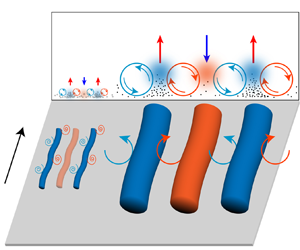
  $y^+$ plane. The conditional-averaged streamwise velocity fluctuations sampled in the same time window are shown in figure 4(b), where the background colour represents the streamwise velocity fluctuations and the vectors (white arrows) show the relative magnitude and direction of the velocity projection in the plane. The blue region around
  $\Delta z^+ \approx 0$ represents a large-scale low-speed streak of fluid flow. Two large-scale high-speed regions, coloured in red, are present around the low-speed streak. The side-by-side high- and low-speed regions indicate the existence of a clockwise vortex (
 $\Delta z^+ \approx 150$) and an anticlockwise one (
 $\Delta z^+ \approx -300$), which are visualized by the vectors. Moreover, the upward flow in the blue region denotes a large-scale ejection (
 $Q2$) event while the downward flow in the red areas represents two large-scale sweep (
 $Q4$) events.
  $Q1$ events denote
  $u'>0, v'>0$,
  $Q2$ events denote
  $u'<0, v'>0$,
  $Q3$ events have
  $u'<0, v'<0$ and
  $Q4$ events have
  $u'>0, v'<0$ hereinafter. According to figure 4, we find that particles are transferred by large-scale
  $Q2$,
$Q2$,  $Q4$ events and the two large vortices, and eventually accumulate around the large-scale low-speed regions about
  $\Delta z^+ \approx 0$. This finding is consistent with the experimental observation in high-
 $Re$ wall turbulence by Berk & Coletti (Reference Berk and Coletti2020), who found that inertial particles preferentially stay in the regions of negative streamwise fluctuations, especially in
  $Q2$ events, and this tendency is observed for a wide range of Stokes number, indicating a multi-scale nature of preferential concentration. The formation of small-scale streaks has been studied by Marchioli & Soldati (Reference Marchioli and Soldati2002). But in contrast to these small-scale streaks, the time and length scales of particle streaks and flow vortices observed in figure 4 are both much larger. In our view, both small- and large-scale particle streaks are related to the counter-rotating vortices and
  $Q2$,
$Q2$,  $Q4$ events, but the particles of different inertia respond to the flow motions of different scales.

Figure 4. Conditional average of (a) particle concentration  $\ln (c^+)$ (base
  $e$), (b) the surrounding flow field along the large-scale particle streaks for
  $St_\nu =200$ particles in channel S1k.
3.3. Relationship of the time scale between large-scale flow structures and particles
Two scales of particle streaks are observed in figure 2, namely small-scale ones of  $St_\nu \approx 30$ particles and large-scale ones, such as
  $St_\nu \approx 150$ particles at
  $Re_\tau =1000$. The small-scale ones are most prominent when
  $St_\nu \approx 30$, which seems independent of
  $Re_\tau$. We therefore infer that the formation of small-scale particle streaks is governed mainly by the near-wall structures, whose time scale is nearly constant with increasing
  $Re_\tau$, while the large-scale streaks are induced mainly by the structures of turbulence whose time scale increases when
  $Re_\tau$ grows.
As shown in figure 4, particle translation in the wall-normal direction is affected by sweep ( $Q4$) and ejection (
 $Q2$) events. Thus it is reasonable to study the correlation between particle streaks and
  $Q2$,
$Q2$,  $Q4$ structures (i.e.
  $Q^-$ structures). We notice that the time-resolved evolution of coherent structures has been studied systemically by Lozano-Durán & Jiménez (Reference Lozano-Durán and Jiménez2014). They tracked the coherent structures of quadrant events (
 $Q1$ to
  $Q4$) and evaluated the lifetime of structures. The quadrant events satisfy
 \begin{equation} {} | u'(\boldsymbol{x})\,v'(\boldsymbol{x})| > H\,u'_{rms}(y)\,v'_{rms}(y), \end{equation}
where  $-u'(\boldsymbol {x})\,v'(\boldsymbol {x})$ is the instantaneous tangential Reynolds stress, and
  $H=1.75$. Regions with Reynolds stress satisfying (3.2) are identified first and then classified into different structures based on the connectivity of the points. The
  $Q^-$ structures are different objects with different characteristic heights and time scales. Lozano-Durán & Jiménez (Reference Lozano-Durán and Jiménez2014) found that the
  $Q^-$ in the buffer layer have a lifetime of
  $30$ in viscous units, and the lifetime of the primary large-scale
  $Q^-$ is proportional to the local eddy-turnover time
  $T^+ \approx l_y^+$, where
  $l_y^+$ is the mean height of large-scale structures. Therefore, the lifetime of large-scale structures can be estimated by the typical height of structures (
 $T^+ \approx l_y^+ \approx y_{LS}^+$).
Furthermore, Marusic, Mathis & Hutchins (Reference Marusic, Mathis and Hutchins2010) showed that the inner peak in the premultiplied energy spectra of streamwise velocity fluctuation is around  $y^+ \approx 15$, namely in the buffer layer, while the outer peak locates around the middle of the log layer, where
  $y_{LS1}^+ \approx 3.9\sqrt {Re_\tau }$. It suggests that large-scale motions of this magnitude are most prominent. Therefore, the time scale of the large-scale structures can be estimated as
  $T_{LS}^+ \approx y_{LS1}^+ = 3.9 \sqrt {Re_\tau }$. On the other hand, since the particle translation is strongly associated with the
  $Q^-$ events, the lifetime of the
  $Q^-$ structures can be adopted to estimate
  $T_{LS}^+$. The wavenumber-premultiplied energy spectral densities
  $-k_z E_{u'v'}/u_\tau ^2$ of turbulent channel flows are computed as in figure 5 using data from an online database (Lee & Moser Reference Lee and Moser2015). Evident outer peaks appear when
  $Re_\tau$ is high enough, i.e.
  $Re_\tau =1000$,
  $2000$ and
  $5200$. The peaks are found to follow
  $y_{LS2}^+ \approx 0.25 Re_\tau$ in the
  $Re_\tau$ range up to
  $5200$ as indicated by the blue dash-dotted lines in figure 5. Thus the second estimation of the time scale of the large-scale structures is
  $T_{LS}^+ \approx y_{LS2}^+ \approx 0.25 Re_\tau$. The two estimations of the characteristic length scale of large-scale structures,
  $y_{LS1}^+ \approx 3.9\sqrt {Re_\tau }$ and
  $y_{LS2}^+ \approx 0.25Re_\tau$, are both derived from the location of the outer peak in different premultiplied energy spectra. It is reasonable that their magnitudes are similar since they both represent the wall-normal characteristic height of the large-scale structures in the outer region.

Figure 5. Wavenumber-premultiplied energy spectral density  $-k_z E_{u'v'}/u_\tau ^2$ of turbulent channel flows at (a)
  $Re_\tau =550$, (b)
  $Re_\tau =1000$, (c)
  $Re_\tau =2000$, and (d)
  $Re_\tau =5200$. The horizontal black dashed lines denote
  $y_{LS1}^+ = 3.9\sqrt {Re_\tau }$, and the blue dash-dotted lines are
  $y_{LS2}^+ = 0.25Re_\tau$ (
 $y/\delta = 0.25$). Data are from an online database (Lee & Moser Reference Lee and Moser2015).
For the sake of analysing the change in  $St_{\nu (pro)}$ versus Reynolds number, the prominent Stokes numbers
  $St_{\nu (pro)}$ at three Reynolds numbers are shown in figure 6, together with two estimated lifetimes of large-scale
  $Q^-$ structures in turbulent channel flows. The black circles represent the particles with prominent Stokes numbers, which are identified by the peaks of the Gaussian fitting method in figure 3(a2,b2,c2). These particles tend to form the most prominent large-scale streaks. The black squares stand for the particles with
  $St_\nu =30$ that tend to aggregate into small-scale streaks. Two estimations of the height of large-scale structures are adopted in figure 6 through evaluating the location of the outer peak in a premultiplied energy spectrum. All
  $St_{\nu (pro)}$ dots are confined in the region between the two estimations. We conclude that
  $St_{\nu (pro)}$ keeps increasing with
  $Re_\tau$ in accordance with the lifetime of large-scale structures, which also grows when Reynolds number rises. The values between
  $3.9\sqrt {Re_\tau }$ and
  $0.25 Re_\tau$ can be used to estimate
  $St_{\nu (pro)}$ in the present
  $Re_\tau$ range.

Figure 6. Prominent Stokes numbers  $St_{\nu (pro)}$ at different
  $Re_\tau$ and two estimated lifetimes of large-scale
  $Q^-$ structures in turbulent channel flows. The black circles represent the particles with
  $St_\nu =St_{\nu (pro)}$ as defined in figure 3(a2,b2,c2). The black squares stand for the characteristic
  $St_\nu$ for small-scale streaks.
Generally, a particle is driven mainly by its surrounding flow, and the translation of particles in flow structures is then affected by the birth and death of the structures. Therefore, it is reasonable that the behaviours of particles are associated with the lifetimes of turbulent structures. The aforementioned results reveal that the primary small- and large-scale flow structures greatly affect the particle near-wall clustering, and therefore we propose a newly-defined Stokes number, the structure-based Stokes number ( $St_{Q^-} = \tau _p / T_{Q^-}$), scaled by the lifetime of typical flow structures of wall turbulence.
Typical  $St_\nu$ of small-scale particle streaks in the vicinity of walls is
  $St_\nu \approx 30$. It is a long-lasting puzzle that the strongest clustering in the vicinity of walls is shown at
  $St_\nu \approx 30$ at low
  $Re_\tau$, but no widely-accepted physical explanation is given. The structure-based Stokes number
  $St_{Q^-(BF)}$ based on the time scale of the buffer layer
  $Q^-$ is
  $St_{Q^-(BF)}= \tau _p / T_{Q^-(BF)}$. Since
  $T_{Q^-(BF)} \approx 30 \tau _\nu$, the structure-based Stokes number
  $St_{Q^-}$ of
  $St_\nu \approx 30$ particles is approximately unity, suggesting that the response times of these particles are comparable with the lifetime of the
  $Q^-$ in the buffer layer (BF indicates ‘buffer layer’). In our view, the underlying mechanism for the formation of large-scale particle streaks is similar to that for small-scale streak formation, while the large-scale particle streaks are induced by the
  $Q^-$ structures with large scales. Since the lifetime of these large-scale
  $Q^-$ is between
  $3.9\sqrt {Re_\tau }$ and
  $0.25Re_\tau$ (figure 6), the structure-based Stokes number of the particles with
  $St_\nu = St_{\nu (pro)}$ follows
  $St_{Q^-(LS)}= \tau _p(St_\nu = St_{\nu (pro)}) / T_{Q^-(LS)} \approx 1$. A simple linear fitting expression of
  $St_{\nu (pro)}$, based on the data points (circles in figure 6), is
 \begin{equation} St_{\nu (pro)} \propto 0.1 Re_\tau,\quad\text{or}\quad\tau_{p(pro)} \propto 0.1 \times \frac{h}{u_\tau}, \end{equation}
to roughly describe the relationship between the prominent Stokes numbers and Reynolds number (or the time scale of primary large-scale structures). However, in reality, such as in sandstorms, the upper limit of the particle Stokes number depends on the limits of density ratio and particle size. For instance, the Stokes number of PM10 particles is  $St_\nu = 260 - 1700$ in sandstorms (Wang, Gu & Zheng Reference Wang, Gu and Zheng2020). The effect of gravity will also show up if the particle size is sufficient large. Hence the predicted
  $St_{\nu (pro)}$ may be not in the range of realistic
  $St_\nu$ at
  $Re_\tau$ above
  $10^4$, and the gravity effect may play a role for large particles, which is not considered in the present work.
As a remark, to estimate the near-wall accumulation of particles in wall turbulence, the structure-based Stokes number proposed in this study performs better than the Kolmogorov–Stokes number. Small-scale clustering is most prominent for particles with Kolmogorov–Stokes number  $St_\eta = \tau _p / \tau _\eta \approx 1$ in homogeneous isotropic turbulence, where
  $\tau _\eta$ is the Kolmogorov time scale, while the wall-normal accumulation of particles is not well correlated with the Kolmogorov–Stokes number, which reflects only the effect of small-scale turbulence fluctuations. The Kolmogorov–Stokes number
  $St_\eta$ normalized by the Kolmogorov time scale
  $\tau _\eta (y^+)$ ranges from
  $3$ (near-wall region) to
  $30$ (central region) for the
  $St_\nu =30$ particles at
  $Re_\tau =1000$. Therefore, the
  $St_\eta$ for the particles of the strongest near-wall clustering with
  $St_\nu =30$ is always larger than
  $3$, which suggests that the Kolmogorov–Stokes number
  $St_\eta$ may not be a good criterion to estimate the near-wall accumulation of particles.
4. Conclusions
The accumulation of solid particles in turbulent channel flows has been studied numerically to investigate the geometrical features of different-scale particle streaks and the role of the flow structures that control the particle streaks at  $Re_\tau$ ranging from
  $600$ to
  $2000$, which is, to the best of the authors’ knowledge, the highest Reynolds number of DNS of particle-laden wall turbulence. Inertial particles are found to accumulate preferentially in the vicinity of walls and form elongated particle streaks of different scales. In addition to the well-observed small-scale ones, long and straight large-scale streaks are observed for relatively heavy particles for the first time, e.g.
  $St_\nu \approx 150$ particles at
  $Re_\tau = 1000$.
A schematic diagram showing the underlying mechanism of the multi-scale nature of particle streaks is provided in figure 7. In low-Reynolds-number wall-bounded turbulence, Marchioli & Soldati (Reference Marchioli and Soldati2002) found a strong correlation between the particle fluxes and fluid momentum fluxes where particles are transferred by coherent sweep and ejection events in the buffer layer. In the present study, we observed that the particles with certain Stokes numbers are transferred by large-scale  $Q^-$ structures. The large-scale
  $Q4$ structures contain momentum fluxes towards the wall, inducing particle fluxes from the logarithmic region to the wall. Subsequently, the spanwise motions of flow structures drive the near-wall particles to accumulate beneath the large-scale
  $Q2$ events, where the streamwise velocity fluctuation is negative, as shown in figure 4(b), while the
  $Q2$ structures induce particle fluxes to the central region of the channel. Wang & Richter (Reference Wang and Richter2020) examined the effects of LSMs and VLSMs on inertial particles. In the one-way coupled regime, they find that low-inertia particle motion is affected by both LSMs and VLSMs. The turbophoretic effect of low-inertia particles is enhanced by VLSMs, while high-inertia particles are influenced mainly by VLSMs. Therefore, we infer that in the present study the
  $St_\nu =30$ particles are also affected by VLSMs and LSMs. The particle flux towards the wall for
  $St_\nu =30$ particles might be enhanced by the presence of VLSMs, while the
  $St_\nu =St_{\nu (pro)}$ particles (high-inertia particles), in our view, ignore LSMs but are mostly driven by VLSMs, which induce the near-wall large-scale particle streaks as shown in figure 1(a).

Figure 7. A schematic diagram of the formation mechanism of both small- and large-scale particle streaks. Here,  $u_L'$ represents the large-scale component of the streamwise velocity.
In summary, figure 7 highlights schematically our essential findings that the formation of multi-scale particle streaks is induced by  $Q^-$ structures of different scales. The Stokes number of those particles that most preferentially accumulate into large-scale streaks as shown in figure 1(a) is defined as
  $St_{\nu (pro)}$. It is found that the value of
  $\tau _{p (pro)}$ corresponds to
  $T_{Q^-(LS)}$. It is then natural to propose a new type of Stokes number scaled by the time scale of primary
  $Q^-$ structures, i.e. the structure-based Stokes number
  $St_{Q^-}$. We show that
  $St_{Q^-}$ is approximately 1 for the particles forming the most prominent streaks of both small and large scale, indicating that this structure-based Stokes number is a useful physical parameter to infer the particle behaviour in high-Reynolds-number wall turbulence. Furthermore, the existence of multi-scale particle streaks in high-
 $Re_\tau$ wall turbulence discovered in the present study reflects the important role of multi-scale flow structures in particle dynamics, which is expected to be more significant as
  $Re_\tau$ increases. The present study focuses on suspensions of sub-Kolmogorov particles in a dilute regime. However, it is interesting to explore further the behaviour of supra-Kolmogorov particles affected by large-scale structures based on the understanding of near-wall streak formation of finite-size particles in low
  $Re_\tau$ flows by particle-resolved simulations (Costa et al. Reference Costa, Brandt and Picano2020). For the dilute suspensions of supra-Kolmogorov particles, the flow modulations due to the presence of particles are negligible and we infer that the newly-defined Stokes number can still be a useful indicator to infer the large-scale particle streaks. However, the particle streaks may not be as prominent as those of the point-particle cases. Point particles of small size are found to locate in low-speed streaks for a long time (Soldati & Marchioli Reference Soldati and Marchioli2009; Sardina et al. Reference Sardina, Schlatter, Brandt, Picano and Casciola2012), while supra-Kolmogorov particles near the wall have shorter residence time before resuspending into the bulk flow because of the Saffman lift force, which plays a significant role for large-sized particles (Costa et al. Reference Costa, Brandt and Picano2020).
Acknowledgements
The authors acknowledge computational resources through nos NN2649K and NN9191K of the Program for Supercomputing of the Research Council of Norway.
Funding
The work was supported by the Natural Science Foundation of China (grant nos 11911530141 and 91752205).
Declaration of interests
The authors report no conflict of interest.


