2. Mathematical formulation of the problem

Consider a two-dimensional re-entrant jet flow over an oblique flat plate (see figure 1a). The origin of the Cartesian coordinate system is located at the trailing edge $B$, and the incident flow is parallel and co-directional with the $x$-axis. The flow is assumed to be steady and irrotational, and gravity and capillary forces are neglected. The length of the plate $l$, the incident velocity $v_\infty$, the angle of attack $\alpha$ and the cavity number $\sigma$, defined by (1.2), are assumed to be given.

Let $w=\varphi + \mathrm {i} \psi$ be the complex potential of the flow. We map conformally the flow region in the physical plane $z=x+\mathrm {i} y$ onto the upper right quadrant in the parametric plane $u=\xi +\mathrm {i} \eta$. Under the conformal mapping, the streamlines in the physical $z$-plane transform to the streamlines in the parametric $u$-plane shown in figure 1(b). In this figure, the points $u=0, \infty, \mathrm {i} k, 1, u_\infty,u_0$ are, respectively, the images of the leading edge $A$, trailing edge $B$, stagnation point $K$, infinity $I$ of the re-entrant jet, infinity $D$ of the main stream, and the stagnation point $C$ in the cavity closure region.

Making use of Chaplygin's singular point method (see Gurevich Reference Gurevich1965), we find that

(2.1a,b)\begin{equation} \frac{\mathrm{d} w}{\mathrm{d} u}=l_0 v_0\,f(u), \quad f(u)=\frac{u(u^2+k^2) (u^2-u_0^2)(u^2-\overline{u_0}^2)} {(1-u^2)(u^2- u_\infty^2)^2 (u^2-\overline{u_\infty}^2)^2}, \end{equation}

where the overbars mean the complex conjugate values, $v_0=v_\infty /\sqrt {1+\sigma }$ is the known constant velocity on the boundary of the cavity, and $l_0$ is an unknown positive constant, which has the dimension of length.

Taking into account that

(2.2a,b)\begin{equation} \left|\frac{\mathrm{d} w}{v_0\,\mathrm{d} z}\right|_{u=\xi}=1,\quad {\rm Im} \left(\mathrm{e}^{-\mathrm{i}\alpha} \frac{\mathrm{d} w}{v_0\,\mathrm{d} z}\right)_{u=\mathrm{i}\eta}=0, \end{equation}

and applying Chaplygin's method to the complex conjugate velocity, we get

(2.3a,b)\begin{equation} \frac{\mathrm{d} w}{v_0\,\mathrm{d} z}=\mathrm{e}^{\mathrm{i}\alpha} F(u), \quad F(u)=\frac{(u-\mathrm{i} k)(u-u_0)(u+\overline{u_0})} {(u+\mathrm{i} k)(u-\overline{u_0})(u+u_0)}. \end{equation}

Equations (2.1) and (2.3) give a general solution to the problem, and all features of the flow can be determined completely in terms of $l_0$, $f(u)$ and $F(u)$. In particular, the derivative $\mathrm {d} z/\mathrm {d} u$ of the function $z(u)$ that maps the parametric $u$-plane onto the physical $z$-plane is

(2.4a,b)\begin{equation} \frac{\mathrm{d} z}{\mathrm{d} u}=l_0\,\mathrm{e}^{-\mathrm{i} \alpha}\,G(u), \quad G(u)=\frac{f(u)}{F(u)}=\frac{u (u+\mathrm{i} k)^2(u+u_0)^2 (u-\overline{u_0})^2} {(1-u^2)(u^2- u_\infty^2)^2 (u^2-\overline{u_\infty}^2)^2}. \end{equation}

Let us introduce the notations

(2.5a,b)\begin{equation} u_\infty=a+\mathrm{i} b,\quad u_0=c+\mathrm{i} d. \end{equation}

As one can see, (2.1)–(2.4) contain six unknown real accessory parameters: $l_0$, $a$, $b$, $c$, $d$ and $k$. To determine these parameters, one needs to deduce six equations. Since the length $l$ of the plate is given, integrating (2.4a) along the imaginary $\eta$-axis yields

(2.6)\begin{equation} l=l_0\,J(a,b,c,d,k), \end{equation}

where

(2.7a,b)\begin{equation} J=\int_0^\infty G_1(\eta)\,\mathrm{d} \eta,\quad G_1(\eta)=\frac{\eta(\eta+k)^2[(\eta+d)^2+c^2]^2}{(\eta^2+1)[\eta^4+ 2 (a^2-b^2) \eta^2+ (a^2+b^2)^2]^2}. \end{equation}

Equation (2.6) allows us to express $l_0$ in terms of $a$, $b$, $c$, $d$ and $k$, namely, $l_0=l/J$.

Now we deduce equations that do not contain $l_0$. At the point $u=u_\infty$, the complex conjugate velocity equals $v_\infty$. Taking into account (2.3) and (2.5), we have

(2.8)\begin{equation} \frac{[a+ \mathrm{i}( b- k)][a- c +\mathrm{i}(b - d)][a+c +\mathrm{i}( b-d)]} {[a+ \mathrm{i} (b+ k)][a-c +\mathrm{i}( b + d)][a+c +\mathrm{i} (b+d)]}- R\,\mathrm{e}^{-\mathrm{i}\alpha}=0, \end{equation}

where

(2.9)\begin{equation} R=\frac{v_\infty}{v_0}=\frac{1}{\sqrt{1+\sigma}}. \end{equation}

Since (2.8) is written in complex form, it contains two real-valued equations.

One more complex-valued equation is obtained from a so-called closure condition that implies the possibility of surrounding the body–cavity system by a closed contour. The latter means that in the expansion of the function $\mathrm {d} z/\mathrm {d} u$ in the vicinity of the point $u_\infty$, the coefficient of the term $(u-u_\infty )^{-1}$ vanishes. Therefore, the residue of the function $G(u)$ at this point is zero:

(2.10a,b)\begin{equation} \mathop {{\rm{res}}}\limits_{u=u_\infty} G(u) =0,\quad \text{i.e.} \quad \frac{\mathrm{d}}{\mathrm{d} u}\left[(u-u_\infty)^2\, G(u)\right]_{u=u_\infty}=0. \end{equation}

Making use of the logarithmic derivative in (2.10) yields

(2.11)\begin{equation} \mathrm{i}\,\frac{a+\mathrm{i} b}{a b}-\frac{2(a+ \mathrm{i} b)}{(a+ \mathrm{i} b)^2-1}+ \frac{4[a+\mathrm{i}(b+d)]}{[a+\mathrm{i}(b+d)]^2-c^2}+ \frac{2}{a+\mathrm{i}(b+k)}=0. \end{equation}

At this stage, all physically grounded conditions have been used, but to determine the five parameters $a$, $b$, $c$, $d$ and $k$, we have only four real equations, which can be derived by calculating real and imaginary parts of (2.8) and (2.11). This is just the uncertainty mentioned in the Introduction, inherent to the re-entrant jet cavity model.

Let us assume that the angle $\beta$, which defines the direction of the re-entrant jet, is given. Then we infer from (2.3) that $F(1)=\mathrm {e}^{-\mathrm {i}(\alpha +\beta )}$, or

(2.12)\begin{equation} \frac{(1-\mathrm{i} k)(1-c-\mathrm{i} d)(1+c -\mathrm{i} d)}{(1+ \mathrm{i} k)(1-c+\mathrm{i} d)(1+c +\mathrm{i} d)}-\mathrm{e}^{-\mathrm{i}(\alpha+\beta)}=0. \end{equation}

In spite of the fact that (2.12) is written in complex form, it gives only one real-valued equation because the moduli of both terms in (2.12) equal unity identically.

Thus, from the relationships (2.8), (2.11) and (2.12), we can derive five real-valued equations for finding five accessory parameters $a$, $b$, $c$, $d$ and $k$. The sixth parameter is $l_0=l/J$, where $J$ is determined in (2.7).

The algorithm for solving the system (2.8), (2.11) and (2.12) is presented in the file Algorithm.pdf stored in the supplementary materials available at https://doi.org/10.1017/jfm.2022.25.

Let $N$ be the normal force acting on the plate, and let $M$ be the moment about the trailing edge $B$. The positive direction of the moment $M$ is anticlockwise. We introduce the following hydrodynamic coefficients:

(2.13a–d)\begin{equation} C_N=\frac{2 N}{\rho v_\infty^2 l}, \quad C_L=\frac{2 L}{\rho v_\infty^2 l},\quad C_D= \frac{2 D}{\rho v_\infty^2 l}, \quad C_M= \frac{2 M}{\rho v_\infty^2 l^2}. \end{equation}

Let $r$ be the distance between the centre of pressure on the plate and the trailing edge $B$. Since we calculate the moment about the trailing edge, the formula for $r$ takes the form $r/l=-C_M/C_N$.

We denote by $L_c$ the length of the cavity defined as the distance between the extreme left and right vertical lines that touch the cavity surface. Analogously, $H_c$ is the width of the cavity defined as the distance between the extreme above and below horizonal lines that touch the same surface. Thus $L_c$ and $H_c$ determine the minimal rectangle in which it is possible to inscribe the plate–cavity system, located on the main sheet of the flow region.

For all hydrodynamic coefficients defined by formulae (2.13) as well as for dimensionless geometric characteristics $\delta /l$, $r/l$, $L_c/l$ and $H_c/l$, we have deduced exact analytical formulae in terms of elementary functions of the accessory parameters $a$, $b$, $c$, $d$ and $k$. An integral-free formula has also been derived for the dimensionless conformal mapping $z(t)/l$. The derivations are also presented in the file Algorithm.pdf of Supplementary materials.

3. On the direction of the re-entrant jet

In the system of (2.8), (2.11) and (2.12), the parameter $\beta$, which defines the direction of the re-entrant, can be specified arbitrarily. In § 1, we put forward the heuristic criterion for determining $\beta$, namely, $\beta =\beta _{opt}$, where $\beta _{opt}$ is the direction of the re-entrant jet that provides the minimum of the average kinetic energy of the remote part of the jet. Consider any remote part of the re-entrant jet between two sections I and II, perpendicular to the boundaries of the jet (as shown in figure 1a). Let the distance between the sections be $\lambda$. Then the kinetic flow energy of this part is $\rho v_0^2 \delta \lambda /2$, where $\delta$ is the width of the jet. The average kinetic energy per unit length is $K=\rho v_0^2 \delta /2$.

According to (1.2), $v_0=v_\infty /\sqrt {1+\sigma }$, thus at fixed $v_\infty$ and $\sigma$, the principle is equivalent to minimizing the function $\delta (\beta )$. First, we present simple reasoning from which it follows immediately that the angle $\beta _{opt}$ always exists and $\beta _{{opt}}\approx {\rm \pi}$. It is well known that if the cavity number is small enough, then all potential cavity models, independently of a method of organizing the flow in the cavity closure region, give similar results for integral properties. The choice of the direction of the re-entrant jet can be considered as one of such methods. Therefore, the drag forces calculated at different $\beta$ must be approximately identical.

Let us denote by an asterisk the hydrodynamic properties calculated at $\beta ={\rm \pi}$. Then, as follows from (1.1) and (1.2),

(3.1a–c)\begin{align} D=\delta\rho v_\infty^2\left[\sqrt{1+\sigma}-(1+\sigma)\cos\beta\right],\quad D^*=\delta^*\rho v_\infty^2\left(\sqrt{1+\sigma}+1+\sigma\right),\quad D\approx D^*. \end{align}

This gives

(3.2)\begin{equation} \frac{K}{K^*}=\frac{\delta}{\delta^*} \approx\frac{1+\sqrt{1+\sigma}}{1-\sqrt{1+\sigma}\cos\beta}. \end{equation}

Equation (3.2) yields immediately that $\beta _{{opt}}={\rm \pi}$, i.e. the direction of the re-entrant jet is opposite to the incident flow. Let us now check this conclusion numerically.

Consider the graphs shown in figure 2. These graphs are the dependencies of the ratio $K/K^*=\delta /\delta ^*$ on the inclination angle $\beta$ for five fixed angles of attack $\alpha =1^\circ, 10^\circ, 30^\circ, 60^\circ, 90^\circ$ and three fixed cavity numbers $\sigma =0.1, 0.5, 1$. The graphs demonstrate the existence of explicit minima that are located approximately at $\beta =180^\circ$. Moreover, the dependencies are practically independent of the angle of attack $\alpha$.

Figure 2. The dependencies of $K/K^*$ on $\beta$. Curves 1–5 are plotted for $\alpha =1^\circ, 10^\circ, 30^\circ, 60^\circ, 90^\circ$; dashed lines are obtained from the approximate analytical formula (3.2).

In figure 2, the results of the computations by the approximate formula (3.2) are shown by the dashed lines. The coincidence between numerical and approximate analytical results looks surprisingly good for any $\alpha$ and $\sigma$. It is to be noted that (3.1c), from which (3.2) follows, is approximately correct for curved plates of any shape. So at a fixed cavity number $\sigma$ and any curved plate, the dependence of $K/K^*$ on $\beta$ must be approximately universal, and the minimum of $K/K^*$ will always be attained at $\beta \approx {\rm \pi}$.

In table 1, the values of $\beta _{{opt}}$ for different $\alpha$ and $\sigma$ are presented. The table reveals that $\beta _{{opt}}$ is not exactly equal to ${\rm \pi}$, but in the range of cavity numbers $\sigma \in (0,1]$, the difference between $\beta =180^\circ$ and $\beta =\beta _{{opt}}$ is less or slightly higher than one degree.

Table 1. The values of $\beta _{{opt}}$ for different $\alpha$ and $\sigma$.

According to the data of table 1, the maximal difference between $\beta =\beta _{{opt}}$ and $\beta =180^\circ$ is attained at $\alpha =20^\circ$ and $\sigma =1$. In figure 3, we have plotted together the cavity shapes at $\beta ={\rm \pi}$ (solid lines) and $\beta =\beta _{{opt}}=181.194^\circ$ (dashed lines) for these values of $\alpha$ and $\sigma$. Graphically, the results are almost indistinguishable. We have the same result for all angles of attack in the range of $\sigma \in (0.1]$. Moreover, the hydrodynamic properties, such as the lift, drag and moment coefficients, computed at $\beta =\beta _{{opt}}$ and $\beta ={\rm \pi}$, agree at least up to four decimal places. These facts allow us to use in almost all further computations the conjecture made in the books by Gurevich (Reference Gurevich1979) and Terentiev et al. (Reference Terentiev, Kirschner and Uhlman2011) that states that the direction of the re-entrant jet is opposite to the incident flow.

Figure 3. The plate and the cavity shape at $\alpha =20^{\circ }$ and $\sigma =1$. The solid and dashed lines are plotted for $\beta ={\rm \pi}$ and $\beta =\beta _{opt}=181.194^{\circ }$, respectively. The left and right disks show the stagnation points.

4. ‘Abnormal’ range of angle of attack

In figure 4(a), we show the dependencies of the lift coefficient $C_L$ on the angle of attack $\alpha$ for different fixed cavity numbers $\sigma$. The graphs have been constructed in the range of angles of attack $0\le \alpha \in \le 90^\circ$ for the fixed cavity numbers $\sigma$ that change from 0.1 to unity with a step of 0.1. We should remark that we are not able to solve the system of (2.8), (2.11) and (2.12) at $\alpha =0$, but for any $\alpha >0$, the solution can be obtained. For example, we were able to carry out the computations at $\alpha =10^{-10 \circ }$.

Figure 4. (a) The dependencies of the lift coefficient $C_L$ on the angle of attack $\alpha$. (b) The dimensionless distance $r/l$ from the centre of pressure to the trailing edge $B$ versus $\alpha$. The graphs are constructed at fixed cavity numbers $\sigma$ that change from 0.1 to unity with a step of 0.1. The circles mark the points of local minima of the function $C_L(\alpha )$ at $\alpha =\alpha _1$; the disks label the points for which $L_c/l=1.2$ at $\alpha =\alpha _0$. Solid lines are constructed for $\beta ={\rm \pi}$; dashed and dash-and-dot lines are constricted for $\beta =5{\rm \pi} /3$ and $2{\rm \pi} /3$, respectively.

Inspecting the graphs of figure 4(a), one can notice that at any fixed cavity number $\sigma$, each graph of the figure has a local minimum at a certain point $\alpha =\alpha _1$, and a local maximum at a certain point $\alpha =\alpha _2>\alpha _1$. So at $\alpha \in (0,\alpha _1)$, we have an abnormal behaviour of the lift force $L$, which increases as $\alpha$ decreases, i.e. $\mathrm {d} C_L/\mathrm {d} \alpha <0$. It is well known that in the cavity closure region, the flow is essentially unsteady. If the cavity length is long enough, then the influence of this unsteadiness can be neglected, and all steady potential cavity models produce similar results, which are in satisfactory agreement with experiments. According to Brennen (Reference Brennen1995, § 8.8), for small angles of attack $\alpha$, the cases $\mathrm {d} C_L/\mathrm {d} \alpha <0$ are physically impossible due to unsteady oscillations of the cavity. On the basis of the linearized theory applied to the flat plates, Brennen demonstrated that for supercavitation, $\mathrm {d} C_L/\mathrm {d} \alpha <0$ when $1< L_c/l<4/3$, where $L_c$ is the length of the cavity. So the Brennen criterion of unsteady supercavitation is $L_c/l \le 4/3$. Analysing experiments carried out for a circular segment of width $6.9\,\%$, Wade & Acosta (Reference Wade and Acosta1966) put forward an analogous criterion for the unsteadiness of supercavitating flows: $L_c/l \le 1.2$ (see also Wade Reference Wade1964). In figure 4, the points of local minima of the function $C_L(\alpha )$ at $\alpha =\alpha _1$ are marked by circles, and those where $L_c/l = 1.2$ are labelled by disks. So, according to Brennen (Reference Brennen1995) or Wade & Acosta (Reference Wade and Acosta1966), the parts of the graphs in figure 4 that are to the left of the circles or disks are non-realistic and have only a theoretical meaning.

Let us denote by $\alpha _0$ the angle of attack at which $L_c/l = 1.2$. In table 2, we present the values that characterize the behaviour of the functions $C_L(\alpha )$ at different fixed cavity numbers $\sigma$. It is clear that, theoretically, the maximum lift coefficient satisfies

(4.1)\begin{equation} C_{L\, max}=\max[C_L(\alpha\to 0), C_L(\alpha_2)]. \end{equation}

As follows from table 2, at small cavity numbers, the range $[0,\alpha _1]$ is also small but always exists. With increase of the cavity numbers, this range becomes larger, and for $\sigma \ge 0.6$, the value of $C_L$ as $\alpha \to 0$ is maximal for the whole curve. It is interesting to note that according to table 2, $L_c/l\approx 4/3\approx 1.33$ at $\alpha =\alpha _1$, as was predicted by Brennen (Reference Brennen1995) with the help of the linear theory.

Table 2. The values characterizing the behaviour of the function $C_L(\alpha )$ at different fixed $\sigma$.

In figure 4(b), graphs analogous to those in figure 4(a) are plotted for the dimensionless distance $r/l$ from the centre of pressure to the trailing edge $B$. Here we observe that as $\alpha \to {\rm \pi}/2$, the centre of pressure tends to the middle of the plate ($r/l\to 1/2)$, which is not surprising due to the symmetry with respect to the $x$-axis, but we have the same as $\alpha \to 0$, which is rather unexpected. Graphs analogous to those shown in figure 4 were constructed in the monograph by Terentiev et al. (Reference Terentiev, Kirschner and Uhlman2011, p. 44) for the Tulin single spiral vortex model, but the authors did not investigate the limiting passage $\alpha \to 0$.

As one can see from the behaviour of the dashed and dash-and-dot lines in figure 4, the graphs of integral hydrodynamic properties plotted at $\beta ={\rm \pi}, 5 {\rm \pi}/3,2{\rm \pi} /3$ are almost indistinguishable. Thus the conjecture of minimum kinetic energy of the re-entrant jet made in § 1 removes the uncertainty inherent to the re-entrant jet model but cannot improve the results of comparison either with experiments or with computations by RANSE methods. At the same time, it is to be noted that the abnormal range of angles of attack exists independently of the values of $\beta$.

5. Numerical investigation of the limiting passage $\alpha \to 0$

The results of the previous section demonstrate that in the framework of the potential re-entrant jet cavity model, for any cavity number $\sigma >0$, there exists a range of angles attack $\alpha \in (0,\alpha _1)$ in which the lift coefficient $C_L$ increases as $\alpha$ decreases. Hence at $\alpha \in (0,\alpha _1)$, the maximum lift coefficient $C_L$ is attained as $\alpha =0$. Before rejecting this ‘abnormal’ range of $\alpha$ as unrealistic, one has yet to understand the reasons for its appearance.

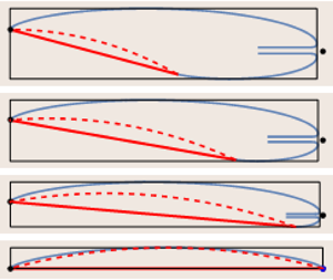
Consider figure 5, where the shapes of the cavities for four small angles of attack $\alpha =2^\circ$, $1^\circ$, $0.5^\circ$ and $0.05^\circ$ at the cavity number $\sigma =0.6$ are shown. As one can see, at $\alpha \le 2^\circ$, the cavity closure region becomes close to the trailing edge $B$. With decrease of angles of attack, the width $\delta$ of the re-entrant almost vanishes, and the cavity tends to be symmetric with respect to the axis that is perpendicular to the plate surface and goes through the middle of the plate. This symmetry explains why $r/l\to 1/2$ as $\alpha \to 0$. Figures 5(e–h) demonstrate the cavity closure regions including the cavity shapes and the shapes of dividing streamlines. A surprising fact is that at $\alpha =0.05^\circ$, the inner stagnation point migrates downwards and locates lower than the $x$-axis.

Figure 5. The shapes of the plate and cavities at $\beta ={\rm \pi}$, $\sigma =0.6$, and different small angles of attack $\alpha$. Panels (e–h) show the corresponding cavity closure regions.

In figure 6, the distributions of the pressure coefficient

(5.1)\begin{equation} C_p=\frac{p-p_0}{\rho v_\infty^2/2} \end{equation}

are presented for the same cavity number, $\sigma =0.6$, as in figure 5, at angles of attack $\alpha =8^\circ$, $5^\circ$, $2^\circ$, $1^\circ$, $0.5^\circ$, $0.05^\circ$ (curves 1–6). All these $\alpha$ are from the ‘abnormal’ range of angles of attack $\alpha \in (0,\alpha _1]$. Curves 3–6 in figure 6 correspond to figures 5(e–h). Figures 5 and 6 explain the increase of $C_N$ and $C_L$ with decrease of $\alpha$. Indeed, in the ‘abnormal’ range, the inner stagnation point $C$ in the cavity closure region locates very closely to the trailing edge $B$. Since at the stagnation point $C$ the pressure achieves its maximum, this maximum influences the pressure distribution near the trailing edge, and the normal force increases together with the lift as the stagnation point approaches the trailing edge.

Figure 6. The distribution of the pressure coefficient $C_p$, determined by (5.1), at $\sigma =0.6$ and $\alpha =8^\circ$, $5^\circ$, $2^\circ$, $1^\circ$, $0.5^\circ$, $0,05^\circ$ (curves 1–6). The $x$-axis is directed along the plate.

Let us continue to diminish the angles of attack (see figure 7). In the scale of the length $l$, the full cavity shapes for $\alpha <0.05^\circ$, are almost indistinguishable from that in figure 5 at $\alpha =0.05^\circ$. So for $\alpha <0.05^\circ$, we have plotted in figure 7 only the cavity closure regions. The arrows indicates the direction of the flow, abbreviations RJ and DSL mean ‘re-entrant jet’ and ‘dividing streamline’, respectively.

Figure 7. The cavity closure regions at $\beta ={\rm \pi}$, $\sigma =0.6$, and very small angles of attack $\alpha$. The arrows indicate the directions of the velocity vectors.

At $\alpha =0.03^\circ$, the inner stagnation point is very close to the lower side of the plate. At $\alpha =\alpha _{crit}=0.0293412^\circ$, the stagnation point locates directly on the lower plate surface (see figure 7b). Mathematically, this means that the accessory parameter is $c=0$. The angles of attack at which $c=0$ we shall call critical and denote by $\alpha _{crit}$. At $\beta ={\rm \pi}$, the angle $\alpha _{crit}$ depends only on the cavity number $\sigma$. In table 3, we present the angles $\alpha _{crit}$ for several values of $\sigma$, and as one can see, these angles turn out to be very small.

Table 3. Critical angles of attack versus the cavity number $\sigma$.

At $\alpha <\alpha _{crit}$, the parameter $c$ becomes imaginary, which gives rise to two stagnation points lying directly on the lower side of the plate (see figure 7c, $\alpha =0.027^\circ$). In the parametric $t$-plane, the images of these points are $u_{01}=c+\mathrm {i} d$ and $u_{02}=-c+\mathrm {i} d$, and because $c$ is imaginary, both images lie on the imaginary axis $\eta$. Nevertheless, all equations that have been deduced earlier remain correct, although one should take into account that in (2.1) and (2.3), $u_0=c+\mathrm {i} d$, but $\overline {u_0}=c-\mathrm {i} d$ (as before), in spite of the fact that $c$ is imaginary.

For all three cavity closure regions shown in figure 7, the width $\delta$ of the re-entrant jet is less than $10^{-4}l$. It is worthwhile noting also that at $\alpha <\alpha _{crit}$ (figure 7c), a small segment appears between two stagnation points on the plate surface, where the direction of the flow is opposite to the $x$-axis. As $\alpha \to 0$, the length of the segment increases, the width of the re-entrant jet $\delta$ tends to $0$, the right stagnation point tends to the trailing edge $B$, and the left one shifts to the left, tending to a quite definite location. The limit is the flow that will be investigated in the next section.

6. The limiting flow configurations as $\alpha \to 0$

A sketch of the limiting flow at $\alpha =0$ is shown in figure 8(a). The flow is symmetric with respect to the axis that is directed vertically upwards and goes through the middle of the plate. The flow has a symmetric cavity located above the plate, and two stagnation points $K$ and $C$, the re-entrant jet being absent ($\delta =0$). The incident velocity $v_\infty$ and the cavity number $\sigma$, defined by (1.2), are assumed to be given. As the parametric domain, we choose the upper semicircle of the $t$-plane shown in figure 8(b). By virtue of symmetry, the images of the stagnation points $K$ and $C$ are $m$ and $-m$, respectively, and the image of the point $D$ at infinity is $\mathrm {i} n$, i.e. it lies on the imaginary axis. Making use of Chaplygin's method of singular points (see Gurevich Reference Gurevich1965), we find

(6.1a,b)\begin{equation} \frac{\mathrm{d} w}{\mathrm{d} t}=l_0 v_0\,f(t),\quad f(t)=\frac{(1-t^2) (t^2-m^2)(1-m^2 t^2)}{(t^2+n^2)^2(1+n^2 t^2)^2}, \end{equation}

where $l_0$ is an unknown positive constant, which has the dimension of length.

Figure 8. (a) Sketch of the limiting flow configuration at $\alpha =0$. (b) Parametric $t$-plane together with streamlines.

Further, by the same method we determine

(6.2a,b)\begin{gather} \frac{\mathrm{d} w}{v_0\,\mathrm{d} z}=F(t), \quad F(t)=\frac{m^2-t^2}{1-m^2 t^2}, \end{gather}

(6.3a,b)\begin{gather} \frac{\mathrm{d} z}{\mathrm{d} t}=l_0\,\frac{f(t)}{F(t)}=G(t), \quad G(t)=\frac{(t^2-1)(1-m^2 t^2)^2}{(t^2+n^2)^2(1+n^2 t^2)^2}. \end{gather}

So the problem has three unknown accessory parameters: $l_0$, $m$ and $n$. To determine these parameters, we deduce the three equations

(6.4a–c)\begin{equation} 1-3 n^2-3 m^2 n^2 +m^2 n^4 =0,\quad \frac{m^2+n^2}{1+m^2 n^2}=R,\quad l=l_0\,J(m,n), \end{equation}

where $R$ is defined by (2.9), and $J=\int _{-1}^1 G(\xi )\,\mathrm {d}\xi$. Equation (6.4a) follows from the closure condition $\mathop {{\rm{res}}}\limits_{t=\mathrm {i} n}{G(t)}=0$, (6.4b) is a consequence of the relation $F(\mathrm {i} n)=R$, analogous to (2.8), and (6.4c) connects the length $l$ of the plate with the parameter $l_0$.

The solution to the system of (6.4a) and (6.4b) is

(6.5a–c)\begin{equation} m=\sqrt{\frac{(2-U)(U+1)}{(2+U)(U-1)}}, \quad n=\sqrt{\frac{U-1}{U+1}}, \quad U=\sqrt{1+\sqrt{1+\sigma}}. \end{equation}

Since we have $m\ge 0$, we conclude from (6.5a) that $U\le 2$ and therefore $0<\sigma \le 8$.

For the parameter $J$ and the conformal mapping $z(t)$, after a little algebra, we obtain

(6.6)\begin{equation} J=\frac{4 \mu}{n^2+1}\left(R+\frac{1}{R}\right)-\frac{4\gamma}{\rm \pi}\tan^{{-}1}n, \end{equation}

where

(6.7)\begin{gather} \mu=\lim_{t\to \mathrm{i} n}f(t)(t-\mathrm{i} n)^2=\frac{(1+U)^3}{2 U (U^2+U-2)^2}, \end{gather}

(6.8)\begin{gather} \gamma={-}2 {\rm \pi}\mathrm{i} \mathop {{\rm{res}}}\limits_{t=\mathrm{i} n}{f(t)}={-}\frac{\rm \pi}{2}\, \frac{(1+U)^{7/2}(U^2-2)}{(U-1)^{5/2}(U+2)^2}, \end{gather}

(6.9a,b)\begin{gather} z(t)=\frac{1}{J}\,\zeta(t)-\frac{1}{2},\quad \zeta(t)={-}\frac{2 \mu t}{R (t^2+n^2)}-\frac{2 \mu R t}{1+n^2 t^2}+\frac{4\gamma R}{\rm \pi}\tan^{{-}1}(nt). \end{gather}

The lift force $N$ for the limiting flows over the plate is computed by the Kutta–Joukowski theorem: $N=-\rho v_\infty \varGamma$, where the circulation satisfies $\varGamma\!=l_0 v_0 \gamma$. Therefore,

(6.10)\begin{equation} C_{N\,lim}=C_{L\,lim}={-}2 \gamma\sqrt{1+\sigma}/J. \end{equation}

Due to d'Alembert's paradox, $C_D=0$ for the limiting flows.

In figure 9, the shapes of the cavities for the limiting flows are presented. The number in front of the leading edges on the ordinate axis indicates the cavity number $\sigma$ at which the limiting configuration has been constructed. The configurations are shifted by 0.1 with respect to each other in the vertical direction. An interesting fact is that in each of the limiting cavities, it is possible to inscribe a very simple geometric figure, namely, a circular segment of the same width $h$ as that of the cavity. In figure 9, these segments are plotted by the dashed lines.

Figure 9. The shapes of the cavity bubbles for the limiting flows (solid lines). The numbers in front of the leading edges on the ordinate axis correspond to the cavity number $\sigma$. The dashed lines show the circular segments inscribed in the cavities.

7. Comparison with experimental data

Dawson & Bate (Reference Dawson and Bate1962) measured the pressure distribution on the lower side of the cavitating wedge with angle $6^{\circ }$ at the vertex. The wedge was located in a free-surface water tunnel, and one of the investigated depths (maximal) was 2.16 model chords. Assuming that such a depth is enough to neglect the influence of the free surface, we compare the results of our computations with the experimental data by Dawson & Bate (Reference Dawson and Bate1962). The comparison is shown in figure 10, and as one can see, the agreement looks quite satisfactory.

Figure 10. Distribution of the pressure coefficient $C_p$, determined by (5.1), at $\alpha =8^\circ,10^\circ,12^\circ,14^\circ$. The corresponding cavity numbers are $\sigma =0.115, 0.111, 0.127,0.12$. The $x$-axis is directed along the plate. The disks, circles, triangles and filled triangles are the experimental results by Dawson & Bate (Reference Dawson and Bate1962).

Wade (Reference Wade1964) and Wade & Acosta (Reference Wade and Acosta1966) reported the results of the experiments for cavitating flows over a circular segment of width $6.9\,\%$. The report by Wade (Reference Wade1964) contains tables with the data for $C_L$, $C_D$ and the coefficients of the moment measured with respect to the middle of the plate. The data are presented for four angles of attack: $\alpha =4^\circ, 6^\circ, 8^\circ, 10^\circ$. It is evident that

(7.1a,b)\begin{gather} C_N=C_L\cos\alpha+C_D \sin\alpha, \quad C_M=C_{MW}-\tfrac{1}{2}(C_L \cos\alpha+C_D \sin\alpha), \end{gather}

(7.2)\begin{gather} C_\tau=C_D \cos\alpha-C_L \sin\alpha, \end{gather}

where $C_\tau$ is the coefficient of the force tangential to the plate (in the ideal fluid, $C_\tau =0$), and $C_{MW}$ is the moment coefficient from Wade's tables taken with opposite sign, due to the mirror location (with respect to ours) of the hydrofoil and the incident flow in the experiments by Wade (Reference Wade1964). Thus, using (7.1) and (7.2), we have recalculated Wade's data for $C_N$, $C_M$ and $C_\tau$.

The results of the comparison are shown in figure 11. As one can see, the agreement again looks satisfactory even for cases of short cavities when $L_c/L<1.2$, i.e. when Wade's instability criterion of the cavity is fulfilled. As can be expected, the experimental values of $C_\tau$ turn out to be small. When $L_c/L<1.2$, these values become negative, which can be explained by the influence of the re-entrant jet.

Figure 11. Solid lines are the graphs of $C_N(\sigma )$ (positive values) and $C_M(\sigma )$ (negative values). Disks are the results of Wade (Reference Wade1964) recalculated by formulae (7.1a,b). The disks close to the $\sigma$-axes are the results for the coefficients $C_\tau$ of the tangential force. The arrows together with the figures above them indicate the cavity numbers $\sigma$ at which the corresponding $L_c/l$ are attained. The dashed lines are obtained from formulae of the linear theory (Geurst Reference Geurst1960).

In figure 11, the dashed lines are plotted with the help of simple analytical formulae of the linear theory presented in the paper by Geurst (Reference Geurst1960). As one can see, this theory gives results that are very close to ours, which is not surprising because in the experiments by Wade & Acosta (Reference Wade and Acosta1966), the angles of attack are small (from $4^\circ$ to $10^\circ$).

8. Concluding remarks

In the paper, we have demonstrated that the uncertainty of the potential re-entrant jet cavity model can be fixed by minimizing the kinetic energy of the jet. Our calculations of cavity flows over oblique flat plates, based on the energy criterion, confirm the conjecture made by Terentiev et al. (Reference Terentiev, Kirschner and Uhlman2011) that the direction of the re-entrant jet should be opposite to the incident flow. Since for the flat plate the conclusion turns out to be correct for any angle of attack $\alpha$ and any cavity number $\sigma \le 1$, we assume that the energy principle will lead to the same result for a curved plate of any shape. The approximate formula (3.2), whose deduction is independent of the plate shape, confirms this conclusion too.

An oblique flat plate is the simplest lifting shape, and the cavity flow over such a shape can be considered as a test problem for any cavity model. Another question studied in the paper is that of the limiting passage when the cavity number $\sigma >0$ is fixed and the angle of attack $\alpha$ tends to zero. A natural limit of uniform flow here is impossible because the cavity number remains finite. In our opinion, such a limit gives a general characteristic of any cavity model. Let us compare the limit for the re-entrant jet model with that given by the linear theory (see Geurst Reference Geurst1960) for which

(8.1a,b)\begin{equation} C_L=C_N=\frac{{\rm \pi} \left(4 \alpha ^2+\sigma ^2\right)}{2 \left(\sqrt{4 \alpha ^2+\sigma ^2}+2 \alpha \right)},\quad C_L(\alpha\to 0)=C_{L\,lim}= \frac{\rm \pi}{2}\sigma. \end{equation}

In the linear theory, a slight singularity at the end of the cavity occurs in a natural way from the solution of the corresponding boundary-value problem. So in the linear theory, we do not have any artificial bodies in the cavity closure region. For the re-entrant jet model, such bodies are also absent. Making use of formulae (6.5)–(6.8) and (6.10), for the limiting re-entrant jet flow, we get the expression

(8.2)\begin{equation} C_{L\,lim}=\frac{\rm \pi}{2}\sigma +O(\sigma^2). \end{equation}

Comparing (8.1b) and (8.2), one can see that at $\alpha =0$ and $\sigma \to 0$, the linear theory and the re-entrant jet model give the same results.

The limiting passage $\alpha \to 0$ is characterized by the following features.

1. (i) At small $\alpha \in (0,\alpha _1)$, the lift force $L$ displays an abnormal behaviour: the lift coefficient $C_L$ increases as $\alpha$ decreases (see figure 4 and table 2).

2. (ii) As $\alpha \to 0$, the width of the re-entrant jet $\delta$ and the drag coefficient $C_D$ tend to zero, whereas the lift coefficient $C_L$ tends to a finite and rather significant value.

3. (iii) The stagnation point $C$ migrates downwards and at a certain $\alpha =\alpha _{crit}$ locates on the lower side of the plate $AB$ very closely to the trailing edge $B$ (see figures 5 and 7, and table 3).

4. (iv) An almost symmetric bubble forms above the plate, which becomes fully symmetric at $\alpha =0$ (see figures 5 and 9).

If the stable bubble from point (iv) or something similar to it were realizable, then the large lift at small angle of attack $\alpha$ would be possible too. So the question is how such a bubble could be created. Our computations show that the bubble forms when the cavity length is very short ($L_c/l<4/3$). According to Brennen (Reference Brennen1995), this is the transition regime from steady cavity flow to cloud cavitation. Here some methods of control of the cloud cavitation can be helpful (see Kawanami et al. Reference Kawanami, Kato, Yamaguchi and Tagaya1997; Zhang, Chen & Shao Reference Zhang, Chen and Shao2018).

In the literature, we have not found comparison of the results obtained by the re-entrant jet cavity model with experimental data. In § 7 of our paper, we make such a comparison and reveal good agreement.

In the supplementary materials to the paper, we store the file Algorithm.pdf, which contains the description of the algorithm for finding the accessory parameters and the deduction of pure analytical, integral-free formulae for all hydrodynamic properties. Also in these materials there are files ReentrantJet.m and ReentrantJet_Usage.nb. In the Wolfram Mathematica package ReentrantJet.m, the algorithm and formulae from Algorithm.pdf are programmed, and the notebook ReentrantJet_Usage.nb explains the usage of the package ReentrantJet.m.