


1. Introduction
In this paper we extend the asymptotic receptivity theory to the boundary-layer flow in presence of a thin liquid film covering the body surface. The receptivity theory describes the early stage of laminar–turbulent transition of flows where the instability modes in the boundary layer are formed due to external perturbations. For the laminar–turbulent transition, the most ‘dangerous’ are the instability modes (like Tollmien–Schlichting waves) that are generated near the lower branch of the instability curve. In this case they have enough space to grow downstream to cause the nonlinear effects characteristic of the turbulent flow. In flight conditions aircraft travel with high speed, which allows us to assume the Reynolds number is large in our analyses. Neiland (Reference Neiland1969) and Stewartson & Williams (Reference Stewartson and Williams1969) were the first to theoretically describe separation of flows with sufficiently large value of the Reynolds number. They formulated the boundary-layer instability near the lower branch by so-called triple-deck theory. Almost at the same time, Stewartson (Reference Stewartson1969) and Messiter (Reference Messiter1970) suggested that to describe the behaviour of incompressible fluid flows near the trailing edge of a flat plat one can use the triple-deck theory. Thenceforth, it became evident that this theory is effective in describing the boundary layer and its interaction with free-stream flow. Therefore triple-deck theory has been receiving a great deal of attention ever since and it has been extended to wide range of problems in fluid dynamics such as the monograph by Sychev et al. (Reference Sychev, Ruban, Sychev and Korolev1998) and, in a more recent study, Ruban (Reference Ruban2018) focuses on the boundary-layer separation.
Further progress was made by Schneider (Reference Schneider1974) where he used the same viscous–inviscid structure to describe unsteady flows. He found that the layer of flow located near the wall is the most sensitive to unsteady perturbations where the fluid velocity is relatively small. He demonstrated that the flow in this layer becomes unsteady when the characteristic time,  $t$, of the variation of the perturbations is of order
  $t \sim Re^{-1/4}$ quantity; here,
  $Re$ denotes the Reynolds number. Other important theoretical works using this theory were conducted by Lin (Reference Lin1946) and Smith (Reference Smith1979a,Reference Smithb). Lin analysed the asymptotic behaviour of the lower and upper branches of the neural stability curve in incompressible boundary layers. While assuming Reynolds number is larger,
  $Re \rightarrow \infty$, he first solved the Orr–Sommerfeld equation. Then, working on the lower branch, he found that the description of the flow requires a three-layered structure. As a result of this analysis Lin found the frequency of the oscillations and the wavenumber appear to be
  $\omega = O (Re^{1/4})$ and
  $k = O (Re^{3/8})$, respectively. Then Smith (Reference Smith1979a,Reference Smithb) strengthened the application of triple-deck theory to subsonic flows to describe the Tollmien–Schlichting waves at and near the lower branch of the neutral stability curve. We develop a modified triple-deck theory to conduct receptivity analysis for a multi-fluid flow over a flat plate with a small roughness on the surface. Note that it was Terent'ev (Reference Terent'ev1981) who initially used this theory to study boundary-layer receptivity and produced a simplified theoretical model for an earlier experimental work by Schubauer & Skramsted (Reference Schubauer and Skramsted1948) where the instability waves in the boundary layer were generated by a vibrating ribbon installed a small distance above the plate surface. For an effective generation of the instability waves, Terent'ev (Reference Terent'ev1981) considered an unsteady flow over a flat plate where a short section of plate is oscillating with respect to time. He let the length of the vibrating section coincide with the length scale in the classical triple-deck theory and found that the frequency of the vibrating wall must be
  $\omega \sim O (Re^{1/4})$ for the triple-deck to hold. Terent'ev (Reference Terent'ev1981) derived the amplitude of the instability waves (Tollmien–Schlichting waves) and showed that the perturbations produced by the vibrating wall become rapidly damped upstream. However, downstream, the damping weakens as the frequency approaches the critical value of frequency predicted by the classical instability theory. We know that there are no vibrating ribbons on the wing surface, in real flights, however, there are various disturbances in the oncoming flow around the aircraft which lead to formation of Tollmien–Schlichting waves. Experimental observations show (see, for e.g. Kachanov, Kozlov & Levchenko Reference Kachanov, Kozlov and Levchenko1982; Saric, Hoos & Radeztsky Reference Saric, Hoos and Radeztsky1991) that the boundary layers are susceptible to some but not to all external perturbations. Acoustic waves are one class of disturbance that boundary layers are susceptible to and they are always found in the flow field around an aircraft and easily penetrate the boundary layer. For theoretical analysis of such disturbance we need to satisfy two resonance conditions, the so-called double-resonance principle, compared with simple mechanical systems. Where resonance forces are simply formed as the frequency
  $\omega$ of the external forcing coincides with the natural frequency of the system. For fluid systems we need to consider an additional condition with respect to the wavenumber of the external perturbations. These perturbations must be in tune with the natural internal oscillations of the boundary layer. To satisfy the resonance conditions in the ‘vibrating ribbon’ problem, Terent'ev (Reference Terent'ev1981) suggested that the frequency and the length of the vibrating part of the wall should be chosen according to the double-resonance principle. Extending the earlier work of Kachanov et al. (Reference Kachanov, Kozlov and Levchenko1982), which is based on the resonance conditions in fluids, Ruban (Reference Ruban1984) and Goldstein (Reference Goldstein1985) showed that the acoustic wave has to come into interaction with wall roughness. To satisfy the resonance conditions, with respect to the wavenumber, that lead to the generation of Tollmien–Schlichting waves in the boundary layer they assumed (i) the frequency of the external acoustic wave and (ii) the length of the roughness must be
  $O (Re^{1/4})$ and
  $O (Re^{-3/8})$, respectively. With these scalings the triple-deck theory is valid and describes the flow around the roughness which ultimately enables us to determine the initial amplitude of the Tollmien–Schlichting waves in the boundary layer. They also demonstrated that satisfying only the first condition is insufficient to generate the Tollmien–Schlichting waves because the speed of propagation of acoustic waves is finite and the wavelength appears to be
  $\ell \sim Re^{-1/4}$, which is much longer than the wavelength of the Tollmien–Schlichting wave.
Later, the triple-deck theory was extended to other receptivity mechanisms. These include the generation of Görtler vortices by wall roughness (see Denier, Hall & Seddougui Reference Denier, Hall and Seddougui1991) and the generation of the Tollmien–Schlichting waves by the interaction between free-stream turbulence and a small wall roughness in the boundary layer (see Duck, Ruban & Zhikharev Reference Duck, Ruban and Zhikharev1996). A possibility of efficient receptivity without a wall roughness was demonstrated by Wu (Reference Wu1999), who showed how the double-resonance conditions may be satisfied when an acoustic wave interacts with the free-stream turbulence. He also extended the theory of Ruban (Reference Ruban1984) and Goldstein (Reference Goldstein1985) to the case of distributed wall roughness; see Wu (Reference Wu2001). The asymptotic receptivity theory is easily adjusted to different flow speed regimes. In particular, Ruban, Bernots & Kravtsova (Reference Ruban, Bernots and Kravtsova2016) studied the receptivity of the boundary layer to acoustic waves in transonic flows and Dong, Liu & Wu (Reference Dong, Liu and Wu2020) performed the corresponding analysis for supersonic flows. Recently, using the triple-deck theory, Brennan, Gajjar & Hewitt (Reference Brennan, Gajjar and Hewitt2021) studied a possibility of controlling the receptivity of the boundary layer. There are also number of stability analyses of flows past a thin liquid film such as Coward & Hall (Reference Coward and Hall1996), Timoshin (Reference Timoshin1997) and Tsao, Rothmayer & Ruban (Reference Tsao, Rothmayer and Ruban1997). A more recent study using the triple-deck model was performed by Cimpeanu et al. (Reference Cimpeanu, Papageorgiou, Kravtsova and Ruban2015) with the purpose of investigating the influence of the film on the separation of the boundary layer.
In this paper we conduct the receptivity analysis of high-speed flows over a thin liquid film. Given that there is a lot of roughness on a wing's surface, we assume there is a small roughness in the boundary layer. The analysis of the generation of the interfacial waves is performed under the assumption that the ratio of the viscosity coefficients in the air and in the film,  $\sigma _{\mu }$, is small. Guided by the double-resonance principle, we choose the frequency of the acoustic wave to be an order
  $O (Re^{1/4} \sigma _{\mu })$ quantity. Corresponding to this, the thickness of the Stokes layer, forming in the airflow just above the film, is
  $O (\sigma _{\mu }^{-1/2} Re^{-5/8})$. Meanwhile, the thickness of the film is taken to be an
  $O (Re^{-5/8})$ quantity. To satisfy the resonance conditions, we further assume that length of the roughness is an
  $O (Re^{-3/8})$ quantity. Ultimately the Tollmien–Schlichting waves are formed as the result of interaction between the Stokes layer and the perturbations produced by the wall roughness. Amplitude of these waves are found in an explicit analytic form.
2. Problem formulation
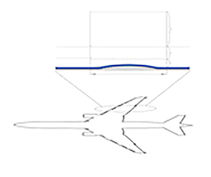
Let us consider a perfect gas flow past a flat plate coated by a liquid film. For simplicity we shall assume that the plate is aligned with the velocity vector in the oncoming flow; see figure 1. We shall further assume that the flow is exposed to weak acoustic waves. Our task will be to study the interaction of these waves with a small roughness on the plate surface at distance  $L$ from the leading edge. In what follows we shall assume that the flow is two-dimensional. To study the flow we use the Cartesian coordinates
  $(\hat {x}, \hat {y})$, with
  $\hat {x}$ measured along the flat plate surface from its leading edge
  $O$, and
  $\hat {y}$ in the perpendicular direction. The velocity components in these coordinates are denoted by
  $(\hat {u} , \hat {v})$. As usual, we denote the time by
  $\hat {t}$, the gas density by
  $\hat {\rho }$, pressure by
  $\hat {p}$, enthalpy by
  $\hat {h}$ and dynamic viscosity coefficient by
  $\hat {\mu }$. The ‘hat’ is used here for dimensional variables and ‘prime’ for the fluid-dynamic functions in the liquid film. The non-dimensional variables in the airflow are introduced as follows:
 \begin{equation} \left.\begin{gathered} \hat{t} = \frac{L}{V_{\infty }} t ,\quad \hat{x} = L x ,\quad \hat{y} = L y ,\\ \hat{u} = V_{\infty } u , \quad \hat{v} = V_{\infty } v, \quad \hat{\rho } = \rho _{\infty } \rho ,\\ \hat{p} = p_{\infty } + \rho _{\infty } V_{\infty }^2 p , \quad \hat{h} = V_{\infty }^2 h, \quad \hat{\mu } = \mu _{\infty } \mu , \end{gathered} \right\} \end{equation}
with  $V_{\infty }$,
  $p_{\infty }$,
  $\rho _{\infty }$ and
  $\mu _{\infty }$ being the dimensional free-stream velocity, pressure, density and viscosity, respectively. In non-dimensional variables, the Navier–Stokes equations are written as
 \begin{gather} \rho \left( \frac{\partial u}{\partial t} + u \frac{\partial u}{\partial x} + v \frac{\partial u}{\partial y} \right) ={-} \frac{\partial p}{\partial x} + \frac{1}{Re} \left\{ \frac{\partial }{\partial x} \left[ \mu \left( \frac{4}{3} \frac{\partial u} {\partial x} - \frac{2}{3} \frac{\partial v}{\partial y} \right) \right]\right. \nonumber\\ \hspace{8pc}\left. + \frac{\partial }{\partial y} \left[ \mu \left( \frac{\partial u}{\partial y} + \frac{\partial v}{\partial x} \right) \right] \right\} , \end{gather}
 \begin{gather} \rho \left( \frac{\partial v}{\partial t} + u \frac{\partial v}{\partial x} + v \frac{\partial v}{\partial y} \right) ={-} \frac{\partial p}{\partial y} + \frac{1}{Re} \left\{ \frac{\partial }{\partial y} \left[ \mu \left( \frac{4}{3} \frac{\partial v} {\partial y} - \frac{2}{3} \frac{\partial u}{\partial x} \right) \right] \right.\nonumber\\ \hspace{8pc} \left. + \frac{\partial }{\partial x} \left[ \mu \left( \frac{\partial u}{\partial y} + \frac{\partial v}{\partial x} \right) \right] \right\} , \end{gather}
 \begin{gather} \hspace{-23pc} \rho \left( \frac{\partial h}{\partial t} + u \frac{\partial h}{\partial x} + v \frac{\partial h}{\partial y} \right) \nonumber\\ \hspace{-6pc} = \frac{\partial p}{\partial t} + u \frac{\partial p}{\partial x} + v \frac{\partial p}{\partial y} + \frac{1}{Re} \left\{ \frac{1}{Pr} \left[ \frac{\partial }{\partial x} \left( \mu \frac{\partial h}{\partial x} \right) + \frac{\partial }{\partial y} \left(\mu \frac{\partial h}{\partial y} \right) \right] \right.\nonumber\\ \qquad \left.+ \mu \left( \frac{4}{3} \frac{\partial u}{\partial x} - \frac{2}{3} \frac{\partial v}{\partial y} \right) \frac{\partial u}{\partial x} + \mu \left( \frac{4}{3} \frac{\partial v}{\partial y} - \frac{2}{3} \frac{\partial u}{\partial x} \right) \frac{\partial v}{\partial y} + \mu \left( \frac{\partial u}{\partial y} + \frac{\partial v}{\partial x} \right) ^2 \right\} , \end{gather}
 \begin{gather} \frac{\partial \rho }{\partial t} + \frac{\partial \rho u}{\partial x} + \frac{\partial \rho v}{\partial y} = 0 , \end{gather}
 \begin{gather} h = \frac{1}{(\gamma - 1) M_{\infty }^2} \frac{1}{\rho } + \frac{\gamma } {\gamma -1} \frac{p}{\rho } . \end{gather}
Here,  $Pr$ is the Prandtl number and
  $\gamma$ is the specific heat ratio; for air
  $Pr \approx 0.713$,
  $\gamma = 7/5$. The Reynolds number
  $Re$ is calculated as
 \begin{equation} Re = \frac{\rho _{\infty } V_{\infty } L}{\mu _{\infty }} . \end{equation}
In this study, we shall assume that  $Re$ is large, while the free-stream Mach number,
 \begin{equation} M_{\infty } = \frac{V_{\infty }}{a_{\infty }} , \end{equation}
remains finite. In fact, we shall restrict our attention to subsonic flows where  $M_{\infty } < 1$. Remember that the speed of sound
  $a_{\infty }$ in (2.4) is calculated as
 \begin{equation} a_{\infty } = \sqrt{\gamma \frac{p_{\infty }}{\rho _{\infty }}} . \end{equation}
When performing the flow analysis we shall assume (Coward & Hall Reference Coward and Hall1996) that the viscosity and density ratios
 \begin{equation} \sigma_{\mu}=\frac{\mu _{\infty }}{\hat{\mu }^{\prime }}, \quad \sigma_{\rho}= \frac{\rho _{\infty }}{\hat{\rho}^{\prime }} \end{equation}
are small.

Figure 1. Flow layout, the blue layer represents the liquid film.
3. The flow before the roughness
We start with region 1 that lies outside the boundary layer, see figure 1.
3.1. Inviscid airflow (region 1)
In this region we have a uniform flow which is perturbed by an acoustic wave. For simplicity, we shall assume that the acoustic wave propagates along the main flow with the front of the wave being perpendicular to the plate surface. Consequently, we represent the fluid-dynamic functions in region 1 in the form of the asymptotic expansions
 \begin{equation} \left.\begin{gathered} u = 1 + \sigma _{\mu }^{{-}1/2} Re^{{-}1/8} \chi u_1 (t_{{\ast} } , x_1) + \cdots , \\ p = \sigma _{\mu }^{{-}1/2} Re^{{-}1/8} \chi p_1 (t_{{\ast} } , x_1) + \cdots , \\ h = \frac{1}{(\gamma - 1) M_{\infty }^2} + \sigma _{\mu }^{{-}1/2} Re^{{-}1/8} \chi h_1 (t_{{\ast} } , x_1) + \cdots , \\ \rho = 1 + \sigma _{\mu }^{{-}1/2} Re^{{-}1/8} \chi \rho _1 (t_{{\ast} } , x_1) + \cdots , \end{gathered}\right\} \end{equation}
with the independent variables  $t_{\ast }$,
  $x_1$ defined by
 \begin{equation} t = \sigma _{\mu }^{{-}1} Re^{{-}1/4} t_{{\ast} } , \quad x = 1 + \sigma _{\mu }^{{-}1} Re^{{-}1/4} x_1 . \end{equation}
 Note that the viscosity coefficient is zero in the inviscid region. In (3.1), the amplitude of acoustic wave  $\sigma _{\mu }^{-1/2} Re^{-1/8} \chi$ is chosen such that for
  $\chi = O (1)$ the perturbations appear to be nonlinear in the Stokes layer (region 3 in figure 1). We shall see that the frequency of the interfacial instability waves is an order
  $O (\sigma _{\mu } Re^{1/4})$ quantity, which explains the choice of the scaling factor in the equation for
  $t$ in (3.2a,b). Since the speed of propagation of acoustic waves is finite, the wavelength appears to be
  $O (\sigma _{\mu }^{-1} Re^{-1/4})$ which is used to scale
  $x$ in (3.2a,b).
Substituting (3.1) and (3.2a,b) into the Navier–Stokes equations (2.2) and assuming that  $\sigma _{\mu }^{-1/2}Re^{-1/8} \chi$ is small, results in the following set of linearised Euler equations:
 \begin{equation} \left.\begin{gathered} \frac{\partial u_1}{\partial t_{{\ast} }} + \frac{\partial u_1}{\partial x_1} ={-} \frac{\partial p_1}{\partial x_1} , \\ \frac{\partial h_1}{\partial t_{{\ast} }} + \frac{\partial h_1}{\partial x_1} = \frac{\partial p_1}{\partial t_{{\ast} }} + \frac{\partial p_1}{\partial x_1} ,\\ \frac{\partial \rho _1}{\partial t_{{\ast} }} + \frac{\partial u_1}{\partial x_1} + \frac{\partial \rho _1}{\partial x_1} = 0 , \\ h_1 = \frac{\gamma }{\gamma - 1} p_1 - \frac{1}{(\gamma - 1) M_{\infty }^2} \rho _1 . \end{gathered}\right\} \end{equation}
These may be reduced to a single equation for the pressure
 \begin{equation} M_{\infty }^2 \frac{\partial ^2 p_1}{\partial t_{{\ast} }^2} + (M_{\infty }^2 - 1) M_{\infty }^2 \frac{\partial ^2 p_1}{\partial x_1^2} + 2 M_{\infty }^2 \frac{\partial ^2 p_1}{\partial t_{{\ast} } \partial x_1} = 0 . \end{equation}
By definition (3.3), the enthalpy  $h_1$ depends on
  $M_{\infty }$, hence the factor of
  $M_{\infty }$ appears in the pressure governing equation (3.4).
The solution to (3.4) representing a monochromatic acoustic wave is written as
 \begin{equation} p_1 = p_a (t_{{\ast} } , x_1) = \alpha \sin (\omega t_{{\ast} } + k_a x_1) , \end{equation}
with the other fluid-dynamic functions being
 \begin{equation} u_1 = M_{\infty } p_a , \quad \rho _1 = M_{\infty }^2 p_a , \quad h_1 = p_a . \end{equation}
Here,  $k_a$ in the wavenumber of the acoustic wave given by
 \begin{equation} k_a ={-} \frac{M_{\infty }}{M_{\infty } + 1} \omega . \end{equation}
We shall show how this slow acoustic wave leads to the formation of a slow motion air layer, the so-called Stoke layer, in the boundary layer.
3.2. Main part of the boundary layer (region 2)
Now we shall see how the acoustic wave penetrates the boundary layer. When there is no acoustic wave, the flow inside the boundary layer is given by the compressible version of the Blasius solution
 \begin{equation} \left.\begin{gathered} u = U_0 (x , y_2) + \cdots , \quad v = Re^{{-}1/2} V_0 (x , y_2) + \cdots , \\ p = Re^{{-}1/2} P_0 (x , y_2) + \cdots , \quad \rho = \rho_0 (x , y_2) + \cdots , \\ h = h_0 (x , y_2) + \cdots , \quad \mu = \mu _0 (x , y_2) + \cdots , \end{gathered}\right\} \end{equation}
where
 \begin{equation} y_2 = Re^{1/2} y . \end{equation}
The behaviour of the leading-order terms in (3.8) were studied by various authors (see, for e.g. Ruban Reference Ruban2018). It is known that by substituting (3.8) into the Navier–Stokes equations (2.2) a boundary-value problem is derived which admits a self-similar solution for certain conditions. In the presence of the acoustic wave, asymptotic expansions (3.8) become
 \begin{equation} \left.\begin{gathered} u = U_0 (x , y_2) + \sigma _{\mu }^{{-}1/2} Re^{{-}1/8} \chi u_2 (t_{{\ast} } , x_1 , y_2) +\cdots ,\\ v = \sigma ^{1/2} Re^{{-}3/8} \chi v_2 (t_{{\ast} } , x_1 , y_2) + \cdots , \\ p = \sigma _{\mu }^{{-}1/2} Re^{{-}1/8} \chi p_2 (t_{{\ast} } , x_1 , y_2) + \cdots , \\ \rho = \rho_0 (x , y_2) + \sigma _{\mu }^{{-}1/2} Re^{{-}1/8} \chi \rho _2 (t_{{\ast} } , x_1 , y_2) + \cdots , \\ h = h_0 (x , y_2) + \sigma _{\mu }^{{-}1/2} Re^{{-}1/8} h_2 \chi (t_{{\ast} } , x_1 , y_2) + \cdots , \\ \mu = \mu _0 (x , y_2) + \sigma _{\mu }^{{-}1/2} Re^{{-}1/8} \chi \mu _2 (t_{{\ast} } , x_1 , y_2) + \cdots . \end{gathered}\right\} \end{equation}
Substituting (3.10) into the Navier–Stokes equations (2.2) and assuming that
 \begin{equation} \frac{Re^{{-}1/4}}{\sigma _{\mu }} \ll 1 , \end{equation}
we obtain the following set of equations for region 2:
 \begin{equation} \left.\begin{gathered} \frac{\partial u_2}{\partial t_{{\ast} }} + U_0 \frac{\partial u_2}{\partial x_1} + v_2 \frac{\partial U_0}{\partial y_2} ={-} \frac{1}{\rho _0} \frac{\partial p_2} {\partial x_1} , \\ \frac{\partial p_2}{\partial y_2} = 0 , \\ \frac{\partial h_2}{\partial t_{{\ast} }} + U_0 \frac{\partial h_2}{\partial x_1} + v_2 \frac{\partial h_0}{\partial y_2} = \frac{1}{\rho _0} \left( \frac{\partial p_2} {\partial t_{{\ast} }} + U_0 \frac{\partial p_2}{\partial x_1} \right) , \\ \frac{\partial \rho _2}{\partial t_{{\ast} }} + U_0 \frac{\partial \rho _2}{\partial x_1} + \rho _0 \frac{\partial u_2}{\partial x_1} + \frac{\partial \rho _0 v_2} {\partial y_2} = 0 , \\ \rho _0 h_2 + h_0 \rho _2 = \frac{\gamma }{\gamma - 1} p_2 . \end{gathered}\right\} \end{equation}
These equations show that the flow in region 2 is inviscid. Therefore, instead of the no-slip conditions we have to pose the impermeability condition
 \begin{equation} v_2 = 0 \quad \text{at} \ y_2 = 0 . \end{equation}
Notice that the pressure does not change across the boundary layer. This allows us to conclude that it coincides with the pressure in region 1
 \begin{equation} p_2 = \alpha \sin (\omega t_{{\ast} } + k_a x_1) = \frac{\alpha }{2 {\rm i}} \exp({{\rm i} (\omega t_{{\ast} } + k_a x_1)}) + ({\rm c.c.}) . \end{equation}
Since the perturbations in region 2 appear in response to the acoustic wave in region 1, we shall seek the solution to (3.12) in the form
 \begin{equation} (u_2 , v_2 , h_2 , \rho _2) = (\breve{u}_2 , \breve{v}_2 , \breve{h}_2 , \breve{\rho }_2) \exp({{\rm i} (\omega t_{{\ast} } + k_a x_1)}) + ({\rm c.c.}) , \end{equation}
where (c.c.) denotes the complex conjugate of the expression in front of it. With (3.15), (3.12) turn into
 $$\begin{gather} ({\rm i} \omega + {\rm i} k_a U_0) \breve{u}_2 + \breve{v}_2 \frac{\partial U_0}{\partial y_2} ={-} \frac{1}{\rho _0} \frac{\alpha }{2} k_a , \end{gather}$$
 $$\begin{gather}({\rm i} \omega + {\rm i} k_a U_0) \breve{h}_2 + \breve{v}_2 \frac{\partial h_0}{\partial y_2} = \frac{1}{\rho _0} \frac{\alpha }{2} (\omega + k_a U_0) , \end{gather}$$
 $$\begin{gather}({\rm i} \omega + {\rm i} k_a U_0) \breve{\rho }_2 + {\rm i} k_a \rho _0 \breve{u}_2 + \frac{\partial \rho _0 \breve{v}_2}{\partial y_2} = 0 , \end{gather}$$
 $$\begin{gather}\rho _0 \breve{h}_2 + h_0 \breve{\rho }_2 = \frac{\gamma }{\gamma - 1} \frac{\alpha }{2 {\rm i}} . \end{gather}$$
To see what happens at the bottom of region 2, we set  $y_2 = 0$ in (3.16a). Using the impermeability condition (3.13) and the fact that in the Blasius boundary layer,
  $U_0 = 0$ at
  $y_2 = 0$, we find that
 \begin{equation} \breve{u}_2 = \frac{{\rm i} \alpha k_a}{2 \rho _w \omega } \quad \text{at} \ y_2 = 0 , \end{equation}
where  $\rho _w$ is the gas density at the plate surface in the Blasius boundary layer. Substitution of (3.17) back into (3.15) allows us to conclude that the longitudinal velocity oscillations at the bottom of region 2
 \begin{equation} \left.u_2\right|_{y_2=0} ={-} \frac{\alpha k_a}{\rho _w \omega } \sin (\omega t_{{\ast} } + k_a x_1) . \end{equation}
Since (3.18) does not satisfy the no-slip condition, we need to introduce a viscous sublayer closer to the plate surface.
3.3. Stokes layer (region 3)
The flow in region 3 is viscous, which means that the following terms should be in balance in the longitudinal momentum equation (2.2a):
 \begin{equation} \frac{\partial u}{\partial t} \sim \frac{\partial p}{\partial x} \sim \frac{1} {Re} \frac{\partial ^2 u}{\partial y^2} . \end{equation}
We know that
 \begin{equation} t \sim \sigma _{\mu }^{{-}1} Re^{{-}1/4} , \quad \Delta x \sim \sigma _{\mu }^{{-}1} Re^{{-}1/4} , \quad \Delta p \sim \sigma _{\mu }^{{-}1/2} Re^{{-}1/8} \chi . \end{equation}
Combining (3.20a–c) with (3.19), one can easily find that in region 3
 \begin{equation} u \sim \sigma _{\mu }^{{-}1/2} Re^{{-}1/8} \chi , \quad y \sim \sigma _{\mu }^{{-}1/2} Re^{{-}5/8} . \end{equation}
The lateral velocity component can be now estimated based on the usual balance in the continuity equation (2.2d)
 \begin{equation} \frac{\partial u}{\partial x} \sim \frac{\partial v}{\partial y} . \end{equation}
We find that
 \begin{equation} v \sim Re^{{-}1/2} \chi . \end{equation}
Guided by (3.20a–c)–(3.23) we represent the solutions in region 3 in the form
 \begin{equation} \left.\begin{gathered} u = \sigma _{\mu }^{{-}1/2} Re^{{-}1/8} \lambda y_3 + \sigma _{\mu }^{{-}1/2} Re^{{-}1/8} \chi u_3 (t_{{\ast} } , x_1 , y_3) + \cdots ,\\ v = Re^{{-}1/2} \chi v_3 (t_{{\ast} } , x_1 , y_3) + \cdots ,\\ p = \sigma _{\mu }^{{-}1/2} Re^{{-}1/8} \chi p_3 (t_{{\ast} } , x_1 , y_3) + \cdots ,\\ \rho = \rho _w + \cdots , \quad \mu = \mu _w + \cdots , \\ y_3 = \sigma _{\mu }^{1/2} Re^{5/8} y , \end{gathered}\right\} \end{equation}
where  $\lambda$ is the dimensionless skin friction coefficient. Its value is found numerically with the self-similar solution of the Blasius boundary-layer equations. If we substitute (3.24) into the longitudinal momentum equation (2.2a) and use assumption (3.11) again, then we will see that
  $u_3$ satisfies the following equation:
 \begin{equation} \rho _w \frac{\partial u_3}{\partial t_{{\ast} }} ={-} \frac{\partial p_3}{\partial x_1} + \mu _w \frac{\partial ^2 u_3}{\partial y_3^2} . \end{equation}
It further follows from the lateral momentum equation (2.2b) that
 \begin{equation} \frac{\partial p_3}{\partial y_3} = 0 , \end{equation}
which proves that the pressure in the Stokes layer coincides with the pressure (3.14) in region 2
 \begin{equation} p_3 = \alpha \sin (\omega t_{{\ast} } + k_a x_1) . \end{equation}
The boundary conditions for (3.25) are the condition of matching with the solution (3.18) in region 2
 \begin{equation} \left. u_3\right|_{y_3 = \infty } ={-} \frac{\alpha k_a}{\rho _w \omega } \sin (\omega t_{{\ast} } + k_a x_1) , \end{equation}
and the no-slip condition
 \begin{equation} u_3 = 0 \quad \text{at} \ y_3 = 0 . \end{equation}
The solution of the boundary-value problem (3.25)–(3.29) is written as
 \begin{align} u_3 ={-} \frac{\alpha k_a}{\rho _w \omega } \left[ \sin (\omega t_{{\ast} } + k_a x_1) - \exp\left({-\sqrt{\frac{\rho _w \omega }{2 \mu _w}} \,y_3}\right) \sin \left( \omega t_{{\ast} } + k_a x_1 - \sqrt{\frac{\rho _w \omega }{2 \mu _w}} \,y_3 \right) \right] . \end{align}
3.4. Film flow
In order to find the form of the solution in the film, one needs to use the tangential stress condition on the interface. As mentioned before, we assume the film thickness to be an order  $O (L Re^{-5/8})$ quantity, in which case the interface may be defined by the equation
 \begin{equation} \hat{y} = L Re^{{-}5/8} H (t_{{\ast} } , x_1) . \end{equation}
The tangential stress produced by the airflow in region 3 is calculated, in dimensional variables, as
 \begin{equation} \hat{\tau } = \mu _{\infty } \mu _w \frac{\partial \hat{u}}{\partial \hat{y}} . \end{equation}
Using the asymptotic expansion of  $u$ in (3.24) we can express (3.32) as
 \begin{equation} \hat{\tau } = \mu _{\infty } \mu _w \left( \frac{V_{\infty } \sigma _{\mu }^{{-}1/2} Re^{{-}1/8}} {L \sigma _{\mu }^{{-}1/2} Re^{{-}5/8}} \lambda + \frac{V_{\infty } \sigma _{\mu }^{{-}1/2} Re^{{-}1/8}} {L \sigma _{\mu }^{{-}1/2} Re^{{-}5/8}} \chi \frac{\partial u_3}{\partial y_3} + \cdots \right) . \end{equation}
It is easily found from (3.30) that, on the interface,
 \begin{equation} \left.\frac{\partial u_3}{\partial y_3}\right|_{y_3=0} ={-} \frac{\alpha k_a} {\sqrt{\mu _w \rho _w \omega }} \sin \left( \omega t_{{\ast} } + k_a x_1 + {\rm \pi}/ 4 \right) . \end{equation}
Let us now consider the shear stress in the film
 \begin{equation} \hat{\tau } = \left.\frac{\mu _{\infty }}{\sigma _{\mu }} \frac{\partial \hat{u}} {\partial \hat{y}}\right|_{\hat{y}=\hat{H}} . \end{equation}
If we define the lateral coordinate as
 \begin{equation} \hat{y} = L Re^{{-}5/8} y^{\prime } , \end{equation}
then (3.35) assumes the form
 \begin{equation} \hat{\tau } = \left.\frac{\mu _{\infty }}{\sigma _{\mu } L Re^{{-}5/8}} \frac{\partial \hat{u}} {\partial y^{\prime }}\right|_{y^{\prime } =H} . \end{equation}
Comparing (3.37) with (3.33) we can conclude that the asymptotic expansion of  $\hat {u}$ in the film should be written as
 \begin{equation} u = \frac{\hat{u}}{V_{\infty }} = \sigma _{\mu } Re^{{-}1/8} \mu _w \lambda y^{\prime } + \sigma _{\mu } Re^{{-}1/8} \chi u_f^{\prime } (t_{{\ast} } , x_1 , y^{\prime }) + \cdots . \end{equation}
Now, using the continuity equation (2.2d) one can easily predict the form of the asymptotic expansion for the lateral velocity component
 \begin{equation} v = \sigma _{\mu }^{2} Re^{{-}1/2} \chi v_f^{\prime } (t_{{\ast} } , x_1 , y^{\prime }) + \cdots . \end{equation}
As far as the pressure is concerned, of course, it has the same form as in region 3
 \begin{equation} p = \sigma _{\mu }^{{-}1/2} Re^{{-}1/8} \chi p_f^{\prime } (t_{{\ast} } , x_1 , y^{\prime }) + \cdots . \end{equation}
Substitution of (3.38)–(3.40) and (3.36) into the longitudinal momentum equation (2.2a) reduces it to
 \begin{equation} \frac{\partial ^2 u_f^{\prime }}{\partial y^{\prime 2}} = 0 . \end{equation}
Equation (3.41) should be solved with the no-slip condition on the plate surface
 \begin{equation} u_f^{\prime } = 0 \quad \text{at} \ y^{\prime } = 0 , \end{equation}
and the shear-stress balance condition at the interface
 \begin{equation} \left.\frac{\partial u_f^{\prime}}{\partial y^{\prime }}\right|_{y^{\prime } = H} = \mu _w \left.\frac{\partial u_3}{\partial y_3}\right|_{y_3 = 0} , \end{equation}
which should be considered together with (3.34). It is easily found that the solution of (3.41)–(3.43) is written as
 \begin{equation} u_f^{\prime } ={-} \alpha k_a \sqrt{\frac{\mu _w}{\rho _w \omega }} \, y^{\prime } \sin \left( \omega t_{{\ast} } + k_a x_1 + {\rm \pi}/ 4 \right) . \end{equation}
 The lateral velocity component  $v_f^{\prime }$ may be now found from the continuity equation
 \begin{equation} \frac{\partial u_f^{\prime }}{\partial x_1} + \frac{\partial v_f^{\prime }} {\partial y^{\prime }} = 0 . \end{equation}
Substituting (3.44) into (3.45), and integrating the resulting equation for  $v_f^{\prime }$ with the impermeability condition of the plate surface
 \begin{equation} v_f^{\prime } = 0 \quad \text{at} \ y^{\prime } = 0 , \end{equation}
we have
 \begin{equation} v_f^{\prime } = \frac{\alpha k_a^2}{2} \sqrt{\frac{\mu _w}{\rho _w \omega }} \, y^{\prime 2} \cos \left( \omega t_{{\ast} } + k_a x_1 + {\rm \pi}/ 4 \right) . \end{equation}
3.5. Interface dynamics
In order to determine the perturbations in the shape of the interface caused by the acoustic wave, we need to consider the kinematic condition on the interface surface
 \begin{equation} \frac{\partial \varPhi }{\partial t} + u \frac{\partial \varPhi }{\partial x} + v \frac{\partial \varPhi }{\partial y} = 0 . \end{equation}
Here,
 \begin{equation} \varPhi (t , x , y) = y - Re^{{-}5/8} H (t_{{\ast} } , x_1), \end{equation}
with
 \begin{equation} t = \sigma _{\mu }^{{-}1} Re^{{-}1/4} t_{{\ast} } , \quad x = 1 + \sigma _{\mu }^{{-}1} Re^{{-}1/4} x_1 , \end{equation}
where the derivatives  $\partial \varPhi / \partial t$ and
  $\partial \varPhi / \partial x$ are same order quantities. Keeping this in mind and taking into account that
  $u$ is small, we can disregard the second term in (3.48). Hence, combining (3.49) and (3.48), we have
 \begin{equation} - \sigma _{\mu } Re^{{-}3/8} \frac{\partial H}{\partial t_{{\ast}}} + v = 0 . \end{equation}
Here,  $v$ is given by (3.39) and (3.47), which suggests that the asymptotic expansion of
  $H (t_{\ast } , x_1)$ should be sought in the form
 \begin{equation} H = H_0 + \sigma _{\mu } Re^{{-}1/8} \chi H_1 (t_{{\ast} } , x_1) + \cdots . \end{equation}
Substitution of (3.52) and (3.39) into (3.51) yields
 \begin{equation} \frac{\partial H_1}{\partial t_{{\ast} }} = \left. v_f^{\prime } \right|_{y^{\prime }=H_0} . \end{equation}
It remains to substitute (3.47) into (3.53) and integrate the resulting equation for  $H_1$. We find that
 \begin{equation} H_1 = \frac{\alpha k_a^2}{2} \sqrt{\frac{\mu _w}{\rho _w \omega ^3}} \, H_0^2 \sin \left( \omega t_{{\ast} } + k_a x_1 + {\rm \pi}/ 4 \right) . \end{equation}
4. Interaction region
Let us now turn to the flow analysis in the vicinity of the roughness. We shall assume here that the roughness is motionless, and its surface is given by the equation
 \begin{equation} y = Re^{{-}5/8} f (x_2) , \end{equation}
where the function  $f (x_2)$ is assumed finite at finite values of the argument
 \begin{equation} x_2 = \frac{x - 1}{Re^{{-}3/8}} . \end{equation}
In this case, the flow near the roughness is described by the triple-deck theory. According to this theory, we have to consider three regions in the airflow: the upper tier (region 4), the main part of the boundary layer (region 5) and the viscous sublayer (region 6). In addition to these, the flow in the film should also be analysed. We shall start with region 4; see figure 2.

Figure 2. Interaction region.
4.1. Upper tier of airflow
The form of the asymptotic expansions of the fluid-dynamic functions in region 4 may be predicted by analysing the behaviour of the solution in region 1 in the vicinity of the roughness. Comparing (4.2) with the second equation in (3.2a,b), we can see that the longitudinal coordinates in regions 1 and 6 are related as
 \begin{equation} x_1 = \sigma _{\mu } Re^{{-}1/8} x_2 . \end{equation}
Using (4.3), we can express the solution (3.1), (3.5), (3.6a–c) in region 1 in terms of the variable  $x_2$ of region 6. For example, for the longitudinal velocity component, we have
 \begin{equation} u = 1 + \sigma _{\mu }^{{-}1/2} Re^{{-}1/8} \chi M_{\infty } \alpha \sin (\omega t_{{\ast} } + \sigma _{\mu } Re^{{-}1/8} k x_2) + \cdots . \end{equation}
The fact that  $\sigma _{\mu } Re^{-1/8}$ is small allows us to apply the Taylor expansion to (4.4), which leads to
 \begin{equation} u = 1 + \sigma _{\mu }^{{-}1/2} Re^{{-}1/8} \chi M_{\infty } \alpha \sin (\omega t_{{\ast} }) + \sigma _{\mu }^{1/2} Re^{{-}1/4} \chi M_{\infty } \alpha k x_2 \cos (\omega t_{{\ast} }) + \cdots . \end{equation}
The last term in (4.5), which is small compared with the  $O (Re^{-1/4})$ perturbations produced by the roughness (4.1), will be disregarded, and we can conclude that in region 4 the solution for
  $u$ should be sought in the form
 \begin{equation} u = 1 + \sigma _{\mu }^{{-}1/2} Re^{{-}1/8} \chi M_{\infty } \alpha \sin (\omega t_{{\ast} }) + Re^{{-}1/4} u_4 (t_{{\ast} } , x_2 , y_4) + \cdots . \end{equation}
Similar arguments may be applied to the pressure  $p$, enthalpy
  $h$ and density
  $\rho$, while the form of the solution for the lateral velocity component is predicted using the continuity equation (2.2d). We have
 $$\begin{gather} v = Re^{{-}1/4} v_4 (t_{{\ast} } , x_2 , y_4) + \cdots , \end{gather}$$
 $$\begin{gather}p = \sigma _{\mu }^{{-}1/2} Re^{{-}1/8} \chi \alpha \sin (\omega t_{{\ast} }) + Re^{{-}1/4} p_4 (t_{{\ast} } , x_2 , y_4) + \cdots , \end{gather}$$
 $$\begin{gather}h = \frac{1}{(\gamma - 1) M_{\infty }^2} + \sigma _{\mu }^{{-}1/2} Re^{{-}1/8} \chi \alpha \sin (\omega t_{{\ast} }) + Re^{{-}1/4} h_4 (t_{{\ast} } , x_2 , y_4) + \cdots , \end{gather}$$
 $$\begin{gather}\rho = 1 + \sigma _{\mu }^{{-}1/2} Re^{{-}1/8} \chi M_{\infty }^2 \alpha \sin (\omega t_{{\ast} }) + Re^{{-}1/4} \rho _4 (t_{{\ast} } , x_2 , y_4) + \cdots . \end{gather}$$
Here,
 \begin{equation} t = \sigma _{\mu }^{{-}1} Re^{{-}1/4} t_{{\ast} } , \quad x = 1 + Re^{{-}3/8} x_2 , \quad y = Re^{{-}3/8} y_4 . \end{equation}
Substitution of (4.6), (4.7a–c) into the Navier–Stokes equations (2.2) yields the set of quasi-steady linearised Euler equations
 $$\begin{gather} \frac{\partial u_4}{\partial x_2} ={-} \frac{\partial p_4}{\partial x_2} , \end{gather}$$
 $$\begin{gather}\frac{\partial v_4}{\partial x_2} ={-} \frac{\partial p_4}{\partial y_4} , \end{gather}$$
 $$\begin{gather}\frac{\partial h_4}{\partial x_2} = \frac{\partial p_4}{\partial x_2} , \end{gather}$$
 $$\begin{gather}\frac{\partial u_4}{\partial x_2} + \frac{\partial \rho _4}{\partial x_2} + \frac{\partial v_4}{\partial y_4} = 0 , \end{gather}$$
 $$\begin{gather}h_4 = \frac{\gamma }{\gamma - 1} p_4 - \frac{1}{(\gamma - 1) M_{\infty }^2} \rho _4 . \end{gather}$$
Standard elimination procedure allows us to reduce (4.8) to a single equation for the pressure
 \begin{equation} (1 - M_{\infty }^2) \frac{\partial ^2 p_4}{\partial x_2^2} + \frac{\partial ^2 p_4} {\partial y_4^2} = 0 . \end{equation}
We shall formulate the boundary conditions for (4.9) after completing the flow analysis in regions 5 and 6.
4.2. Lower tier of the airflow
Asymptotic expansions of the fluid-dynamic functions in the lower tier (region 6) have the form
 \begin{equation} \left.\begin{gathered} u = Re^{{-}1/8} u_6 (t_{{\ast} } , x_2 , y_6) + \cdots , \quad v = Re^{{-}3/8} v_6 (t_{{\ast} } , x_2 , y_6) + \cdots , \\ p = \sigma _{\mu }^{{-}1/2} Re^{{-}1/8} \chi \alpha \sin (\omega t_{{\ast} }) + Re^{{-}1/4} p_6 (t_{{\ast} } , x_2 , y_6) + \cdots , \\ \rho = \rho _w + \cdots , \quad \mu = \mu _w + \cdots , \end{gathered}\right\} \end{equation}
with the independent variables defined by
 \begin{equation} t = \sigma _{\mu }^{{-}1} Re^{{-}1/4} t_{{\ast} } , \quad x = 1 + Re^{{-}3/8} x_2 , \quad y = Re^{{-}5/8} y_6 . \end{equation}
Substitution of (4.10), (3.47) into the Navier–Stokes equations (2.2) results in
 \begin{equation} \left.\begin{gathered} \rho _w \left( u_6 \frac{\partial u_6}{\partial x_2} + v_6 \frac{\partial u_6} {\partial y_6} \right) ={-} \frac{\partial p_6}{\partial x_2} + \mu _w \frac{\partial ^2 u_6}{\partial y_6^2} , \\ \frac{\partial u_6}{\partial x_2} + \frac{\partial v_6}{\partial y_6} = 0 . \end{gathered} \right\}\end{equation}
Now we need to formulate the boundary conditions for (4.12). On the interface, given by
 \begin{equation} y = Re^{{-}5/8} H (t_{{\ast} } , x_2) , \end{equation}
the no-slip conditions should be satisfied
 \begin{equation} u_6 = v_6 = 0 \quad \text{at} \ y_6 = H (t_{{\ast} } , x_2) . \end{equation}
We also need to formulate the condition of matching with the solution in region 3. According to (3.24), the longitudinal velocity component  $u$ is represented in region 3 by the asymptotic expansion
 \begin{equation} u = \sigma _{\mu }^{{-}1/2} Re^{{-}1/8} \lambda y_3 + \sigma _{\mu }^{{-}1/2} Re^{{-}1/8} \chi u_3 (t_{{\ast} } , x_1 , y_3) + \cdots . \end{equation}
For small values of  $y_3$, we have
 \begin{equation} u = \sigma _{\mu }^{{-}1/2} Re^{{-}1/8} \left( \left.\lambda + \chi \frac{\partial u_3} {\partial y_3}\right|_{y_3=0} \right) y_3 + \cdots . \end{equation}
Since  $y_3 = \sigma _{\mu }^{1/2} y_6$, we can further write
 \begin{equation} u = Re^{{-}1/8} \left( \left.\lambda + \chi \frac{\partial u_3} {\partial y_3}\right|_{y_3=0} \right) y_6 + \cdots . \end{equation}
It remains to substitute (3.34) into (4.17), and we can conclude that the sought boundary condition is written as
 \begin{equation} u_6 = \varLambda (t_{{\ast} } ) (y_6 - H_0) \quad \text{at} \ x_2 ={-} \infty , \end{equation}
where
 \begin{equation} \varLambda (t_{{\ast} } ) = \lambda - \frac{\alpha k_a \chi }{\sqrt{\mu _w \rho _w \omega }} \sin \left( \omega t_{{\ast} } + k_a x_1^0 + {\rm \pi}/ 4 \right) , \end{equation}
with  $x_1^0$ denoting the value of the variable
  $x_1$ at the location point of the roughness, and
  $H_0$ is the film thickness before the interaction region.
4.3. Main part of the boundary layer
It is known that the main part of the boundary layer (region 5) plays a passive role in the viscous–inviscid interaction process. It preserves the pressure unchanged across the boundary layer, and it does not contribute into the displacement effect of the boundary layer. The latter means that the streamline slope produced by the viscous sublayer remains unchanged across region 5. It was shown (see e.g. Ruban Reference Ruban2018) that the solution of (4.12) satisfying the upstream boundary condition (4.18) exhibits the following behaviour at the outer edge of the viscous sublayer:
 \begin{equation} u_6 = \varLambda (t_{{\ast} } ) y_6 + A (t_{{\ast} } , x_2) + \cdots , \quad v_6 ={-} \frac{\partial A} {\partial x_2} y_6 + \cdots \quad \text{as} \ y_4 \to \infty . \end{equation}
Substituting (4.20a,b) into the asymptotic expansions of the velocity components in (4.10), we have
 \begin{equation} u = Re^{{-}1/8} \varLambda (t_{{\ast} } ) y_6 + \cdots , \quad v = Re^{{-}3/8} \left( - \frac{\partial A}{\partial x_2} \right) y_6 + \cdots . \end{equation}
Hence, the streamline slope angle
 \begin{equation} \vartheta = \arctan \frac{v}{u} = Re^{{-}1/4} \left[ - \frac{1}{\varLambda (t_{{\ast} } )} \frac{\partial A}{\partial x_2} \right] + \cdots . \end{equation}
This should coincide with the streamline slope angle at the bottom of region 4. The latter is calculated using asymptotic expansion of the velocity components (4.6a), (4.6b). Restricting our attention to the leading-order terms, we have
 \begin{equation} \vartheta = \arctan \frac{v}{u} = Re^{{-}1/4} v_4 (t_{{\ast} } , x_2 , 0) + \cdots . \end{equation}
Equations (4.23) and (4.22) allow us to conclude that
 \begin{equation} v_4 (t_{{\ast} } , x_2 , 0) ={-} \frac{1}{\varLambda (t_{{\ast} } )} \frac{\partial A}{\partial x_2} . \end{equation}
 If we now set  $y_4 = 0$ in (4.8b) and use (4.24) on the left-hand side of (4.8b), then we will have the following boundary condition for equation (4.9):
 \begin{equation} \left.\frac{\partial p_4}{\partial y_4}\right|_{y_4=0} = \frac{1}{\varLambda (t_{{\ast} } )} \frac{\partial ^2 A}{\partial x_2^2} . \end{equation}
It should be supplemented by the condition of attenuation of the perturbations far from the roughness
 \begin{equation} p_4 \to 0 \quad \text{as} \ x_2^2 + y_4^2 \to \infty . \end{equation}
4.4. Film flow
As before, using the shear-stress continuity condition on the interface, we can confirm again that inside the film the solution should be sought in the form
 \begin{equation} \left.\begin{gathered} u = \sigma _{\mu } Re^{{-}1/8} u^{\prime } (t_{{\ast} } , x_2 , y^{\prime }) + \cdots , \quad v = \sigma _{\mu } Re^{{-}3/8} v^{\prime } (t_{{\ast} } , x_2 , y^{\prime }) + \cdots , \\ p = Re^{{-}1/4} p^{\prime } (t_{{\ast} } , x_2 , y^{\prime }) + \cdots , \quad \hat{\rho } = \frac{1}{\sigma _{\rho }} \rho _{\infty } + \cdots , \quad \hat{\mu } = \frac{1}{\sigma _{\mu }} \mu _{\infty } + \cdots , \end{gathered}\right\} \end{equation}
with the independent variables defined by
 \begin{equation} t = \sigma _{\mu }^{{-}1} Re^{{-}1/4} t_{{\ast} }, \quad x = 1 + Re^{{-}3/8} x_2 , \quad y = Re^{{-}5/8} y^{\prime } . \end{equation}
 By substituting (4.27), (4.28a–c) into the Navier–Stokes equations (2.2), while assuming  $\sigma _{\mu } / \sigma _{\rho } \ll 1$, we arrive at a conclusion that the film flow is described by the following equations:
 $$\begin{gather} \frac{\partial ^2 u^{\prime }}{\partial y^{\prime 2}} - \frac{\partial p^{\prime }} {\partial x_2} = 0 , \end{gather}$$
 $$\begin{gather}\frac{\partial p^{\prime }}{\partial y^{\prime }} = 0 , \end{gather}$$
 $$\begin{gather}\frac{\partial u^{\prime }}{\partial x_2} + \frac{\partial v^{\prime }} {\partial y^{\prime }} = 0 . \end{gather}$$
These should be solved with the no-slip conditions on the surface of the roughness (4.1)
 \begin{equation} u^{\prime } = v^{\prime } = 0 \quad \text{at} \ y^{\prime } = f (x_2) , \end{equation}
and the following conditions on the interface. Firstly, the continuity of the tangential stress requires that
 \begin{equation} \left.\frac{\partial u^{\prime }}{\partial y^{\prime }}\right|_{y^{\prime } = H - 0} = \mu _w \left.\frac{\partial u_6}{\partial y_6}\right|_{y_6 = H + 0} . \end{equation}
Secondly, the normal stress condition is written as
 \begin{equation} p_6 = p^{\prime } + \gamma _{{\ast} } \frac{\partial ^2 H}{\partial x_2^2} . \end{equation}
Finally, the kinematic condition has the form
 \begin{equation} v^{\prime } = \frac{\partial H}{\partial t_{{\ast} }} + u^{\prime } \frac{\partial H} {\partial x_2} \quad \text{at} \ y^{\prime } = H (t_{{\ast} } , x_2) . \end{equation}
5. Viscous–inviscid interaction problem
We see that, in order to describe the flow in the interaction region, we need to solve (4.12) for the viscous sublayer, subject to the boundary conditions (4.14), (4.18) and (4.20a,b), that is
 \begin{equation} \left.\begin{gathered} \rho _w \left( u_6 \frac{\partial u_6}{\partial x_2} + v_6 \frac{\partial u_6} {\partial y_6} \right) ={-} \frac{\partial p_6}{\partial x_2} + \mu _w \frac{\partial ^2 u_6}{\partial y_6^2} , \\ \frac{\partial u_6}{\partial x_2} + \frac{\partial v_6}{\partial y_6} = 0 ,\\ u_6 = v_6 = 0 \quad \text{at}\ y_6 = H (t_{{\ast} } , x_2) , \\ u_6 = \varLambda (t_{{\ast} } ) (y_6 - H_0) \quad \text{at}\ x_2 ={-} \infty ,\\ u_6 = \varLambda (t_{{\ast} } ) y_6 + A (t_{{\ast} } , x_2) + \cdots \quad \text{as} \ y_6 \to \infty . \end{gathered}\right\} \end{equation}
In the upper tier, (4.9) should be solved subject to the boundary conditions (4.25) and (4.26)
 \begin{equation} \left.\begin{gathered} (1 - M_{\infty }^2) \frac{\partial ^2 p_4}{\partial x_2^2} + \frac{\partial ^2 p_4} {\partial y_4^2} = 0 , \\ \frac{\partial p_4}{\partial y_4} = \frac{1}{\varLambda (t_{{\ast} } )} \frac{\partial ^2 A}{\partial x_2^2} \quad \text{at}\ y_4 = 0 , \\ p_4 \to 0 \quad \text{as} \ x_2^2 + y_4^2 \to \infty . \end{gathered} \right\} \end{equation}
For the film, we have (4.29). They should be solved with conditions (4.30), (4.31). We shall write these as
 \begin{equation} \left.\begin{gathered} \frac{\partial ^2 u^{\prime }}{\partial y^{\prime 2}} - \frac{\partial p^{\prime }} {\partial x_2} = 0 , \\ \frac{\partial u^{\prime }}{\partial x_2} + \frac{\partial v^{\prime }} {\partial y^{\prime }} = 0 , \\ p_6 = p^{\prime } + \gamma _{{\ast} } \frac{\partial ^2 H}{\partial x_2^2} ,\\ u^{\prime } = v^{\prime } = 0 \quad \text{at} \ y^{\prime } = f (x_2) ,\\ \left.\frac{\partial u^{\prime }}{\partial y^{\prime }}\right|_{y^{\prime } = H - 0} = \left.\mu _w \frac{\partial u_6}{\partial y_6}\right|_{y_6 = H + 0} ,\\ v^{\prime } = \frac{\partial H}{\partial t_{{\ast} }} + u^{\prime } \frac{\partial H} {\partial x_2} \quad \text{at} \ y^{\prime } = H (t_{{\ast} } , x_2) . \end{gathered} \right\} \end{equation}
6. Linearisation of interaction problem
To solve the interaction problem (5.1)–(5.3) analytically, we consider the case of shallow roughness, namely, we shall assume that function  $f (x_2)$ representing the roughness shape through (4.1), may be written as
 \begin{equation} f (x_2) = \varepsilon F (x_2) , \end{equation}
where  $\varepsilon$ is a small parameter. For now we can leave the acoustic wave amplitude parameter
  $\chi$ as an order one quantity. In this case, the solution of the viscous sublayer problem (5.1) may be sought in the form
 \begin{equation} \left.\begin{gathered} u_6 = \varLambda (t_{{\ast} }) (y_6 - H_0) + \varepsilon \tilde{u}_6 (t_{{\ast} } , x_2 , y_6) + \cdots , \quad v_6 = \varepsilon \tilde{v}_6 (t_{{\ast} } , x_2 , y_6) + \cdots ,\\ p_6 = \varepsilon \tilde{p}_6 (t_{{\ast} } , x_2) + \cdots , \quad A ={-} \varLambda (t_{{\ast} }) H_0 + \varepsilon \tilde{A} (t_{{\ast} } , x_2 ) + \cdots . \end{gathered}\right\} \end{equation}
The solution of the upper tier problem (5.2) is represented as
 \begin{equation} p_4 = \varepsilon \tilde{p}_4 (t_{{\ast} } , x_2 , y_4) + \cdots , \end{equation}
and the solution for the film problem (5.3) can be expressed in the form
 \begin{equation} \left.\begin{gathered} u^{\prime } = \varLambda (t_{{\ast} }) y^{\prime } + \varepsilon \tilde{u}^{\prime } (t_{{\ast} } , x_2 , y^{\prime }) + \cdots , \quad v^{\prime } = \varepsilon \tilde{v}^{\prime } (t_{{\ast} } , x_2 , y^{\prime }) + \cdots ,\\ p^{\prime } = \varepsilon \tilde{p}^{\prime } (t_{{\ast} } , x_2) + \cdots , \quad H = H_0 + \varepsilon \tilde{H} (t_{{\ast} } , x_2 ) + \cdots . \end{gathered}\right\} \end{equation}
We find that the linearised problem for the viscous sublayer has the form
 \begin{equation} \left.\begin{gathered} \rho _w \varLambda (t_{{\ast} }) \left[ (y_6 - H_0) \frac{\partial \tilde{u}_6} {\partial x_2} + \tilde{v}_6 \right] ={-} \frac{\partial \tilde{p}_6}{\partial x_2} + \mu _w \frac{\partial ^2 \tilde{u}_6}{\partial y_6^2} , \\ \frac{\partial \tilde{u}_6}{\partial x_2} + \frac{\partial \tilde{v}_6}{\partial y_6} = 0 ,\\ \tilde{u}_6 ={-} \varLambda (t_{{\ast} }) \tilde{H} (t_{{\ast} } , x_2 ) , \quad \tilde{v}_6 = 0 \quad \text{at} \ y_6 = H_0 , \\ \tilde{u}_6 = 0 \quad \text{at} \ x_2 ={-} \infty ,\\ \tilde{u}_6 = \tilde{A} (t_{{\ast} } , x_2) \quad \text{at} \ y_6 = \infty . \end{gathered} \right\} \end{equation}
The upper tier problem assumes the form
 \begin{equation} \left.\begin{gathered} (1 - M_{\infty }^2) \frac{\partial ^2 \tilde{p}_4}{\partial x_2^2} + \frac{\partial ^2 \tilde{p}_4}{\partial y_4^2} = 0 ,\\ \frac{\partial \tilde{p}_4}{\partial y_4} = \frac{1}{\varLambda (t_{{\ast} } )} \frac{\partial ^2 \tilde{A}}{\partial x_2^2} \quad \text{at}\ y_4 = 0 , \\ \tilde{p}_4 \to 0 \quad \text{as} \ x_2^2 + y_4^2 \to \infty . \end{gathered} \right\} \end{equation}
The film problem turns into
 \begin{equation} \left.\begin{gathered} \frac{\partial ^2 \tilde{u}^{\prime }}{\partial y^{\prime 2}} - \frac{\partial \tilde{p}^{\prime }}{\partial x_2} = 0 , \\ \frac{\partial \tilde{u}^{\prime }}{\partial x_2} + \frac{\partial \tilde{v}^{\prime }} {\partial y^{\prime }} = 0 , \\ \tilde{p}_6 = \tilde{p}^{\prime } + \gamma _{{\ast} } \frac{\partial ^2 \tilde{H}} {\partial x_2^2} ,\\ \tilde{u}^{\prime } ={-} \varLambda (t_{{\ast} }) F (x_2) , \quad \tilde{v}^{\prime } = 0 \quad \text{at}\ y^{\prime } = 0 ,\\ \frac{\partial \tilde{u}^{\prime }}{\partial y^{\prime }} = \left.\mu _w \frac{\partial \tilde{u}_6}{\partial y_6}\right|_{y_6 = H_0} \quad \text{at} \ y^{\prime } = H_0 ,\\ \tilde{v}^{\prime } = \frac{\partial \tilde{H}}{\partial t_{{\ast} }} + \varLambda (t_{{\ast} }) H_0 \frac{\partial \tilde{H}}{\partial x_2}\quad \text{at}\ y^{\prime } = H_0 . \end{gathered} \right\} \end{equation}
 The interaction problem (6.5)–(6.7) allows for Fourier transform to be applied with respect to longitudinal coordinate  $x_2$. The derivation of solutions for the interaction problem using Fourier transform is presented in Appendix A, where
  $\bar {u}_6$,
  $\bar {v}_6$,
  $\bar {p}_6$,
  $\bar {A}$ and
  $\bar {H}$ are the Fourier transforms of
  $\tilde {u}_6$,
  $\tilde {v}_6$,
  $\tilde {p}_6$,
  $\tilde {A}$ and
  $\tilde {H}$, respectively.
By solving the governing equations of the lower tier in the airflow, we find the solution of vertical component of velocity to be
 \begin{equation} \bar{u}_6 ={-} \varLambda \bar{H} + C \int\limits_0^z Ai (\zeta ) \, {\rm d} \zeta . \end{equation}
The displacement function yields
 \begin{equation} \bar{A} ={-} \varLambda \bar{H} + \left( \frac{{\rm i} k}{\mu _w \rho _w^2 \varLambda ^2} \right) ^{1/3} \frac{\bar{p}_6}{3 Ai^{\prime } (0)} . \end{equation}
Note that our task is to find an expression between  $\bar {p}_6$ and
  $\bar {p}_6$. Hence, we eliminate
  $\bar {A}$ in the final solutions using (6.9). The solution of the upper tier leads to a relationship between the pressure perturbations
  $\bar {p}_6$ and the interface deformation function
  $\bar {H}$
 \begin{equation} \left[ \frac{1}{3 Ai^{\prime } (0)} \left( \frac{{\rm i} k}{\mu _w \rho _w^2 \varLambda ^2} \right) ^{1/3} - \frac{\beta \varLambda }{|k|} \right] \bar{p}_6 = \varLambda (t_{{\ast} }) \bar{H} . \end{equation}
By solving the boundary-value problem (6.7), in terms of the Fourier transform that governs the film flow, we find
 $$\begin{gather} \bar{u}^{\prime } = \tfrac{1}{2} {\rm i} k \bar{p}^{\prime } y^{\prime 2} + \mathcal{L} (t_{{\ast} } , k) y^{\prime } - \varLambda (t_{{\ast} }) \bar{F} (k) , \end{gather}$$
 $$\begin{gather}\bar{v}^{\prime } = \tfrac{1}{6} k^2 \bar{p}^{\prime } y^{\prime 3} - \tfrac{1}{2} {\rm i} k \mathcal{L} (t_{{\ast} } , k) y^{\prime 2} + {\rm i} k \varLambda (t_{{\ast} }) \bar{F} (k) y^{\prime } , \end{gather}$$
where
 \begin{equation} \mathcal{L} (t_{{\ast} } , k) = \left[ \frac{\nu _w}{\varLambda (t_{{\ast} })} \right] ^{1/3} \frac{Ai (0)}{Ai^{\prime } (0)} ({\rm i} k)^{2/3} \bar{p}_6 - {\rm i} k H_0 \bar{p}^{\prime } . \end{equation}
 Finally, by considering the kinematic condition on the interface and the film solution (6.12) we have the following equation relating  $\bar {p}_6$ with
  $\bar {H}$:
 \begin{align} \frac{{\rm d} \bar{H}}{{\rm d} t_{{\ast} }} + \left[ {\rm i} k H_0 \varLambda (t_{{\ast} }) - \frac{1}{6} k^4 \gamma _{{\ast} } H_0^3 \right] \bar{H} - \frac{1}{6} k^2 H_0^3 \bar{p}_6 = {\rm i} k H_0 \varLambda (t_{{\ast} }) \bar{F} (k) - \frac{1}{2} {\rm i} k H_0^2 \mathcal{L} (t_{{\ast} } , k) , \end{align}
where
 \begin{equation} \mathcal{L} (t_{{\ast} } , k) = \left\{ \left[ \frac{\nu _w}{\varLambda (t_{{\ast} })} \right] ^{1/3} \frac{Ai (0)}{Ai^{\prime } (0)} ({\rm i} k)^{2/3} - {\rm i} k H_0 \right\} \bar{p}_6 - {\rm i}k^3 \gamma _{{\ast} } H_0 \bar{H} . \end{equation}
7. Weak acoustic wave
We shall now consider the case of weak acoustic wave, namely, we shall assume that the acoustic wave amplitude parameter  $\chi$ is small. To find the corresponding solution of (6.10) and (6.15) we write (4.19) as
 \begin{equation} \varLambda (t_{{\ast} } ) = \lambda + \chi \left[ \lambda ^{{\star} } {\rm e}^{{\rm i} \omega t_{{\ast} }} + ({\rm c.c.}) \right] , \end{equation}
where
 \begin{equation} \lambda ^{{\star} } ={-} \frac{\alpha k_a}{\sqrt{\mu _w \rho _w \omega }} \frac{\exp({{\rm i} (k_a x_1^0 + {\rm \pi}/ 4)})}{2 {\rm i}} , \end{equation}
and seek functions  $\bar {p}_6$ and
  $\bar {H}$ in the form of asymptotic expansions
 \begin{align} \bar{p}_6 = \bar{p}^{{\star} } + \chi \left[ \bar{p}^{{\star}{\star} } {\rm e}^{{\rm i} \omega t_{{\ast} }} + ({\rm c.c.}) \right] + \cdots , \quad \bar{H} = \bar{H}^{{\star} } + \chi \left[ \bar{H}^{{\star}{\star} } {\rm e}^{{\rm i} \omega t_{{\ast} }} + ({\rm c.c.}) \right] + \cdots . \end{align}
Here,  $\bar {p}^{\star }$ and
  $\bar {H}^{\star }$ represent the steady flow past the wall roughness, while
  $\bar {p}^{\star \star } \textrm {e}^{\textrm {i} \omega t_{\ast }}$ and
  $\bar {H}^{\star \star } \textrm {e}^{\textrm {i} \omega t_{\ast }}$ stand for unsteady perturbations produced by the acoustic wave.
Substituting (7.3a,b) and (7.1) into (6.10) and working with the leading-order terms we have
 \begin{equation} a_1 \bar{p}^{{\star} } = \bar{H}^{{\star} } , \end{equation}
where
 \begin{equation} a_1 = \frac{1}{3 Ai^{\prime } (0)} \left( \frac{{\rm i} k}{\mu _w \rho _w^2 \lambda ^5} \right) ^{1/3} - \frac{\beta }{|k|} . \end{equation}
The corresponding equation for the  $O (\chi )$ terms has the form
 \begin{equation} a_{1} \bar{p}^{{\star}{\star} } - \bar{H}^{{\star}{\star} } = a_{2} \bar{p}^{{\star} } , \end{equation}
where
 \begin{equation} a_{2}= \frac{5 \lambda ^{{\star} }}{9 Ai^{\prime } (0)} \left( \frac{{\rm i} k} {\mu _w \rho _w^2 \lambda ^8} \right) ^{1/3} . \end{equation}
Combining (7.1) and (7.3a,b) with (6.14) and (6.15) yields the following equation for the steady terms:
 \begin{equation} \left({\rm i}kH_{0}\lambda+\frac{k^4 \gamma_{*} H_{0}^3}{3}\right)\bar{H}^{{\star} }+ \left[ \left(\frac{\nu_{w}}{\lambda}\right)^{1/3} \frac{Ai(0)}{Ai'(0)} \frac{H_{0}^2}{2} ({\rm i}k)^{5/3} +\frac{k^2 H_{0}^3}{3}\right]\bar{p}^{{\star} } ={\rm i}kH_{0}\bar{F} (k) \lambda . \end{equation}
The corresponding equation for the  $O (\chi )$ unsteady terms has the form
 \begin{equation} a_3 \bar{p}^{{\star}{\star} }+a_4 \bar{H}^{{\star}{\star} }= a_5 \bar{p}^{{\star}}+ a_6 \bar{H}^{{\star}}+{\rm i}kH_0\bar{F} (k) \lambda^{{\star} }, \end{equation}
where
 \begin{equation} \left.\begin{gathered} a_3= \left[\left(\frac{\nu_{w}}{\lambda}\right)^{1/3}\frac{Ai(0)}{Ai'(0)} \frac{H_{0}^2}{2}({\rm i}k)^{5/3} + \frac{k^2 H_{0}^3}{3} \right], \quad a_4 = {\rm i}\omega+{\rm i}kH_0\lambda+\frac{k^4 \gamma_{*} H_{0}^3}{3}, \\ a_5=\left[\left(\frac{\nu_{w}}{\lambda^4}\right)^{1/3}\frac{Ai(0)}{Ai'(0)} \frac{H_{0}^2}{6}({\rm i}k)^{5/3} \lambda^{{\star} } \right], \quad a_6 ={-}{\rm i}kH_{0} \lambda^{{\star} }. \end{gathered}\right\} \end{equation}
 Eliminating  $\bar {H}^{\star }$ from (7.4) and (7.8) we find that the Fourier transform of the steady pressure perturbations produced by the wall roughness is given by
 \begin{equation} \bar{p}^{{\star}}=\frac{{\rm i}kH_0 \bar{F} (k) \lambda }{\mathcal{D} ^{{\star}}(k)}, \end{equation}
with the denominator
 \begin{equation} \mathcal{D} ^{{\star}}(k)=a_1\left(a_4- {\rm i}\omega\right)+ a_3. \end{equation}
Similarly, it follows from (7.6) and (7.9) that the Fourier transform of the unsteady pressure perturbations
 \begin{equation} \bar{p}^{{\star}{\star}}=\frac{{\rm i}k H_0\bar{F}(k)}{\mathcal{D} ^{{\star}{\star}}(k)}, \end{equation}
where
 \begin{equation} \mathcal{D} ^{{\star}{\star}}(k)= \frac{\left(a_3 + a_1 a_4\right)\mathcal{D} ^{{\star}}(k)} {\left(a_2 a_4 + a_5 + a_1 a_6\right)\lambda+\lambda^{{\star}}\mathcal{D} ^{{\star}}(k)}. \end{equation}
7.1. Interfacial instability modes
By setting the denominator of the expression in (7.13) to zero we can obtain the dispersion equation describing the instability modes of the flow. Since the airflow in the viscous sublayer has a relatively slow speed we shall assume the flow in this layer is incompressible and let  $\beta \approx 1$. Considering that the Mach number is small we are able to set the following values:
  $\mu _w = \rho _w =1$ and
  $\lambda = 0.3321$. The corresponding dispersion equation for an incompressible flow is
 \begin{equation} a_3 + a_1 a_4 = 0, \end{equation}
which yields to the following expression:
 \begin{equation} \omega ={-}kH_0 \lambda+ {\rm i} \frac{\gamma_* H^3_{0} k^4}{3} - {\rm i} \dfrac{\dfrac{k^2 H^3_0}{3}- \dfrac{Ai(0) ({\rm i}k)^{5/3}H^2_0 }{2 |Ai'(0)|} }{\dfrac{\beta}{|k|} +\dfrac{({\rm i}k)^{1/3}}{3 |Ai'(0)|}\lambda^{{-}5/3}} . \end{equation}
 By conducting a linear stability analysis for an incompressible flow while focusing on temporal instability we found that, without the surface tension,  $\gamma =0$, the amplitude of the dispersion equation grows, however, for the case where
  $\gamma \neq 0$ the amplitude decays
 \begin{equation} - {\rm Im}\left\{\omega(k)\right\} ={-}\frac{1}{3} \tilde{\gamma} H_{0}^3k^4+\frac{N_{r} D_{r}+N_{i}D_{i}}{D_{r}^2+D_{i}^2}, \end{equation}
where
 \begin{equation} \left.\begin{gathered} N_{r}=k^2 H_{0}^3 |k||Ai'(0)|+\frac{3\sqrt{3}}{4}k^{5/3}H_{0}^2|k|Ai(0), \quad N_{i}={-}\frac{3}{4}k^{5/3}H_{0}^2|k|Ai(0), \\ D_{r}=3|Ai'(0)|+\frac{\sqrt{3}}{2}|k|k^{1/3} \lambda^{{-}5/3}, \quad D_{i}=\frac{1}{2}|k|k^{1/3} \lambda^{{-}5/3}. \end{gathered}\right\} \end{equation}
 Figure 3 shows that the flow is unstable within the interval  $[0, k_{*}]$ but becomes stable for
  $k>k_{*}$ and we see that the neutral wavenumber is
  $k_{*} \approx 1.05$.

Figure 3. Representation of the dispersion equation with the following values:  $\beta =\mu =\rho =1$ and
  $\lambda = 0.3321$.
7.2. Receptivity coefficient
To find the solutions of (7.11) and (7.13) we need to apply the inverse Fourier transform
 \begin{equation} \tilde{p}=\frac{1}{2{\rm \pi}} \int\limits_{-\infty }^{\infty } \left(\bar{p}^{{\star}}+ \chi \left[\bar{p}^{{\star}{\star}} {\rm e}^{{\rm i}\omega t_{*}} + ({\rm c.c.})\right] \right) {\rm e}^{{\rm i}kx_2} \,{\rm d}k. \end{equation}
Our task is to find the amplitude of the Tollmien–Schlichting wave which is described by the receptivity coefficient. This coefficient is obtained by finding the solution of the unsteady term in (7.19). First, we choose the contour of integration as a semi-circle in the upper half of the  $k$-plane shown in figure 4. Then, turning our attention to the second term of the integral in (7.19)
 \begin{equation} \tilde{I}^{{\star}{\star}}=\frac{{\rm e}^{{\rm i}\omega t_{*}}}{2{\rm \pi}} \int\limits_{-\infty }^{\infty} \bar{p}^{{\star}{\star}} {\rm e}^{{\rm i}kx_{2}}\,{\rm d}k =\frac{1}{2{\rm \pi}} \int\limits_{-\infty }^{\infty} \frac{kH_0 \bar{y}_{w}(k)}{\mathcal{D} ^{{\star}{\star}}(k)}{\rm e}^{{\rm i}kx_{2}}\,{\rm d}k.\end{equation}
Figure 4. Deformation of the contour of integration.
We can write the integral in (7.20) as
 \begin{equation} \tilde{I}^{{\star}{\star}}=\frac{1}{2{\rm \pi}} \left(\tilde{I}_{1}^{{\star}{\star}}+ \tilde{I}_{2}^{{\star}{\star}}\right), \end{equation}
where the integration interval is divided into two parts
 $$\begin{gather} \tilde{I}_{1}^{{\star}{\star}}= \int\limits_{-\infty }^{0} \frac{kH_0 \bar{y}_{w}(k)}{\mathcal{D} ^{{\star}{\star}}(k)} {\rm e}^{{\rm i}kx_{2}}\,{\rm d}k, \end{gather}$$
 $$\begin{gather}\tilde{I}_{2}^{{\star}{\star}}= \int\limits_{0}^{\infty } \frac{kH_0 \bar{y}_{w}(k)}{\mathcal{D} ^{{\star}{\star}}(k)} {\rm e}^{{\rm i}kx_{2}}\,{\rm d}k. \end{gather}$$
Considering the integration contour shown in figure 4, we find that the first integral, (7.22a), to be divided into three parts
 \begin{equation} \tilde{I}_{1}^{{\star}{\star}}=\left(\int\limits_{C_{-}}+ \int\limits_{C_{-}^{\prime}}+ \int\limits_{C_{R}^{-}}\right) \left( \frac{kH_0 \bar{y}_{w}(k)}{\mathcal{D} ^{{\star}{\star}}(k)} \right) {\rm e}^{{\rm i}kx_2} \,{\rm d}k. \end{equation}
 According to the Jordan lemma, the integral along the contour  $C_{R}^{-}$ tends to zero and the integral along the contour
  $C_{-}$ retrieves the original integral
  $\tilde {I}_{1}^{\star }$. The integral along
  $C_{-}^{\prime }$ is of Laplace type and it can be evaluated at large values of
  $x_2$. Thus, with help of the Watson lemma, we find that the main contribution to the behaviour of the integral is represented by the following term:
 \begin{equation} k\rightarrow 0, \quad \omega={O}(1), \end{equation}
the dominant term of unsteady pressure perturbation is written as
 \begin{equation} \bar{p}^{{\star}{\star}} \approx \frac{5(\sqrt{3}+{\rm i}) }{18 \beta^2}\frac{\lambda^{{\star}}}{Ai'(0)} \frac{k^{7/3} \bar{y}_{w}(k)}{(\mu_{w} \rho_{w}^2 \lambda^8)^{1/3}}. \end{equation}
With the help of Watson's lemma we find
 \begin{equation} \int\limits_{C_{-}^{\prime}} \bar{p}^{{\star}{\star}} {\rm e}^{{\rm i}\omega t_{*}} {\rm e}^{{\rm i}kx_2} \,{\rm d}k \approx \mathcal{B} \frac{{\rm e}^{{\rm i}({5 {\rm \pi}}/{3}) }}{x_2^{10/3}}\varGamma\left(\frac{10}{3}\right) \quad \text{as} \ x_2 \rightarrow \infty, \end{equation}
where
 \begin{equation} \mathcal{B} = \frac{5(\sqrt{3}+{\rm i}) }{18 \beta^2}\frac{\lambda^{{\star}}}{Ai'(0)} \left(\mu_{w} \rho_{w}^2 \lambda^8\right)^{{-}1/3} . \end{equation}
By residue theorem we find the solution of (7.23a) to be
 \begin{equation} \tilde{I}_{1}^{{\star}{\star}}=2{\rm \pi} {\rm i} \left( \frac{k_0 H_0 \bar{y}_{w}(k_0)}{{\rm d}\mathcal{D} ^{{\star}{\star}}(k_0)/{\rm d}k} \exp({{\rm i}k_0 x_2})\right)-\mathcal{B} \frac{\exp\left({{\rm i}\dfrac{5 {\rm \pi}}{3}}\right)}{x_2^{10/3}}\varGamma\left(\frac{10}{3}\right), \end{equation}
where  $k_0$ is the solution to
  $\mathcal {D} ^{\star \star }(k)=0$ and it is displayed in figure 5(a). We find the solution of integral (7.22b) with the same procedure, except that there is no singularity inside the closed contour composed of
  $C^{+}_{R}$,
  $C^{+}$ and
  $C^{\prime }_{+}$. With the help of Jordan's lemma we found the value of integral along arc
  $C^{+}_{R}$ to be zero as the radius
  $R$ tends to infinity. The integral along
  $C_{+}$ recovers the original integral. The integral
  $C^{\prime }_{+}$ along the positive imaginary semi-axis
  $k$ is found with help of Watson's lemma for large values of
  $x_2$. Consequently, we find
 \begin{equation} \tilde{I}_{2}^{{\star}{\star}}={-}\mathcal{B} \frac{\exp\left({\rm i}\dfrac{5 {\rm \pi}}{3}\right)}{x_2^{10/3}}\varGamma\left(\frac{10}{3}\right).\end{equation}
By combining (7.28) and (7.29) we can write solution of (7.21) as
 \begin{equation} \tilde{I}^{{\star}{\star}}={\rm i} \left(\frac{k_0H_0 \bar{y}_{w}(k_0)}{{\rm d}\mathcal{D} ^{{\star}{\star}}(k_0)/{\rm d}k} \exp({{\rm i}k_0 x_2})\right) - \frac{\mathcal{B}}{\rm \pi} \frac{\exp\left({{\rm i}\dfrac{5 {\rm \pi}}{3}}\right)}{x_2^{10/3}}\varGamma\left(\frac{10}{3}\right).\end{equation}
The solution for the unsteady term of the pressure may be expressed in terms of the receptivity coefficient
 \begin{equation} \tilde{I}^{{\star}{\star}}= \mathcal{K}(\omega) \bar{y}_{w}(k_0) \exp({{\rm i}k_0 x_2})-\frac{\mathcal{B}}{\rm \pi} \frac{\exp\left({{\rm i}\dfrac{5 {\rm \pi}}{3}}\right)}{x_2^{10/3}}\varGamma\left(\frac{10}{3}\right), \end{equation}
where the receptivity coefficient is written as
 \begin{equation} \mathcal{K}(\omega)= \frac{{\rm i} k_0 H_0}{{\rm d}\mathcal{D} ^{{\star}{\star}}(k_0)/{\rm d}k} , \end{equation}
and  $\mathcal {D} ^{\star \star }(k)$ is defined by (7.14), where
  $k_0$ is solution to
  $D(k_0)=0$. The modulus of the receptivity coefficient in terms of the frequency
  $\omega$ is displayed in figures 6 and 7. It is shown that in general the amplitude of the instability wave decreases and tends to a small value with increasing frequency.

Figure 5. Value of  $k_{0}$ in the complex
  $k$-plane which is the solution to
  $\mathcal {D} ^{\star \star }(k_0)=0$ for various values of the Mach number as frequency increases. (a) Incompressible flow. (b) Subsonic flow.

Figure 6. Modulus of the receptivity coefficient for various values of initial film thickness  $H_0$, surface tension
  $\gamma _*$ and roughness location
  $x_1^0$ and Mach number
  $M_{\infty }$; (a)
  $\gamma _*= x_1^0 = 0.5$,
  $M_{\infty }=0.1$, (b)
  $H_0=\gamma _*= x_1^0= 0.5$, (c)
  $H_0= x_1^0 =0.5$,
  $M_{\infty }=0.1$, (d)
  $H_0=\gamma _*=0.5$,
  $M_{\infty }=0.1$.

Figure 7. Modulus of receptivity coefficient for subsonic flow with Prandtl number of 0.72, ratio of specific heat of 1.4 and Sutherland law coefficient of 110.4 Kelvin for all cases; (a)  $H_0=\gamma _*= x_1^0 = 0.5$, (b)
  $H_0= x_1^0 = 0.5$, (c)
  $M_{\infty }=H_0=x_1^0 = 0.5$, (d)
  $H_0=x_1^0 = 0.5$, (e)
  $M_{\infty }=\gamma _*=H_0=0.5$, ( f)
  $H_0=0.5$.
8. Discussion
We have analysed the effects of the film thickness, surface tension and location of the surface roughness for incompressible and subsonic flows. We calculated viscosity and density at the interface and solutions to the compressible Blasius equations for different values of  $M_{\infty }$ and used these numerical results to produce the plots in figure 7. The corresponding figures for incompressible flows are presented in figure 6. The value for
  $\alpha$ is fixed in these numerical analyses and it is set to
  $0.5$ for both incompressible and subsonic flows.
The receptivity coefficient  $\mathcal {K} = |\mathcal {K}| \textrm {e}^{\textrm {i}\phi }$ is expressed as a function of the frequency
  $\omega$. The initial thickness of the film
  $H_0$ has the most impact on the modulus of the receptivity coefficient
  $|\mathcal {K}|$ for the incompressible flow, as seen in figure 6(a). As
  $H_0$ increases, the maximum value of
  $|\mathcal {K}|$ drops to a small value while all the other parameters are fixed. This suggests that the film flow stabilises the incompressible flow by reducing its receptivity. For a different range of small Mach number,
  $\textrm {max}_{\omega } \{ |\mathcal {K}| \}$ decreases linearly. The highest value of
  $\textrm {max}_{\omega } \{ |\mathcal {K}| \}$ corresponds to the upper limit of
  $M_{\infty }$ and, as the value of
  $M_{\infty }$ decreases, the maximum value of
  $|\mathcal {K}|$ drops in the incompressible flow, as shown in figure 6(b). Another important parameter in our model is surface tension
  $\gamma _*$ and its effect is presented in figure 6(c). As
  $\gamma _*$ varies,
  $\textrm {max}_{\omega } \{ |\mathcal {K}| \}$ is relatively stable, however, it can be seen that, as the surface tension gets stronger,
  $|\mathcal {K}|$ reaches its peak for smaller frequencies and
  $|\mathcal {K}|$ becomes smaller much quicker, which suggests that a stronger surface tension also reduces the receptivity. Our numerical analyses showed that the incompressible flow over a thin film with
  $\gamma _* < 0.001$ produced similar results as the model without the surface tension and the initial amplitude of the instability waves in the incompressible boundary layer grow, see figure 6(c). The initial location of the roughness
  $X_1^{0}$ is the only parameter that has no effect on
  $|\mathcal {K}|$ in the incompressible flow, as shown in figure 6(d).
Unlike incompressible flows, density and viscosity are not constant in compressible flows. We obtained the numerical results presented in figure 7 by employing fourth-order Runge–Kutta and Newton iterations to calculate self-similarity solutions to the compressible Blasius equations for different values of Mach number. Since the viscosity of the liquid film is much stronger than the airflow viscosity, we assumed that the film acts as a solid to the airflow, thus the no-slip condition is valid at the bottom of the viscous sublayer. Further, we assumed that the film flow acts as an adiabatic wall and using Sutherland's law we obtained the dynamic viscosity for different values of  $M_{\infty }$ and the corresponding density at the interface.
As the Mach number increases, the peak of  $|\mathcal {K}|$ decreases for the subsonic flow, as presented in figure 7(a). These plots illustrate that, over a thin layer of film, the amplitude of the instability wave is smaller than those with higher Mach number in subsonic flows. Further, plotting
  $\textrm {max}_{\omega } \{ |\mathcal {K}| \}$ against the corresponding Mach number while the frequency is increasing shows that
  $\textrm {max}_{\omega } \{ |\mathcal {K}| \}$ drops exponentially as
  $M_{\infty }$ increases; see figure 7(b). The surface tension has a similar effect on the value of
  $|\mathcal {K}|$; as
  $\gamma _*$ gets stronger the value of
  $|\mathcal {K}|$ decreases; see figures 7(c) and 7(d). The value of
  $\textrm {max}_{\omega } \{ |\mathcal {K}| \}$ is decreasing in both cases; as we either increase
  $\gamma _*$ or increase
  $M_{\infty }$ while other parameters are fixed. In contrast to incompressible flow, we observed that the roughness location influences the instability waves for the subsonic flow. The relationship between
  $X_1^{0}$ and
  $|\mathcal {K}|$ is presented in figures 7(e) and 7( f), which show that, when the roughness location is closer to the leading edge, it produces larger initial amplitude instability waves in the subsonic boundary layer. As the surface roughness is located further from the leading edge, the maximum value of
  $|\mathcal {K}|$ becomes smaller. There have been extensive studies on the receptivity of flows to external disturbances, such as the theoretical work by Ruban (Reference Ruban1984) and Goldstein (Reference Goldstein1985). They have shown that the generation of instability waves in a laminar boundary layer arises because of a double-resonance mechanism involving conversion of long wavelength free-stream acoustic disturbances into Tollmien–Schlichting waves. In this paper we considered the same problem with an extra layer of fluid, a thin layer of water over the surface. We demonstrated the generation of instability waves in a multi-fluid structure produced by interface instabilities, while the double-resonance condition holds. In addition, we presented the surface tension effects by allowing a pressure jump across the interface.
Another example of such studies is the numerical work by De Tullio & Ruban (Reference De Tullio and Ruban2015), where they extensively compared the theoretical results with numerical simulations of the compressible Navier–Stokes. Their results show that the observed enhanced receptivity in their results for increasing Mach number is due to the fact that the amplitude of the near wall  $u$-velocity disturbances induced by the acoustic wave increases with Mach number. Similarly, we found that the receptivity enhances for increasing Mach number for the incompressible flow presented in figure 6. However, our results in figure 7 show that the receptivity decreases with increasing Mach number. Since
  $|\mathcal {K}|$ decreases for higher surface tension or increased initial film thickness within our scaling assumptions, we can conclude that the surface tension reduces the initial amplitude of instability waves in the boundary layer. They showed that in absent of a thin film there is an excellent agreement between the theoretical model and direct numerical simulations of receptivity analysis of subsonic boundary layers to acoustic–roughness interaction for
  $M_{\infty } = 0.2$. Additionally, they showed that, as the Mach number increased, the error between theory and Navier–Stokes simulations remains approximately constant and roughly equal to
  $7\,\%$ of the theoretical result. However, as the Mach number is increased, the relative error increases slightly with Mach number to reach a maximum of approximately
  $13.5\,\%$ at
  $M_{\infty } = 0.8$ and this relatively low error is considered to be a good agreement between the theory and numerical simulations. Interestingly, our numerical results of the receptivity coefficient for values
  $M_{\infty }>0.75$ display a strange behaviour which suggests that our theoretical model is valid for certain values of Mach number in the range
  $0< M_{\infty } < 0.75$. Possible future work would be to determine the accuracy of our theoretical model by obtaining Navier–Stokes simulations for a multi-fluid configuration similar to the studies done by De Tullio (Reference De Tullio2013) and De Tullio & Ruban (Reference De Tullio and Ruban2015).
9. Conclusion
For the purpose of grasping a better understanding of how the airflow transitions from laminar to turbulent due to external factors, we studied the generation of interfacial instability waves. While the boundary layer is subjected to a weak unsteady acoustic wave in the oncoming free-stream flow it encounters a small roughness on the wing aircraft. To ensure that the instability waves, that are called Tollmien–Schlichting waves, are generated in the boundary layer, we assumed that the frequency of the acoustic wave coincides with the interfacial instability wave in the boundary layer while interacting with the roughness on the surface. Further, to satisfy the resonance condition we found the time scale has to be  $O (\sigma ^{-1/2}_{\mu } Re^{-1/8})$, where
  $\sigma _{\mu }$ is the viscosity ratio of the air to the film. Given that the viscosity ratio is small, we were able to obtain the lubrication equations to describe the motion of the film flow in both areas above
  $x_1$ (before the interaction region) and
  $x_2$ (in the interaction region).
Starting from the pre-interaction region; once the unsteady acoustic wave penetrates the upper layer of the airflow, the leading-order term of the pressure perturbation is governed by a single unsteady equation that shows the acoustic wave only propagates in one dimension in this region. Then this disturbance transmits through the passive main deck and causes the formation of the Stokes layer with thickness  $O (\sigma _{\mu }^{1/2} Re^{5/8})$. Note that the Stokes layer interacts with the roughness that has the longitudinal scaling
  $O (Re^{-3/8})$.
The solutions to the film governing equations are found and it is shown that these solutions depend on the characteristic amplitude and frequency of the acoustic disturbance. We also found that the interfacial instabilities are unsteady and only vary along the horizontal axis. The analysis of the interaction region starts from the upper tier (region 4) which is predicted by considering the flow in region 1 near the roughness. By analysing the region close the roughness we found that the pressure perturbations are governed by a single linear equation. Similarly, we found the solution in the viscous sublayer (region 6) by analysing the Stokes layer near the roughness while the flow in region 5 merely acts as a transmitter between the upper and viscous sublayers. Finally, the solutions to the film governing equations are presented. Since the boundary conditions for the film in the interaction region are different to the film flow before the roughness, the film solutions in this region are different and it is shown that they depend on the roughness shape as well as the acoustic wave.
The triple-deck theory is used to describe the flow in the interaction region. The solutions of the triple-deck problem are obtained in an analytical form and these analytical solutions enable us to evaluate the amplitude of the Tollmien–Schlichting waves in terms of the receptivity coefficient. We found that the receptivity coefficient of the subsonic flow depends on frequency  $\omega$.
There are number of differences between incompressible and subsonic flows, first, the scale of  $\textrm {max}_{\omega } \{ |\mathcal {K}| \}$ in subsonic flow is higher than the results for incompressible flow. Further, we found that, unlike subsonic flows, the location of the roughness has no noticeable effects on
  $|\mathcal {K}|$ for the incompressible flow. The main common feature of the flows is that the surface tension has the same effect on the initial amplitude of the Tollmien–Schlichting waves. While this is the first paper on the receptivity of a multi-fluid flow to acoustic–roughness interaction, one could compare our results with the similar work, such as Raposo et al. (Reference Raposo, Mughal, Bensalah and Ashworth2021). Their numerical studies of acoustic–roughness receptivity in subsonic boundary-layer flow over aerofoils show that the receptivity amplitude varies with the position of a Gaussian-shaped roughness in the absence of a thin film. We also found that the flow in a subsonic regime is susceptive to the roughness location; the maximal Tollmien–Schlichting amplitude decreases if a roughness element is placed slightly further from the upstream flow.
We examined the sensitivity of the receptivity coefficient to (i) the free-stream Mach number at a fixed value of surface tension and (ii) surface tension at a fixed value of free-stream Mach number and observed that, in both cases, as their values increase, the maximal receptivity amplitude decreases rapidly. Generally, the modulus of the receptivity coefficient experiences a relatively large growth over a small range of frequency, however, it decreases for increasing frequency and tends to a very small value. This implies that the instability waves in the boundary layer, as a results of acoustic–roughness interaction, are very small and negligible for flow with  $M_{\infty }<0.7$ in the presence of a thin liquid film.
In this paper we presented receptivity analyses of the airflow over a flat surface with a roughness in the presence of a thin liquid film. We concluded that this process leads to the formation of Tollmien–Schlichting waves in the boundary layer. Further, we found that film surface tension forces the initial amplitude of the instability waves in the viscous sublayer of the airflow to decay for increasing frequency in incompressible and subsonic flows.
Declaration of interests
The authors report no conflict of interest.
Appendix A. Fourier transform
The Fourier transform is defined as
 \begin{equation} \bar{u}_6 (t_{{\ast} } , y_6 ; k) = \int\limits_{-\infty }^{\infty } \tilde{u}_6 (t_{{\ast} } , x_2 , y_6) \exp({- {\rm i} k x_2}) \, {\rm d}\kern0.7pt x_2 . \end{equation}
We start with the lower tier in the airflow. Applying the Fourier transform to (6.5) we have
 $$\begin{gather} \rho _w \varLambda (t_{{\ast} }) \left[ (y_6 - H_0) {\rm i} k \bar{u}_6 + \bar{v}_6 \right] ={-} {\rm i} k \bar{p}_6 + \mu _w \frac{{\rm d}^2 \bar{u}_6}{{\rm d} y_6^2}, \end{gather}$$
 $$\begin{gather}{\rm i} k \bar{u}_6 + \frac{{\rm d} \bar{v}_6}{{\rm d} y_6} = 0 , \end{gather}$$
 $$\begin{gather}\bar{u}_6 ={-} \varLambda (t_{{\ast} }) \bar{H} (t_{{\ast} }), \quad \bar{v}_6 = 0 \quad \text{at} \ y_6 = H_0 , \end{gather}$$
 $$\begin{gather}\bar{u}_6 = \bar{A} (t_{{\ast} }) \quad \text{at}\ y_6 = \infty . \end{gather}$$
Here,  $\bar {u}_6$,
  $\bar {v}_6$,
  $\bar {p}_6$,
  $\bar {A}$ and
  $\bar {H}$ are the Fourier transforms of
  $\tilde {u}_6$,
  $\tilde {v}_6$,
  $\tilde {p}_6$,
  $\tilde {A}$ and
  $\tilde {H}$, respectively, defined in a usual way.
To solve boundary-value problem (A2) we start by setting  $y_6 = H_0$ in the momentum equation (A2a). Using conditions (A2c), we find that
 \begin{equation} \left.\frac{{\rm d}^2 \bar{u}_6}{{\rm d} y_6^2}\right|_{y_6 = H_0} = \frac{{\rm i} k}{\mu _w} \bar{p}_6 . \end{equation}
We now differentiate (A2a) with respect to  $y_6$ and use the continuity equation (A2b) to eliminate
  $\bar {v}_6$. This results in
 \begin{equation} \rho _w \varLambda (t_{{\ast} }) (y_6 - H_0) {\rm i} k \frac{{\rm d} \bar{u}_6}{{\rm d} y_6} = \mu _w \frac{{\rm d}^3 \bar{u}_6}{{\rm d} y_6^3} . \end{equation}
Equation (A4) should be solved with the boundary conditions (A2c), (A2d) and (A3). It is easily seen that, if one introduces a new independent variable
 \begin{equation} z = \left[ \frac{\varLambda (t_{{\ast} })}{\nu _w} {\rm i} k \right]^{1/3} (y_6 - H_0) , \end{equation}
where  $\nu _w = \mu _w / \rho _w$, then (A4) turns into the Airy equation for
  $\textrm {d}\bar {u}_6 / \textrm {d} z$
 \begin{equation} \frac{{\rm d}^3 \bar{u}_6}{{\rm d} z^3} - z \frac{{\rm d} \bar{u}_6}{{\rm d} z} = 0 . \end{equation}
In the new variables, the boundary conditions (A2c), (A2d) and (A3) are written as
 $$\begin{gather} \bar{u}_6 ={-} \varLambda (t_{{\ast} }) \bar{H} (t_{{\ast} }) \quad \text{at}\ z = 0 , \end{gather}$$
 $$\begin{gather}\bar{u}_6 = \bar{A} (t_{{\ast} }) \quad \text{at}\ z = \infty , \end{gather}$$
 $$\begin{gather}\frac{{\rm d}^2 \bar{u}_6}{{\rm d} z^2} = \left( \frac{{\rm i} k}{\mu _w \rho _w^2 \varLambda ^2} \right) ^{1/3} \bar{p}_6 \quad \text{at}\ z = 0 . \end{gather}$$
 In what follows we shall assume that  $\varLambda (t_{\ast })$ is positive for all values of
  $t_{\ast }$, and we define an analytic branch of
  $(\textrm {i}k)^{1/3}$ by introducing a branch cut along the positive imaginary semi-axis in the complex
  $k$-plane. In this case, the solution to (A6a), that does not grow exponentially as
  $z \to \infty$, is written as
 \begin{equation} \frac{{\rm d} \bar{u}_6}{{\rm d} z} = C\,Ai (z) . \end{equation}
Here,  $Ai (z)$ is the Airy function, and
  $C$ is a complex constant. Condition (A6d) allows us to relate
  $C$ to the Fourier transform of the pressure,
  $\bar {p}_6$
 \begin{equation} C = \left( \frac{{\rm i} k}{\mu _w \rho _w^2 \varLambda ^2} \right) ^{1/3} \frac{\bar{p}_6} {Ai^{\prime } (0)} . \end{equation}
Integrating (A7) with initial condition (A6b), we have
 \begin{equation} \bar{u}_6 ={-} \varLambda \bar{H} + C \int\limits_0^z Ai (\zeta ) \, {\rm d} \zeta . \end{equation}
To use boundary condition (A6c) we set  $z = \infty$. We see that
 \begin{equation} \bar{A} ={-} \varLambda \bar{H} + \tfrac{1}{3} C . \end{equation}
Substitution of (A8) into (A10) yields
 \begin{equation} \bar{A} ={-} \varLambda \bar{H} + \left( \frac{{\rm i} k}{\mu _w \rho _w^2 \varLambda ^2} \right) ^{1/3} \frac{\bar{p}_6}{3 Ai^{\prime } (0)} . \end{equation}
This is the first equation relating  $\bar {A}$ and
  $\bar {p}_6$. The second is deduced by analysing the flow in the upper tier (region 4).
The boundary-value problem (6.6) is written in terms of the Fourier transforms as
 \begin{equation} \left.\begin{gathered} - \beta ^2 k^2 \bar{p}_4 + \frac{{\rm d}^2 \bar{p}_4}{{\rm d} y_4^2} = 0 ,\\ \frac{{\rm d} \bar{p}_4}{{\rm d} y_4} ={-} \frac{k^2}{\varLambda (t_{{\ast} } )} \bar{A} \quad \text{at}\ y_4 = 0 , \\ \bar{p}_4 \to 0 \quad \text{as}\ y_4 \to \infty , \end{gathered}\right\}\end{equation}
where  $\beta = \sqrt {1 - M_{\infty }^2}$. The solution of the boundary-value problem (A12) is easily found to be
 \begin{equation} \bar{p}_4 = \frac{|k|}{\beta \varLambda (t_{{\ast} })} \bar{A} \exp({-\beta |k| y_4}) . \end{equation}
To find the Fourier transform of the pressure in the viscous sublayer (region 6) we have to set  $y_4 = 0$ in (A13). We have
 \begin{equation} \bar{p}_6 = \frac{|k|}{\beta \varLambda (t_{{\ast} })} \bar{A} . \end{equation}
 Now we can find a relationship between the pressure perturbations  $\bar {p}_6$ and the interface deformation function
  $\bar {H}$. For this purpose we eliminate
  $\bar {A}$ from (A11) and (A14), which leads to
 \begin{equation} \left[ \frac{1}{3 Ai^{\prime } (0)} \left( \frac{{\rm i} k}{\mu _w \rho _w^2 \varLambda ^2} \right) ^{1/3} - \frac{\beta \varLambda }{|k|} \right] \bar{p}_6 = \varLambda (t_{{\ast} }) \bar{H} . \end{equation}
It remains to solve the boundary-value problem (6.7) that governs the film flow. We start with the momentum equation which is written in terms of the Fourier transform as
 \begin{equation} \frac{{\rm d}^2 \bar{u}^{\prime }}{{{\rm d} y}^{\prime 2}} = {\rm i} k \bar{p}^{\prime } . \end{equation}
It should be solved with the boundary conditions
 $$\begin{gather} \bar{u}^{\prime } ={-} \varLambda (t_{{\ast} }) \bar{F} (k) \quad \text{at}\ y^{\prime } = 0 , \end{gather}$$
 $$\begin{gather}\frac{{\rm d} \bar{u}^{\prime }}{{{\rm d} y}^{\prime }} = \mu _w \left.\frac{{\rm d} \bar{u}_6} {{\rm d} y_6}\right|_{y_6 = H_0} \quad \text{at}\ y^{\prime } = H_0 . \end{gather}$$
The right-hand side of (A18) is given by the solution in region 6
 \begin{equation} \mu _w \left.\frac{{\rm d} \bar{u}_6}{{\rm d} y_6}\right|_{y_6 = H_0} = \left[\frac{\nu _w}{\varLambda (t_{{\ast} })} \right] ^{1/3} \frac{Ai (0)}{Ai^{\prime } (0)} ({\rm i} k)^{2/3} \bar{p}_6 . \end{equation}
The solution of the boundary-value problem (A16)–(A18) is written as
 \begin{equation} \bar{u}^{\prime } = \tfrac{1}{2} {\rm i} k \bar{p}^{\prime } y^{\prime 2} + \mathcal{L} (t_{{\ast} } , k) y^{\prime } - \varLambda (t_{{\ast} }) \bar{F} (k) , \end{equation}
where
 \begin{equation} \mathcal{L} (t_{{\ast} } , k) = \left[\frac{\nu _w}{\varLambda (t_{{\ast} })} \right] ^{1/3} \frac{Ai (0)}{Ai^{\prime } (0)} ({\rm i} k)^{2/3} \bar{p}_6 - {\rm i} k H_0 \bar{p}^{\prime } . \end{equation}
It should be noted that the Fourier transforms of the pressure in the film and in region 6 are related to one another as
 \begin{equation} \bar{p}^{\prime } = \bar{p}_6 + \gamma _{{\ast} } k^2 \bar{H} . \end{equation}
Let us now consider the continuity equation in (6.7). It is written in terms of the Fourier transforms as
 \begin{equation} \frac{{\rm d} \bar{v}^{\prime }}{{{\rm d} y}^{\prime }} ={-} {\rm i} k \bar{u}^{\prime } . \end{equation}
Substituting (A20) into (A23) and integrating the resulting equation with the initial condition
 \begin{equation} \bar{v}^{\prime } = 0 \quad \text{at} \ y^{\prime } = 0 , \end{equation}
we have
 \begin{equation} \bar{v}^{\prime } = \tfrac{1}{6} k^2 \bar{p}^{\prime } y^{\prime 3} - \tfrac{1}{2} {\rm i} k \mathcal{L} (t_{{\ast} } , k) y^{\prime 2} + {\rm i} k \varLambda (t_{{\ast} }) \bar{F} (k) y^{\prime } . \end{equation}
Finally, we need to consider the kinematic condition on the interface. It is expressed by the last equation in (6.7), which is written in terms of the Fourier transforms as
 \begin{equation} \bar{v}^{\prime } = \frac{{\rm d} \bar{H}}{{\rm d} t_{{\ast} }} + {\rm i} k \varLambda (t_{{\ast} }) H_0 \bar{H} \quad \text{at} \ y^{\prime } = H_0 . \end{equation}
Substitution of (A25) into (A26) yields
 \begin{equation} \frac{1}{6} k^2 \bar{p}^{\prime } H_0^3 - \frac{1}{2} {\rm i} k \mathcal{L} (t_{{\ast} } , k) H_0^2 + {\rm i} k \varLambda (t_{{\ast} }) \bar{F} (k) H_0 = \frac{{\rm d} \bar{H}}{{\rm d} t_{{\ast} }} + {\rm i} k \varLambda (t_{{\ast} }) H_0 \bar{H} . \end{equation}
It remains to substitute (A22) into (A27) and (A21), and we will have the following equation relating  $\bar {p}_6$ with
  $\bar {H}$:
 \begin{equation} \frac{{\rm d} \bar{H}}{{\rm d} t_{{\ast} }} + \left[ {\rm i} k H_0 \varLambda (t_{{\ast} }) - \frac{1}{6} k^4 \gamma _{{\ast} } H_0^3 \right] \bar{H} - \frac{1}{6} k^2 H_0^3 \bar{p}_6 = {\rm i} k H_0 \varLambda (t_{{\ast} }) \bar{F} (k) - \frac{1}{2} {\rm i} k H_0^2 \mathcal{L} (t_{{\ast} } , k) , \end{equation}
where
 \begin{equation} \mathcal{L} (t_{{\ast} } , k) = \left\{ \left[ \frac{\nu _w}{\varLambda (t_{{\ast} })} \right] ^{1/3} \frac{Ai (0)}{Ai^{\prime } (0)} ({\rm i} k)^{2/3} - {\rm i} k H_0 \right\} \bar{p}_6 - {\rm i}k^3 \gamma _{{\ast} } H_0 \bar{H} . \end{equation}


