


1 Introduction
Turbulent Rayleigh–Bénard (RB) convection by now has been studied extensively, in which the fluid is heated from below and cooled from above (see, e.g. Bodenschatz, Pesch & Ahlers (Reference Bodenschatz, Pesch and Ahlers2000), Ahlers, Grossmann & Lohse (Reference Ahlers, Grossmann and Lohse2009), Lohse & Xia (Reference Lohse and Xia2010), Chillà & Schumacher (Reference Chillà and Schumacher2012), Xia (Reference Xia2013)). Most of these studies strive to stay in a limit described by the Oberbeck–Boussinesq (OB) approximation, which relies on satisfying the following main assumptions: the density is regarded a constant except in the buoyancy term, where the density  $\unicode[STIX]{x1D70C}$ is assumed to be linearly dependent on temperature
  $T$; all fluid properties (e.g. thermal conductivity
  $k$, dynamic viscosity
  $\unicode[STIX]{x1D707}$) are considered constants.
The OB approximation is found to be reasonably satisfactory if the temperature difference is below a certain threshold which is different for different fluids (Gray & Giorgini Reference Gray and Giorgini1976). However, large temperature differences are ubiquitous in many practical applications, where non-Oberbeck–Boussinesq (NOB) effects become significant. For instance, in nuclear reactors where the typical temperature differences of thermal insulation systems can reach up to several hundred degrees, the variations of  $\unicode[STIX]{x1D70C}$,
  $k$ and
  $\unicode[STIX]{x1D707}$ must be taken into account simultaneously. In foundry processes and some astrophysical flows, NOB effects also play an important role.
There is by now a large body of literature on NOB effects in RB convection (Ahlers et al. Reference Ahlers, Grossmann and Lohse2009; Chillà & Schumacher Reference Chillà and Schumacher2012) for various fluids, such as gaseous helium (Wu & Libchaber Reference Wu and Libchaber1991; Sameen, Verzicco & Sreenivasan Reference Sameen, Verzicco and Sreenivasan2008), glycerol (Zhang, Childress & Libchaber Reference Zhang, Childress and Libchaber1997, Reference Zhang, Childress and Libchaber1998; Sugiyama et al. Reference Sugiyama, Calzavarini, Grossmann and Lohse2007; Horn, Shishkina & Wagner Reference Horn, Shishkina and Wagner2013), gaseous ethane (Ahlers et al. Reference Ahlers, Araujo, Funfschilling, Grossmann and Lohse2007, Reference Ahlers, Calzavarini, Araujo, Funfschilling, Grossmann, Lohse and Sugiyama2008), water (Ahlers et al. Reference Ahlers, Brown, Araujo, Funfschilling, Grossmann and Lohse2006; Sugiyama et al. Reference Sugiyama, Calzavarini, Grossmann and Lohse2009; Horn & Shishkina Reference Horn and Shishkina2014; Demou & Grigoriadis Reference Demou and Grigoriadis2019),  $\text{SF}_{6}$ (Burnishev, Segre & Steinberg Reference Burnishev, Segre and Steinberg2010; Burnishev & Steinberg Reference Burnishev and Steinberg2012) and air (Xia et al. Reference Xia, Wan, Liu, Wang and Sun2016; Liu et al. Reference Liu, Xia, Yan, Wan and Sun2018). In general, NOB effects in turbulent RB convection can be induced by two paths (Chillà & Schumacher Reference Chillà and Schumacher2012). One is related to the convection beyond the incompressible limit, which mainly occurs in gases (Ahlers et al. Reference Ahlers, Araujo, Funfschilling, Grossmann and Lohse2007), in which the strong compressibility effects and large variations of the fluid properties can arise. The other is usually found in liquids, where NOB effects are almost induced solely from the temperature-dependent material properties (Ahlers et al. Reference Ahlers, Brown, Araujo, Funfschilling, Grossmann and Lohse2006). In early experiments of Zhang et al. (Reference Zhang, Childress and Libchaber1997), an important issue relevant for NOB effects in RB convection was confirmed, that is, that the flow structures become asymmetric due to a top-down symmetry breaking. With the asymmetry of top and bottom thermal boundary layers (BLs), the temperature at the cell centre will deviate from the arithmetic average of the temperatures at the top and bottom plates. For the convection in water, Ahlers et al. (Reference Ahlers, Brown, Araujo, Funfschilling, Grossmann and Lohse2006) experimentally found that the Nusselt number
  $Nu$ and Reynolds number
  $Re$ are rather insensitive to the NOB effects, which only result in a small reduction of
  $Nu$ (
 ${\lesssim}2\%$) under NOB conditions. No obvious modification of
  $Re$ is found within the experimental resolution. The centre temperature is increased due to NOB effects. While for gaseous ethane, Ahlers et al. (Reference Ahlers, Araujo, Funfschilling, Grossmann and Lohse2007) found a decrease of the centre temperature and an increase of
  $Nu$ which are of opposite and greater magnitude than those for NOB effects in water. Direct numerical simulations (DNS) were performed by Sameen, Verzicco & Sreenivasan (Reference Sameen, Verzicco and Sreenivasan2009) to disentangle the importance of different material parameters for the NOB effects on heat transport and flow structures. More recently, Valori et al. (Reference Valori, Elsinga, Rohde, Tummers, Westerweel and van der Hagen2017) performed an experimental study of the whole velocity field under NOB conditions. The prior studies indicated the fact that NOB effects depend very sensitively on the particular working fluid. The NOB effects are especially relevant to high-
 $Ra$ convection where the temperature difference is usually large; however, the NOB effects in various fluids at high
  $Ra$ are still poorly understood (Chillà & Schumacher Reference Chillà and Schumacher2012).
In RB convection of air with large temperature differences, the flow reversals (Xia et al. Reference Xia, Wan, Liu, Wang and Sun2016) and instabilities (Liu et al. Reference Liu, Xia, Yan, Wan and Sun2018) have recently been studied; however, the heat and momentum transports for relatively high  $Ra$ have rarely been studied. In order to fill this gap, we investigate NOB effects for compressible air via DNS in two-dimensional (2-D) and three-dimensional (3-D) cells. To induce NOB effects, we consider large temperature differences ranging from 60 K to 240 K. With large variations in fluid properties, especially the large density variations, we try to understand such NOB effects on heat and momentum transport as well as flow structures quantitatively. There are three major purposes for choosing this model. Firstly, we can study strong NOB effects on heat transport induced by large temperature differences in a moderate range of Rayleigh numbers. Secondly, the relationships between fluid properties and temperature are well described by Sutherland’s law, which permits us to investigate the influences of variations in
  $\unicode[STIX]{x1D707}$ and
  $k$ in an accurate way. Finally, flow compressibility with a rather large density variation is appropriately taken into account by employing low-Mach-number Navier–Stokes equations with acoustic waves filtered (Paolucci Reference Paolucci1982). In short, this study is favourable for inferring the possible influence of large temperature differences and fluid compressibility on heat transport and flow structures in some high
  $Ra$ experiments that usually encounter large temperature differences. To the best of our knowledge, the extremely large temperature difference (e.g.
  $\unicode[STIX]{x0394}\hat{T}=240~\text{K}$) has never been reached in previous experiments and simulations, which is several times that of the largest one used in previous studies. In addition, the low-Mach-number Navier–Stokes equations are also firstly employed to treat 3-D fully turbulent convection at relatively high
  $Ra$ with large density variations (Livescu Reference Livescu2020).
The reminder of this paper is organized as follows. In § 2 we describe the detailed numerical procedures. In § 3 we show the major results for the OB and NOB cases, including the flow organizations, heat and momentum transport, and BL profiles, etc. In § 4 we summarize our findings and conclude the paper.
2 Numerical procedures
In figure 1 we show the configuration of the present system in which the working fluid is air in a cell of width  ${\hat{W}}$, height
  ${\hat{H}}$ and depth
  $\hat{D}$ (for 3-D cases), where ‘
 $\hat{\cdot }$’ denotes dimensional quantities. Height
  ${\hat{H}}$ is chosen as the reference length. For all cases,
  $\hat{D}/{\hat{W}}=1$ and
  ${\hat{W}}/{\hat{H}}=1$. The bottom and top walls are fixed at temperatures of
  $\hat{T}_{H}$ and
  $\hat{T}_{C}$, with
  $\hat{T}_{H}>\hat{T}_{C}$, while the lateral walls are thermally insulated. No-slip and non-penetrative boundary conditions are applied at all rigid walls. To treat NOB effects in air due to a large temperature difference, we employ low-Mach-number Navier–Stokes equations (Paolucci Reference Paolucci1982). The reference temperature
  $\hat{T}_{0}=(\hat{T}_{H}+\hat{T}_{C})/2$ is chosen to be
  $300~\text{K}$, and the reference quantities such as
  $\hat{\unicode[STIX]{x1D707}}_{0},\hat{k}_{0},{\hat{c}}_{p0}$ are determined at this temperature (Xia et al. Reference Xia, Wan, Liu, Wang and Sun2016). The dimensional temperature difference is
  $\unicode[STIX]{x0394}\hat{T}=\hat{T}_{H}-\hat{T}_{C}=2\unicode[STIX]{x1D716}\hat{T}_{0}$, where
  $\unicode[STIX]{x1D716}$ is the temperature differential, quantifying the intensity of NOB effects, with
  $\unicode[STIX]{x1D716}\leqslant 0.4$ corresponding to
  $\unicode[STIX]{x0394}\hat{T}\leqslant 240~\text{K}$. The dimensionless temperatures
  $T$ at the hot and cold walls are given by
  $1+\unicode[STIX]{x1D716}$ and
  $1-\unicode[STIX]{x1D716}$, respectively. The free-fall velocity
  $\hat{u} _{0}=(2\unicode[STIX]{x1D716}{\hat{g}}{\hat{H}})^{1/2}$ is used as the reference velocity, where
  ${\hat{g}}$ is the gravitational acceleration, and, thus, the reference time is
  $\hat{t}_{0}={\hat{H}}/\hat{u} _{0}$. The hydrodynamic pressure
  $\unicode[STIX]{x03C0}$ is non-dimensionalized by
  $\hat{\unicode[STIX]{x1D70C}_{0}}\hat{U} ^{2}$, and the thermodynamic pressure
  $p$ is non-dimensionalized by
  $\hat{\unicode[STIX]{x1D70C}_{0}}\hat{R}\hat{T_{0}}$, where
  $\hat{R}$ is the gas constant. Finally, the dimensionless form of low-Mach-number Navier–Stokes equations with acoustic waves filtered can be written as
 $$\begin{eqnarray}\displaystyle & \displaystyle \frac{\unicode[STIX]{x2202}\unicode[STIX]{x1D70C}}{\unicode[STIX]{x2202}t}+\frac{\unicode[STIX]{x2202}\unicode[STIX]{x1D70C}u_{j}}{\unicode[STIX]{x2202}x_{j}}=0, & \displaystyle\end{eqnarray}$$
 $$\begin{eqnarray}\displaystyle & \displaystyle \frac{\unicode[STIX]{x2202}\unicode[STIX]{x1D70C}u_{i}}{\unicode[STIX]{x2202}t}+\frac{\unicode[STIX]{x2202}\unicode[STIX]{x1D70C}u_{i}u_{j}}{\unicode[STIX]{x2202}x_{j}}=-\frac{\unicode[STIX]{x2202}\unicode[STIX]{x03C0}}{\unicode[STIX]{x2202}x_{j}}+\sqrt{\frac{Pr}{Ra}}\frac{\unicode[STIX]{x2202}\unicode[STIX]{x1D70F}_{ij}}{\unicode[STIX]{x2202}x_{j}}+\frac{1}{2\unicode[STIX]{x1D716}}(\unicode[STIX]{x1D70C}-1)\boldsymbol{n}_{i}, & \displaystyle\end{eqnarray}$$
 $$\begin{eqnarray}\displaystyle & \displaystyle \unicode[STIX]{x1D70C}c_{p}\left(\frac{\unicode[STIX]{x2202}T}{\unicode[STIX]{x2202}t}+u_{j}\frac{\unicode[STIX]{x2202}T}{\unicode[STIX]{x2202}x_{j}}\right)=\frac{1}{\sqrt{RaPr}}\frac{\unicode[STIX]{x2202}}{\unicode[STIX]{x2202}x_{j}}k\frac{\unicode[STIX]{x2202}T}{\unicode[STIX]{x2202}x_{j}}+\unicode[STIX]{x1D6E4}\frac{\text{d}p}{\text{d}t}, & \displaystyle\end{eqnarray}$$
 $$\begin{eqnarray}\displaystyle & \displaystyle p=\unicode[STIX]{x1D70C}T, & \displaystyle\end{eqnarray}$$
Figure 1. Sketch of the present Rayleigh–Bénard convection in (a) 2-D and (b) 3-D cells with the working fluid air, where  $\hat{D}/{\hat{W}}=1$ and
  ${\hat{W}}/{\hat{H}}=1$.
where  $\boldsymbol{n}_{i}$ is the unit vector in the direction of gravity and
  $k$ is the thermal conductivity. The ratio of the specific heats is
  $\unicode[STIX]{x1D6FE}=1.4$. Denote by
  $\unicode[STIX]{x1D6E4}=(\unicode[STIX]{x1D6FE}-1)/\unicode[STIX]{x1D6FE}$ the measure of the resilience of the fluid. The isobaric specific heat
  $c_{p}$ is fixed to
  $1$. Let
  $\unicode[STIX]{x03C0}$ be the hydrodynamic pressure. Let
  $p$ be the thermostatic pressure; for a more detailed definition, see Xia et al. (Reference Xia, Wan, Liu, Wang and Sun2016) and Liu et al. (Reference Liu, Xia, Yan, Wan and Sun2018). The viscous stress tensor
  $\unicode[STIX]{x1D70F}_{ij}$ is expressed as
  $\unicode[STIX]{x1D70F}_{ij}=\unicode[STIX]{x1D707}(\unicode[STIX]{x2202}u_{i}/\unicode[STIX]{x2202}x_{j}+\unicode[STIX]{x2202}u_{j}/\unicode[STIX]{x2202}x_{i})-(2/3)\unicode[STIX]{x1D6FF}_{ij}\unicode[STIX]{x1D707}\unicode[STIX]{x2202}u_{k}/\unicode[STIX]{x2202}x_{k}$, where
  $\unicode[STIX]{x1D6FF}_{ij}$ is the Kronecker delta function. The four control dimensionless parameters of this problem are the temperature differential
  $\unicode[STIX]{x1D716}$, Rayleigh number
  $Ra$, Prandtl number
  $Pr$ and aspect ratio
  $A$, defined as
 $$\begin{eqnarray}\unicode[STIX]{x1D716}\equiv \frac{\unicode[STIX]{x0394}\hat{T}}{2\hat{T}_{0}},\quad Ra\equiv \frac{2\unicode[STIX]{x1D716}{\hat{c}}_{p0}\hat{\unicode[STIX]{x1D70C}}_{0}^{2}{\hat{g}}{\hat{H}}^{3}}{\hat{\unicode[STIX]{x1D707}}_{0}\hat{k}_{0}},\quad Pr\equiv \frac{{\hat{c}}_{p0}\hat{\unicode[STIX]{x1D707}}_{0}}{\hat{k}_{0}},\quad A\equiv \frac{{\hat{W}}}{{\hat{H}}}.\end{eqnarray}$$
 We fixed the reference  $Pr$ to 0.71 and
  $A$ to 1. Dimensionless thermal conductivity
  $k$ and dynamic viscosity
  $\unicode[STIX]{x1D707}$ are determined by Sutherland’s law:
 $$\begin{eqnarray}k=T^{1.5}(1+S_{k})/(T+S_{k}),\quad \unicode[STIX]{x1D707}=T^{1.5}(1+S_{\unicode[STIX]{x1D707}})/(T+S_{\unicode[STIX]{x1D707}}).\end{eqnarray}$$
 For air, the dimensionless Sutherland constants  $S_{k}={\hat{S}}_{k}/\hat{T}_{0}=0.648$ and
  $S_{\unicode[STIX]{x1D707}}={\hat{S}}_{\unicode[STIX]{x1D707}}/\hat{T}_{0}=0.368$ for the reference state
  $\hat{T}_{0}=300~\text{K}$ (White Reference White1974; Suslov & Paolucci Reference Suslov and Paolucci1999; Suslov Reference Suslov2010). Sutherland’s law is developed based on the kinetic theory of ideal gases and an idealized intermolecular-force potential (Sutherland Reference Sutherland1893), which is commonly used in fully compressible flows (Chen, Xu & Lu Reference Chen, Xu and Lu2010; Pirozzoli, Bernardini & Grasso Reference Pirozzoli, Bernardini and Grasso2010; Wan et al. Reference Wan, Zhou, Yang and Sun2013). Fairly accurate results can be obtained with an error less than a few per cent over a wide range of temperatures. Oberbeck–Boussinesq cases are also investigated for the purpose of making a comparison. We set
  $\unicode[STIX]{x1D716}=0.005$,
  $\unicode[STIX]{x1D707}=k=p=1$,
  $\unicode[STIX]{x2202}u_{j}/\unicode[STIX]{x2202}x_{j}=0$ and
  $\unicode[STIX]{x1D70C}=1$ except in the buoyancy term
  $\unicode[STIX]{x1D70C}=1/T=1/(1+\unicode[STIX]{x1D6FF}T)\approx 1-\unicode[STIX]{x1D6FF}T$, so the equations (2.1)–(2.4) can be reduced to the classical OB equations (van der Poel et al. Reference van der Poel, Ostilla-Mnico, Donners and Verzicco2015; Wang et al. Reference Wang, Xia, Wang, Sun, Zhou and Wan2018).
The governing equations are solved numerically by our in-house code lMn2d/3d. In this solver, all spatial terms are discretized by a second-order central difference scheme. To avoid pressure–velocity decoupling, the staggered grid is utilized for temperature and velocities, and pressure is also staggered in time with all other variables. The fractional-step method is used to solve the equations (Verzicco & Orlandi Reference Verzicco and Orlandi1996). A multi-grid strategy (Briggs, Henson & McCormick Reference Briggs, Henson and McCormick2000) is adopted to solve the pressure Poisson equation. For time advancement, the wall-normal viscous terms are semi-implicitly treated with the Crank–Nicolson scheme, while all other terms are discretized by the third-order Runge–Kutta scheme. The numerical details and validations of the code have been elaborated on in our previous works (Xia et al. Reference Xia, Wan, Liu, Wang and Sun2016; Liu et al. Reference Liu, Xia, Yan, Wan and Sun2018; Wang et al. Reference Wang, Xia, Yan, Sun and Wan2019a). The grid sizes and some other simulation parameters are given in tables 3 and 4 in the Appendix. For all simulations, the  $Nu$ and
  $Re$ are averaged for at least 400 free-fall time units after all transients have been dissipated. The grid is chosen to satisfy the resolution requirement which can resolve the smallest scales of the problem, i.e. the Kolmogorov scale
  $\unicode[STIX]{x1D702}_{K}$ and the Batchelor scale
  $\unicode[STIX]{x1D702}_{B}$ (Shishkina et al. Reference Shishkina, Stevens, Grossmann and Lohse2010). In addition, a non-uniform grid is adopted with more grid points clustered near walls in order to resolve small scales inside BLs. For all cases, there are at least 10 grid points inside the thermal BLs.
3 Results and discussion
3.1 Flow organization
3.1.1 The velocity fields
In figure 2(a–d) we show the instantaneous velocity and reduced temperature fields at  $Ra=5\times 10^{8}$ and
  $8\times 10^{8}$ for OB and
  $\unicode[STIX]{x1D716}=0.2$. Here, the reduced temperature is defined as
 $$\begin{eqnarray}\unicode[STIX]{x1D6E9}=(T-1)/2\unicode[STIX]{x1D716}.\end{eqnarray}$$
 In 2-D simulations the velocity fields are very complex, even when we miss 3-D flow modes. As shown in figure 2(a,b), we can find a relatively stable large-scale circulation (LSC) at  $Ra=5\times 10^{8}$, the size of which is comparable to the box size
  $H$ in both OB and NOB cases (Xi, Lam & Xia Reference Xi, Lam and Xia2004; Sugiyama et al. Reference Sugiyama, Calzavarini, Grossmann and Lohse2009; Chandra & Verma Reference Chandra and Verma2013). As
  $Ra$ increases, the instantaneous velocity fields that the corner rolls become more unstable and the relatively stable LSC is broken. For the case
  $Ra=8\times 10^{8}$ shown in figure 2(c,d), some relatively large-scale vortices detach from the corners and convect along the main wind. Movies at different
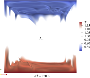
  $Ra$ are provided in the supplementary materials available at https://doi.org/10.1017/jfm.2020.66. It should be mentioned that the LSC can still be observed from the mean flow field in this case, but the mean velocity distribution is changed, which will be further discussed in the following. In figure 2(e,f) we show the volume rendering of 3-D temperature fields. Vigorous sheetlike plumes are emitted from the bottom and top plates, with no significant differences in plume structures between the OB and NOB cases. Overall, for air, we cannot observe obvious qualitative differences from the snapshots between OB and NOB cases for the same
  $Ra$, which is different from the NOB cases in water (Sugiyama et al. Reference Sugiyama, Calzavarini, Grossmann and Lohse2009).

Figure 2. Snapshots of the 2-D velocity (arrows) and reduced temperature  $\unicode[STIX]{x1D6E9}$ (colour) fields for
  $Pr=0.71$ with different
  $\unicode[STIX]{x1D716}$ and
  $Ra$. (a,b)
  $Ra=5\times 10^{8}$; (a) OB, (b)
  $\unicode[STIX]{x1D716}=0.2$. (c,d)
  $Ra=8\times 10^{8}$; (c) OB, (d)
  $\unicode[STIX]{x1D716}=0.2$. (e,f) Volume rendering of 3-D temperature fields (
 $T$) for
  $Ra=10^{7}$; (e) OB, (f)
  $\unicode[STIX]{x1D716}=0.2$.

Figure 3. Mean velocity profiles of  $\bar{v}(z)$ for 2-D cases in the plane of
  $y=0.5$ (a,b) and
  $\bar{w}(y)$ in the plane of
  $z=0.5$ (c,d) for (a,c)
  $Ra=10^{8}$ and (b,d)
  $Ra=10^{9}$.
To better show NOB effects on the velocity field, we present in figure 3 the mean horizontal velocity profiles  $\bar{v}(z)$ at
  $y=0.5$ and mean vertical velocity profiles
  $\bar{w}(y)$ at
  $z=0.5$ for
  $Ra=10^{8}$ and
  $10^{9}$ in OB and various
  $\unicode[STIX]{x1D716}$ in 2-D cases, respectively. Due to the inherent nature of top-down symmetry breaking, the flow structures will be asymmetric as stated in (Zhang et al. Reference Zhang, Childress and Libchaber1997). From figure 3, we can see that the profiles of the horizontal velocity
  $\bar{v}(z)$ and the vertical velocity
  $\bar{w}(y)$ become asymmetric to a certain degree. It should be mentioned that the profiles at
  $Ra=10^{9}$ shown in figure 3(b) are different from those at
  $Ra=10^{8}$ shown in figure 3(a), due to the change of flow pattern as illustrated in figure 2. At
  $Ra=10^{8}$, there is a relatively stable LSC, giving rise to the peaks of the profile near the edge of the top/bottom viscous BL. However, at
  $Ra=10^{9}$, the stable LSC is broken and there are large vortices detached from corner rolls, and the convection of those large vortices has led the peaks of the profile occurring in the bulk (e.g.
  $z\simeq 0.2$ at the bottom) rather than the edge of the viscous BL. Interestingly, even without stable LSC in this case, we can still find the BL structures and a relatively sharp transition of the velocity profiles occurring near the edge of the viscous BL. In § 3.4 we will further discuss the NOB effects on the profiles of the viscous BLs, which can be described qualitatively by laminar BL theory.

Figure 4. Graphs of  $\bar{v}_{r}$ (a) and
  $\bar{w}_{r}$ (b) versus
  $Ra$ for different
  $\unicode[STIX]{x1D716}$ for 2-D cases.
In order to quantify the intensity of velocity asymmetry, for 2-D cases, the absolute value of the ratio of horizontal maximum mean velocity  $\bar{v}_{max}$ and horizontal minimum mean velocity
  $\bar{u}_{min}$ is calculated, namely,
  $\bar{v}_{r}=|\bar{v}_{max}|/|\bar{v}_{min}|$, and a similar ratio is also obtained for the vertical velocity
  $\bar{w}_{r}=|\bar{w}_{max}|/|\bar{w}_{min}|$. In figure 4 we show
  $\bar{v}_{r}$ and
  $\bar{w}_{r}$ as a function of
  $Ra$ for different
  $\unicode[STIX]{x1D716}$. It is well known that the velocity ratios should be equal to 1 within OB approximation due to inherent symmetry of the system, while they deviate from 1 under NOB conditions. Here, we can see that
  $\bar{v}_{r}$ or
  $\bar{w}_{r}$ is a non-monotonic function of
  $Ra$ for different
  $\unicode[STIX]{x1D716}$. For
  $Ra\lesssim 8\times 10^{8}$,
  $\bar{v}_{r}$ shows a strong deviation under NOB conditions, and the maximum deviation is around
  $8\,\%$ at
  $Ra=3\times 10^{8}$ with
  $\unicode[STIX]{x1D716}=0.4$. Similar behaviors are found for
  $\bar{w}_{r}$. Furthermore, the most interesting feature is that the
  $Ra$ dependence of
  $\bar{v}_{r}$ or
  $\bar{w}_{r}$ is not monotonous, similar to the convection of air with NOB effects in a differentially heated cell (Wang et al. Reference Wang, Xia, Yan, Sun and Wan2019a). Based on the present data, it seems that the asymmetric feature of velocity is weakened for high
  $Ra$, which should also be attributed to the change of flow pattern when
  $Ra\gtrsim 8\times 10^{8}$, as illustrated in figure 2.
3.1.2 The temperature profiles and shift of centre temperature
Apart from the velocity distribution, the NOB effects also exert a significant influence on the temperature field. Here, we are committed to studying the influence of NOB effects on temperature profiles and centre temperature quantitatively. Within OB approximation, the centre temperature  $T_{c}$ should be equal to 1 (or
  $\unicode[STIX]{x1D6E9}_{c}=0$). However, the
  $T_{c}$ measured under NOB conditions will deviate from this mean value, due to the asymmetry between top and bottom thermal BLs (Ahlers et al. Reference Ahlers, Araujo, Funfschilling, Grossmann and Lohse2007; Sugiyama et al. Reference Sugiyama, Calzavarini, Grossmann and Lohse2009; Horn et al. Reference Horn, Shishkina and Wagner2013; Weiss et al. Reference Weiss, He, Ahlers, Bodenschatz and Shishkina2018). For instance, with much smaller
  $\unicode[STIX]{x1D707}/k$, the thicknesses of viscous/thermal BLs near the cold wall become much thinner in the present system (Xia et al. Reference Xia, Wan, Liu, Wang and Sun2016).

Figure 5. The profiles of time-averaged reduced temperatures  $\langle \unicode[STIX]{x1D6E9}\rangle _{t}$ for 2-D cases at
 $y=0.5$ for (a)
  $Ra=10^{8}$ and (b)
  $Ra=10^{9}$.

Figure 6. (a) The profiles of time- and plane-averaged reduced temperatures  $\langle \unicode[STIX]{x1D6E9}\rangle _{t,S}$ for a 3-D case at
  $Ra=10^{8}$. Panels (b) and (c) are the local enlargement of (a).
In figure 5 we show the profiles of time-averaged reduced temperatures  $\langle \unicode[STIX]{x1D6E9}\rangle _{t}$ on the line at
  $y=0.5$ in 2-D OB and NOB cases with different
  $\unicode[STIX]{x1D716}$ and
  $Ra$. For OB cases,
  $\unicode[STIX]{x1D6E9}$ in the bulk is nearly zero, and slight overshoots are observed near the edge of the thermal BL for
  $Ra=10^{8}$, which is influenced by the relatively large size corner rolls. Such overshoots can also be observed in NOB cases. At
  $Ra=10^{9}$, the overshoots disappear since these corner rolls are smaller and detach from the corner frequently. For NOB cases,
  $\unicode[STIX]{x1D6E9}$ in the bulk become positive for various
  $\unicode[STIX]{x1D716}$ and
  $Ra$. This finding is similar to that in strongly turbulent RB convection in liquids (Ahlers et al. Reference Ahlers, Brown, Araujo, Funfschilling, Grossmann and Lohse2006), which is opposed to the previous finding for ethane gas close to its critical point (Ahlers et al. Reference Ahlers, Araujo, Funfschilling, Grossmann and Lohse2007). It should be mentioned that the prediction of the central temperature is still a tough task because of the nonlinear temperature dependence of material properties. In the present system, the thermal conductivity increases with the increase in temperature, similar to that in liquids instead of gaseous ethane close to its critical point, which might play a dominant role. In figure 6 we show the profiles of time- and plane-averaged reduced temperatures
  $\langle \unicode[STIX]{x1D6E9}\rangle _{t,S}$ for the 3-D case at
  $Ra=10^{8}$ for various
  $\unicode[STIX]{x1D716}$. The asymmetry of top and bottom thermal BLs is still presented under NOB conditions, but the shift of
  $T_{c}$ in the bulk becomes much smaller. At
  $z/H=0.5$, the centre reduced temperature
  $\unicode[STIX]{x1D6E9}_{c}$ is of the order
  $10^{-3}$, which is almost close to the level of statistical uncertainties. The NOB effects on the shift of
  $T_{c}$ are greatly reduced in 3-D cases, which has not been fully understood. We guess that it might be attributed to better fluid mixing for air in the bulk with the flow motion in the third dimension.

Figure 7. (a) Variations of  $k$ with
  $\unicode[STIX]{x1D6E9}$. (b) The profiles of
  $\unicode[STIX]{x1D6E9}$ for OB and various
  $\unicode[STIX]{x1D716}$ cases at the motionless state.
In the present cases, we conjecture that the positive shift of  $T_{c}$ is mainly attributed to the temperature-dependent thermal conductivity
  $k$. In other word, the sign of
  $\unicode[STIX]{x1D6E9}_{c}$ can be judged beforehand based on the solution of the motionless state as follows. It is well known that the motionless conductive state is always a solution of the system before convection onset, which can be used as the base flow for studying onset of instability (Liu et al. Reference Liu, Xia, Yan, Wan and Sun2018). With fixed temperatures at the top and bottom boundaries, the profiles of temperature
  $T$ for different
  $\unicode[STIX]{x1D716}$ can be obtained by solving the nonlinear equation
 $$\begin{eqnarray}\frac{\text{d}}{\text{d}z}\left(k\frac{\text{d}T}{\text{d}z}\right)=0,\end{eqnarray}$$
with given boundary conditions at the top and bottom plates
 $$\begin{eqnarray}T|_{z=H}=1-\unicode[STIX]{x1D716},\quad T|_{z=0}=1+\unicode[STIX]{x1D716}.\end{eqnarray}$$
 In figure 7(a) we show the thermal conductivity  $k$ as a function of
  $\unicode[STIX]{x1D6E9}$, while the profiles of temperature in the conduction state in the OB and NOB cases are presented in figure 7(b). It is seen that
  $T_{c}$ will always be higher than 1 in the present cases, which is qualitatively in consistence with the present DNS results shown in figure 5. The shifts of
  $T_{c}$ at the cell centre under motionless states are around 0.022, 0.044 and 0.087 for
  $\unicode[STIX]{x1D716}=0.1,0.2$ and
  $0.4$, respectively, which will be compared with DNS results with turbulent convection at relatively high
  $Ra$.
$Ra$.

Figure 8. (a) The relative deviations versus  $\unicode[STIX]{x1D716}$ for air for various
  $Ra$ in 2-D cases. (b) The relative deviations as a function of
  $Ra$ for various
  $\unicode[STIX]{x1D716}$ in 2-D cases.

Figure 9. The time-averaged temperature  $(T-T_{m})/2\unicode[STIX]{x1D716}$ fields at (a)
  $Ra=5\times 10^{8}$ and (b)
  $Ra=10^{9}$ under NOB conditions. The mean velocity vectors are also shown.
As mentioned before, the shift of  $T_{c}$ is greatly reduced in 3-D cases; thus, in figure 8(a) we only show the relative deviation
  $(T_{c}-T_{m})/2\unicode[STIX]{x1D716}$ at the cell centre versus
  $\unicode[STIX]{x1D716}$ at various
  $Ra$ in 2-D cases. We can see that all deviations are positive, in qualitative agreement with predictions under motionless states as shown in figure 7. This is similar to the finding for water (Sugiyama et al. Reference Sugiyama, Calzavarini, Grossmann and Lohse2009). Moreover, the
  $T_{c}$ is strongly dependent on
  $Ra$, and the maximum relative deviation is about
  $5\,\%$, occurring at
  $Ra=3\times 10^{8}$, but all the relative deviations are below the values of the motionless states. Previously, for convection in water under NOB conditions, Sugiyama et al. (Reference Sugiyama, Calzavarini, Grossmann and Lohse2009) found that the relative deviation is rather independent of
  $Ra$ as
  $Ra\gtrsim 10^{5}$ and it almost increases linearly with increasing temperature difference. However, for 2-D RB convection of air with a large temperature difference, the data points of relative deviations are quite scattered, and such a linear relationship seems to be no longer valid. Furthermore, for RB convection in water with NOB effects, the
  $T_{c}$ can even be reasonably predicted by the extended Prandtl–Blasius BL theory (Ahlers et al. Reference Ahlers, Brown, Araujo, Funfschilling, Grossmann and Lohse2006) despite the large deviations in the temperature profiles. Nevertheless, due to the strong scatter and
  $Ra$ dependence of our data, we cannot directly borrow the extended BL theory to predict
  $T_{c}$ in the present cases. In figure 8(b) we show relative deviations versus
  $\unicode[STIX]{x1D716}$ for different
  $Ra$. Clearly, the largest deviations occur at
  $\unicode[STIX]{x1D716}=0.4$ for all
  $Ra$ numbers. Similar to
  $\bar{v}_{r}$ or
  $\bar{w}_{r}$, the
  $Ra$ dependence of
  $T_{c}$ is not monotonous. Interestingly, for
  $Ra\gtrsim 5\times 10^{8}$, the value of relative deviation will not be enhanced, but reduced slightly for all
  $\unicode[STIX]{x1D716}$ as
  $Ra$ increases, which might be attributed to the altered flow organizations. In figure 9 we show the mean temperature fields
  $(T-T_{m})/2\unicode[STIX]{x1D716}$ at
  $Ra=5\times 10^{8}$ and
  $10^{9}$. It is clear that the size of the corner roll is smaller at
  $Ra=10^{9}$ than at
  $Ra=5\times 10^{8}$, and the former case has a smaller value of
  $(T_{c}-T_{m})/2\unicode[STIX]{x1D716}$. The mean flow organization at
  $Ra=10^{9}$ for the
  $\unicode[STIX]{x1D716}=0.1$ case is quite similar to that for the
  $\unicode[STIX]{x1D716}=0.2$ case, and then we can see that their values of
  $(T_{c}-T_{m})/2\unicode[STIX]{x1D716}$ are very close, as shown in figure 8(b). The
  $\unicode[STIX]{x1D716}=0.4$ case at
  $Ra=10^{9}$ has a larger hot left-bottom corner roll, which produces a larger relative deviation at the cell centre. Thus, except for the boundary layers, we think the flow organization also plays a certain role in determining the relative deviation at the cell centre.
3.2 Global heat transport
We now pay attention to the global heat transport with and without NOB effects, which is measured by the Nusselt number  $Nu$, defined as
 $$\begin{eqnarray}Nu=\frac{Q}{k2\unicode[STIX]{x1D716}/H},\end{eqnarray}$$
 where  $Q$ is the heat flux across any horizontal plane. In figures 10(a) and 10(c) we show the log–log plot of
  $Nu$ versus
  $Ra$ for OB and NOB cases for various
  $\unicode[STIX]{x1D716}$. It is clear that the change of
  $Nu$ caused by NOB effects is quite small, which cannot be distinguished directly in a log–log plot. Therefore, we list the raw data of
  $Nu$ for all cases in tables 3 and 4. It is well known that in RB convection for a fixed
  $Pr$, the relationship between
  $Nu$ and
  $Ra$ can usually be expressed by a power-law scaling, i.e.
  $Nu\sim Ra^{\unicode[STIX]{x1D6FC}}$. For 2-D RB convection within OB approximation, Zhang, Zhou & Sun (Reference Zhang, Zhou and Sun2017) examined
  $Ra$ scalings of
  $Nu$ for
  $Pr=0.7$ and
  $Pr=5.3$, which yielded
  $Nu\sim Ra^{0.30\pm 0.02}$ for both
  $Pr$. Presently, in table 1 we list the best power-law fitting to
  $Nu$ versus
  $Ra$ for OB and various
  $\unicode[STIX]{x1D716}$ cases. Clearly, for current 2-D cases in the
  $Ra$ number range
  $5\times 10^{7}\leqslant Ra\leqslant 5\times 10^{9}$, the
  $Nu$ versus
  $Ra$ for OB cases yields
  $Nu\sim Ra^{0.295}$, which is very close to that in (Johnston & Doering Reference Johnston and Doering2009; van der Poel et al. Reference van der Poel, Stevens, Sugiyama and Lohse2012; Zhang et al. Reference Zhang, Zhou and Sun2017; Wang et al. Reference Wang, Zhou, Wan and Sun2019b). It should be emphasized that the
  $Ra$-scaling exponents are also insensitive to NOB effects in RB convection despite the changes in flow organizations caused by top-down symmetry breaking, similar to the differentially heated cavity (Wang et al. Reference Wang, Xia, Yan, Sun and Wan2019a). For present 3-D cases in the
  $Ra$ number range
  $3\times 10^{6}\leqslant Ra\leqslant 10^{8}$, the
  $Nu$ versus
  $Ra$ for OB cases yields
  $Nu\sim Ra^{0.285}$, which is also close to its 2-D counterpart.

Figure 10. The Nusselt number  $Nu$ versus
  $Ra$ for OB and various
  $\unicode[STIX]{x1D716}$ for 2-D cases (a) and 3-D cases (c);
  $Nu_{NOB}/Nu_{OB}$ versus
  $\unicode[STIX]{x1D716}$ for various
  $Ra$ in (b) 2-D cases and (d) 3-D cases. The dashed lines are power-law fitting for OB data.
Table 1. The best power-law fit of  $Nu\sim Ra^{\unicode[STIX]{x1D6FC}}$ for OB and various
  $\unicode[STIX]{x1D716}$ cases in 2-D and 3-D cases.

In addition, to quantitatively show the NOB effects on  $Nu$, the Nusselt number ratio
  $Nu_{NOB}/Nu_{OB}$ versus
  $\unicode[STIX]{x1D716}$ for all
  $Ra$ is shown in figures 10(b,d). As previously mentioned, the flow organizations are changed due to NOB effects, including the mean velocity and temperature profiles. However, the Nusselt number
  $Nu$ seems to be insensitive to changes in
  $\unicode[STIX]{x1D716}$, even up to
  $\unicode[STIX]{x1D716}=0.4$, corresponding to the dimensional temperature difference 240 K. For 2-D cases, the maximum deviation of
  $Nu_{NOB}/Nu_{OB}$ from 1 for all
  $Ra$ is less than
  $2\,\%$. It is also found that the maximum deviation for 3-D cases (
 ${\lesssim}1\,\%$) is even smaller than that for 2-D cases. Interestingly, similar to
  $Ra$ dependence of
  $T_{c}$, the Nusselt number ratios display an obvious dependence on
  $Ra$ in spite of the limited deviations, while they are only weakly dependent on
  $Ra$ for water with NOB effects (Sugiyama et al. Reference Sugiyama, Calzavarini, Grossmann and Lohse2009).
3.3 Reynolds numbers
In RB convection, the Reynolds number  $Re$ is an important response parameter, which is defined as
 $$\begin{eqnarray}Re=\frac{\hat{U} {\hat{H}}}{\hat{\unicode[STIX]{x1D708}_{0}}}=\sqrt{\frac{Ra}{Pr}}U,\end{eqnarray}$$
 where  $\hat{U}$ and
  $U$ are the dimensional and dimensionless characteristic velocities.
Here, we choose the root mean square (r.m.s.) velocities as the characteristic velocity (Wagner & Shishkina Reference Wagner and Shishkina2013; Zhang et al. Reference Zhang, Zhou and Sun2017, Reference Zhang, Sun, Bao and Zhou2018; Ng et al. Reference Ng, Ooi, Lohse and Chung2018), i.e.  $U=U^{rms}=\sqrt{\langle \boldsymbol{u}\boldsymbol{\cdot }\boldsymbol{ u}\rangle _{V}}$, where
  $\langle \boldsymbol{\cdot }\rangle _{V}$ denotes the space average in two and three dimensions and
  $\boldsymbol{u}$ is the velocity vector. In figure 11(a,c) we show
  $Re$ based on r.m.s. of velocities as a function of
  $Ra$ for OB and NOB for various
  $\unicode[STIX]{x1D716}$. Similar to
  $Nu$, the Reynolds number can also be expressed by a power-law scaling, i.e.
  $Re\sim Ra^{\unicode[STIX]{x1D6FD}}$, as shown in table 2. It is clear that the influence of NOB effects on
  $Re$ are quite limited, which almost has no influence on the
  $Ra$ scaling exponents. Based on
  $U^{rms}$, the power-law fitting to the data of OB cases yields the scaling of
  $Re\sim Ra^{0.617}$ in 2-D cases and
  $Re\sim Ra^{0.491}$ in 3-D cases. For 2-D cases, the scaling exponent 0.617 is in excellent agreement with the exponent 0.62 found for the OB case of water by Sugiyama et al. (Reference Sugiyama, Calzavarini, Grossmann and Lohse2009), and is also close to 0.6 reported by Zhang et al. (Reference Zhang, Zhou and Sun2017) and Wang et al. (Reference Wang, Zhou, Wan and Sun2019b) recently. For 3-D cases, the scaling exponent is notably smaller than that for 2-D RB flows, which agrees with previous findings that this exponent ranges from 0.42 to 0.5 for 3-D RB flows with various working fluids based on one- and multiple-point measurements (Niemela et al. Reference Niemela, Skrbek, Sreenivasan and Donnelly2001; Qiu & Tong Reference Qiu and Tong2001; Sun & Xia Reference Sun and Xia2005; Brown, Funfschilling & Ahlers Reference Brown, Funfschilling and Ahlers2007). To show the differences quantitatively due to NOB effects, the Reynolds number ratio
  $Re_{NOB}/Re_{OB}$ versus
  $\unicode[STIX]{x1D716}$ for all
  $Ra$ is presented in figure 11(b,d). We note that the maximum deviation of
  $Re_{NOB}/Re_{OB}$ from 1 for all
  $Ra$ numbers is about
  $3\,\%$ for 2-D cases and about
  $1\,\%$ for 3-D cases. In the scope of the present data, this deviation does not show an obvious growth trend with increasing
  $Ra$ or
  $\unicode[STIX]{x1D716}$, so we guess that the NOB effects at some higher
  $Ra$ experiments might also be limited at least for air.
Table 2. The best power-law fittings for  $Re$ versus
  $Ra$ for OB and various
  $\unicode[STIX]{x1D716}$ in 2-D and 3-D cases.


Figure 11. The Reynolds number  $Re^{rms}$ based on the root mean square (r.m.s.) velocities versus
  $Ra$ for OB and NOB with various
  $\unicode[STIX]{x1D716}$ in (a) 2-D and (c) 3-D cases. The error bars are smaller than the symbol sizes. The dashed lines are the best power-law fit for OB data. The Reynolds number ratio
  $Re_{NOB}/Re_{OB}$ versus
  $\unicode[STIX]{x1D716}$ at various
  $Ra$ numbers for (b) 2-D and (d) 3-D cases.
3.4 The viscous and thermal boundary layers
The viscous and thermal BLs play an essential role in global heat transport across the fluid layer (Grossmann & Lohse Reference Grossmann and Lohse2000). The Nusselt number is related, directly or intimately, to the thickness of the thermal BLs, due to the fact that within the thermal BLs heat is mainly transported via conduction (Wu & Libchaber Reference Wu and Libchaber1991; Belmonte, Tilgner & Libchaber Reference Belmonte, Tilgner and Libchaber1994; Lui & Xia Reference Lui and Xia1998). In this section, we are committed to studying the viscous and thermal BLs with strong variations of density, as well as  $\unicode[STIX]{x1D707}$ and
  $k$. The NOB effects on flow structures and heat transport are more significant in 2-D RB flows; thus, we mainly discuss the results for 2-D cases below.
3.4.1 The extended BL equations for air with a large temperature difference
Here, we derive the laminar BL equations starting from the non-dimensionalized low-Mach-number Navier–Stokes equations. For derivation of a steady BL solution, we assume time derivatives to be zero ( $\unicode[STIX]{x2202}(\cdot )/\unicode[STIX]{x2202}t\equiv 0$) in (2.1)–(2.3). Furthermore, we consider a 2-D BL in the
  $x{-}z$ plane with a zero-pressure gradient, and the buoyancy term is neglected. The temperature is assumed to be advected passively. Finally, the equations of flow motion are simplified to
 $$\begin{eqnarray}\displaystyle & \displaystyle \frac{\unicode[STIX]{x2202}\unicode[STIX]{x1D70C}u}{\unicode[STIX]{x2202}x}+\frac{\unicode[STIX]{x2202}\unicode[STIX]{x1D70C}w}{\unicode[STIX]{x2202}z}=0, & \displaystyle\end{eqnarray}$$
 $$\begin{eqnarray}\displaystyle & \displaystyle \unicode[STIX]{x1D70C}u\frac{\unicode[STIX]{x2202}u}{\unicode[STIX]{x2202}x}+\unicode[STIX]{x1D70C}w\frac{\unicode[STIX]{x2202}u}{\unicode[STIX]{x2202}z}=\sqrt{\frac{Pr}{Ra}}\frac{\unicode[STIX]{x2202}}{\unicode[STIX]{x2202}z}\left(\unicode[STIX]{x1D707}\frac{\unicode[STIX]{x2202}u}{\unicode[STIX]{x2202}z}\right), & \displaystyle\end{eqnarray}$$
 $$\begin{eqnarray}\displaystyle & \displaystyle \unicode[STIX]{x1D70C}C_{p}\left(u\frac{\unicode[STIX]{x2202}T}{\unicode[STIX]{x2202}x}+w\frac{\unicode[STIX]{x2202}T}{\unicode[STIX]{x2202}z}\right)=\frac{1}{\sqrt{RaPr}}\frac{\unicode[STIX]{x2202}}{\unicode[STIX]{x2202}z}\left(k\frac{\unicode[STIX]{x2202}T}{\unicode[STIX]{x2202}z}\right). & \displaystyle\end{eqnarray}$$
 Here we further assume that  $\unicode[STIX]{x1D70C}T=1,$ which is valid for open systems. Furthermore, we introduce a stream function:
 $$\begin{eqnarray}\unicode[STIX]{x1D70C}u=\frac{\unicode[STIX]{x2202}\unicode[STIX]{x1D6F9}}{\unicode[STIX]{x2202}z},\quad \unicode[STIX]{x1D70C}w=-\frac{\unicode[STIX]{x2202}\unicode[STIX]{x1D6F9}}{\unicode[STIX]{x2202}x}.\end{eqnarray}$$
 Next, referring to Ahlers et al. (Reference Ahlers, Brown, Araujo, Funfschilling, Grossmann and Lohse2006, Reference Ahlers, Araujo, Funfschilling, Grossmann and Lohse2007), we further introduce a self-similar variable  $\tilde{Z}=z/L$, while
  $\widetilde{\unicode[STIX]{x1D6F9}}=\unicode[STIX]{x1D6F9}/LU$, such that
  $L=(Pr/Ra)^{1/4}\sqrt{x/U}$. So the velocity components become
 $$\begin{eqnarray}u=\frac{U}{\unicode[STIX]{x1D70C}}\tilde{\unicode[STIX]{x1D6F9}^{\prime }},\quad w=\sqrt{\frac{Pr}{Ra}}\frac{1}{2\unicode[STIX]{x1D70C}L}(\tilde{Z}\tilde{\unicode[STIX]{x1D6F9}^{\prime }}-\tilde{\unicode[STIX]{x1D6F9}}).\end{eqnarray}$$
Then, the momentum equation becomes
 $$\begin{eqnarray}\unicode[STIX]{x1D707}\tilde{\unicode[STIX]{x1D6F9}}^{\prime \prime \prime }+\left(\frac{\tilde{\unicode[STIX]{x1D6F9}}}{2}-\unicode[STIX]{x1D707}\frac{2\unicode[STIX]{x1D70C}^{\prime }}{\unicode[STIX]{x1D70C}}+\unicode[STIX]{x1D707}^{\prime }\right)\tilde{\unicode[STIX]{x1D6F9}}^{\prime \prime }+\left[\unicode[STIX]{x1D707}\left(\frac{2\unicode[STIX]{x1D70C}^{\prime }\unicode[STIX]{x1D70C}^{\prime }}{\unicode[STIX]{x1D70C}^{2}}-\frac{\unicode[STIX]{x1D70C}^{\prime \prime }}{\unicode[STIX]{x1D70C}}\right)-\unicode[STIX]{x1D707}^{\prime }\frac{\unicode[STIX]{x1D70C}^{\prime }}{\unicode[STIX]{x1D70C}}-\frac{\tilde{\unicode[STIX]{x1D6F9}}}{2}\frac{\unicode[STIX]{x1D70C}^{\prime }}{\unicode[STIX]{x1D70C}}\right]\tilde{\unicode[STIX]{x1D6F9}}^{\prime }=0,\end{eqnarray}$$
and the temperature equation becomes
 $$\begin{eqnarray}kT^{\prime \prime }+(k^{\prime }+{\textstyle \frac{1}{2}}C_{p}Pr\tilde{\unicode[STIX]{x1D6F9}})T^{\prime }=0.\end{eqnarray}$$
 From the equation of state  $\unicode[STIX]{x1D70C}=1/T$, we obtain
 $$\begin{eqnarray}\displaystyle & \displaystyle \unicode[STIX]{x1D707}\tilde{\unicode[STIX]{x1D6F9}}^{\prime \prime \prime }+\left(\frac{\tilde{\unicode[STIX]{x1D6F9}}}{2}+\unicode[STIX]{x1D707}\frac{2T^{\prime }}{T}+\unicode[STIX]{x1D707}^{\prime }\right)\tilde{\unicode[STIX]{x1D6F9}}^{\prime \prime }+\left(\unicode[STIX]{x1D707}\frac{T^{\prime \prime }}{T}+\unicode[STIX]{x1D707}^{\prime }\frac{T^{\prime }}{T}+\frac{1}{2}\tilde{\unicode[STIX]{x1D6F9}}\frac{T^{\prime }}{T}\right)\tilde{\unicode[STIX]{x1D6F9}}^{\prime }=0, & \displaystyle\end{eqnarray}$$
 $$\begin{eqnarray}\displaystyle & \displaystyle kT^{\prime \prime }+(k^{\prime }+{\textstyle \frac{1}{2}}C_{p}Pr\tilde{\unicode[STIX]{x1D6F9}})T^{\prime }=0, & \displaystyle\end{eqnarray}$$
where
 $$\begin{eqnarray}\displaystyle & \displaystyle \unicode[STIX]{x1D707}^{\prime }=(1+S_{\unicode[STIX]{x1D707}})\left(-\frac{T^{1.5}}{(T+S_{\unicode[STIX]{x1D707}})^{2}}+\frac{1.5T^{0.5}}{(T+S_{\unicode[STIX]{x1D707}})}\right)T^{\prime }, & \displaystyle\end{eqnarray}$$
 $$\begin{eqnarray}\displaystyle & \displaystyle k^{\prime }=(1+S_{k})\left(-\frac{T^{1.5}}{(T+S_{k})^{2}}+\frac{1.5T^{0.5}}{(T+S_{k})}\right)T^{\prime }, & \displaystyle\end{eqnarray}$$
and the boundary conditions
 $$\begin{eqnarray}\unicode[STIX]{x1D6F9}(0)=0,\quad \unicode[STIX]{x1D6F9}^{\prime }(0)=0,\quad \unicode[STIX]{x1D6F9}^{\prime }(\infty )=\unicode[STIX]{x1D70C}_{\infty },\end{eqnarray}$$
 $$\begin{eqnarray}T(0)=T_{w},\quad T(\infty )=T_{\infty }.\end{eqnarray}$$
 In this paper, we use the density and temperature at the cell centre from DNS results to define the boundary conditions for the BL equations at infinity ( $\unicode[STIX]{x1D70C}_{\infty },T_{\infty }$). Here,
  $T_{w}$ is the temperature at the wall as sketched in figure 1, i.e.
  $T_{w}=1+\unicode[STIX]{x1D716}$ (hot plate) or
  $T_{w}=1-\unicode[STIX]{x1D716}$ (cold plate). Then, the new BL equations can be solved by the shooting method, the results of which are compared to the DNS results in § 3.4.2.

Figure 12. The definition of the thickness of viscous BL for DNS results, where the OB case at  $Ra=10^{9}$ is used. The edge of BL (red dot) with velocity
  $v_{e}$ is defined at the position of
  $3\,\%$ of the peak value of the secondary derivative of velocity
  $|v^{\prime \prime }(z)|$.
3.4.2 The viscous/thermal boundary layer
Here, in some cases, we cannot find the maximum velocity near the BL edge as shown in figure 3(b). Therefore, we use a new definition of the thickness of the viscous BL ( $\unicode[STIX]{x1D6FF}_{v}$) as illustrated in figure 12, which is slightly different from that in prior studies (Sun, Cheung & Xia Reference Sun, Cheung and Xia2008; Wei & Xia Reference Wei and Xia2013). According to BL theory, the viscous effects mainly come from the term containing the secondary derivative of velocity. In order to find the edge of the viscous BL, we calculate the secondary derivative of velocity with respect to
  $z$, i.e.
  $v^{\prime \prime }(z)$, and set the location of 3 % of the peak value of
  $|v^{\prime \prime }(z)|$ to be the edge of the viscous BL, ensuring that the viscous effects become small at this location and beyond. Then, the velocity at the edge of the viscous BL is denoted as
  $v_{e}$. The thickness of the viscous BL
  $\unicode[STIX]{x1D6FF}_{v}$ is defined as the distance from the wall at which the extrapolation of the linear part of the horizontal velocity profile meets the horizontal line passing through the velocity
  $v_{e}$. We examined that, for
  $Ra=10^{8}$, this difference of
  $\unicode[STIX]{x1D6FF}_{v}$ between current and prior definitions is less than 1 %. The thickness of the thermal BL (
 $\unicode[STIX]{x1D6FF}_{T}$) can also be defined using the centre temperature
  $T_{c}$ in a similar way (Zhou & Xia Reference Zhou and Xia2013).

Figure 13. The comparison of normalized velocity profiles of current BL equations and DNS results for OB and NOB cases with different  $Ra$ on the line
  $y=0.5$. (a,b)
  $Ra=10^{8}$, (c,d)
  $Ra=10^{9}$. (a,c) The BL profiles on the bottom plate. (b,d) The BL profiles on the top plate. Here,
  $\unicode[STIX]{x1D6FF}_{v}$ is the thickness of the viscous BL and
  $u_{e}$ is the velocity at the edge of the BL.
In figure 13 we show the profiles of normalized velocity  $v(z)/v_{e}$ as a function of
  $z/\unicode[STIX]{x1D6FF}_{v}$ for
  $Ra=10^{8},10^{9}$ for OB and NOB cases on the line
  $y=0.5$ in 2-D cases. For each DNS case, the combination of
  $v_{e}$ and
  $\unicode[STIX]{x1D6FF}_{v}$ can be uniquely determined. Due to symmetry breaking under NOB conditions, the velocity profile on the bottom (top, respectively) plate is shown in figure 13(a,c) (figure 13b,d, respectively). There are some deviations of the velocity profile between the solutions of the present BL equations and DNS which are also found in experiments by (Wei & Xia Reference Wei and Xia2013), and DNS by (Shi, Emran & Schumacher Reference Shi, Emran and Schumacher2012). However, we find a similar trend of viscous BL profiles due to NOB effects between the extended BL solutions and DNS. Clearly, we find that the changes of the normalized velocity profiles on the bottom plate and the top plate are opposite. The deviations could result from the generation of plumes, pressure gradient and time variation of the BL, since the laminar BL theory relies on a series of assumptions. However, in general, our extended BL equations can reasonably predict the influence of NOB effects on the velocity profiles, regardless of the
  $Ra$. In figure 14 we further show the profiles of
  $\unicode[STIX]{x1D6E9}$ as a function of
  $z/\unicode[STIX]{x1D6FF}_{T}$ for
  $Ra=10^{8},10^{9}$ for both OB and NOB cases. The value of
  $\unicode[STIX]{x1D6FF}_{T}$ for each DNS case is determined according to
  $\unicode[STIX]{x1D6FF}_{v}$, since equations (3.10) and (3.11) are coupled. Again, the temperature profiles obtained by extended BL equations agree qualitatively with the DNS results, and we still observe a certain degree of deviations near the edge of thermal BLs.

Figure 14. The comparison of normalized temperature profiles of BL theory and DNS results as a function of  $z/\unicode[STIX]{x1D6FF}_{T}$ for OB and NOB cases with different
  $Ra$. (a,b)
  $Ra=10^{8}$, (c,d)
  $Ra=10^{9}$. (a,c) The temperature profiles on the bottom plate. (b,d) The temperature profiles on the top plate.
  $\unicode[STIX]{x1D6FF}_{T}$ is the thickness of thermal BL.

Figure 15. The compensation of viscous and thermal BLs. (a)  $F_{\unicode[STIX]{x1D6FF}_{v}}$ and (b)
  $F_{\unicode[STIX]{x1D6FF}_{T}}$ versus
  $Ra$ for various
  $\unicode[STIX]{x1D716}$ for 2-D cases on the line at
  $y=0.5$.
As shown in figure 13, we easily find that the thickness of the viscous/thermal BL is increased near the hot plate due to NOB effects, and decreased near the cold plate. In figure 15 we compare the sum of thicknesses of the top and bottom viscous/thermal BL for the NOB case to the OB case by calculating the ratios  $F_{\unicode[STIX]{x1D6FF}_{v}}$ and
  $F_{\unicode[STIX]{x1D6FF}_{T}}$ at
  $y=0.5$ for 2-D cases, which are defined as
 $$\begin{eqnarray}F_{\unicode[STIX]{x1D6FF}_{v}}=2\unicode[STIX]{x1D6FF}_{v}^{OB}/(\unicode[STIX]{x1D6FF}_{v}^{t}+\unicode[STIX]{x1D6FF}_{v}^{b})^{NOB};\quad F_{\unicode[STIX]{x1D6FF}_{T}}=2\unicode[STIX]{x1D6FF}_{T}^{OB}/(\unicode[STIX]{x1D6FF}_{T}^{t}+\unicode[STIX]{x1D6FF}_{T}^{b})^{NOB}.\end{eqnarray}$$
 From figure 15(a), it can be seen that there are relatively strong deviations from 1 for  $F_{\unicode[STIX]{x1D6FF}_{v}}$ (at most around 6 %), which are also
  $Ra$-dependent. For
  $Ra\lesssim 8\times 10^{8}$, the NOB effects on velocity fields are relatively stronger. For higher
  $Ra$, the LSC is broken, the corner rolls become unstable and the velocity fields are dominated by smaller vortex structures, which weaken the impact of NOB effects. In contrast to
  $F_{\unicode[STIX]{x1D6FF}_{v}}$, the NOB effects have less impact on
  $F_{\unicode[STIX]{x1D6FF}_{T}}$. The maximum deviation from 1 for
  $F_{\unicode[STIX]{x1D6FF}_{T}}$ is at most around 3 % due to cancellations between
  $\unicode[STIX]{x1D6FF}_{T}^{t}$ and
  $\unicode[STIX]{x1D6FF}_{T}^{b}$, close to the deviations of
  $Nu_{NOB}/Nu_{OB}$, but no tendency can be seen. In water under NOB conditions, Ahlers et al. (Reference Ahlers, Brown, Araujo, Funfschilling, Grossmann and Lohse2006) also attributed the robustness of
  $Nu$ towards NOB effects to a compensation effect of top and bottom thermal BLs. Present data for air – even with large temperature differences – seem to support this statement, suggesting that this mechanism holds in different systems under NOB conditions. As previously mentioned, the flow structure is reorganized around
  $Ra\simeq 8\times 10^{8}$ in 2-D cases, but one cannot observe any clear transition from the data of
  $F_{\unicode[STIX]{x1D6FF}_{T}}$.
4 Summary and conclusions
To summarize, we have systematically studied 2-D and 3-D RB convection of air under NOB conditions due to large temperature differences by DNS. We consider the turbulence system with large temperature differences (60 K–240 K), which gives rise in large density variations. The extremely large temperature difference case with  $\unicode[STIX]{x0394}\hat{T}=240$ K is also considered, which has not been reached in previous experiments. The strong NOB effects are induced in a moderate
  $Ra$ range
  $3\times 10^{6}\leqslant Ra\leqslant 5\times 10^{9}$. To the best of our knowledge, the low-Mach-number Navier–Stokes equations are firstly employed in order to treat 3-D turbulence with large density variations and temperature-dependent fluid properties in RB convection at relatively high
  $Ra$ (Livescu Reference Livescu2020).
Firstly, for air with large density variations, the top-down symmetry is broken with NOB effects which induces some changes in flow organizations, such as the shift of centre temperature  $T_{c}$ and the asymmetry of the velocity/thermal BLs. The
  $T_{c}$ is increased under NOB conditions compared to the arithmetic mean temperature of the top and bottom plates
  $T_{m}$, which is different from ethane gas close to its critical point (Ahlers et al. Reference Ahlers, Araujo, Funfschilling, Grossmann and Lohse2007). The maximum relative deviation
  $(T_{c}-T_{m})/2\unicode[STIX]{x1D716}$ is around 5 % in 2-D cases, while it becomes quite small in 3-D cases. As reported by Ahlers et al. (Reference Ahlers, Brown, Araujo, Funfschilling, Grossmann and Lohse2006) and Sugiyama et al. (Reference Sugiyama, Calzavarini, Grossmann and Lohse2009), the
  $T_{c}$ for water under NOB conditions are weakly dependent on
  $Ra$, which can be generally predicted by an extended Prandtl–Blasius theory. However, this theory fails in the present system due to the fact that present results of
  $T_{c}$ are scattered and strongly dependent on
  $Ra$. Combined with previous experimental and numerical results, we can conclude that the deviation of the centre temperature is sensitively dependent on the particular working fluid.
Moreover, for all  $Ra$ and
  $\unicode[STIX]{x1D716}$ explored, we find that the NOB effects have a very limited influence on
  $Nu$. The Nusselt number
  $Nu_{NOB}$ will differ from
  $Nu_{OB}$ by
  $2\,\%$ or less regardless of the existence of stable LSC. The Nusselt number ratios
  $Nu_{NOB}/Nu_{OB}$ are
  $Ra$- and
  $\unicode[STIX]{x1D716}$-dependent, while they are only weakly dependent on
  $Ra$ for water with NOB effects (Sugiyama et al. Reference Sugiyama, Calzavarini, Grossmann and Lohse2009; Demou & Grigoriadis Reference Demou and Grigoriadis2019). More importantly, we also find that the power-law scaling of
  $Nu\sim Ra^{\unicode[STIX]{x1D6FC}}$ is rather insensitive to the NOB effects. The maximum influence of NOB effects on
  $Re$ is around
  $3\,\%$ for 2-D cases and
  $1\,\%$ for 3-D cases, which are also
  $Ra$- and
  $\unicode[STIX]{x1D716}$-dependent. In general, the NOB effects on
  $Nu$ and
  $Re$ are much weaker in 3-D cases. This finding is also different from that for low-temperature gaseous helium (Sameen et al. Reference Sameen, Verzicco and Sreenivasan2008) in a 3-D cylindrical cell. Besides, unlike the NOB effects in water, the extremely large temperature differences induce large density variations, which is the most significant feature of the present system; however, the effects of large density variations seem to play a very limited role on global heat and momentum transport in the scope of the present study.
Finally, the extended BL equations based on low-Mach-number Navier–Stokes equations are developed, involving the strong variation of density, as well as the temperature-dependent fluid properties. The NOB effects on BL velocity profiles shown by DNS are predicted qualitatively by the extended BL theory in spite of the large deviations in the  $z$ dependence of horizontal mean velocity profiles on the line
  $y=0.5$ for 2-D cases. With increasing
  $\unicode[STIX]{x1D716}$, the relative velocity inside BLs near the hot plate is increased, while it decreases near the cold plate. From
  $F_{\unicode[STIX]{x1D6FF}_{v}}$ and
  $F_{\unicode[STIX]{x1D6FF}_{T}}$ data, we interestingly find that the NOB effects have a much stronger impact on the viscous BLs than the thermal BLs. For all
  $Ra$ explored, the
  $F_{\unicode[STIX]{x1D6FF}_{T}}$ data are scattered but their deviations from 1 are at most around 3 %, close to the deviations of
  $Nu_{NOB}/Nu_{OB}$. In the present system, the data also supports the fact that the compensation effect between the top and bottom thermal BL leads to the robustness of
  $Nu$ against the NOB effects, suggesting that this mechanism holds in many different systems under NOB conditions.
In a word, this study fills the gap of numerical study of NOB effects in air with large temperature differences at relatively high  $Ra$ in both 2-D and 3-D systems. The results show that the power-law scalings for
  $Nu$ and
  $Re$ versus
  $Ra$ are rather insensitive to the NOB effects for air, in particular for 3-D RB flows, which implies that the NOB effects may play a very limited role for
  $Nu$ and
  $Re$ at some high
  $Ra$ experiments with large temperature differences in air or other perfect gases.
Acknowledgements
This work is supported by the National Natural Science Foundation of China (NSFC) under grants 91952103, 11821202, 11825204 and 11621202, and the Fundamental Research Funds for the Central Universities. S.-N.X. thanks the fund of China Postdoctoral Science Foundation (2016M600306) and the NSFC under grant 11702167.
Declaration of interests
The authors report no conflict of interest.
Supplementary movies
Supplementary movies are available at https://doi.org/10.1017/jfm.2020.66.
Appendix. Details of the simulation parameters
The detailed simulation parameters and results are presented in tables 3 and 4.
Table 3. Simulation parameters for 2-D cases. The columns from left to right indicate the following: OB and various  $\unicode[STIX]{x1D716}$ cases (NOB); Rayleigh number
  $Ra$; grid size (
 $N_{x}\times N_{z}$); the averaging time for calculating statistics
  $t_{avg}$; the number of grid points within the bottom thermal BL
  $N_{BL}^{b}$; the number of grid points within the top thermal BL
  $N_{BL}^{t}$; Nusselt numbers
  $Nu$ measured at the bottom plate; Nusselt numbers
  $Nu_{V}=\sqrt{RaPr}\langle \unicode[STIX]{x1D716}_{u}\rangle _{V,t}+1$ measured by the globally averaged kinetic energy dissipation rates; and Reynolds numbers
  $Re=\sqrt{Ra/Pr}U^{rms}$. The Prandtl number
  $Pr$ is fixed to
  $0.71$.

Table 4. Simulation parameters for 3-D cases. The columns from left to right indicate the following: OB and various  $\unicode[STIX]{x1D716}$ cases (NOB); Rayleigh number
  $Ra$; grid size (
 $N_{x}\times N_{y}\times N_{z}$); the averaging time for calculating statistics
  $t_{avg}$; the number of grid points within the bottom thermal BL
  $N_{BL}^{b}$; the number of grid points within the top thermal BL
  $N_{BL}^{t}$; Nusselt numbers
  $Nu$ measured at the bottom plate; Nusselt numbers
  $Nu_{V}=\sqrt{RaPr}\langle \unicode[STIX]{x1D716}_{u}\rangle _{V,t}+1$ measured by the globally averaged kinetic energy dissipation rates; and Reynolds numbers
  $Re=\sqrt{Ra/Pr}U^{rms}$. The Prandtl number
  $Pr$ is fixed to
  $0.71$.


