2. Equations of motion

Our quasi-one-dimensional equations incorporate a couple assumptions: first, that motions transverse to the gradient of $r$ can be ignored; and second, that displacements are small enough ($\delta r\ll r_0$) that smooth functions of $r$ can be replaced with their values at $r_0$: for instance, $g=g_0$ and $A=A_0$. In addition, we neglect dissipative effects such as thermal diffusion; see Ro & Matzner (Reference Ro and Matzner2017) for a justification in the context of stellar outbursts.

We start with the conservation of mass,

(2.1)\begin{equation} d_t \ln \rho + A^{{-}1} \partial_r A v =0 , \end{equation}

and momentum,

(2.2)\begin{equation} d_t v + \frac1\rho \partial_r P ={-}g, \end{equation}

as well as background hydrostatic equilibrium,

(2.3)\begin{equation} \frac1\rho_0 \partial_{r_0} P_0 ={-}g_0. \end{equation}

We consider the fluid to be adiabatic and for simplicity we adopt an ideal gas equation of state,

(2.4)\begin{equation} P/P_0 = (\rho/\rho_0)^\gamma = x^\gamma, \end{equation}

where $\gamma$ may be a function of $r_0$.

We convert the spatial gradient ($\partial _r$) into gradients with respect to the initial radius ($\partial _{r_0}$) using $A \rho \, \textrm {d}r = A_0 \rho _0\, \textrm {d}r_0$, which implies

(2.5)\begin{equation} \rho^{{-}1} \partial_r = (A/A_0) \rho_0^{{-}1} \partial_{r_0} \simeq \rho_0^{{-}1} \partial_{r_0} \end{equation}

using $A\simeq A_0$. At the same time, we switch spatial variables from $r$ to $r_0$, allowing $d_t \rightarrow \partial _t$. Our equation for mass conservation becomes (using $r^{-1} \simeq r_0^{-1}$),

(2.6)\begin{equation} \partial_t \ln (\rho/\rho_0) + (\rho/\rho_0) \partial_{r_0} v + v \partial_{r_0} \ln A = 0. \end{equation}

The momentum equation becomes

(2.7)\begin{equation} \partial_t v + \frac1{\rho_0} \partial_{r_0} \delta P = 0 \end{equation}

or, using $P = x^\gamma P_0$ and writing out the derivative,

(2.8)\begin{equation} \partial_t v + \frac{\gamma P_0}{\rho_0} x^{\gamma-1} \partial_{r_0} x + \frac{\partial_{r_0} P_0}{\rho_0} (x^\gamma-1) + c_0^2 (\ln x)\partial_{r_0}\ln \gamma = 0, \end{equation}

which we re-write, using $\gamma P_0= \rho _0 c_0^2$, $\partial _{r_0} P_0 =- \rho _0 g_0$ and $c_0^2 x^{\gamma -1} = c^2$, as

(2.9)\begin{equation} \partial_t v + c^2 \partial_{r_0} x = (x^\gamma-1) g_0 - c_0^2(\ln x)\partial_{r_0}\ln \gamma. \end{equation}

The mass equation takes in the form

(2.10)\begin{equation} \partial_t x + x^2 \partial_{r_0} v ={-} v x \partial_{r_0} \ln A, \end{equation}

where we have multiplied through by $x$ to put the time derivatives in the same form as the momentum equation. Combining the momentum and mass equations,

(2.11)\begin{equation} \partial_t \boldsymbol{u} + {\boldsymbol{\mathsf{B}}}\, \partial_{r_0} \boldsymbol{u} = \boldsymbol{s}, \end{equation}

where

(2.12)\begin{equation} \boldsymbol{u} = \begin{pmatrix} v \\ x \end{pmatrix},\ \ \ {\boldsymbol{\mathsf{B}}} = \begin{bmatrix} 0 & c^2 \\ x^2 & 0 \end{bmatrix},\ \ \ \textrm{and}\ \ \ \boldsymbol{s} = \begin{pmatrix} (x^\gamma-1) g_0- c_0^2(\ln x)\partial_{r_0}\ln \gamma \\ - v x \partial_{r_0} \ln A \end{pmatrix}. \end{equation}

Note that our approximation of small radial perturbation only affects the form of $\boldsymbol {s}$.

3. Uniform planar case: Riemann invariants

In the simplest limit of a homogeneous background fluid and constant area, $g_0=0$ and $\partial _r \ln A=0$ so that $\boldsymbol {s}=0$. To derive the Riemann invariants, we seek a function $J(x,v)$ and a Lagrangian speed $\lambda$ that satisfy $\partial _t J + \lambda \partial _{r_0} J =0$.

Writing out these partial derivatives in subscript notation, $J_t = J_x x_t + J_v v_t = (J_v, J_x) \boldsymbol {u}_t$ and likewise $J_{r_0} = (J_v, J_x)\boldsymbol {u}_{r_0}$. The equation we wish to solve, $J_t + \lambda J_{r_0}=0$, becomes $(J_v, J_x)\boldsymbol {u}_t + \lambda (J_v, J_x)\boldsymbol {u}_{r_0} =0$; using (2.11) to eliminate the time derivative,

(3.1)\begin{equation} (J_v, J_x) ( {\boldsymbol{\mathsf{B}}} - \lambda {\boldsymbol{\mathsf{I}}} ) \boldsymbol{u}_{r_0} =0. \end{equation}

For this to be true for any $\boldsymbol {u}_{r_0}$ requires $(J_v, J_x) ( {\boldsymbol{\mathsf{B}}} - \lambda {\boldsymbol{\mathsf{I}}} )=0$. Taking the transpose,

(3.2)\begin{equation} ({\boldsymbol{\mathsf{B}}}^{\textrm{T}} - \lambda {\boldsymbol{\mathsf{I}}})(J_v, J_x)^{\textrm{T}}=0, \end{equation}

which is solved if $\lambda$ and $(J_v, J_x)^{\textrm {T}}$ are an eigenvalue and corresponding eigenvector of ${\boldsymbol{\mathsf{B}}}^{\textrm {T}}$, respectively.

The eigenvalues are $\lambda _\pm = \pm c x$. These represent the Lagrangian speeds of sound fronts moving to the right or left though space at speed $v\pm c$, because $A_0 \rho _0 (\textrm {d} r_0/\textrm {d}t) =A \rho (\textrm {d} r/\textrm {d}t - v)$ along any trajectory, and $A\rightarrow A_0$ for small perturbations. (We refer to $\lambda _\pm$ variously as the wave speed, propagation speed or characteristic speed, and to trajectories $C^\pm$ obeying $\dot r_0 = \lambda _\pm$ as characteristics or sound fronts.)

The corresponding eigenvectors are $(J_v, J_x)_\pm = (1, \pm c/x)$. The functions that have these partial derivatives are the usual Riemann quantities,

(3.3)\begin{equation} J_\pm{=} v \pm \int c \frac{\textrm{d} x}{x} = v \pm \frac{c}q, \end{equation}

which are invariants when $\boldsymbol {s}=0$. Having reconstructed the conservation of the Riemann quantities for this restricted problem, we now turn to how $J_\pm$ vary in the more general context.

4. General problem

Lifting the restrictions of planar flow and a uniform fluid, Riemann's quantity $J$ is no longer invariant. Its time variation along a characteristic is

(4.1)\begin{equation} \dot J = {\sum_{f\in \{v,x,c_0,q\} }}J_f(f_t + \lambda f_{r_0}) = (J_v,J_x) \boldsymbol{\cdot} \boldsymbol{s} + \lambda J_{c_0} \partial_{r_0} c_0 + \lambda J_q\partial_{r_0} q. \end{equation}

The first term on the right-hand side arises from non-zero gravity and changes of area (components of $\boldsymbol {s}$), while the second and third terms account for gradients of the fluid properties; these contain only radial derivatives because $c_0$ and $\gamma$ are constant within each fluid element.

We prefer to work with radial derivatives for later convenience, which we compute as $d_{r_0} J = \,\,\dot {\!\!J}/\lambda$. Written out for outward and inward waves,

(4.2)\begin{align} d_{r_0}^\pm{J_\pm}& ={\pm}\frac{x^\gamma-1}{x^{(\gamma+1)/2}} \frac{g_0}{c_0} \mp \frac{c_0^2 \ln x}{c x}\partial_{r_0}\ln\gamma\nonumber\\ &\quad - \frac{v}{x}\partial_{r_0} \ln A \pm \frac{c}{q}\partial_{r_0} \ln c_0 \mp \frac{c}{q} (1-q\ln x) \partial_{r_0} \ln q. \end{align}

Part of the change in $J_\pm$ is acoustical, but part is due to the radial gradient of the unperturbed state. To isolate the acoustical portion, we subtract $\partial _{r_0} J_{0\pm }$ to obtain

(4.3)\begin{align} d_{r_0}^\pm \delta J_\pm &={\pm}\frac{x^\gamma-1}{x^{(\gamma+1)/2}} \frac{g_0}{c_0} \mp \frac{c_0^2 \ln x}{c x}\partial_{r_0}\ln\gamma \nonumber\\ &\quad - \frac{v}{x}\partial_{r_0} \ln A \pm \frac{\delta c}{q}\partial_{r_0} \ln c_0 \mp \left(\frac{\delta c}{q}- c\ln x\right) \partial_{r_0} \ln q. \end{align}

Equation (4.3) is exact within the quasi-one-dimensional approximation we have adopted. It therefore provides a point of comparison for the linearized wave amplitude equation derived below.

5. Linear acoustics: wave amplitude and luminosity

At this point we focus on linear perturbations and expand to leading order in $\delta x = x-1$

(5.1)\begin{align} d_{r_0}^\pm \delta J_\pm &={\pm}\gamma \delta x \frac{g_0}{c_0} \mp c_0\, \delta\kern0.05em x\kern0.05em \partial_{r_0} \ln \gamma - v\partial_{r_0} \ln A \nonumber\\ &\quad \pm \frac{\delta c}{q}\partial_{r_0} \ln c_0 \mp \left(\frac{\delta c}{q}- c_0\,\delta x\right) \partial_{r_0} \ln q. \end{align}

The first term, due to gravity, can be rewritten using $\gamma g_0/c_0 = - c_0 \partial _{r_0} \ln P_0$.

We now express the perturbations in terms of $\delta J_\pm$ using $v = (\delta J_+ + \delta J_-)/2$ and $(\delta c)/q = (\delta J_+ - \delta J_-)/2 = c_0 \delta x + {\mathcal {O}}(\delta x^2)$. The term involving $\partial _{r_0}\ln q$ is zero to leading order, and the rest can be written compactly, using $\gamma P_0 = \rho _0c_0^2$ and $\delta J_+-\delta J_- = \pm (\delta J_\pm -\delta J_\mp )$, as

(5.2)\begin{equation} d_{r_0}^\pm \delta J_\pm{=} \delta J_\pm\, \partial_{r_0} \ln \frac{1}{\sqrt{\rho_0 c_0 A}}+ \delta J_\mp \,\partial_{r_0} \ln \sqrt{Z}, \end{equation}

where $Z = \rho _0 c_0/A$ is the characteristic acoustic impedance. The first term represents the inward or outward propagation of an acoustic disturbance, while the second term encapsulates a conversion between it and the counter-propagating disturbance in the process of reflection, which is catalyzed by gradients of $Z$.

Equation (5.2) is simplified in terms of a new variable, the wave amplitude

(5.3)\begin{equation} {\mathcal{R}}_\pm{\equiv} \sqrt{A\rho_0 c_0}\, \delta J_\pm. \end{equation}

In linear theory this quantity evolves along $C^\pm$ only due to reflection

(5.4)\begin{equation} d_{r_0}^\pm {\mathcal{R}}_\pm{=} {\mathcal{R}}_\mp \partial_{r_0} \ln \sqrt{Z}, \end{equation}

so it is effectively conserved so long as reflection is negligible. This wave amplitude equation provides a means to solve linear acoustics in the general problem by the method of characteristics. As we shall see, it also provides a connection to Lighthill's approximate invariant and to the wave luminosity. Moreover, it provides a useful means to approximate nonlinear acoustics as well.

5.1. Quasi-simple waves: equipartition and Lighthill's invariant

A ‘simple wave’ in the planar homogeneous problem is one in which one wave family has constant amplitude, so that every physical quantity is determined by the other's amplitude. The analogous situation in the general problem is the case $|\varepsilon |\ll 1$, where $\varepsilon \equiv {{\mathcal {R}}_\mp }/{{\mathcal {R}}_\pm } = {\delta J_\mp }/{\delta J_\pm }$ measures the relative amplitude of the counter-propagating wave. We call this a ‘quasi-simple’ wave. From the definition $J_\pm$,

(5.5)\begin{equation} v ={\pm} \frac{1-\varepsilon}{1+\varepsilon}\frac{\delta c}q\rightarrow \pm\frac{\delta c}q, \end{equation}

where the limit holds for $|\varepsilon |\rightarrow 0$. To linear order, quasi-simple waves obey the condition $\delta P = \pm \rho _0 c_0 v$ for equipartition between kinetic and thermal energy perturbations, as well as the relation $v/c_0 = \pm \delta x$.

Motions can be decomposed into quasi-simple waves whenever wave reflection is negligible. By (5.4), this includes any environment in which $Z$ is constant or varies only over many wavelengths; see § 5.4.

Lighthill (Reference Lighthill1978) identified $\delta P/\sqrt {Z}$ as an adiabatic invariant in the high-frequency limit. Lighthill's invariant is equivalent to our $\pm {\mathcal {R}}_\pm /2$, to linear order, within a quasi-simple wave in which ${\mathcal {R}}_\mp =0$.

5.2. Wave luminosity

We may relate ${\mathcal {R}}_\pm$ to a linear estimate for the energy flow carried by the wave, i.e. the instantaneous wave luminosity

(5.6)\begin{equation} L_{w\pm} =\tfrac14 {\mathcal{R}}_\pm^2 = \tfrac14 A \rho_0 c_0 (\delta J_\pm)^2. \end{equation}

We define $L_{w\pm }$ to be positive, regardless of the direction of propagation. The coefficient $1/4$ arises because equipartition implies a total wave energy $v^2$ per unit mass, whereas $(\delta J_\pm )^2 = 4 v^2$ when $v = \pm \delta c/q$.

The evolution of wave luminosity along a characteristic follows directly from (5.4)

(5.7)\begin{equation} d_{r_0}^\pm \ln L_{w\pm}= \varepsilon \,\partial_{r_0} \ln Z. \end{equation}

The net acoustic luminosity ${\mathcal {L}}_w$ is the difference between outward and inward wave luminosities

(5.8)\begin{equation} {\mathcal{L}}_w = L_{w+} - L_{w-} = A \rho_0 c_0 \frac{\delta c}{q} v \simeq A v\delta P, \end{equation}

where the last approximation, which holds to linear order, follows from $P/P_0 = (c/c_0)^{\gamma /q}$ and $\gamma P = \rho c ^2$. Equation (5.8) specifies ${\mathcal {L}}_w$ as the rate of work done against the pressure perturbation.

5.3. Wave reflection: low-frequency limit

Equation (5.4) describes reflection, a process we depict in figure 1. It must, therefore, recover the known high- and low-frequency limits of this process.

Figure 1. A schematic of wave reflection computed via the method of characteristics using (5.4). Right- and left-going characteristics (thin blue and red lines) cross a zone of varying sound speed and density within which the impedance varies, while $P$ and $A$ are constant. A right-going acoustic pulse (purple and blue zone, depicting positive ${\mathcal {R}}_+$) encounters the region of varying impedance, generating a reflected pulse (yellow and red zone, depicting negative values of ${\mathcal {R}}_-$). The pulse is assumed to be weak enough that the perturbation to the wave speed is negligible.

In the low-frequency limit, we use the fact that $d_{r_0}^\pm = (xc)^{-1}\partial _t \pm \partial _{r_0}$, but $(xc)^{-1} \partial _t$ is negligible relative to $\partial _{r_0}$ in this limit. Equation (5.4) becomes

(5.9)\begin{equation} \partial_{r_0} {\mathcal{R}}_\pm{=} {\mathcal{R}}_\mp \, \partial_{r_0} \ln \sqrt{Z}, \end{equation}

for which the solution is ${\mathcal {R}}_\pm = a\sqrt {Z} \pm b/\sqrt {Z}$ for constants $a$ and $b$. Consider an outward-propagating disturbance that encounters a zone separating a uniform inner region 1 (impedance $Z_1$) from a uniform outer region 2 (impedance $Z_2$). The incident and reflected wave amplitudes are ${\mathcal {R}}_{+,1}$ and ${\mathcal {R}}_{-,1}$, respectively; the transmitted amplitude is ${\mathcal {R}}_{+,2}$; but there is no inward wave in the outer region: ${\mathcal {R}}_{-,2}=a\sqrt {Z_2}-b/\sqrt {Z_2} = 0$, so $a/b = Z_2$. One then finds that

(5.10)\begin{equation} \frac{ {\mathcal{R}}_{+,1} }{ {\mathcal{R}}_{-,1} } = \frac{Z_1 + Z_2}{Z_1 - Z_2}. \end{equation}

The ratio of incident to reflected wave luminosities is therefore

(5.11)\begin{equation} \frac{ L_{w+,1} }{L_{w-,1} } = \frac{(Z_1 + Z_2)^2}{(Z_1 - Z_2)^2}, \end{equation}

which is the classical result for reflection at a discontinuity in $Z$ (e.g. Campos Reference Campos1986).

5.4. Wave reflection: high-frequency limit

We consider again the problem of a wave emanating outward from small $r$ and encountering a change in $Z$. Knowing in advance that reflection is minimal at high frequencies for which the wavelength of oscillation is much shorter than the scale of changes in $Z$, we apply an iterative procedure in which reflection is neglected at zeroth order ($d_{r_0}^+ {\mathcal {R}}_+^{(0)}=0$; ${\mathcal {R}}_-^{(0)}=0$) and subsequent iterations obey $d_{r_0}^+ {\mathcal {R}}_\pm ^{(i)} ={\mathcal {R}}_\mp ^{(i-1)} \partial _{r_0} \ln \sqrt {Z}$.

We label outward and inward characteristics by the time $t_{i\pm }$ at which they cross a fiducial radius $r_{0i}$. Along the outward ones, $t(r_0) = t_{i+} + \tau$, where $\tau = \int _{r_{0i}}^{r_0} \textrm {d}r_0'/(xc)$ is the propagation time; and along inward ones, $t(r_0) = t_{i-} - \tau$. Focusing on linear amplitudes, for which the perturbation to the wave speed can be ignored, we take $\tau \rightarrow \tau _0(r_0) = \int _{r_{0i}}^{r_0} \textrm {d}r_0'/c_0(r_0')$.

For the problem at hand, we consider outward-propagating oscillations at frequency $\omega$: $R_+^{(0)} = k \,\textrm {e}^{\textrm {i}\omega t_{i+}}$, where $k$ is a constant amplitude and the real part is implied. The first-order reflected wave satisfies

(5.12)\begin{equation} d_{r_0}^+ {\mathcal{R}}_-^{(1)} = {\mathcal{R}}_+^{(0)}\partial_{r_0} \ln \sqrt{Z} = k\, \textrm{e}^{\textrm{i}\omega (t-\tau_0)} \partial_{r_0} \ln \sqrt{Z}, \end{equation}

and has zero amplitude at $r_0=\infty$. We use the relation $t = t_{i-} - \tau _0$, appropriate to the inward characteristic, to eliminate $t$

(5.13)\begin{equation} d_{r_0}^- {\mathcal{R}}_-^{(1)}= k \,\textrm{e}^{\textrm{i}\omega( t_{i-} - 2\tau_0)} \partial_{r_0} \ln \sqrt{Z}. \end{equation}

Integrating along the in-going characteristic with the constraint that ${\mathcal {R}}_-^{(1)}=0$ at $r=\infty$,

(5.14)\begin{equation} {\mathcal{R}}_-^{(1)}(r_0) = k \,\textrm{e}^{\textrm{i}\omega t_{i-}} \int_{r_0}^\infty \textrm{e}^{{-}2\textrm{i}\omega\tau_0(r')} \partial_{r_0} \ln \sqrt{Z(r_0')}\, \textrm{d}r_0'; \end{equation}

and changing integration variables from $r_0$ to $\tau _0$ using $\textrm {d}r_0=c_0\, \textrm {d}\tau _0$,

(5.15)\begin{equation} {\mathcal{R}}_-^{(1)}(\tau_0) = k \,\textrm{e}^{\textrm{i}\omega t_{i-}} \int_{\tau_0}^\infty \textrm{e}^{{-}2\textrm{i}\omega\tau_0'} \partial_{\tau_0'} \ln \sqrt{Z(\tau_0')}\, \textrm{d}\tau_0'. \end{equation}

In this form, we recognize that the reflected amplitude is related to the Fourier transform of $\partial _{\tau _0} \ln \sqrt {Z(\tau _0)}$ evaluated at frequency $2\omega$. The adiabatic invariance of ${\mathcal {R}}_\pm$ at high frequencies, therefore, arises from the fact that this Fourier amplitude is very small when the wave frequency is much higher than the characteristic frequencies of the reflecting structure. Although (5.15) is only the first step in an iterative solution to (5.4), it is increasingly accurate in the high-frequency limit because of the diminishing amplitude of the reflected wave.

6. Nonlinear acoustics

Our applications of interest involve the nonlinear effects of wave self-distortion, shock formation and shock evolution. So, we now consider wave motion in the nonlinear regime. We begin by demonstrating the existence of nonlinear solutions to certain problems in the high-frequency limit. We then evaluate the nonlinear error associated with Lighthill's proposal that the linear invariant may be used to approximate nonlinear problems. Finally, we consider the validity of Lighthill's shock formation criterion.

6.1. Nonlinear solutions

In certain cases, we can find nonlinear solutions. The nonlinear equation (4.3) is integrable provided, first, that reflections are negligible so a travelling wave can self-consistently be considered quasi-simple ($\delta J_\mp =0$, so $v=\pm \delta c/q$), either by virtue of the high-frequency limit or because $Z$ is constant; and second, that the environmental variables ($A,\rho _0,c_0$) obey some power law relationship while $q$ is constant.

For a quasi-simple wave, (4.3) becomes

(6.1)\begin{equation} d_{r_0}^\pm {\delta j}_\pm{=} w_{A\pm} \partial_{r_0} \ln A + w_{\rho\pm} \partial_{r_0} \ln \rho_0 + w_{c\pm} \partial_{r_0} \ln c_0 + w_{q\pm} \partial_{r_0} \ln q, \end{equation}

where ${\delta j}_\pm = \delta J_\pm /c_0$ is the normalized perturbation,

(6.2)\begin{align} w_{A\pm} &={-} \frac{{\delta j}_\pm}{2} f_\pm^{{-}1/q}, \end{align}

(6.3)\begin{align} w_{\rho\pm} &={\pm} \frac{1}{\gamma} (f_\pm^{-{(1+q)}/{q}} - f_\pm), \end{align}

(6.4)\begin{align} w_{c\pm} &= 2 w_{\rho\pm} - \frac{{\delta j}_\pm}{2}, \end{align}

and

(6.5)\begin{equation} w_{q\pm} ={-}\frac{{\delta j}_\pm}{2} \left(1-\frac{2q^2}{\gamma^2}\right) \pm \frac{2q}{\gamma^2} (1-f_\pm^{-{(1+q)}/{q}}) \pm \left(\frac{f_\pm}{q} - \frac{2}{\gamma} f_\pm^{-{(1+q)}/{q}} \right) \ln f_\pm, \end{equation}

where we define

(6.6)\begin{equation} f_\pm{=} 1 \pm \frac{q}{2} {\delta j}_\pm. \end{equation}

Adding the requirements that $q$ is constant, and that there exist power law relationships between $A,\ \rho _0$ and $c_0$ so that their logarithmic derivatives are linearly related, renders the problem integrable. Let $X(r_0)$ be any function of position, and let $A(r_0)\propto X(r_0)^{k_A}$, $\rho _0(r_0)\propto X(r_0)^{k_\rho }$ and $c_0(r_0) \propto X(r_0)^{k_c}$ for constants $k_A$, $k_\rho$ and $k_c$. Then, (6.1) is solved when the quantity

(6.7)\begin{equation} X(r_0) \exp\left[\int^{{\delta j}_\pm} \frac{\textrm{d} {\delta j}}{k_A w_{A\pm} + k_\rho w_{\rho\pm} + k_c w_{c\pm}} \right] \end{equation}

is conserved along the active characteristics – that is, along $C^+$ if the wave is travelling outward, or along $C^-$ if it is inward. (Note, the integral diverges as its arbitrary lower bound tends to zero, although expression (6.7) converges in this limit.)

For a concrete example, consider the case of a uniform fluid in which only $A$ varies along the channel. This corresponds to $X(r_0)=\sqrt {A(r_0)}$, $k_A=2$, and $k_\rho =k_c=0$ above. Using (6.7) and the above definitions, we see that

(6.8)\begin{equation} \sqrt{A} \exp\left[ \int^{\delta J_\pm} \left(1\pm\frac{q}{2} \frac{\delta J}{c_0}\right)^{1/q} \frac{\textrm{d}\delta J}{\delta J} \right] \end{equation}

is conserved along $C^\pm$ in this case. When the nonlinear term is negligible, this implies that ${\mathcal {R}}_\pm$ is conserved along $C^\pm$ in the high-frequency limit. The novel element is a nonlinear correction to the effective wave amplitude, which also modifies the propagation speed.

The conservation of ${\mathcal {R}}_\pm$ for small-amplitude perturbations in this example is not surprising, given our linear results in § 5. Indeed, one can reconstruct this linear result from (6.7) by noting that $w_{A\pm }=w_{\rho \pm } = -{\delta j}_\pm /2$ and $w_{c\pm } = -3{\delta j}_\pm /2$ to first order in ${\delta j}_\pm$, while $w_{q\pm }=0$ to the same order.

A counterexample is the special case in which $A \rho _0 c_0^3$ is independent of $r_0$ (i.e. $k_A+k_\rho +3k_c=0$), for which the conservation of ${\mathcal {R}}_\pm$ would imply that ${\delta j}_\pm$ is constant. In this case, the denominator in (6.7) is zero to linear order in ${\delta j}_\pm$; the nonlinear terms then imply that ${\delta j}_\pm$ varies logarithmically with $X(r_0)$ even for small perturbations. Because the conservation of ${\mathcal {R}}_\pm$ can be understood in terms of energy conservation, and because our numerical experiments for this case are consistent with the hypothesis that ${\mathcal {R}}_\pm$ is conserved for small perturbations, we defer a full analysis to later work.

6.2. Nonlinear error incurred by fixing the linear adiabatic invariant

The essence of Lighthill's proposal is that an adiabatic invariant derived from linear acoustics, such as ${\mathcal {R}}_\pm$, remains a useful approximate invariant for nonlinear acoustics. It can therefore be used to evaluate wave self-distortion, shock formation, and weak shock evolution.

We have already seen that the nonlinear invariant of (6.7), when it exists, reduces to ${\mathcal {R}}_\pm$ when nonlinear terms are negligible (at least, when $A \rho _0 c_0^3$ varies with $r_0$). To address the more general case in which we cannot obtain a nonlinear solution, we compare the nonlinear equation for $d_{r_0}^\pm J_\pm$, (4.3), with what one would derive from (5.4). To leading order in $v/c_0$ and $\delta x$, the residual is

(6.9)\begin{equation} v\delta x \partial_{r_0}\ln A \pm c_0 (1+q)(\delta x)^2 \partial_{r_0}\ln [c_0 (1+q)^{3/2} \rho_0^{1/2}], \end{equation}

which for quasi-simple waves ($\delta v= \pm c_0 \delta x$ to leading order) further simplifies to

(6.10)\begin{equation} \pm c_0 (1+q)(\delta x)^2 \partial_{r_0} \ln [A^{1/(q+1)} c_0 (1+q)^{3/2} \rho_0^{1/2} ]. \end{equation}

In addition to being second order in $\delta x$ and $v/c_0$, this is proportional to logarithmic gradients of the background quantities. From this we infer that, if the background quantities vary on a scale $H$, a waveform with peak velocity $v_1$ that is predicted from (5.4) will be spoiled by nonlinear distortions after it has propagated a distance $\sim c_0 H/v_1$. However, shock formation occurs after only $\sim c_0/v_1$ wavelengths ($c_0\lambda /v_1$, using ‘$\lambda$’ here to mean wavelength rather than wave speed), so the relative nonlinear error at the wave peak is only of order $\lambda /H$ at shock formation.

7. Numerical tests

We present three numerical tests covering the phases before, at, and after shock formation. We use the hydrodynamics code FLASH4.6 (Fryxell et al. Reference Fryxell, Olson, Ricker, Timmes, Zingale, Lamb, MacNeice, Rosner, Truran and Tufo2000) set to use the HLLC Riemann solver with fifth-order reconstruction. The spherical simulation domain ($A = 4\pi r^2$) spans $1\leq r/r_{0,i}\leq 3$ with uniform radial resolution. The initial fluid pressure is constant, but the density increases as $\rho _0\propto r^4$ such that $Z$ is constant. We adopt an ideal gas equation of state with $\gamma =5/3$. Variations in pressure, density, and velocity related by $v=\delta c / q$ are applied at the inner boundary to generate an outward-travelling wave.

First, we test the prediction that there is no wave reflection in a region of uniform impedance, so wave luminosity should be conserved along characteristics. Here, we introduce one period of a sinusoidal wave (which starts in compression), and set its velocity amplitude to $10^{-3}c_0$ at the inner boundary. We choose $\omega$ so the acoustic wavelength is twice the density scale height (twice $r/4$) at the inner boundary; however, the drop in $c_0$ causes the wavelength to be significantly smaller than $r/4$ at the outer boundary. Figure 2 shows the normalized instantaneous wave luminosity $L_{w+}$ from four simulations with resolution that increases relative to a base resolution of $N=8192$ cells. Wave maxima and minima both display peaks of $L_{w+}$, which are slightly higher at the maxima. We see that the deviations from constant luminosity in the wave maxima (minima) decrease with increasing spatial resolution to a maximum of $0.02\,\%$ ($0.4\,\%$) for the highest resolution simulation. The numerical results support the conclusion that luminosity is conserved along characteristics, across nearly two orders of magnitude variations in background density, for a wave travelling in a fluid with constant impedance.

Figure 2. Wave pattern (c) and normalized instantaneous wave luminosity (a,b) of a single sinusoidal transient wave propagating in a spherical ($A\propto r^2$), constant-pressure background in which density increases as $\rho _0(r)\propto r_0^4$ such that the impedance is constant. Multiple snapshots are over-plotted to indicate the transient's progression. Each coloured line represents a different simulation resolution, where the number of uniformly spaced grid cells is listed in units of the base resolution $N=8192$. The velocity perturbation is small, less than $10^{-3}c_0$ over the domain. Panel (a) provides an expanded view of panel (b) to show how the small deviations from perfect wave luminosity conservation depend on numerical resolution.

Next, we check Lighthill's proposition that mildly nonlinear wave distortion can be accurately predicted using the linear adiabatic invariant. Using the same background profile and initialization strategy, and adopting the highest resolution, we increase the amplitude of the sinusoidal wave to $10^{-2}c_0$ while doubling the wave frequency, so that shock formation occurs within the domain. In figure 3, we compare numerical and analytical predictions for the form of the wave pulse at the time of shock formation. The two agree very well, at least at the level estimated in § 6.2, despite the fact that the wave has traversed over two orders of magnitude in background density from the point of initialization.

Figure 3. Analytical estimate (blue curve, obtained by conserving ${\mathcal {R}}_+$ along $C^+$ characteristics) and numerical result (black dots) for a wave at the point of shock formation. The wave amplitude is initialized to $10^{-2}c_0$ and the wavelength is initially $r/2$. Other aspects of the simulation match those in the highest-resolution runs shown in figure 2. From initialization to shock formation, the wave has traversed a range of densities varying by a factor of $3.41^4=135$.

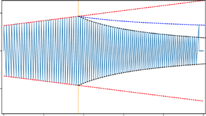
For a final demonstration, we show in figure 4 that the adiabatic invariance of ${\mathcal {R}}_\pm$ can be used to adapt Whitham's equal-area method to weak shock evolution within a varying background. Here, a wave train is introduced for which the initial waveform is a ‘reverse sawtooth’ with a linear rise and sudden decline in ${\mathcal {R}}_+(t_0)$. The waveform converts to a ‘forward sawtooth’ at the point of shock formation. After shock formation, the wave dissipates in a manner we discuss in detail in a companion paper (Matzner & Ro Reference Matzner and Ro2021). Notably, the leading or ‘head’ shock decays distinctly more slowly than the ‘internal’ shocks that form within the wave train.

Figure 4. One snapshot of shock evolution within a wave with an initial ‘reverse sawtooth’ waveform. The simulation matches analytical predictions for the shock formation radius (orange vertical line) and for the velocity amplitudes of the head shock and internal shocks (blue and black dashed lines, respectively) to high accuracy. These predictions, discussed in depth in a companion paper (Matzner & Ro Reference Matzner and Ro2021), rely on the adiabatic invariance of ${\mathcal {R}}_+$.

8. Summary and conclusions

Our primary findings are as follows:

1. (i) The linearized equations of hydrodynamics are compactly expressed (5.4) in terms of wave amplitudes ${\mathcal {R}}_\pm$, which interact in the presence of variations of the impedance.

2. (ii) In the context of ‘quasi-simple’ waves (§ 5.1) – those in which one wave family is absent and not regenerated by reflection – the conservation of ${\mathcal {R}}_+$ or ${\mathcal {R}}_-$ is consistent with the invariant proposed by Lighthill (Reference Lighthill1978), and also with the conservation of wave luminosity (§ 5.2).

3. (iii) Familiar results about the dynamics of reflection follow directly from the amplitude equation (§5.3). In particular, wave reflection is strongly suppressed in the high-frequency limit.

4. (iv) Lighthill's proposition amounts to the statement that linear conservation laws may be extrapolated into the mildly nonlinear regime, providing a simple means to calculate wave self-distortion and shock formation, as well as weak shock dissipation by Whitham's equal-area method. We validate this method and delimit its validity. In the high-frequency limit, the nonlinear error is minimal at the point of shock formation (§ 6.2). Because there is no nonlinear error at the wave node, Lighthill's criterion for shock formation is exact so long as the shock forms at a node and reflection is negligible, as it is for ‘head’ shocks, and for any shocks generated within high-frequency waves (§ 6.3).

5. (v) Going beyond linearized theory, we find that nonlinear solutions are available in a restricted class of problems (§ 6.1). In the example considered, the novel element is a nonlinear correction to the wave amplitude, which leads to a modified phase speed.

In a companion work (Matzner & Ro Reference Matzner and Ro2021), we use these findings to predict the evolution of shock strength and shock dissipation in the context of super-Eddington outbursts of evolved massive stars. There, we provide useful formulae for the shock-deposited heat, and we evaluate the potential of head shocks to eject matter from the stellar surface.