


1 Introduction
Superhydrophobic (SH) surfaces have received much attention as a means of skin-friction drag reduction in wall-bounded turbulent flows in recent years (Rothstein Reference Rothstein2010). These are surfaces with apparent receding contact angle exceeding a certain value, e.g.
 $150^{\circ }$
(Schellenberger et al.
Reference Schellenberger, Encinas, Vollmer and Butt2016), which repel liquids by trapping gas inside the nano- or micro-scale features of a textured hydrophobic surface. The entrapped gas prevents direct contact between the liquid and the wall, leading to the so-called Cassie–Baxter state, and providing a mechanism for liquid slip at the wall. This effective slip has been shown to be the primary mechanism of skin-friction drag reduction with SH surfaces in both the laminar and turbulent flow regimes (Rastegari & Akhavan Reference Rastegari and Akhavan2015, Reference Rastegari and Akhavan2018a
).
$150^{\circ }$
(Schellenberger et al.
Reference Schellenberger, Encinas, Vollmer and Butt2016), which repel liquids by trapping gas inside the nano- or micro-scale features of a textured hydrophobic surface. The entrapped gas prevents direct contact between the liquid and the wall, leading to the so-called Cassie–Baxter state, and providing a mechanism for liquid slip at the wall. This effective slip has been shown to be the primary mechanism of skin-friction drag reduction with SH surfaces in both the laminar and turbulent flow regimes (Rastegari & Akhavan Reference Rastegari and Akhavan2015, Reference Rastegari and Akhavan2018a
).
Drag reductions of up to 50 % (Daniello, Waterhouse & Rothstein Reference Daniello, Waterhouse and Rothstein2009) and up to 75 % (Park, Sun & Kim Reference Park, Sun and Kim2014) have been reported in laboratory-scale experiments in turbulent channel flows and turbulent boundary layer flows, at
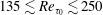 $135\lesssim Re_{\unicode[STIX]{x1D70F}_{0}}\lesssim 250$
, using SH longitudinal microgrooves with solid fractions of
$135\lesssim Re_{\unicode[STIX]{x1D70F}_{0}}\lesssim 250$
, using SH longitudinal microgrooves with solid fractions of
 $\unicode[STIX]{x1D719}_{s}=0.5$
and
$\unicode[STIX]{x1D719}_{s}=0.5$
and
 $\unicode[STIX]{x1D719}_{s}=0.05$
, respectively, where
$\unicode[STIX]{x1D719}_{s}=0.05$
, respectively, where
 $Re_{\unicode[STIX]{x1D70F}_{0}}\equiv u_{\unicode[STIX]{x1D70F}_{0}}\unicode[STIX]{x1D6FF}/\unicode[STIX]{x1D708}$
is the friction Reynolds number in the base flow,
$Re_{\unicode[STIX]{x1D70F}_{0}}\equiv u_{\unicode[STIX]{x1D70F}_{0}}\unicode[STIX]{x1D6FF}/\unicode[STIX]{x1D708}$
is the friction Reynolds number in the base flow,
 $u_{\unicode[STIX]{x1D70F}_{0}}$
is the wall friction velocity in the base flow,
$u_{\unicode[STIX]{x1D70F}_{0}}$
is the wall friction velocity in the base flow,
 $\unicode[STIX]{x1D6FF}$
is the boundary layer thickness or channel half-height and
$\unicode[STIX]{x1D6FF}$
is the boundary layer thickness or channel half-height and
 $\unicode[STIX]{x1D708}$
is the kinematic viscosity. It has been noted that the magnitude of drag reduction increases with increasing width of the surface microtexture indentations,
$\unicode[STIX]{x1D708}$
is the kinematic viscosity. It has been noted that the magnitude of drag reduction increases with increasing width of the surface microtexture indentations,
 $g$
, and decreasing solid fraction,
$g$
, and decreasing solid fraction,
 $\unicode[STIX]{x1D719}_{s}$
, approaching a maximum drag reduction of
$\unicode[STIX]{x1D719}_{s}$
, approaching a maximum drag reduction of
 $DR\sim (1-\unicode[STIX]{x1D719}_{s})$
in the limit of large
$DR\sim (1-\unicode[STIX]{x1D719}_{s})$
in the limit of large
 $g$
(Daniello et al.
Reference Daniello, Waterhouse and Rothstein2009; Rothstein Reference Rothstein2010; Park, Park & Kim Reference Park, Park and Kim2013). Scaling laws have been proposed for the slip length and the slip velocity in terms of
$g$
(Daniello et al.
Reference Daniello, Waterhouse and Rothstein2009; Rothstein Reference Rothstein2010; Park, Park & Kim Reference Park, Park and Kim2013). Scaling laws have been proposed for the slip length and the slip velocity in terms of
 $g$
and
$g$
and
 $\unicode[STIX]{x1D719}_{s}$
in both the laminar (Ybert et al.
Reference Ybert, Barentin, Cottin-Bizonne, Joseph and Bocquet2007) and turbulent (Seo & Mani Reference Seo and Mani2016) flow regimes. However, the relation between these scaling laws and the magnitude of drag reduction has not been clarified.
$\unicode[STIX]{x1D719}_{s}$
in both the laminar (Ybert et al.
Reference Ybert, Barentin, Cottin-Bizonne, Joseph and Bocquet2007) and turbulent (Seo & Mani Reference Seo and Mani2016) flow regimes. However, the relation between these scaling laws and the magnitude of drag reduction has not been clarified.
These drag reduction capabilities of SH surfaces, however, are lost if the SH surface undergoes a wetting transition, from the Cassie–Baxter state to a Wenzel state, whereby the trapped gas pockets inside the surface microtexture are depleted and replaced with the working fluid. This wetting transition can occur because of (i) depinning of the contact line and/or sagging of the liquid–gas interface under high local pressures (Zheng, Yu & Zhao Reference Zheng, Yu and Zhao2005; Checco et al. Reference Checco, Ocko, Rahman, Black, Tasinkevych, Giacomello and Dietrich2014) or (ii) diffusion or entrainment of the gas layer into the working liquid under high local shear rates (Samaha, Tafreshi & Gad-el Hak Reference Samaha, Tafreshi and Gad-el Hak2012; Karatay, Tsai & Lammertink Reference Karatay, Tsai and Lammertink2013; Wexler, Jacobi & Stone Reference Wexler, Jacobi and Stone2015; Ling et al. Reference Ling, Katz, Fu and Hultmark2017) of turbulent flow.
There is also anecdotal evidence, from both direct numerical simulation (DNS) and experiments, which suggests that, for a given geometry and size of the surface microtexture in wall units, the drag reduction performance of SH surfaces degrades with increasing Reynolds number of the base flow (Rastegari & Akhavan Reference Rastegari and Akhavan2018a
). Here, and throughout this study, ‘wall units’ refers to normalization with respect to the wall friction velocity of the drag reduced flow,
 $u_{\unicode[STIX]{x1D70F}}$
, and the kinematic viscosity,
$u_{\unicode[STIX]{x1D70F}}$
, and the kinematic viscosity,
 $\unicode[STIX]{x1D708}$
, and quantities normalized in this manner are denoted by a
$\unicode[STIX]{x1D708}$
, and quantities normalized in this manner are denoted by a
 $+$
superscript. This degradation in drag reduction has been recently demonstrated in DNS studies of turbulent channel flows with SH longitudinal microgrooves at
$+$
superscript. This degradation in drag reduction has been recently demonstrated in DNS studies of turbulent channel flows with SH longitudinal microgrooves at
 $Re_{\unicode[STIX]{x1D70F}_{0}}\approx 222$
and
$Re_{\unicode[STIX]{x1D70F}_{0}}\approx 222$
and
 $442$
(Rastegari & Akhavan Reference Rastegari and Akhavan2018a
), and can also be observed in earlier DNS studies of turbulent channel flows with SH longitudinal microgrooves at
$442$
(Rastegari & Akhavan Reference Rastegari and Akhavan2018a
), and can also be observed in earlier DNS studies of turbulent channel flows with SH longitudinal microgrooves at
 $180\lesssim Re_{\unicode[STIX]{x1D70F}_{0}}\lesssim 590$
(Park et al.
Reference Park, Park and Kim2013, figure 8b), even though the authors do not comment on it. Evidence of this degradation in drag reduction can also be found in recent experimental studies in turbulent boundary layer flows with spray coated SH walls, where a given upwards shift of the logarithmic layer in wall units, corresponding to
$180\lesssim Re_{\unicode[STIX]{x1D70F}_{0}}\lesssim 590$
(Park et al.
Reference Park, Park and Kim2013, figure 8b), even though the authors do not comment on it. Evidence of this degradation in drag reduction can also be found in recent experimental studies in turbulent boundary layer flows with spray coated SH walls, where a given upwards shift of the logarithmic layer in wall units, corresponding to
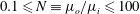
 $\unicode[STIX]{x0394}U^{+}=1.1$
, was found to result in 12 % drag reduction at
$\unicode[STIX]{x0394}U^{+}=1.1$
, was found to result in 12 % drag reduction at
 $Re_{\unicode[STIX]{x1D70F}_{0}}\approx 863$
, but only 11 % drag reduction at
$Re_{\unicode[STIX]{x1D70F}_{0}}\approx 863$
, but only 11 % drag reduction at
 $Re_{\unicode[STIX]{x1D70F}_{0}}\approx 1408$
(Ling et al.
Reference Ling, Srinivasan, Golovin, McKinley, Tuteja and Katz2016).
$Re_{\unicode[STIX]{x1D70F}_{0}}\approx 1408$
(Ling et al.
Reference Ling, Srinivasan, Golovin, McKinley, Tuteja and Katz2016).
While other experimental studies have reported an enhancement of drag reduction with increasing Reynolds number in SH turbulent boundary layer flows (Zhang et al.
Reference Zhang, Tian, Yao, Hao and Jiang2015) or in SH or liquid-infused (LI) turbulent Taylor–Couette flows (Srinivasan et al.
Reference Srinivasan, Kleingartner, Gilbert, Cohen, Milne and McKinley2015; Van Buren & Smits Reference Van Buren and Smits2017), it should be noted that these experiments were not performed with a fixed size of the surface microtexture in wall units at different Reynolds numbers. Instead, they used a given surface microtexture with a fixed size in ‘physical units’ at different Reynolds numbers, which leads to an increase in the size of the surface microtexture in wall units as the Reynolds number increases. As will be discussed in detail in §§ 3 and 4, an increase in the size of the surface microtexture in wall units can affect the drag reduction in a number of conflicting and competing ways. In the absence of a wetting transition or roughness effects, an increase in the size of the surface microtexture in wall units enhances the magnitude of drag reduction. However, an increase in the size of the surface microtexture in wall units also makes the surface more susceptible to a wetting transition, at which point the surface microtexture can begin to act as surface roughness and cause a drag increase. In addition, for random surface microtextures, where the height of the surface micro-features is variable, the protrusion heights of the surface elements above the liquid/gas interface will increase in wall units as the Reynolds number increases. This can also give rise to roughness effects with increasing Reynolds number, which can degrade the drag reduction. The interplay between these competing effects determines the trends in drag reduction when a surface microtexture of a given size in physical units is employed at different Reynolds numbers. Depending on which features are at play or dominate, the magnitude of drag reduction can be enhanced with increasing Reynolds number (Srinivasan et al.
Reference Srinivasan, Kleingartner, Gilbert, Cohen, Milne and McKinley2015; Zhang et al.
Reference Zhang, Tian, Yao, Hao and Jiang2015; Van Buren & Smits Reference Van Buren and Smits2017), or degrade (Bidkar et al.
Reference Bidkar, Leblanc, Kulkarni, Bahadur, Ceccio and Perlin2014; Ling et al.
Reference Ling, Srinivasan, Golovin, McKinley, Tuteja and Katz2016; Reholon & Ghaemi Reference Reholon and Ghaemi2018), or show enhancement at low Reynolds numbers followed by degradation at higher Reynolds numbers (Aljallis et al.
Reference Aljallis, Sarshar, Datla, Sikka, Jones and Choi2013; Bidkar et al.
Reference Bidkar, Leblanc, Kulkarni, Bahadur, Ceccio and Perlin2014; Gose et al.
Reference Gose, Golovin, Boban, Mabry, Tuteja, Perlin and Ceccio2018). Collectively, the available experimental data in high Reynolds number SH turbulent boundary layer flows or SH turbulent channel flows, performed with a fixed size of the surface microtexture in physical units, show a trend towards enhancement of drag reduction with increasing Reynolds number up to a maximum of
 ${\sim}30\,\%$
drag reduction at
${\sim}30\,\%$
drag reduction at
 $Re_{\unicode[STIX]{x1D70F}_{0}}\approx 1500$
(Aljallis et al.
Reference Aljallis, Sarshar, Datla, Sikka, Jones and Choi2013; Zhang et al.
Reference Zhang, Tian, Yao, Hao and Jiang2015; Ling et al.
Reference Ling, Srinivasan, Golovin, McKinley, Tuteja and Katz2016), followed by degradation of drag reduction at higher Reynolds numbers, approaching negative drag reductions at
$Re_{\unicode[STIX]{x1D70F}_{0}}\approx 1500$
(Aljallis et al.
Reference Aljallis, Sarshar, Datla, Sikka, Jones and Choi2013; Zhang et al.
Reference Zhang, Tian, Yao, Hao and Jiang2015; Ling et al.
Reference Ling, Srinivasan, Golovin, McKinley, Tuteja and Katz2016), followed by degradation of drag reduction at higher Reynolds numbers, approaching negative drag reductions at
 $Re_{\unicode[STIX]{x1D70F}_{0}}\gtrsim 5000$
(Aljallis et al.
Reference Aljallis, Sarshar, Datla, Sikka, Jones and Choi2013; Ling et al.
Reference Ling, Srinivasan, Golovin, McKinley, Tuteja and Katz2016). These results all point to the need for an understanding of the scaling of drag reduction and the sustainability bounds of SH and LI surfaces with surface microtexture and flow parameters in turbulent flow.
$Re_{\unicode[STIX]{x1D70F}_{0}}\gtrsim 5000$
(Aljallis et al.
Reference Aljallis, Sarshar, Datla, Sikka, Jones and Choi2013; Ling et al.
Reference Ling, Srinivasan, Golovin, McKinley, Tuteja and Katz2016). These results all point to the need for an understanding of the scaling of drag reduction and the sustainability bounds of SH and LI surfaces with surface microtexture and flow parameters in turbulent flow.
The degradation in the drag reduction performance of microtextured surfaces with increasing Reynolds number of the base flow, for a fixed geometry and size of the surface microtexture in wall units, is a well-known feature of riblets (Bechert et al.
Reference Bechert, Bruse, Hage, Van Der Hoeven and Hoppe1997; Spalart & McLean Reference Spalart and McLean2011), where the highest drag reductions achieved in high Reynolds number turbulent flows of practical interest, with optimal ‘blade riblets’ of spacing
 ${\sim}15$
wall units (Bechert et al.
Reference Bechert, Bruse, Hage, Van Der Hoeven and Hoppe1997), were found to be nearly half the highest drag reductions, of
${\sim}15$
wall units (Bechert et al.
Reference Bechert, Bruse, Hage, Van Der Hoeven and Hoppe1997), were found to be nearly half the highest drag reductions, of
 ${\sim}10\,\%$
, obtained with the same geometry and size of the riblets in wall units in laboratory-scale experiments (Spalart & McLean Reference Spalart and McLean2011). It has been suggested (Bechert et al.
Reference Bechert, Bruse, Hage, Van Der Hoeven and Hoppe1997; Spalart & McLean Reference Spalart and McLean2011; García-Mayoral & Jiménez Reference García-Mayoral and Jiménez2012) that a Reynolds number independent measure of drag reduction can be constructed by parameterizing the magnitude of drag reduction in terms of the friction coefficient of the base flow,
${\sim}10\,\%$
, obtained with the same geometry and size of the riblets in wall units in laboratory-scale experiments (Spalart & McLean Reference Spalart and McLean2011). It has been suggested (Bechert et al.
Reference Bechert, Bruse, Hage, Van Der Hoeven and Hoppe1997; Spalart & McLean Reference Spalart and McLean2011; García-Mayoral & Jiménez Reference García-Mayoral and Jiménez2012) that a Reynolds number independent measure of drag reduction can be constructed by parameterizing the magnitude of drag reduction in terms of the friction coefficient of the base flow,
 $C_{f_{0}}$
, and the shift,
$C_{f_{0}}$
, and the shift,
 $(B-B_{0})$
, in the intercepts,
$(B-B_{0})$
, in the intercepts,
 $B$
and
$B$
and
 $B_{0}$
, of log-law representations of the normalized mean velocity profiles in the drag reduced and the base flow, respectively, where
$B_{0}$
, of log-law representations of the normalized mean velocity profiles in the drag reduced and the base flow, respectively, where
 $(B-B_{0})$
is Reynolds number independent and only a function of the geometry and size of the surface microtexture in wall units. In Rastegari & Akhavan (Reference Rastegari and Akhavan2018a
), this formulation was extended to SH surfaces to obtain a parameterization of the magnitude of SH drag reduction in terms of
$(B-B_{0})$
is Reynolds number independent and only a function of the geometry and size of the surface microtexture in wall units. In Rastegari & Akhavan (Reference Rastegari and Akhavan2018a
), this formulation was extended to SH surfaces to obtain a parameterization of the magnitude of SH drag reduction in terms of
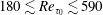
 $C_{f_{0}}$
and the shift
$C_{f_{0}}$
and the shift
 $(B-B_{0})$
.
$(B-B_{0})$
.
While such a parametrization allows the drag reduction results from low Reynolds number turbulent flows to be extrapolated to higher Reynolds number flows of practical interest (Rastegari & Akhavan Reference Rastegari and Akhavan2018a
), developing optimal designs of SH surfaces also requires an understanding of the scaling laws for
 $(B-B_{0})$
in terms of the geometrical parameters of the surface microtexture, as well as the sustainability bounds of SH surfaces in turbulent flow.
$(B-B_{0})$
in terms of the geometrical parameters of the surface microtexture, as well as the sustainability bounds of SH surfaces in turbulent flow.
In this study, scaling arguments are combined with results from DNS of SH turbulent channel flows at
 $Re_{\unicode[STIX]{x1D70F}_{0}}\approx 222$
and
$Re_{\unicode[STIX]{x1D70F}_{0}}\approx 222$
and
 $442$
, performed with a wide range of SH longitudinal microgroove or aligned micropost surface microtexture geometrical parameters, to demonstrate the Reynolds number dependence of the drag reduction, and the Reynolds number independence of
$442$
, performed with a wide range of SH longitudinal microgroove or aligned micropost surface microtexture geometrical parameters, to demonstrate the Reynolds number dependence of the drag reduction, and the Reynolds number independence of
 $(B-B_{0})$
, and to present the scaling laws for
$(B-B_{0})$
, and to present the scaling laws for
 $(B-B_{0})$
in turbulent flow in terms of the geometrical parameters of the SH surface in wall units. The combination of these parametrizations allow for a priori prediction of the magnitude of drag reduction with SH surfaces in turbulent flow at any Reynolds number. For the most stable of such SH surfaces, namely longitudinal microgrooves, we further present the pressure stability bounds of the SH surface in turbulent flow in terms of the Weber number, the geometrical parameters of the SH surface in wall units and the friction Reynolds number of the flow. These parameterizations are used to identify the narrow range of SH surface geometrical parameters which can ensure large drag reduction as well as sustainability in high Reynolds number turbulent flows of practical interest.
$(B-B_{0})$
in turbulent flow in terms of the geometrical parameters of the SH surface in wall units. The combination of these parametrizations allow for a priori prediction of the magnitude of drag reduction with SH surfaces in turbulent flow at any Reynolds number. For the most stable of such SH surfaces, namely longitudinal microgrooves, we further present the pressure stability bounds of the SH surface in turbulent flow in terms of the Weber number, the geometrical parameters of the SH surface in wall units and the friction Reynolds number of the flow. These parameterizations are used to identify the narrow range of SH surface geometrical parameters which can ensure large drag reduction as well as sustainability in high Reynolds number turbulent flows of practical interest.
2 Numerical methods and simulation parameters
The DNS studies were performed in turbulent channel flows using standard D3Q19 (three-dimensional, 19 discrete velocity), single-relaxation-time lattice Boltzmann methods (Succi Reference Succi2001) with grid embedding (Lagrava et al.
Reference Lagrava, Malaspinas, Latt and Chopard2012), of grid ratio
 $4:1$
, in the near-wall regions to better resolve the flow features near the SH walls. The resulting grid spacings were
$4:1$
, in the near-wall regions to better resolve the flow features near the SH walls. The resulting grid spacings were
 $\unicode[STIX]{x1D6E5}_{f}^{+0}\approx 0.5$
for
$\unicode[STIX]{x1D6E5}_{f}^{+0}\approx 0.5$
for
 $z^{+0}\lesssim 30$
, and
$z^{+0}\lesssim 30$
, and
 $\unicode[STIX]{x1D6E5}_{c}^{+0}\approx 2$
for
$\unicode[STIX]{x1D6E5}_{c}^{+0}\approx 2$
for
 $z^{+0}\gtrsim 30$
in all three directions in all the simulations, where
$z^{+0}\gtrsim 30$
in all three directions in all the simulations, where
 $\unicode[STIX]{x1D6E5}_{f}$
and
$\unicode[STIX]{x1D6E5}_{f}$
and
 $\unicode[STIX]{x1D6E5}_{c}$
denote the grid spacings on the fine grid and the coarse grid, respectively, and the
$\unicode[STIX]{x1D6E5}_{c}$
denote the grid spacings on the fine grid and the coarse grid, respectively, and the
 $+0$
superscript denotes normalization with respect to the kinematic viscosity,
$+0$
superscript denotes normalization with respect to the kinematic viscosity,
 $\unicode[STIX]{x1D708}$
, and the wall-friction velocity,
$\unicode[STIX]{x1D708}$
, and the wall-friction velocity,
 $u_{\unicode[STIX]{x1D70F}_{0}}$
, of a ‘base’ turbulent channel flow with smooth, no-slip walls at the same bulk Reynolds number as the channel flow with SH walls. To preserve the order of accuracy of the lattice Boltzmann method, and ensure smoothness and continuity of the variables at the transition between the coarse and the fine grids, the two grids were overlapped for one cell width of the coarse grid, as suggested by Lagrava et al. (Reference Lagrava, Malaspinas, Latt and Chopard2012), and the interpolations between the two grids were performed using third-order bi-cubic Hermite splines in space, and second-order Hermite polynomials in time. The details of the numerical methods and verification studies performed to ensure the accuracy of the numerical methods and adequacy of the domain sizes and grid resolutions are described in the appendix of Rastegari & Akhavan (Reference Rastegari and Akhavan2018a
).
$u_{\unicode[STIX]{x1D70F}_{0}}$
, of a ‘base’ turbulent channel flow with smooth, no-slip walls at the same bulk Reynolds number as the channel flow with SH walls. To preserve the order of accuracy of the lattice Boltzmann method, and ensure smoothness and continuity of the variables at the transition between the coarse and the fine grids, the two grids were overlapped for one cell width of the coarse grid, as suggested by Lagrava et al. (Reference Lagrava, Malaspinas, Latt and Chopard2012), and the interpolations between the two grids were performed using third-order bi-cubic Hermite splines in space, and second-order Hermite polynomials in time. The details of the numerical methods and verification studies performed to ensure the accuracy of the numerical methods and adequacy of the domain sizes and grid resolutions are described in the appendix of Rastegari & Akhavan (Reference Rastegari and Akhavan2018a
).
The liquid/gas interfaces on SH walls were modelled as stationary, curved or flat shear-free boundaries, with the shape of the meniscus determined from an analytical solution of the Young–Laplace equation (Rastegari & Akhavan Reference Rastegari and Akhavan2018a
). Two interface protrusion angles of
 $\unicode[STIX]{x1D703}_{p}=0^{\circ }$
and
$\unicode[STIX]{x1D703}_{p}=0^{\circ }$
and
 $\unicode[STIX]{x1D703}_{p}=-30^{\circ }$
were investigated, corresponding to liquid/gas interfaces which were either flat or at maximum advancing contact angle (
$\unicode[STIX]{x1D703}_{p}=-30^{\circ }$
were investigated, corresponding to liquid/gas interfaces which were either flat or at maximum advancing contact angle (
 $\unicode[STIX]{x1D703}_{c}=\unicode[STIX]{x1D703}_{F,adv}=120^{\circ }$
), respectively.
$\unicode[STIX]{x1D703}_{c}=\unicode[STIX]{x1D703}_{F,adv}=120^{\circ }$
), respectively.
The simulations were performed in channels of size
 $5h\times 2.5h\times 2h$
in the streamwise (
$5h\times 2.5h\times 2h$
in the streamwise (
 $x$
), spanwise (
$x$
), spanwise (
 $y$
) and wall-normal (
$y$
) and wall-normal (
 $z$
) directions, respectively, as shown in figure 1. A constant flow rate was maintained in the channel during the course of all simulations, corresponding to bulk Reynolds numbers of
$z$
) directions, respectively, as shown in figure 1. A constant flow rate was maintained in the channel during the course of all simulations, corresponding to bulk Reynolds numbers of
 $Re_{b}\equiv q/2\unicode[STIX]{x1D708}=3600$
or
$Re_{b}\equiv q/2\unicode[STIX]{x1D708}=3600$
or
 $Re_{b}=7860$
, where
$Re_{b}=7860$
, where
 $q$
denotes the flow rate per unit spanwise width in the channel. For reference, DNS studies were also performed in base turbulent channel flows with smooth, no-slip walls at the same
$q$
denotes the flow rate per unit spanwise width in the channel. For reference, DNS studies were also performed in base turbulent channel flows with smooth, no-slip walls at the same
 $Re_{b}$
as the SH channels. The corresponding friction Reynolds numbers in the base turbulent channel flows were
$Re_{b}$
as the SH channels. The corresponding friction Reynolds numbers in the base turbulent channel flows were
 $Re_{\unicode[STIX]{x1D70F}_{0}}\equiv u_{\unicode[STIX]{x1D70F}_{0}}h/\unicode[STIX]{x1D708}\approx 222$
at
$Re_{\unicode[STIX]{x1D70F}_{0}}\equiv u_{\unicode[STIX]{x1D70F}_{0}}h/\unicode[STIX]{x1D708}\approx 222$
at
 $Re_{b}=3600$
, and
$Re_{b}=3600$
, and
 $Re_{\unicode[STIX]{x1D70F}_{0}}\approx 442$
at
$Re_{\unicode[STIX]{x1D70F}_{0}}\approx 442$
at
 $Re_{b}=7860$
.
$Re_{b}=7860$
.

Figure 1. Schematic of the channels with SH walls, the coordinate system and the computational grid: (a) SH longitudinal microgrooves; (b) SH aligned microposts; (c) computational grid and protrusion angle.
A total of 53 simulations were performed with SH longitudinal microgrooves, covering the range of microgroove widths
 $4\lesssim g^{+0}\lesssim 128$
, solid fractions of
$4\lesssim g^{+0}\lesssim 128$
, solid fractions of
 $1/64\leqslant \unicode[STIX]{x1D719}_{s}\leqslant 1/2$
, protrusion angles of
$1/64\leqslant \unicode[STIX]{x1D719}_{s}\leqslant 1/2$
, protrusion angles of
 $\unicode[STIX]{x1D703}_{p}=0^{\circ }$
and
$\unicode[STIX]{x1D703}_{p}=0^{\circ }$
and
 $\unicode[STIX]{x1D703}_{p}=-30^{\circ }$
and bulk Reynolds numbers of
$\unicode[STIX]{x1D703}_{p}=-30^{\circ }$
and bulk Reynolds numbers of
 $Re_{b}=3600$
(
$Re_{b}=3600$
(
 $Re_{\unicode[STIX]{x1D70F}_{0}}\approx 222$
) and
$Re_{\unicode[STIX]{x1D70F}_{0}}\approx 222$
) and
 $Re_{b}=7860$
(
$Re_{b}=7860$
(
 $Re_{\unicode[STIX]{x1D70F}_{0}}\approx 442$
), as shown in table 1. In addition, as shown in table 1, four simulations were also performed with SH aligned square microposts with
$Re_{\unicode[STIX]{x1D70F}_{0}}\approx 442$
), as shown in table 1. In addition, as shown in table 1, four simulations were also performed with SH aligned square microposts with
 $g^{+0}\approx 28,56$
,
$g^{+0}\approx 28,56$
,
 $\unicode[STIX]{x1D719}_{s}=1/64$
and
$\unicode[STIX]{x1D719}_{s}=1/64$
and
 $\unicode[STIX]{x1D703}_{p}=0^{\circ }$
at
$\unicode[STIX]{x1D703}_{p}=0^{\circ }$
at
 $Re_{b}=3600$
(
$Re_{b}=3600$
(
 $Re_{\unicode[STIX]{x1D70F}_{0}}\approx 222$
) and
$Re_{\unicode[STIX]{x1D70F}_{0}}\approx 222$
) and
 $Re_{b}=7860$
(
$Re_{b}=7860$
(
 $Re_{\unicode[STIX]{x1D70F}_{0}}\approx 442$
).
$Re_{\unicode[STIX]{x1D70F}_{0}}\approx 442$
).
Table 1. Summary of simulation parameters and resulting drag reductions,
 $DR$
, in the present study.
$DR$
, in the present study.

3 The scaling of drag reduction with surface microtexture and flow parameters
It has been suggested that in drag reduction with microtextured surfaces, be they riblets, SH surfaces or liquid-infused (LI) surfaces, the magnitude of drag reduction depends not only on the geometry and size of the surface microtexture in wall units, but also the Reynolds number of the base flow (Bechert et al.
Reference Bechert, Bruse, Hage, Van Der Hoeven and Hoppe1997; Spalart & McLean Reference Spalart and McLean2011; García-Mayoral & Jiménez Reference García-Mayoral and Jiménez2012; Rastegari & Akhavan Reference Rastegari and Akhavan2018a
). It has also been suggested (Bechert et al.
Reference Bechert, Bruse, Hage, Van Der Hoeven and Hoppe1997; Spalart & McLean Reference Spalart and McLean2011) that a Reynolds number independent measure of drag reduction can be constructed by representing the normalized mean velocity profiles in the base flow and in the flow with microtextured walls as logarithmic profiles,
 $\langle \overline{U}\rangle /u_{\unicode[STIX]{x1D70F}_{0}}=(1/\unicode[STIX]{x1D705})\ln z^{+0}+B_{0}$
and
$\langle \overline{U}\rangle /u_{\unicode[STIX]{x1D70F}_{0}}=(1/\unicode[STIX]{x1D705})\ln z^{+0}+B_{0}$
and
 $\langle \overline{U}\rangle /u_{\unicode[STIX]{x1D70F}}=(1/\unicode[STIX]{x1D705})\ln z^{+}+B$
, throughout the cross-section of the flow, and expressing the magnitude of drag reduction in terms of the shift,
$\langle \overline{U}\rangle /u_{\unicode[STIX]{x1D70F}}=(1/\unicode[STIX]{x1D705})\ln z^{+}+B$
, throughout the cross-section of the flow, and expressing the magnitude of drag reduction in terms of the shift,
 $(B-B_{0})$
, in the intercepts of these logarithmic-law representations of the mean velocity profiles, as shown in the figure 2. Here, and throughout this study, an overbar denotes Reynolds averaging in time and any homogeneous flow directions, and brackets
$(B-B_{0})$
, in the intercepts of these logarithmic-law representations of the mean velocity profiles, as shown in the figure 2. Here, and throughout this study, an overbar denotes Reynolds averaging in time and any homogeneous flow directions, and brackets
 $\langle \,\rangle$
denote averaging in the wall-parallel directions.
$\langle \,\rangle$
denote averaging in the wall-parallel directions.
Using this formulation, the magnitude of drag reduction with microtextured surfaces can be expressed as (Rastegari & Akhavan Reference Rastegari and Akhavan2018a )
 $$\begin{eqnarray}\left(1-DR\right)=\left\{1+\left[\frac{1}{2\unicode[STIX]{x1D705}}\ln (1-DR)+(B-B_{0})\right]\sqrt{\frac{C_{f_{0}}}{2}}\right\}^{-2},\end{eqnarray}$$
where
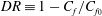 $DR\equiv 1-C_{f}/C_{f_{0}}$
is the magnitude of drag reduction,
$DR\equiv 1-C_{f}/C_{f_{0}}$
is the magnitude of drag reduction,
 $C_{f}$
and
$C_{f}$
and
 $C_{f_{0}}$
are the skin-friction coefficients in the flow with microtextured walls and in the base flow with smooth no-slip walls, defined as
$C_{f_{0}}$
are the skin-friction coefficients in the flow with microtextured walls and in the base flow with smooth no-slip walls, defined as
 $C_{f}\equiv 2u_{\unicode[STIX]{x1D70F}}^{2}/U_{b}^{2}$
and
$C_{f}\equiv 2u_{\unicode[STIX]{x1D70F}}^{2}/U_{b}^{2}$
and
 $C_{f_{0}}\equiv 2u_{\unicode[STIX]{x1D70F}_{0}}^{2}/U_{b_{0}}^{2}$
in internal flow and
$C_{f_{0}}\equiv 2u_{\unicode[STIX]{x1D70F}_{0}}^{2}/U_{b_{0}}^{2}$
in internal flow and
 $C_{f}\equiv 2u_{\unicode[STIX]{x1D70F}}^{2}/U_{\infty }^{2}$
and
$C_{f}\equiv 2u_{\unicode[STIX]{x1D70F}}^{2}/U_{\infty }^{2}$
and
 $C_{f_{0}}\equiv 2u_{\unicode[STIX]{x1D70F}_{0}}^{2}/U_{\infty }^{2}$
in external flow, respectively,
$C_{f_{0}}\equiv 2u_{\unicode[STIX]{x1D70F}_{0}}^{2}/U_{\infty }^{2}$
in external flow, respectively,
 $\unicode[STIX]{x1D705}$
is the von Kármán constant, and
$\unicode[STIX]{x1D705}$
is the von Kármán constant, and
 $(B-B_{0})$
is Reynolds number independent and only a function of the geometry and size of the surface microtexture in wall units. The appearance of
$(B-B_{0})$
is Reynolds number independent and only a function of the geometry and size of the surface microtexture in wall units. The appearance of
 $C_{f_{0}}$
in (3.1) leads to a degradation in the magnitude of drag reduction with increasing Reynolds number of the base flow for a given
$C_{f_{0}}$
in (3.1) leads to a degradation in the magnitude of drag reduction with increasing Reynolds number of the base flow for a given
 $(B-B_{0})$
.
$(B-B_{0})$
.

Figure 2. Schematic representation of
 $(B-B_{0})$
and
$(B-B_{0})$
and
 $U_{s}^{+}$
in turbulent flow with microtextured walls: —— (black), –
$U_{s}^{+}$
in turbulent flow with microtextured walls: —— (black), –
 $\cdot$
 $\cdot$
– (turquoise), mean velocity profiles in the base turbulent flow and the flow with microtextured walls, respectively; – – – (black), –
$\cdot$
– (turquoise), mean velocity profiles in the base turbulent flow and the flow with microtextured walls, respectively; – – – (black), –
 $\cdot$
– (turquoise), logarithmic representations of the mean velocity profiles in the base turbulent flow and the flow with microtextured walls, respectively.
$\cdot$
– (turquoise), logarithmic representations of the mean velocity profiles in the base turbulent flow and the flow with microtextured walls, respectively.
It was brought to our attention by one of the anonymous referees that (3.1) can be recast into an explicit expression for
 $DR$
, given by
$DR$
, given by
 $$\begin{eqnarray}DR=1-\unicode[STIX]{x1D705}^{2}\left(\frac{2}{C_{f_{0}}}\right)\left\{W\left(\unicode[STIX]{x1D705}\sqrt{\frac{2}{C_{f_{0}}}}\exp \left(\unicode[STIX]{x1D705}\left[(B-B_{0})+\sqrt{\frac{2}{C_{f_{0}}}}\right]\right)\right)\right\}^{-2},\end{eqnarray}$$
where
 $W$
denotes the Lambert
$W$
denotes the Lambert
 $W$
function.
$W$
function.

Figure 3. The magnitude of drag reduction,
 $DR$
, as a function of
$DR$
, as a function of
 $(B-B_{0})$
and the friction Reynolds number of the base flow,
$(B-B_{0})$
and the friction Reynolds number of the base flow,
 $Re_{\unicode[STIX]{x1D70F}_{0}}$
. Present DNS studies in SH turbulent channel flow:
$Re_{\unicode[STIX]{x1D70F}_{0}}$
. Present DNS studies in SH turbulent channel flow:
 $Re_{\unicode[STIX]{x1D70F}_{0}}\approx 222$
,
$Re_{\unicode[STIX]{x1D70F}_{0}}\approx 222$
,
 $\unicode[STIX]{x1D703}_{p}=0^{\circ }$
,
$\unicode[STIX]{x1D703}_{p}=0^{\circ }$
,
 $\unicode[STIX]{x1D719}_{s}=1/2$
,
$\unicode[STIX]{x1D719}_{s}=1/2$
,
 $1/8$
,
$1/8$
,
 $1/16$
,
$1/16$
,
 $1/32$
,
$1/32$
,
 $1/64$
;
$1/64$
;  $Re_{\unicode[STIX]{x1D70F}_{0}}\approx 222$
,
$Re_{\unicode[STIX]{x1D70F}_{0}}\approx 222$
,
 $\unicode[STIX]{x1D703}_{p}=-30^{\circ }$
,
$\unicode[STIX]{x1D703}_{p}=-30^{\circ }$
,
 $\unicode[STIX]{x1D719}_{s}=1/2$
,
$\unicode[STIX]{x1D719}_{s}=1/2$
,
 $1/8$
,
$1/8$
,
 $1/16$
,
$1/16$
,
 $1/32$
,
$1/32$
,
 $1/64$
;
$1/64$
;  $Re_{\unicode[STIX]{x1D70F}_{0}}\approx 442$
,
$Re_{\unicode[STIX]{x1D70F}_{0}}\approx 442$
,
 $\unicode[STIX]{x1D703}_{p}=0^{\circ }$
,
$\unicode[STIX]{x1D703}_{p}=0^{\circ }$
,
 $\unicode[STIX]{x1D719}_{s}=1/8$
,
$\unicode[STIX]{x1D719}_{s}=1/8$
,
 $1/16$
,
$1/16$
,
 $1/32$
,
$1/32$
,
 $1/64$
;
$1/64$
;  $Re_{\unicode[STIX]{x1D70F}_{0}}\approx 442$
,
$Re_{\unicode[STIX]{x1D70F}_{0}}\approx 442$
,
 $\unicode[STIX]{x1D703}_{p}=-30^{\circ }$
,
$\unicode[STIX]{x1D703}_{p}=-30^{\circ }$
,
 $\unicode[STIX]{x1D719}_{s}=1/8$
,
$\unicode[STIX]{x1D719}_{s}=1/8$
,
 $1/16$
,
$1/16$
,
 $1/32$
,
$1/32$
,
 $1/64$
;
$1/64$
;  $Re_{\unicode[STIX]{x1D70F}_{0}}\approx 222$
,
$Re_{\unicode[STIX]{x1D70F}_{0}}\approx 222$
,
 $\unicode[STIX]{x1D703}_{p}=0^{\circ }$
,
$\unicode[STIX]{x1D703}_{p}=0^{\circ }$
,
 $\unicode[STIX]{x1D719}_{s}=1/64$
;
$\unicode[STIX]{x1D719}_{s}=1/64$
;  $Re_{\unicode[STIX]{x1D70F}_{0}}\approx 442$
,
$Re_{\unicode[STIX]{x1D70F}_{0}}\approx 442$
,
 $\unicode[STIX]{x1D703}_{p}=0^{\circ }$
,
$\unicode[STIX]{x1D703}_{p}=0^{\circ }$
,
 $\unicode[STIX]{x1D719}_{s}=1/64$
;
$\unicode[STIX]{x1D719}_{s}=1/64$
;  $Re_{\unicode[STIX]{x1D70F}_{0}}\approx 180$
,
$Re_{\unicode[STIX]{x1D70F}_{0}}\approx 180$
,
 $\unicode[STIX]{x1D703}_{p}=0^{o}$
,
$\unicode[STIX]{x1D703}_{p}=0^{o}$
,
 $\unicode[STIX]{x1D719}_{s}=1/2$
,
$\unicode[STIX]{x1D719}_{s}=1/2$
,
 $N=0.1,1,2.5,10,20,100$
(Fu et al.
Reference Fu, Arenas, Leonardi and Hultmark2017); ▪ (red), experiments in turbulent boundary layer flow with SH random microposts,
$N=0.1,1,2.5,10,20,100$
(Fu et al.
Reference Fu, Arenas, Leonardi and Hultmark2017); ▪ (red), experiments in turbulent boundary layer flow with SH random microposts,
 $Re_{\unicode[STIX]{x1D70F}_{0}}\approx 460$
and
$Re_{\unicode[STIX]{x1D70F}_{0}}\approx 460$
and
 $560$
(Zhang et al.
Reference Zhang, Tian, Yao, Hao and Jiang2015); ♦ (green), experiments in turbulent Taylor–Couette flow with SH random microposts,
$560$
(Zhang et al.
Reference Zhang, Tian, Yao, Hao and Jiang2015); ♦ (green), experiments in turbulent Taylor–Couette flow with SH random microposts,
 $Re_{\unicode[STIX]{x1D70F}_{0}}\approx 1193$
and
$Re_{\unicode[STIX]{x1D70F}_{0}}\approx 1193$
and
 $3810$
(Srinivasan et al.
Reference Srinivasan, Kleingartner, Gilbert, Cohen, Milne and McKinley2015); ● (orange), experiments in turbulent boundary layer flow with SH longitudinal microgrooves or SH random microposts,
$3810$
(Srinivasan et al.
Reference Srinivasan, Kleingartner, Gilbert, Cohen, Milne and McKinley2015); ● (orange), experiments in turbulent boundary layer flow with SH longitudinal microgrooves or SH random microposts,
 $Re_{\unicode[STIX]{x1D70F}_{0}}\approx 863,1408$
and
$Re_{\unicode[STIX]{x1D70F}_{0}}\approx 863,1408$
and
 $4287$
(Ling et al.
Reference Ling, Srinivasan, Golovin, McKinley, Tuteja and Katz2016). The black lines show the predictions of (3.1) in turbulent channel flow for: ——,
$4287$
(Ling et al.
Reference Ling, Srinivasan, Golovin, McKinley, Tuteja and Katz2016). The black lines show the predictions of (3.1) in turbulent channel flow for: ——,
 $Re_{\unicode[STIX]{x1D70F}_{0}}\approx 222$
(
$Re_{\unicode[STIX]{x1D70F}_{0}}\approx 222$
(
 $Re_{b}=3600$
); — —,
$Re_{b}=3600$
); — —,
 $Re_{\unicode[STIX]{x1D70F}_{0}}\approx 442$
(
$Re_{\unicode[STIX]{x1D70F}_{0}}\approx 442$
(
 $Re_{b}=7860$
); – – –,
$Re_{b}=7860$
); – – –,
 $Re_{\unicode[STIX]{x1D70F}_{0}}=10^{3}$
(
$Re_{\unicode[STIX]{x1D70F}_{0}}=10^{3}$
(
 $Re_{b}\approx 2\times 10^{4}$
); –
$Re_{b}\approx 2\times 10^{4}$
); –
 $\cdot$
–,
$\cdot$
–,
 $Re_{\unicode[STIX]{x1D70F}_{0}}=10^{4}$
(
$Re_{\unicode[STIX]{x1D70F}_{0}}=10^{4}$
(
 $Re_{b}\approx 2.6\times 10^{5}$
); –
$Re_{b}\approx 2.6\times 10^{5}$
); –
 $\cdot$
 $\cdot$
–,
$\cdot$
–,
 $Re_{\unicode[STIX]{x1D70F}_{0}}=10^{5}$
(
$Re_{\unicode[STIX]{x1D70F}_{0}}=10^{5}$
(
 $Re_{b}\approx 3.2\times 10^{6}$
);
$Re_{b}\approx 3.2\times 10^{6}$
);
 $\cdots \cdots$
,
$\cdots \cdots$
,
 $Re_{\unicode[STIX]{x1D70F}_{0}}=10^{6}$
(
$Re_{\unicode[STIX]{x1D70F}_{0}}=10^{6}$
(
 $Re_{b}\approx 3.8\times 10^{7}$
).
$Re_{b}\approx 3.8\times 10^{7}$
). Figure 3 shows the predictions of (3.1) in turbulent channel flow for
 $222\lesssim Re_{\unicode[STIX]{x1D70F}_{0}}\lesssim 10^{6}$
compared to results from present DNS studies in turbulent channel flows with SH longitudinal microgrooves or SH aligned microposts at
$222\lesssim Re_{\unicode[STIX]{x1D70F}_{0}}\lesssim 10^{6}$
compared to results from present DNS studies in turbulent channel flows with SH longitudinal microgrooves or SH aligned microposts at
 $Re_{\unicode[STIX]{x1D70F}_{0}}\approx 222$
and
$Re_{\unicode[STIX]{x1D70F}_{0}}\approx 222$
and
 $442$
, as summarized in table 1. For
$442$
, as summarized in table 1. For
 $Re_{\unicode[STIX]{x1D70F}_{0}}\geqslant 1000$
, the values of
$Re_{\unicode[STIX]{x1D70F}_{0}}\geqslant 1000$
, the values of
 $C_{f_{0}}$
in (3.1) were obtained from the logarithmic skin-friction correlation suggested by Zanoun, Nagib & Durst (Reference Zanoun, Nagib and Durst2009), which has been shown to give improved agreement with experimental data at high Reynolds numbers compared to the classical Dean’s correlation (Dean Reference Dean1978). In agreement with the predictions of (3.1), for a given value of
$C_{f_{0}}$
in (3.1) were obtained from the logarithmic skin-friction correlation suggested by Zanoun, Nagib & Durst (Reference Zanoun, Nagib and Durst2009), which has been shown to give improved agreement with experimental data at high Reynolds numbers compared to the classical Dean’s correlation (Dean Reference Dean1978). In agreement with the predictions of (3.1), for a given value of
 $(B-B_{0})$
, the DNS data show small degradations of
$(B-B_{0})$
, the DNS data show small degradations of
 ${\approx}1.0{-}2.5\,\%$
in drag reduction as the friction Reynolds number of the base flow increases from
${\approx}1.0{-}2.5\,\%$
in drag reduction as the friction Reynolds number of the base flow increases from
 $Re_{\unicode[STIX]{x1D70F}_{0}}\approx 222$
to
$Re_{\unicode[STIX]{x1D70F}_{0}}\approx 222$
to
 $442$
. Also shown in figure 3 are the experimental data of Zhang et al. (Reference Zhang, Tian, Yao, Hao and Jiang2015), obtained in turbulent boundary layer flow with SH random microposts at
$442$
. Also shown in figure 3 are the experimental data of Zhang et al. (Reference Zhang, Tian, Yao, Hao and Jiang2015), obtained in turbulent boundary layer flow with SH random microposts at
 $Re_{\unicode[STIX]{x1D70F}_{0}}\approx 460$
and
$Re_{\unicode[STIX]{x1D70F}_{0}}\approx 460$
and
 $560$
, the experimental data of Ling et al. (Reference Ling, Srinivasan, Golovin, McKinley, Tuteja and Katz2016), obtained in turbulent boundary layer flow with SH longitudinal microgrooves at
$560$
, the experimental data of Ling et al. (Reference Ling, Srinivasan, Golovin, McKinley, Tuteja and Katz2016), obtained in turbulent boundary layer flow with SH longitudinal microgrooves at
 $Re_{\unicode[STIX]{x1D70F}_{0}}\approx 863$
or with SH random microposts at
$Re_{\unicode[STIX]{x1D70F}_{0}}\approx 863$
or with SH random microposts at
 $Re_{\unicode[STIX]{x1D70F}_{0}}\approx 863$
,
$Re_{\unicode[STIX]{x1D70F}_{0}}\approx 863$
,
 $1408$
and
$1408$
and
 $4287$
, and the experimental data of Srinivasan et al. (Reference Srinivasan, Kleingartner, Gilbert, Cohen, Milne and McKinley2015), obtained in turbulent Taylor–Couette flow with SH random microposts at
$4287$
, and the experimental data of Srinivasan et al. (Reference Srinivasan, Kleingartner, Gilbert, Cohen, Milne and McKinley2015), obtained in turbulent Taylor–Couette flow with SH random microposts at
 $Re_{\unicode[STIX]{x1D70F}_{0}}\approx 1193$
and
$Re_{\unicode[STIX]{x1D70F}_{0}}\approx 1193$
and
 $3810$
. In plotting these experimental data, the values of
$3810$
. In plotting these experimental data, the values of
 $(B-B_{0})$
were approximated by the values of
$(B-B_{0})$
were approximated by the values of
 $\unicode[STIX]{x0394}U^{+}$
reported in the experiments. Good agreement can be seen between the predictions of (3.1) and the experimental data, including the case where the SH surface gives a negative drag reduction of
$\unicode[STIX]{x0394}U^{+}$
reported in the experiments. Good agreement can be seen between the predictions of (3.1) and the experimental data, including the case where the SH surface gives a negative drag reduction of
 $-10\,\%$
in turbulent boundary layer flow at
$-10\,\%$
in turbulent boundary layer flow at
 $Re_{\unicode[STIX]{x1D70F}_{0}}\approx 4287$
(Ling et al.
Reference Ling, Srinivasan, Golovin, McKinley, Tuteja and Katz2016). Evidence of the degradation of drag reduction with increasing Reynolds number of the base flow, for a given value of
$Re_{\unicode[STIX]{x1D70F}_{0}}\approx 4287$
(Ling et al.
Reference Ling, Srinivasan, Golovin, McKinley, Tuteja and Katz2016). Evidence of the degradation of drag reduction with increasing Reynolds number of the base flow, for a given value of
 $(B-B_{0})$
, can also be seen in these experimental data. For example, in turbulent boundary layer flow with SH random microposts, a
$(B-B_{0})$
, can also be seen in these experimental data. For example, in turbulent boundary layer flow with SH random microposts, a
 $(B-B_{0})=1.1$
is reported to give rise to
$(B-B_{0})=1.1$
is reported to give rise to
 $12\,\%$
drag reduction at
$12\,\%$
drag reduction at
 $Re_{\unicode[STIX]{x1D70F}_{0}}\approx 863$
, but only
$Re_{\unicode[STIX]{x1D70F}_{0}}\approx 863$
, but only
 $11\,\%$
drag reduction at
$11\,\%$
drag reduction at
 $Re_{\unicode[STIX]{x1D70F}_{0}}\approx 1408$
(Ling et al.
Reference Ling, Srinivasan, Golovin, McKinley, Tuteja and Katz2016). Similarly, a
$Re_{\unicode[STIX]{x1D70F}_{0}}\approx 1408$
(Ling et al.
Reference Ling, Srinivasan, Golovin, McKinley, Tuteja and Katz2016). Similarly, a
 $(B-B_{0})=3.2$
is found to give rise to
$(B-B_{0})=3.2$
is found to give rise to
 $24.7\,\%$
drag reduction in turbulent boundary layer flow with SH random microposts at
$24.7\,\%$
drag reduction in turbulent boundary layer flow with SH random microposts at
 $Re_{\unicode[STIX]{x1D70F}_{0}}\approx 560$
(Zhang et al.
Reference Zhang, Tian, Yao, Hao and Jiang2015), but only
$Re_{\unicode[STIX]{x1D70F}_{0}}\approx 560$
(Zhang et al.
Reference Zhang, Tian, Yao, Hao and Jiang2015), but only
 $22\,\%$
drag reduction in turbulent Taylor–Couette flow with SH random microposts at
$22\,\%$
drag reduction in turbulent Taylor–Couette flow with SH random microposts at
 $Re_{\unicode[STIX]{x1D70F}_{0}}\approx 3810$
(Srinivasan et al.
Reference Srinivasan, Kleingartner, Gilbert, Cohen, Milne and McKinley2015). While these degradations in drag reduction are small at moderate Reynolds number, they become far more significant at higher Reynolds numbers, requiring ever higher values of
$Re_{\unicode[STIX]{x1D70F}_{0}}\approx 3810$
(Srinivasan et al.
Reference Srinivasan, Kleingartner, Gilbert, Cohen, Milne and McKinley2015). While these degradations in drag reduction are small at moderate Reynolds number, they become far more significant at higher Reynolds numbers, requiring ever higher values of
 $(B-B_{0})$
to achieve a given level of drag reduction, as shown in figure 3. Nevertheless, with a judicious choice of
$(B-B_{0})$
to achieve a given level of drag reduction, as shown in figure 3. Nevertheless, with a judicious choice of
 $(B-B_{0})$
, drag reductions of up to
$(B-B_{0})$
, drag reductions of up to
 ${\sim}50\,\%$
should still be feasible at
${\sim}50\,\%$
should still be feasible at
 $Re_{\unicode[STIX]{x1D70F}_{0}}\sim 10^{5}{-}10^{6}$
of practical interest. Finally, it should be noted that the drag reduction relation given by (3.1) is equally valid for all microtexture surfaces, including LI surfaces. This can be seen in figure 3 by a comparison of the predictions of (3.1) with the DNS results of Fu et al. (Reference Fu, Arenas, Leonardi and Hultmark2017), obtained in turbulent channel flows with LI longitudinal microgrooves at viscosity ratios of
$Re_{\unicode[STIX]{x1D70F}_{0}}\sim 10^{5}{-}10^{6}$
of practical interest. Finally, it should be noted that the drag reduction relation given by (3.1) is equally valid for all microtexture surfaces, including LI surfaces. This can be seen in figure 3 by a comparison of the predictions of (3.1) with the DNS results of Fu et al. (Reference Fu, Arenas, Leonardi and Hultmark2017), obtained in turbulent channel flows with LI longitudinal microgrooves at viscosity ratios of
 $0.1\leqslant N\equiv \unicode[STIX]{x1D707}_{o}/\unicode[STIX]{x1D707}_{i}\leqslant 100$
with
$0.1\leqslant N\equiv \unicode[STIX]{x1D707}_{o}/\unicode[STIX]{x1D707}_{i}\leqslant 100$
with
 $\unicode[STIX]{x1D719}_{s}=1/2$
,
$\unicode[STIX]{x1D719}_{s}=1/2$
,
 $\unicode[STIX]{x1D703}_{p}=0^{\circ }$
and
$\unicode[STIX]{x1D703}_{p}=0^{\circ }$
and
 $Re_{\unicode[STIX]{x1D70F}_{0}}\approx 180$
.
$Re_{\unicode[STIX]{x1D70F}_{0}}\approx 180$
.
Designing optimal SH surfaces for drag reduction in high Reynolds number turbulent flows requires, in addition to (3.1), an understanding of the scaling of
 $(B-B_{0})$
with the geometrical parameters of the surface microtexture. Progress can be made by noting that the shift,
$(B-B_{0})$
with the geometrical parameters of the surface microtexture. Progress can be made by noting that the shift,
 $(B-B_{0})$
, arises primarily because of the presence of an effective streamwise slip velocity,
$(B-B_{0})$
, arises primarily because of the presence of an effective streamwise slip velocity,
 $U_{s}^{+}$
, at the wall, as shown in figure 2 (Min & Kim Reference Min and Kim2004; Seo & Mani Reference Seo and Mani2016; Rastegari & Akhavan Reference Rastegari and Akhavan2018a
). However, the magnitude of
$U_{s}^{+}$
, at the wall, as shown in figure 2 (Min & Kim Reference Min and Kim2004; Seo & Mani Reference Seo and Mani2016; Rastegari & Akhavan Reference Rastegari and Akhavan2018a
). However, the magnitude of
 $(B-B_{0})$
is always smaller than
$(B-B_{0})$
is always smaller than
 $U_{s}^{+}$
due to concurrent presence of spanwise slip. As such,
$U_{s}^{+}$
due to concurrent presence of spanwise slip. As such,
 $(B-B_{0})$
and
$(B-B_{0})$
and
 $U_{s}^{+}$
can be expected to have similar scalings with surface microtexture geometrical parameters, but with a smaller multiplicative coefficient in the scaling law for
$U_{s}^{+}$
can be expected to have similar scalings with surface microtexture geometrical parameters, but with a smaller multiplicative coefficient in the scaling law for
 $(B-B_{0})$
compared to
$(B-B_{0})$
compared to
 $U_{s}^{+}$
.
$U_{s}^{+}$
.

Figure 4. Contours of instantaneous streamwise velocity,
 $U^{+}(x,y,z)$
, at
$U^{+}(x,y,z)$
, at
 $z=0$
for: (a) SH longitudinal microgrooves,
$z=0$
for: (a) SH longitudinal microgrooves,
 $Re_{\unicode[STIX]{x1D70F}_{0}}\approx 442$
,
$Re_{\unicode[STIX]{x1D70F}_{0}}\approx 442$
,
 $\unicode[STIX]{x1D703}_{p}=0^{\circ }$
,
$\unicode[STIX]{x1D703}_{p}=0^{\circ }$
,
 $\unicode[STIX]{x1D719}_{s}=1/64$
,
$\unicode[STIX]{x1D719}_{s}=1/64$
,
 $g^{+0}\approx 63$
; (b) SH longitudinal microgrooves,
$g^{+0}\approx 63$
; (b) SH longitudinal microgrooves,
 $Re_{\unicode[STIX]{x1D70F}_{0}}\approx 442$
,
$Re_{\unicode[STIX]{x1D70F}_{0}}\approx 442$
,
 $\unicode[STIX]{x1D703}_{p}=-30^{\circ }$
,
$\unicode[STIX]{x1D703}_{p}=-30^{\circ }$
,
 $\unicode[STIX]{x1D719}_{s}=1/64$
,
$\unicode[STIX]{x1D719}_{s}=1/64$
,
 $g^{+0}\approx 63$
; (c) SH aligned microposts,
$g^{+0}\approx 63$
; (c) SH aligned microposts,
 $Re_{\unicode[STIX]{x1D70F}_{0}}\approx 442$
,
$Re_{\unicode[STIX]{x1D70F}_{0}}\approx 442$
,
 $\unicode[STIX]{x1D703}_{p}=0^{\circ }$
,
$\unicode[STIX]{x1D703}_{p}=0^{\circ }$
,
 $\unicode[STIX]{x1D719}_{s}=1/64$
,
$\unicode[STIX]{x1D719}_{s}=1/64$
,
 $g^{+0}\approx 56$
.
$g^{+0}\approx 56$
.

Figure 5. Production and dissipation of turbulence kinetic energy in turbulence channel flow with SH longitudinal microgrooves at (a,c,d,e)
 $Re_{\unicode[STIX]{x1D70F}_{0}}\approx 442$
,
$Re_{\unicode[STIX]{x1D70F}_{0}}\approx 442$
,
 $\unicode[STIX]{x1D703}_{p}=0^{\circ }$
,
$\unicode[STIX]{x1D703}_{p}=0^{\circ }$
,
 $\unicode[STIX]{x1D719}_{s}=1/64$
,
$\unicode[STIX]{x1D719}_{s}=1/64$
,
 $g^{+0}\approx 63$
and (b,f,g,h)
$g^{+0}\approx 63$
and (b,f,g,h)
 $Re_{\unicode[STIX]{x1D70F}_{0}}\approx 442$
,
$Re_{\unicode[STIX]{x1D70F}_{0}}\approx 442$
,
 $\unicode[STIX]{x1D703}_{p}=-30^{\circ }$
,
$\unicode[STIX]{x1D703}_{p}=-30^{\circ }$
,
 $\unicode[STIX]{x1D719}_{s}=1/64$
,
$\unicode[STIX]{x1D719}_{s}=1/64$
,
 $g^{+0}\approx 63$
: (a,b) ——, — —,
$g^{+0}\approx 63$
: (a,b) ——, — —,
 $\cdots \cdots$
, –
$\cdots \cdots$
, –
 $\cdot$
 $\cdot$
– (turquoise), total production
$\cdot$
– (turquoise), total production
 $\langle {\mathcal{P}}\rangle ^{+}=-\langle \overline{u_{i}u_{j}}\overline{S}_{ij}\rangle ^{+}$
, production arising from
$\langle {\mathcal{P}}\rangle ^{+}=-\langle \overline{u_{i}u_{j}}\overline{S}_{ij}\rangle ^{+}$
, production arising from
 $-\langle \overline{uw}\unicode[STIX]{x2202}\bar{U}/\unicode[STIX]{x2202}z\rangle ^{+}$
, production arising from
$-\langle \overline{uw}\unicode[STIX]{x2202}\bar{U}/\unicode[STIX]{x2202}z\rangle ^{+}$
, production arising from
 $-\langle \overline{uv}\unicode[STIX]{x2202}\bar{U}/\unicode[STIX]{x2202}y\rangle ^{+}$
, dissipation
$-\langle \overline{uv}\unicode[STIX]{x2202}\bar{U}/\unicode[STIX]{x2202}y\rangle ^{+}$
, dissipation
 $\langle \unicode[STIX]{x1D700}\rangle ^{+}=\langle 2\unicode[STIX]{x1D708}\overline{s_{ij}s_{ij}}\rangle ^{+}$
, in turbulent channel flow with SH walls; – – –, –
$\langle \unicode[STIX]{x1D700}\rangle ^{+}=\langle 2\unicode[STIX]{x1D708}\overline{s_{ij}s_{ij}}\rangle ^{+}$
, in turbulent channel flow with SH walls; – – –, –
 $\cdot$
– (black), production arising from
$\cdot$
– (black), production arising from
 $-\langle \overline{uw}\unicode[STIX]{x2202}\bar{U}/\unicode[STIX]{x2202}z\rangle ^{+}$
and dissipation,
$-\langle \overline{uw}\unicode[STIX]{x2202}\bar{U}/\unicode[STIX]{x2202}z\rangle ^{+}$
and dissipation,
 $\langle \unicode[STIX]{x1D700}\rangle ^{+}$
, in base turbulent channel flow with smooth, no-slip walls; (c,d,e; f,g,h) spanwise variation of the mean streamwise velocity,
$\langle \unicode[STIX]{x1D700}\rangle ^{+}$
, in base turbulent channel flow with smooth, no-slip walls; (c,d,e; f,g,h) spanwise variation of the mean streamwise velocity,
 $\bar{U}^{+}$
, total production,
$\bar{U}^{+}$
, total production,
 ${\mathcal{P}}^{+}$
, and dissipation,
${\mathcal{P}}^{+}$
, and dissipation,
 $\unicode[STIX]{x1D700}^{+}$
, at different
$\unicode[STIX]{x1D700}^{+}$
, at different
 $z^{+}$
in turbulent channel flow with SH longitudinal microgrooves at
$z^{+}$
in turbulent channel flow with SH longitudinal microgrooves at
 $\unicode[STIX]{x1D703}_{p}=0^{\circ }$
and
$\unicode[STIX]{x1D703}_{p}=0^{\circ }$
and
 $\unicode[STIX]{x1D703}_{p}=-30^{\circ }$
, respectively. The blue bars on the lower horizontal axes of (c–h) denote the locations of the no-slip surfaces.
$\unicode[STIX]{x1D703}_{p}=-30^{\circ }$
, respectively. The blue bars on the lower horizontal axes of (c–h) denote the locations of the no-slip surfaces.
 $L=g+w$
denotes the pitch of the microgrooves.
$L=g+w$
denotes the pitch of the microgrooves.

Figure 6. Production and dissipation of turbulence kinetic energy in turbulent channel flow with SH aligned microposts at
 $Re_{\unicode[STIX]{x1D70F}_{0}}\approx 442$
,
$Re_{\unicode[STIX]{x1D70F}_{0}}\approx 442$
,
 $\unicode[STIX]{x1D703}_{p}=0^{\circ }$
,
$\unicode[STIX]{x1D703}_{p}=0^{\circ }$
,
 $\unicode[STIX]{x1D719}_{s}=1/64$
,
$\unicode[STIX]{x1D719}_{s}=1/64$
,
 $g^{+0}\approx 56$
: (a) total production
$g^{+0}\approx 56$
: (a) total production
 $\langle {\mathcal{P}}\rangle ^{+}=-\langle \overline{u_{i}u_{j}}\overline{S}_{ij}\rangle ^{+}$
, production arising from
$\langle {\mathcal{P}}\rangle ^{+}=-\langle \overline{u_{i}u_{j}}\overline{S}_{ij}\rangle ^{+}$
, production arising from
 $-\langle \overline{uw}\unicode[STIX]{x2202}\bar{U}/\unicode[STIX]{x2202}z\rangle ^{+}$
, production arising from
$-\langle \overline{uw}\unicode[STIX]{x2202}\bar{U}/\unicode[STIX]{x2202}z\rangle ^{+}$
, production arising from
 $-\langle \overline{uv}\unicode[STIX]{x2202}\bar{U}/\unicode[STIX]{x2202}y\rangle ^{+}$
, dissipation
$-\langle \overline{uv}\unicode[STIX]{x2202}\bar{U}/\unicode[STIX]{x2202}y\rangle ^{+}$
, dissipation
 $\langle \unicode[STIX]{x1D700}\rangle ^{+}=\langle 2\unicode[STIX]{x1D708}\overline{s_{ij}s_{ij}}\rangle ^{+}$
, in turbulent channel flow with SH walls, compared to base turbulent channel flow with smooth, no-slip walls; (b) schematic representation of sections A-A and B-B where turbulence statistics are shown in (c–e) and (f–h); (c–e; f–h) spanwise variation of the mean streamwise velocity,
$\langle \unicode[STIX]{x1D700}\rangle ^{+}=\langle 2\unicode[STIX]{x1D708}\overline{s_{ij}s_{ij}}\rangle ^{+}$
, in turbulent channel flow with SH walls, compared to base turbulent channel flow with smooth, no-slip walls; (b) schematic representation of sections A-A and B-B where turbulence statistics are shown in (c–e) and (f–h); (c–e; f–h) spanwise variation of the mean streamwise velocity,
 $\bar{U}^{+}$
, total production,
$\bar{U}^{+}$
, total production,
 ${\mathcal{P}}^{+}$
, dissipation,
${\mathcal{P}}^{+}$
, dissipation,
 $\unicode[STIX]{x1D700}^{+}$
, at different
$\unicode[STIX]{x1D700}^{+}$
, at different
 $z^{+}$
of sections A-A and B-B, respectively. Line types in (a) as in figure 5. The blue bars on the lower horizontal axes of (c–h) denote the locations of the no-slip surfaces.
$z^{+}$
of sections A-A and B-B, respectively. Line types in (a) as in figure 5. The blue bars on the lower horizontal axes of (c–h) denote the locations of the no-slip surfaces.
 $L=g+w$
denotes the pitch of the microposts.
$L=g+w$
denotes the pitch of the microposts.
The scaling of
 $U_{s}^{+}$
with surface microtexture parameters can be clarified by considering the dynamics of turbulence kinetic energy (TKE) within the ‘surface layer’. This is a layer of thickness
$U_{s}^{+}$
with surface microtexture parameters can be clarified by considering the dynamics of turbulence kinetic energy (TKE) within the ‘surface layer’. This is a layer of thickness
 ${\sim}g$
above the microtextured walls, in which the flow transitions from the slip/no-slip patterns at the tip of the wall microtexture, at
${\sim}g$
above the microtextured walls, in which the flow transitions from the slip/no-slip patterns at the tip of the wall microtexture, at
 $z=0$
, to a homogeneous turbulent flow in the wall-parallel directions at
$z=0$
, to a homogeneous turbulent flow in the wall-parallel directions at
 $z\sim g$
(Rastegari & Akhavan Reference Rastegari and Akhavan2015). For surface microtextures where the flow can find an unobstructed passageway through the surface micro-features, such as with longitudinal microgrooves or aligned microposts, sharp spanwise gradients of the mean streamwise velocity develop between the slip and no-slip regions of the boundary, giving rise to strong shear layers within the surface layer above these regions, as shown in figures 4(a–c), 5(c,f) and 6(c,f). These shear layers are the strongest with longitudinal microgrooves, but are also present with aligned microposts, where entire stripes aligned with the row of microposts can act as low-slip regions, as shown in figures 4(c) and 6(c,f). The presence of interface curvature somewhat mitigates the strength of these shear layers, but their mechanism is still at work, as can be seen by a comparison of figures 4(a) and 4(b) or figures 5(c) and 5(f).
$z\sim g$
(Rastegari & Akhavan Reference Rastegari and Akhavan2015). For surface microtextures where the flow can find an unobstructed passageway through the surface micro-features, such as with longitudinal microgrooves or aligned microposts, sharp spanwise gradients of the mean streamwise velocity develop between the slip and no-slip regions of the boundary, giving rise to strong shear layers within the surface layer above these regions, as shown in figures 4(a–c), 5(c,f) and 6(c,f). These shear layers are the strongest with longitudinal microgrooves, but are also present with aligned microposts, where entire stripes aligned with the row of microposts can act as low-slip regions, as shown in figures 4(c) and 6(c,f). The presence of interface curvature somewhat mitigates the strength of these shear layers, but their mechanism is still at work, as can be seen by a comparison of figures 4(a) and 4(b) or figures 5(c) and 5(f).
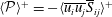
These shear layers are the source of additional production of TKE within the surface layer through the
 $-\overline{uv}~\unicode[STIX]{x2202}\bar{U}/\unicode[STIX]{x2202}y$
term, as shown in figures 5(a,b) and 6(a). This additional production of TKE, which is above and beyond the normal production of TKE in wall-bounded flows through the
$-\overline{uv}~\unicode[STIX]{x2202}\bar{U}/\unicode[STIX]{x2202}y$
term, as shown in figures 5(a,b) and 6(a). This additional production of TKE, which is above and beyond the normal production of TKE in wall-bounded flows through the
 $-\overline{uw}~\unicode[STIX]{x2202}\bar{U}/\unicode[STIX]{x2202}z$
term, dominates the overall production of TKE within the surface layer, as shown in figures 5(a,b,d,g) and 6(a,d,g). The additional production of TKE through these shear layers is dissipated by the turbulent eddies above the no-slip regions, as shown in figures 5(e,h) and 6(e,h), such that
$-\overline{uw}~\unicode[STIX]{x2202}\bar{U}/\unicode[STIX]{x2202}z$
term, dominates the overall production of TKE within the surface layer, as shown in figures 5(a,b,d,g) and 6(a,d,g). The additional production of TKE through these shear layers is dissipated by the turbulent eddies above the no-slip regions, as shown in figures 5(e,h) and 6(e,h), such that
 $$\begin{eqnarray}\{-\overline{uv}~\unicode[STIX]{x2202}\bar{U}/\unicode[STIX]{x2202}y\}_{shear\,layers}\sim \{\unicode[STIX]{x1D708}\overline{s_{ij}s_{ij}}\}_{no\text{-}slip}.\end{eqnarray}$$
An order of magnitude estimate of the terms in (3.3) leads to the scaling law for
 $U_{s}^{+}$
. Specifically, within the surface layer, the spanwise gradients of the mean streamwise velocity can be estimated as
$U_{s}^{+}$
. Specifically, within the surface layer, the spanwise gradients of the mean streamwise velocity can be estimated as
 $\unicode[STIX]{x2202}\bar{U}/\unicode[STIX]{x2202}y\sim U_{ss}/g$
, where
$\unicode[STIX]{x2202}\bar{U}/\unicode[STIX]{x2202}y\sim U_{ss}/g$
, where
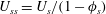 $U_{ss}=U_{s}/(1-\unicode[STIX]{x1D719}_{s})$
is the average slip velocity on the slip portions of the microtextured walls. Furthermore, the fluctuating strain rate above the no-slip regions can be estimated as
$U_{ss}=U_{s}/(1-\unicode[STIX]{x1D719}_{s})$
is the average slip velocity on the slip portions of the microtextured walls. Furthermore, the fluctuating strain rate above the no-slip regions can be estimated as
 $\{{s_{ij}\}}_{no-slip}\sim \sqrt{u_{\unicode[STIX]{x1D70F}_{n}}u_{\unicode[STIX]{x1D70F}}}/(\unicode[STIX]{x1D708}/\sqrt{u_{\unicode[STIX]{x1D70F}_{n}}u_{\unicode[STIX]{x1D70F}}})$
, where
$\{{s_{ij}\}}_{no-slip}\sim \sqrt{u_{\unicode[STIX]{x1D70F}_{n}}u_{\unicode[STIX]{x1D70F}}}/(\unicode[STIX]{x1D708}/\sqrt{u_{\unicode[STIX]{x1D70F}_{n}}u_{\unicode[STIX]{x1D70F}}})$
, where
 $\sqrt{u_{\unicode[STIX]{x1D70F}_{n}}u_{\unicode[STIX]{x1D70F}}}$
is the characteristic velocity of the turbulent eddies above the no-slip regions within the surface layer, estimated as the geometric average of the wall friction velocities
$\sqrt{u_{\unicode[STIX]{x1D70F}_{n}}u_{\unicode[STIX]{x1D70F}}}$
is the characteristic velocity of the turbulent eddies above the no-slip regions within the surface layer, estimated as the geometric average of the wall friction velocities
 $u_{\unicode[STIX]{x1D70F}_{n}}=u_{\unicode[STIX]{x1D70F}}/\sqrt{\unicode[STIX]{x1D719}_{s}}$
and
$u_{\unicode[STIX]{x1D70F}_{n}}=u_{\unicode[STIX]{x1D70F}}/\sqrt{\unicode[STIX]{x1D719}_{s}}$
and
 $u_{\unicode[STIX]{x1D70F}}$
above the no-slip regions at
$u_{\unicode[STIX]{x1D70F}}$
above the no-slip regions at
 $z=0$
and
$z=0$
and
 $z\sim g$
, respectively, and
$z\sim g$
, respectively, and
 $\unicode[STIX]{x1D708}/\sqrt{u_{\unicode[STIX]{x1D70F}_{n}}u_{\unicode[STIX]{x1D70F}}}$
is the associated inner length scale. Finally, the Reynolds shear stress
$\unicode[STIX]{x1D708}/\sqrt{u_{\unicode[STIX]{x1D70F}_{n}}u_{\unicode[STIX]{x1D70F}}}$
is the associated inner length scale. Finally, the Reynolds shear stress
 $-\overline{uv}$
can be estimated using a mixing-length model as
$-\overline{uv}$
can be estimated using a mixing-length model as
 $-\overline{uv}\sim \unicode[STIX]{x1D708}_{t}\unicode[STIX]{x2202}\bar{U}/\unicode[STIX]{x2202}y\sim u^{\prime }\ell ~\unicode[STIX]{x2202}\bar{U}/\unicode[STIX]{x2202}y$
, where
$-\overline{uv}\sim \unicode[STIX]{x1D708}_{t}\unicode[STIX]{x2202}\bar{U}/\unicode[STIX]{x2202}y\sim u^{\prime }\ell ~\unicode[STIX]{x2202}\bar{U}/\unicode[STIX]{x2202}y$
, where
 $u^{\prime }\sim \sqrt{u_{\unicode[STIX]{x1D70F}_{n}}u_{\unicode[STIX]{x1D70F}}}$
is the characteristic velocity of the largest eddies within the surface layer, and
$u^{\prime }\sim \sqrt{u_{\unicode[STIX]{x1D70F}_{n}}u_{\unicode[STIX]{x1D70F}}}$
is the characteristic velocity of the largest eddies within the surface layer, and
 $\ell \sim \sqrt{g\unicode[STIX]{x1D708}/u_{\unicode[STIX]{x1D70F}}}$
is their characteristic size, approximated as the geometric average of
$\ell \sim \sqrt{g\unicode[STIX]{x1D708}/u_{\unicode[STIX]{x1D70F}}}$
is their characteristic size, approximated as the geometric average of
 $g$
and
$g$
and
 $\unicode[STIX]{x1D708}/u_{\unicode[STIX]{x1D70F}}$
, representing the size of the largest eddies at
$\unicode[STIX]{x1D708}/u_{\unicode[STIX]{x1D70F}}$
, representing the size of the largest eddies at
 $z\sim g$
and
$z\sim g$
and
 $z\sim 0$
, respectively. Substitution of these expressions into (3.3) gives the scaling law for
$z\sim 0$
, respectively. Substitution of these expressions into (3.3) gives the scaling law for
 $U_{s}^{+}$
as
$U_{s}^{+}$
as
 $$\begin{eqnarray}\frac{\unicode[STIX]{x1D719}_{s}^{3/8}}{(1-\unicode[STIX]{x1D719}_{s})}\,U_{s}^{+}\sim \{{g^{+}\}}^{3/4}.\end{eqnarray}$$
Given that the dominant contribution to
 $(B-B_{0})$
arises from
$(B-B_{0})$
arises from
 $U_{s}^{+}$
, a similar scaling can also be assumed for
$U_{s}^{+}$
, a similar scaling can also be assumed for
 $(B-B_{0})$
:
$(B-B_{0})$
:
 $$\begin{eqnarray}\frac{\unicode[STIX]{x1D719}_{s}^{3/8}}{(1-\unicode[STIX]{x1D719}_{s})}\,(B-B_{0})\sim \{{g^{+}\}}^{3/4},\end{eqnarray}$$
with the understanding that the multiplicative coefficient in the expression for
 $(B-B_{0})$
would be smaller than that for
$(B-B_{0})$
would be smaller than that for
 $U_{s}^{+}$
.
$U_{s}^{+}$
.

Figure 7. The scaling of
 $U_{s}^{+}$
and
$U_{s}^{+}$
and
 $(B-B_{0})$
with surface microtexture parameters in turbulent flow with SH or LI walls: (a–d) present DNS data in turbulent channel flow with SH longitudinal microgrooves or SH aligned microposts at
$(B-B_{0})$
with surface microtexture parameters in turbulent flow with SH or LI walls: (a–d) present DNS data in turbulent channel flow with SH longitudinal microgrooves or SH aligned microposts at
 $Re_{\unicode[STIX]{x1D70F}_{0}}\approx 222$
and
$Re_{\unicode[STIX]{x1D70F}_{0}}\approx 222$
and
 $442$
,
$442$
,
 $1/64\leqslant \unicode[STIX]{x1D719}_{s}\leqslant 1/2$
,
$1/64\leqslant \unicode[STIX]{x1D719}_{s}\leqslant 1/2$
,
 $\unicode[STIX]{x1D703}_{p}=0^{\circ }$
and
$\unicode[STIX]{x1D703}_{p}=0^{\circ }$
and
 $-30^{\circ }$
; (e,f) DNS data from other investigators in turbulent channel flow with SH longitudinal microgrooves, LI longitudinal microgrooves or SH aligned microposts at
$-30^{\circ }$
; (e,f) DNS data from other investigators in turbulent channel flow with SH longitudinal microgrooves, LI longitudinal microgrooves or SH aligned microposts at
 $180\lesssim Re_{\unicode[STIX]{x1D70F}_{0}}\lesssim 590$
,
$180\lesssim Re_{\unicode[STIX]{x1D70F}_{0}}\lesssim 590$
,
 $1/36\leqslant \unicode[STIX]{x1D719}_{s}\leqslant 1/2$
. Symbols as in figure 3. Other symbols in (e,f):
$1/36\leqslant \unicode[STIX]{x1D719}_{s}\leqslant 1/2$
. Symbols as in figure 3. Other symbols in (e,f):
 $Re_{\unicode[STIX]{x1D70F}_{0}}\approx 180$
,
$Re_{\unicode[STIX]{x1D70F}_{0}}\approx 180$
,
 $\unicode[STIX]{x1D719}_{s}=1/8$
,
$\unicode[STIX]{x1D719}_{s}=1/8$
,
 $1/4$
,
$1/4$
,
 $1/2$
,
$1/2$
,  $Re_{\unicode[STIX]{x1D70F}_{0}}\approx 395$
,
$Re_{\unicode[STIX]{x1D70F}_{0}}\approx 395$
,
 $\unicode[STIX]{x1D719}_{s}=1/16$
,
$\unicode[STIX]{x1D719}_{s}=1/16$
,
 $1/8$
,
$1/8$
,
 $1/4$
,
$1/4$
,
 $1/2$
,
$1/2$
,  $Re_{\unicode[STIX]{x1D70F}_{0}}\approx 590$
,
$Re_{\unicode[STIX]{x1D70F}_{0}}\approx 590$
,
 $\unicode[STIX]{x1D719}_{s}=1/16$
,
$\unicode[STIX]{x1D719}_{s}=1/16$
,
 $1/8$
,
$1/8$
,
 $1/4$
,
$1/4$
,
 $1/2$
, SH longitudinal microgrooves,
$1/2$
, SH longitudinal microgrooves,
 $\unicode[STIX]{x1D703}_{p}=0^{\circ }$
(Park et al.
Reference Park, Park and Kim2013);
$\unicode[STIX]{x1D703}_{p}=0^{\circ }$
(Park et al.
Reference Park, Park and Kim2013);  $Re_{\unicode[STIX]{x1D70F}}\approx 195$
,
$Re_{\unicode[STIX]{x1D70F}}\approx 195$
,
 $\unicode[STIX]{x1D719}_{s}=1/64$
,
$\unicode[STIX]{x1D719}_{s}=1/64$
,
 $1/9$
,
$1/9$
,  $Re_{\unicode[STIX]{x1D70F}}\approx 400$
,
$Re_{\unicode[STIX]{x1D70F}}\approx 400$
,
 $\unicode[STIX]{x1D719}_{s}=1/36$
,
$\unicode[STIX]{x1D719}_{s}=1/36$
,
 $1/16$
,
$1/16$
,
 $1/9$
, SH aligned microposts,
$1/9$
, SH aligned microposts,
 $\unicode[STIX]{x1D703}_{p}=0^{\circ }$
(Seo & Mani Reference Seo and Mani2016).
$\unicode[STIX]{x1D703}_{p}=0^{\circ }$
(Seo & Mani Reference Seo and Mani2016). Figure 7(a–d) shows
 $U_{s}^{+}$
and
$U_{s}^{+}$
and
 $(B-B_{0})$
from the DNS studies summarized in table 1, compared to (3.4) and (3.5). At both
$(B-B_{0})$
from the DNS studies summarized in table 1, compared to (3.4) and (3.5). At both
 $Re_{\unicode[STIX]{x1D70F}_{0}}\approx 222$
and
$Re_{\unicode[STIX]{x1D70F}_{0}}\approx 222$
and
 $442$
, and for both
$442$
, and for both
 $\unicode[STIX]{x1D703}_{p}=0^{\circ }$
and
$\unicode[STIX]{x1D703}_{p}=0^{\circ }$
and
 $\unicode[STIX]{x1D703}_{p}=-30^{\circ }$
,
$\unicode[STIX]{x1D703}_{p}=-30^{\circ }$
,
 $U_{s}^{+}$
and
$U_{s}^{+}$
and
 $(B-B_{0})$
scale as
$(B-B_{0})$
scale as
 $\{{g^{+}\}}^{3/4}$
, while normalization with
$\{{g^{+}\}}^{3/4}$
, while normalization with
 $\unicode[STIX]{x1D719}_{s}^{3/8}/(1-\unicode[STIX]{x1D719}_{s})$
collapses the data from different
$\unicode[STIX]{x1D719}_{s}^{3/8}/(1-\unicode[STIX]{x1D719}_{s})$
collapses the data from different
 $\unicode[STIX]{x1D719}_{s}$
. Both
$\unicode[STIX]{x1D719}_{s}$
. Both
 $U_{s}^{+}$
and
$U_{s}^{+}$
and
 $(B-B_{0})$
are Reynolds number independent and only functions of the geometrical parameters of the surface microtexture in wall units, in agreement with the predictions of (3.4) and (3.5).
$(B-B_{0})$
are Reynolds number independent and only functions of the geometrical parameters of the surface microtexture in wall units, in agreement with the predictions of (3.4) and (3.5).
A best fit to the DNS data gives the multiplicative coefficients in the expressions for
 $U_{s}^{+}$
and
$U_{s}^{+}$
and
 $(B-B_{0})$
as
$(B-B_{0})$
as
 $$\begin{eqnarray}\displaystyle U_{s}^{+} & = & \displaystyle 0.52\{(1-\unicode[STIX]{x1D719}_{s})\unicode[STIX]{x1D719}_{s}^{-3/8}\}\{{g^{+}\}}^{3/4},\end{eqnarray}$$
 $$\begin{eqnarray}\displaystyle (B-B_{0}) & = & \displaystyle 0.41\{(1-\unicode[STIX]{x1D719}_{s})\unicode[STIX]{x1D719}_{s}^{-3/8}\}\{{g^{+}\}}^{3/4},\end{eqnarray}$$
with
 $p$
-values of 0.98, obtained from the Kolmogorov–Smirnov goodness of fit test.
$p$
-values of 0.98, obtained from the Kolmogorov–Smirnov goodness of fit test.
Figure 7(e,f) shows the comparison of (3.6) and (3.7) with available DNS data from other investigators, obtained in turbulent channel flows using SH longitudinal microgrooves (Park et al.
Reference Park, Park and Kim2013), SH aligned microposts (Seo & Mani Reference Seo and Mani2016) or LI longitudinal microgrooves at viscosity ratios of
 $N\equiv \unicode[STIX]{x1D707}_{o}/\unicode[STIX]{x1D707}_{i}=0.1,1,10,20,100$
(Fu et al.
Reference Fu, Arenas, Leonardi and Hultmark2017). Good agreement can be seen between the predictions of (3.6) and (3.7) and available DNS data from other investigators for both SH longitudinal microgrooves and SH aligned microposts as long as
$N\equiv \unicode[STIX]{x1D707}_{o}/\unicode[STIX]{x1D707}_{i}=0.1,1,10,20,100$
(Fu et al.
Reference Fu, Arenas, Leonardi and Hultmark2017). Good agreement can be seen between the predictions of (3.6) and (3.7) and available DNS data from other investigators for both SH longitudinal microgrooves and SH aligned microposts as long as
 $g^{+}<100$
. For
$g^{+}<100$
. For
 $g^{+}>100$
, both
$g^{+}>100$
, both
 $U_{s}^{+}$
and
$U_{s}^{+}$
and
 $(B-B_{0})$
saturate and branch off from the predictions of (3.6) and (3.7). This saturation has been attributed to the width of the microgrooves,
$(B-B_{0})$
saturate and branch off from the predictions of (3.6) and (3.7). This saturation has been attributed to the width of the microgrooves,
 $g^{+}$
, approaching the mean streak spacing of
$g^{+}$
, approaching the mean streak spacing of
 $\unicode[STIX]{x1D706}^{+}\sim 100$
in turbulent wall flows (Park et al.
Reference Park, Park and Kim2013). Presumably, for
$\unicode[STIX]{x1D706}^{+}\sim 100$
in turbulent wall flows (Park et al.
Reference Park, Park and Kim2013). Presumably, for
 $g^{+}\gtrsim 100$
, the dynamics of turbulence above the slip regions becomes independent of the dynamics of turbulence above the no-slip regions, and both
$g^{+}\gtrsim 100$
, the dynamics of turbulence above the slip regions becomes independent of the dynamics of turbulence above the no-slip regions, and both
 $U_{s}^{+}$
and
$U_{s}^{+}$
and
 $(B-B_{0})$
approach their limiting values.
$(B-B_{0})$
approach their limiting values.
Good agreement can also be seen in figure 7(e,f) between the predictions of (3.6) and (3.7) and DNS results in turbulent channel flows with LI longitudinal microgrooves (Fu et al.
Reference Fu, Arenas, Leonardi and Hultmark2017) when the viscosity ratio,
 $N$
, is greater than
$N$
, is greater than
 ${\sim}10$
. These results suggest that for high enough viscosity ratios, of
${\sim}10$
. These results suggest that for high enough viscosity ratios, of
 $N\gtrsim 10$
, the drag reduction of LI surfaces begins to approach that of SH surfaces. These findings are consistent with analytical solutions in laminar shear flow with LI surfaces obtained by Schönecker, Baier & Hardt (Reference Schönecker, Baier and Hardt2014), and reproduced in figure 8, which show that for LI longitudinal microgrooves of depth
$N\gtrsim 10$
, the drag reduction of LI surfaces begins to approach that of SH surfaces. These findings are consistent with analytical solutions in laminar shear flow with LI surfaces obtained by Schönecker, Baier & Hardt (Reference Schönecker, Baier and Hardt2014), and reproduced in figure 8, which show that for LI longitudinal microgrooves of depth
 $d=g$
,
$d=g$
,
 $\unicode[STIX]{x1D719}_{s}=0.5$
and viscosity ratio of
$\unicode[STIX]{x1D719}_{s}=0.5$
and viscosity ratio of
 $N=10$
, the effective slip length is
$N=10$
, the effective slip length is
 ${\approx}86\,\%$
of the effective slip length predicted by Philip’s solution (Philip Reference Philip1972) for the same surface microtexture with ‘idealized’, shear-free, SH interfaces. The LI results shown in figure 7(e,f) are also consistent with experimental measurements in turbulent Taylor–Couette flow with LI longitudinal microgrooves of depth
${\approx}86\,\%$
of the effective slip length predicted by Philip’s solution (Philip Reference Philip1972) for the same surface microtexture with ‘idealized’, shear-free, SH interfaces. The LI results shown in figure 7(e,f) are also consistent with experimental measurements in turbulent Taylor–Couette flow with LI longitudinal microgrooves of depth
 $d=g$
,
$d=g$
,
 $\unicode[STIX]{x1D719}_{s}=0.5$
and
$\unicode[STIX]{x1D719}_{s}=0.5$
and
 $0.7\leqslant N\leqslant 3.0$
(Van Buren & Smits Reference Van Buren and Smits2017), which show the drag reduction of the LI surface at
$0.7\leqslant N\leqslant 3.0$
(Van Buren & Smits Reference Van Buren and Smits2017), which show the drag reduction of the LI surface at
 $N\approx 2.0{-}3.0$
to be
$N\approx 2.0{-}3.0$
to be
 ${\approx}50{-}60\,\%$
of the drag reduction of a SH surface with the same surface microtexture.
${\approx}50{-}60\,\%$
of the drag reduction of a SH surface with the same surface microtexture.
In the derivation of (3.6) and (3.7), the multiplicative coefficients, of 0.52 and 0.41, were obtained based on DNS data which assumed ‘idealized’, shear-free boundaries at the air/water interfaces and, as such, did not consider the flow of air in the SH microgrooves. This raises a concern that the magnitudes of
 $U_{s}^{+}$
and
$U_{s}^{+}$
and
 $(B-B_{0})$
would be over-predicted by (3.6) and (3.7). An estimate of the degree of this over-prediction can be obtained by comparing analytical solutions for the effective slip length,
$(B-B_{0})$
would be over-predicted by (3.6) and (3.7). An estimate of the degree of this over-prediction can be obtained by comparing analytical solutions for the effective slip length,
 $L_{s,N}$
, obtained with a finite viscosity ratio,
$L_{s,N}$
, obtained with a finite viscosity ratio,
 $N$
, in laminar shear flow with LI longitudinal microgrooves (Schönecker et al.
Reference Schönecker, Baier and Hardt2014) to the effective slip length,
$N$
, in laminar shear flow with LI longitudinal microgrooves (Schönecker et al.
Reference Schönecker, Baier and Hardt2014) to the effective slip length,
 $L_{s,\infty }$
, which would be predicted in the same flow based on the assumption of shear-free liquid/air interfaces (Philip Reference Philip1972). Figure 8 shows
$L_{s,\infty }$
, which would be predicted in the same flow based on the assumption of shear-free liquid/air interfaces (Philip Reference Philip1972). Figure 8 shows
 $L_{s,N}/L_{s,\infty }$
as a function of
$L_{s,N}/L_{s,\infty }$
as a function of
 $N$
for longitudinal microgrooves of depth
$N$
for longitudinal microgrooves of depth
 $d=g$
and the range of solid fractions,
$d=g$
and the range of solid fractions,
 $1/64\leqslant \unicode[STIX]{x1D719}_{s}\leqslant 1/2$
, investigated in the present study. It can be seen that for
$1/64\leqslant \unicode[STIX]{x1D719}_{s}\leqslant 1/2$
, investigated in the present study. It can be seen that for
 $N\approx 56$
, corresponding to air/water interfaces, the ratio
$N\approx 56$
, corresponding to air/water interfaces, the ratio
 $L_{s,N}/L_{s,\infty }$
ranges from
$L_{s,N}/L_{s,\infty }$
ranges from
 $0.92\leqslant L_{s,N}/L_{s,\infty }\leqslant 0.97$
for
$0.92\leqslant L_{s,N}/L_{s,\infty }\leqslant 0.97$
for
 $1/64\leqslant \unicode[STIX]{x1D719}_{s}\leqslant 1/2$
. These results suggest that for the range of
$1/64\leqslant \unicode[STIX]{x1D719}_{s}\leqslant 1/2$
. These results suggest that for the range of
 $1/64\leqslant \unicode[STIX]{x1D719}_{s}\leqslant 1/2$
, considered in the present study, the errors in (3.6) and (3.7) due to the assumption of shear-free interfaces are no more than 10 %. These errors can become larger for solid fractions of
$1/64\leqslant \unicode[STIX]{x1D719}_{s}\leqslant 1/2$
, considered in the present study, the errors in (3.6) and (3.7) due to the assumption of shear-free interfaces are no more than 10 %. These errors can become larger for solid fractions of
 $\unicode[STIX]{x1D719}_{s}\lesssim 1/64$
or for shallow grooves of
$\unicode[STIX]{x1D719}_{s}\lesssim 1/64$
or for shallow grooves of
 $d\lesssim g/2$
(Schönecker et al.
Reference Schönecker, Baier and Hardt2014). However, such configurations of microgrooves are impractical to build, either because the microgroove blades become too thin to be structurally sustainable, or because the depth of the grooves becomes so shallow that the air/water interfaces can hit the bottom of the grooves during their deformation, thus expediting their collapse.
$d\lesssim g/2$
(Schönecker et al.
Reference Schönecker, Baier and Hardt2014). However, such configurations of microgrooves are impractical to build, either because the microgroove blades become too thin to be structurally sustainable, or because the depth of the grooves becomes so shallow that the air/water interfaces can hit the bottom of the grooves during their deformation, thus expediting their collapse.

Figure 8. Ratio of the effective slip length,
 $L_{s,N}$
, obtained with a finite viscosity ratio,
$L_{s,N}$
, obtained with a finite viscosity ratio,
 $N$
, based on the analytical solution of Schönecker et al. (Reference Schönecker, Baier and Hardt2014), to the effective slip length,
$N$
, based on the analytical solution of Schönecker et al. (Reference Schönecker, Baier and Hardt2014), to the effective slip length,
 $L_{s,\infty }$
, obtained with the assumption of shear-free liquid/air interfaces (Philip Reference Philip1972), in laminar shear flow over LI longitudinal microgrooves for groove depth
$L_{s,\infty }$
, obtained with the assumption of shear-free liquid/air interfaces (Philip Reference Philip1972), in laminar shear flow over LI longitudinal microgrooves for groove depth
 $d=g$
and
$d=g$
and
 $1/64\leqslant \unicode[STIX]{x1D719}_{s}\leqslant 1/2$
:
$1/64\leqslant \unicode[STIX]{x1D719}_{s}\leqslant 1/2$
:
 $\cdots \cdots$
,
$\cdots \cdots$
,
 $\unicode[STIX]{x1D719}_{s}=1/2$
; — ⋅ ⋅ —,
$\unicode[STIX]{x1D719}_{s}=1/2$
; — ⋅ ⋅ —,
 $\unicode[STIX]{x1D719}_{s}=1/8$
; — ⋅ —,
$\unicode[STIX]{x1D719}_{s}=1/8$
; — ⋅ —,
 $\unicode[STIX]{x1D719}_{s}=1/16$
; – – –,
$\unicode[STIX]{x1D719}_{s}=1/16$
; – – –,
 $\unicode[STIX]{x1D719}_{s}=1/32$
; ——,
$\unicode[STIX]{x1D719}_{s}=1/32$
; ——,
 $\unicode[STIX]{x1D719}_{s}=1/64$
.
$\unicode[STIX]{x1D719}_{s}=1/64$
.
Another concern is the effect of dynamic deformation of the interface on (3.6) and (3.7), as the multiplicative coefficients in (3.6) and (3.7) were obtained from DNS studies which were performed with ‘stationary’, flat or curved, shear-free interfaces. The effect of dynamic deformation of the interface can be assessed by examining available DNS results obtained with deformable interfaces, but pinned contact lines, in turbulent channel flows with LI longitudinal microgrooves at a viscosity ratio of
 $N=2.5$
for
$N=2.5$
for
 $We_{\unicode[STIX]{x1D70F}}=0$
and
$We_{\unicode[STIX]{x1D70F}}=0$
and
 $We_{\unicode[STIX]{x1D70F}}=0.024$
(Arenas-Navarro Reference Arenas-Navarro2017), where
$We_{\unicode[STIX]{x1D70F}}=0.024$
(Arenas-Navarro Reference Arenas-Navarro2017), where
 $We_{\unicode[STIX]{x1D70F}}\equiv \unicode[STIX]{x1D70C}_{o}u_{\unicode[STIX]{x1D70F}}\unicode[STIX]{x1D708}_{o}/\unicode[STIX]{x1D70E}$
is the Weber number,
$We_{\unicode[STIX]{x1D70F}}\equiv \unicode[STIX]{x1D70C}_{o}u_{\unicode[STIX]{x1D70F}}\unicode[STIX]{x1D708}_{o}/\unicode[STIX]{x1D70E}$
is the Weber number,
 $\unicode[STIX]{x1D70C}_{o}$
and
$\unicode[STIX]{x1D70C}_{o}$
and
 $\unicode[STIX]{x1D708}_{o}$
are the density and kinematic viscosity of the outer fluid, respectively, and
$\unicode[STIX]{x1D708}_{o}$
are the density and kinematic viscosity of the outer fluid, respectively, and
 $\unicode[STIX]{x1D70E}$
is the surface tension.
$\unicode[STIX]{x1D70E}$
is the surface tension.
Figure 9 shows
 $\{\unicode[STIX]{x1D719}_{s}^{3/8}/(1-\unicode[STIX]{x1D719}_{s})\}\,U_{s}^{+}$
and
$\{\unicode[STIX]{x1D719}_{s}^{3/8}/(1-\unicode[STIX]{x1D719}_{s})\}\,U_{s}^{+}$
and
 $\{\unicode[STIX]{x1D719}_{s}^{3/8}/(1-\unicode[STIX]{x1D719}_{s})\}\,(B-B_{0})$
computed from these DNS databases. Both
$\{\unicode[STIX]{x1D719}_{s}^{3/8}/(1-\unicode[STIX]{x1D719}_{s})\}\,(B-B_{0})$
computed from these DNS databases. Both
 $\{\unicode[STIX]{x1D719}_{s}^{3/8}/(1-\unicode[STIX]{x1D719}_{s})\}\,U_{s}^{+}$
and
$\{\unicode[STIX]{x1D719}_{s}^{3/8}/(1-\unicode[STIX]{x1D719}_{s})\}\,U_{s}^{+}$
and
 $\{\unicode[STIX]{x1D719}_{s}^{3/8}/(1-\unicode[STIX]{x1D719}_{s})\}\,(B-B_{0})$
can be seen to scale as
$\{\unicode[STIX]{x1D719}_{s}^{3/8}/(1-\unicode[STIX]{x1D719}_{s})\}\,(B-B_{0})$
can be seen to scale as
 ${\sim}{g^{+}\{}^{3/4}\}$
, in agreement with (3.6) and (3.7). However, the multiplicative coefficients in the best fit lines to the LI data are smaller than those in (3.6) and (3.7) by a factor of
${\sim}{g^{+}\{}^{3/4}\}$
, in agreement with (3.6) and (3.7). However, the multiplicative coefficients in the best fit lines to the LI data are smaller than those in (3.6) and (3.7) by a factor of
 $0.6$
for
$0.6$
for
 $U_{s}^{+}$
and a factor of
$U_{s}^{+}$
and a factor of
 $0.4$
for
$0.4$
for
 $(B-B_{0})$
. These factors are comparable to the ratio
$(B-B_{0})$
. These factors are comparable to the ratio
 $L_{s,N}/L_{s,\infty }=0.6$
observed for
$L_{s,N}/L_{s,\infty }=0.6$
observed for
 $N=2.5$
and
$N=2.5$
and
 $\unicode[STIX]{x1D719}_{s}=1/2$
in figure 8.
$\unicode[STIX]{x1D719}_{s}=1/2$
in figure 8.
The dynamic deformation of the interface is seen to have little effect on the slip velocity, with the values for
 $U_{s}^{+}$
at the two Weber numbers being nearly identical, as seen in figure 8(a). However, the surface ripples formed by the dynamic deformation of the interface can act as ‘surface roughness’ and reduce the magnitude of
$U_{s}^{+}$
at the two Weber numbers being nearly identical, as seen in figure 8(a). However, the surface ripples formed by the dynamic deformation of the interface can act as ‘surface roughness’ and reduce the magnitude of
 $(B-B_{0})$
by
$(B-B_{0})$
by
 $2.5-25.5\,\%$
at
$2.5-25.5\,\%$
at
 $We_{\unicode[STIX]{x1D70F}}=0.024$
compared to
$We_{\unicode[STIX]{x1D70F}}=0.024$
compared to
 $We_{\unicode[STIX]{x1D70F}}=0$
, as seen in figure 8(b). The results shown in figure 9 were obtained with LI longitudinal microgrooves at
$We_{\unicode[STIX]{x1D70F}}=0$
, as seen in figure 8(b). The results shown in figure 9 were obtained with LI longitudinal microgrooves at
 $N=2.5$
and pinned contact lines. As will be shown in § 4 (figure 12), for SH longitudinal microgrooves, a
$N=2.5$
and pinned contact lines. As will be shown in § 4 (figure 12), for SH longitudinal microgrooves, a
 $We_{\unicode[STIX]{x1D70F}}=0.024$
is very large and will lead to interface instability for
$We_{\unicode[STIX]{x1D70F}}=0.024$
is very large and will lead to interface instability for
 $g^{+}>6.5$
at
$g^{+}>6.5$
at
 $Re_{\unicode[STIX]{x1D70F}}\approx 200$
. Stable SH longitudinal microgrooves require much smaller values of
$Re_{\unicode[STIX]{x1D70F}}\approx 200$
. Stable SH longitudinal microgrooves require much smaller values of
 $We_{\unicode[STIX]{x1D70F}}$
, for which the effect of dynamic deformation of the interface on
$We_{\unicode[STIX]{x1D70F}}$
, for which the effect of dynamic deformation of the interface on
 $(B-B_{0})$
is much smaller than the results shown in figure 8(b). Nevertheless, these effects can be accounted for by constructing a
$(B-B_{0})$
is much smaller than the results shown in figure 8(b). Nevertheless, these effects can be accounted for by constructing a
 $\unicode[STIX]{x0394}B_{k}$
associated with the ‘roughness’ of the liquid/gas interface, and subtracting this
$\unicode[STIX]{x0394}B_{k}$
associated with the ‘roughness’ of the liquid/gas interface, and subtracting this
 $\unicode[STIX]{x0394}B_{k}$
from the
$\unicode[STIX]{x0394}B_{k}$
from the
 $(B-B_{0})$
given by (3.7) to get the drag reduction. More recent DNS studies (Rastegari & Akhavan Reference Rastegari and Akhavan2018b
) suggest that the motion of the contact line may be a more important source of roughness effects. A similar procedure can also be used to account for the roughness effects arising from the motion of the contact line on SH or LI longitudinal microgrooves or aligned microposts, assuming the interface has not fully collapsed.
$(B-B_{0})$
given by (3.7) to get the drag reduction. More recent DNS studies (Rastegari & Akhavan Reference Rastegari and Akhavan2018b
) suggest that the motion of the contact line may be a more important source of roughness effects. A similar procedure can also be used to account for the roughness effects arising from the motion of the contact line on SH or LI longitudinal microgrooves or aligned microposts, assuming the interface has not fully collapsed.

Figure 9. Effect of dynamic deformation of the interface on (a)
 $U_{s}^{+}$
and (b)
$U_{s}^{+}$
and (b)
 $(B-B_{0})$
, based on DNS results with deformable interfaces, but pinned contact lines, in turbulent channel flows with LI longitudinal microgrooves at
$(B-B_{0})$
, based on DNS results with deformable interfaces, but pinned contact lines, in turbulent channel flows with LI longitudinal microgrooves at
 $Re_{\unicode[STIX]{x1D70F}}\approx 180$
,
$Re_{\unicode[STIX]{x1D70F}}\approx 180$
,
 $\unicode[STIX]{x1D719}_{s}=1/2$
,
$\unicode[STIX]{x1D719}_{s}=1/2$
,
 $N=2.5$
(Arenas-Navarro Reference Arenas-Navarro2017):
$N=2.5$
(Arenas-Navarro Reference Arenas-Navarro2017):
 $We_{\unicode[STIX]{x1D70F}}=0$
;
$We_{\unicode[STIX]{x1D70F}}=0$
;  $We_{\unicode[STIX]{x1D70F}}=0.024$
.
$We_{\unicode[STIX]{x1D70F}}=0.024$
.Finally, it should be noted that, given that the derivations of (3.6) and (3.7) require an unobstructed passageway through the surface microtexture, these scalings are not expected to apply to staggered microposts or transverse microgrooves.
4 Sustainability bounds of superhydrophobic surfaces
Equations (3.1) and (3.7) provide a tool for a priori prediction of the magnitude of drag reduction with any pattern of SH longitudinal microgrooves or aligned microposts in turbulent flow at any Reynolds number. However, design of optimal SH surfaces also requires consideration of the sustainability bounds of such surfaces, as all SH surfaces are susceptible to a wetting transition from the Cassie–Baxter state to a Wenzel state. This wetting transition can occur because of (i) depinning of the contact line and/or sagging of the liquid–gas interface under high local pressures (Zheng et al. Reference Zheng, Yu and Zhao2005; Checco et al. Reference Checco, Ocko, Rahman, Black, Tasinkevych, Giacomello and Dietrich2014) or (ii) diffusion or entrainment of the gas layer into the working liquid under high local shear rates (Samaha et al. Reference Samaha, Tafreshi and Gad-el Hak2012; Karatay et al. Reference Karatay, Tsai and Lammertink2013; Wexler et al. Reference Wexler, Jacobi and Stone2015; Ling et al. Reference Ling, Katz, Fu and Hultmark2017) of turbulent flow. Of the two mechanisms, the wetting transition due to high local pressures is generally the first mode of failure, and of the different SH surface microtextures, longitudinal microgrooves are the most stable under this mode of failure, as impingement of the flow on the back of microposts creates large stagnation pressures which can expedite the wetting transition (Seo, García-Mayoral & Mani Reference Seo, García-Mayoral and Mani2015). Consequently, in this section we will focus only on the pressure stability bounds of SH longitudinal microgrooves.
For SH longitudinal microgrooves with stable interfaces, the contact line is pinned and the shape of the interface is governed by the Young–Laplace equation
 $$\begin{eqnarray}\unicode[STIX]{x0394}P=-\frac{\unicode[STIX]{x1D70E}}{R}=-\frac{2\unicode[STIX]{x1D70E}\cos (\unicode[STIX]{x1D703}_{c})}{g},\end{eqnarray}$$
where
 $\unicode[STIX]{x0394}P$
is the pressure difference across the interface,
$\unicode[STIX]{x0394}P$
is the pressure difference across the interface,
 $\unicode[STIX]{x1D70E}$
is the surface tension,
$\unicode[STIX]{x1D70E}$
is the surface tension,
 $R$
is the radius of curvature of the interface,
$R$
is the radius of curvature of the interface,
 $\unicode[STIX]{x1D703}_{c}$
is the contact angle and
$\unicode[STIX]{x1D703}_{c}$
is the contact angle and
 $g$
is the microgroove width. With increasing
$g$
is the microgroove width. With increasing
 $\unicode[STIX]{x0394}P$
, the contact angle increases until it reaches the maximum advancing contact angle,
$\unicode[STIX]{x0394}P$
, the contact angle increases until it reaches the maximum advancing contact angle,
 $\unicode[STIX]{x1D703}_{F,adv}$
, at which point the contact line depins (Checco et al.
Reference Checco, Ocko, Rahman, Black, Tasinkevych, Giacomello and Dietrich2014). Assuming a maximum advancing contact angle of
$\unicode[STIX]{x1D703}_{F,adv}$
, at which point the contact line depins (Checco et al.
Reference Checco, Ocko, Rahman, Black, Tasinkevych, Giacomello and Dietrich2014). Assuming a maximum advancing contact angle of
 $\unicode[STIX]{x1D703}_{F,adv}=120^{\circ }$
(Nishino et al.
Reference Nishino, Meguro, Nakamae, Matsushita and Ueda1999), the criterion for stability of SH interfaces becomes
$\unicode[STIX]{x1D703}_{F,adv}=120^{\circ }$
(Nishino et al.
Reference Nishino, Meguro, Nakamae, Matsushita and Ueda1999), the criterion for stability of SH interfaces becomes
 $\unicode[STIX]{x0394}Pg/\unicode[STIX]{x1D70E}\leqslant 1$
, or
$\unicode[STIX]{x0394}Pg/\unicode[STIX]{x1D70E}\leqslant 1$
, or
 $$\begin{eqnarray}(\unicode[STIX]{x0394}P^{+})(g^{+})(We_{\unicode[STIX]{x1D70F}})\leqslant 1,\end{eqnarray}$$
where
 $\unicode[STIX]{x0394}P^{+}\equiv \unicode[STIX]{x0394}P/(\unicode[STIX]{x1D70C}u_{\unicode[STIX]{x1D70F}}^{2})$
is the non-dimensional pressure, and
$\unicode[STIX]{x0394}P^{+}\equiv \unicode[STIX]{x0394}P/(\unicode[STIX]{x1D70C}u_{\unicode[STIX]{x1D70F}}^{2})$
is the non-dimensional pressure, and
 $We_{\unicode[STIX]{x1D70F}}\equiv \unicode[STIX]{x1D70C}u_{\unicode[STIX]{x1D70F}}\unicode[STIX]{x1D708}/\unicode[STIX]{x1D70E}$
is the Weber number.
$We_{\unicode[STIX]{x1D70F}}\equiv \unicode[STIX]{x1D70C}u_{\unicode[STIX]{x1D70F}}\unicode[STIX]{x1D708}/\unicode[STIX]{x1D70E}$
is the Weber number.

Figure 10. Probability density function and cumulative distribution function of the wall pressure fluctuations in turbulent channel flow with SH longitudinal microgrooves, compared to turbulent channel flow with smooth, no-slip walls: (a) probability density function,
 $f_{p}(p_{w}^{+}/\{\langle \overline{p^{2}}\rangle _{w}^{+}\!\}^{1/2})$
; (b) cumulative distribution function,
$f_{p}(p_{w}^{+}/\{\langle \overline{p^{2}}\rangle _{w}^{+}\!\}^{1/2})$
; (b) cumulative distribution function,
 $F_{p}(p_{w}^{+}/\{\langle \overline{p^{2}}\rangle _{w}^{+}\}^{1/2})$
; – – –, –
$F_{p}(p_{w}^{+}/\{\langle \overline{p^{2}}\rangle _{w}^{+}\}^{1/2})$
; – – –, –
 $\cdot$
–, SH longitudinal microgrooves,
$\cdot$
–, SH longitudinal microgrooves,
 $Re_{\unicode[STIX]{x1D70F}_{0}}\approx 442$
,
$Re_{\unicode[STIX]{x1D70F}_{0}}\approx 442$
,
 $\unicode[STIX]{x1D719}_{s}=1/64$
,
$\unicode[STIX]{x1D719}_{s}=1/64$
,
 $g^{+0}\approx 63$
,
$g^{+0}\approx 63$
,
 $\unicode[STIX]{x1D703}_{p}=0^{\circ }$
and
$\unicode[STIX]{x1D703}_{p}=0^{\circ }$
and
 $-30^{\circ }$
, respectively;
$-30^{\circ }$
, respectively;
 $\cdots \cdots$
, base turbulent channel flow with smooth, no-slip walls,
$\cdots \cdots$
, base turbulent channel flow with smooth, no-slip walls,
 $Re_{\unicode[STIX]{x1D70F}_{0}}\approx 442$
; —— (orange), Gaussian distribution.
$Re_{\unicode[STIX]{x1D70F}_{0}}\approx 442$
; —— (orange), Gaussian distribution.
Assessing the stability bounds of SH surfaces in turbulent flow from (4.2) requires a knowledge of
 $\unicode[STIX]{x0394}P^{+}$
. In turbulent flow,
$\unicode[STIX]{x0394}P^{+}$
. In turbulent flow,
 $\unicode[STIX]{x0394}P^{+}$
arises from the instantaneous pressure fluctuations on the SH walls. The range of values assumed by the instantaneous pressure fluctuations on the SH walls can be assessed by examining the probability density function (p.d.f.) of the wall pressure fluctuations,
$\unicode[STIX]{x0394}P^{+}$
arises from the instantaneous pressure fluctuations on the SH walls. The range of values assumed by the instantaneous pressure fluctuations on the SH walls can be assessed by examining the probability density function (p.d.f.) of the wall pressure fluctuations,
 $f_{p}(p_{w}^{+}/\{\langle \overline{p^{2}}\rangle _{w}^{+}\!\}^{1/2})$
. Figure 10(a) shows the p.d.f. of wall pressure fluctuations in turbulent channel flow with SH longitudinal microgrooves at
$f_{p}(p_{w}^{+}/\{\langle \overline{p^{2}}\rangle _{w}^{+}\!\}^{1/2})$
. Figure 10(a) shows the p.d.f. of wall pressure fluctuations in turbulent channel flow with SH longitudinal microgrooves at
 $Re_{\unicode[STIX]{x1D70F}_{0}}\approx 442$
,
$Re_{\unicode[STIX]{x1D70F}_{0}}\approx 442$
,
 $\unicode[STIX]{x1D719}_{s}=1/64$
,
$\unicode[STIX]{x1D719}_{s}=1/64$
,
 $g^{+0}\approx 63$
and
$g^{+0}\approx 63$
and
 $\unicode[STIX]{x1D703}_{p}=0^{\circ }$
and
$\unicode[STIX]{x1D703}_{p}=0^{\circ }$
and
 $\unicode[STIX]{x1D703}_{p}=-30^{\circ }$
, compared to turbulent channel flow with smooth, no-slip walls. The p.d.f. of instantaneous wall pressure fluctuations in turbulent channel flow with SH walls is found to be similar to that for smooth, no-slip walls. Both p.d.f.s follow a non-Gaussian distribution with exponential tails. Similar non-Gaussian distributions have also been reported experimentally in high Reynolds number turbulent boundary layers (Tsuji et al.
Reference Tsuji, Fransson, Alfredsson and Johansson2007). The probability that the instantaneous pressure fluctuations fall within a given range of values,
$\unicode[STIX]{x1D703}_{p}=-30^{\circ }$
, compared to turbulent channel flow with smooth, no-slip walls. The p.d.f. of instantaneous wall pressure fluctuations in turbulent channel flow with SH walls is found to be similar to that for smooth, no-slip walls. Both p.d.f.s follow a non-Gaussian distribution with exponential tails. Similar non-Gaussian distributions have also been reported experimentally in high Reynolds number turbulent boundary layers (Tsuji et al.
Reference Tsuji, Fransson, Alfredsson and Johansson2007). The probability that the instantaneous pressure fluctuations fall within a given range of values,
 $a\leqslant p_{w}^{+}/\{\langle \overline{p^{2}}\rangle _{w}^{+}\!\}^{1/2}<b$
, can be estimated from
$a\leqslant p_{w}^{+}/\{\langle \overline{p^{2}}\rangle _{w}^{+}\!\}^{1/2}<b$
, can be estimated from
 $F_{p}(b)-F_{p}(a)=\int _{a}^{b}f_{p}(\unicode[STIX]{x1D702})\,\text{d}\unicode[STIX]{x1D702}$
, where
$F_{p}(b)-F_{p}(a)=\int _{a}^{b}f_{p}(\unicode[STIX]{x1D702})\,\text{d}\unicode[STIX]{x1D702}$
, where
 $F_{p}$
is the cumulative distribution function. Figure 10(b) shows the cumulative distribution functions,
$F_{p}$
is the cumulative distribution function. Figure 10(b) shows the cumulative distribution functions,
 $F_{p}(p_{w}^{+}/\{\langle \overline{p^{2}}\rangle _{w}^{+}\!\}^{1/2})$
, for the cases shown in figure 10(a). Examination of these cumulative distribution functions shows that the probability of the instantaneous wall pressure fluctuations falling within
$F_{p}(p_{w}^{+}/\{\langle \overline{p^{2}}\rangle _{w}^{+}\!\}^{1/2})$
, for the cases shown in figure 10(a). Examination of these cumulative distribution functions shows that the probability of the instantaneous wall pressure fluctuations falling within
 $\pm 4\{\langle \overline{p^{2}}\rangle _{w}^{+}\!\}^{1/2}$
is
$\pm 4\{\langle \overline{p^{2}}\rangle _{w}^{+}\!\}^{1/2}$
is
 $99.75\,\%$
. These results are consistent with experimental measurements in turbulent boundary layer flows (Schewe Reference Schewe1983), which show a probability of
$99.75\,\%$
. These results are consistent with experimental measurements in turbulent boundary layer flows (Schewe Reference Schewe1983), which show a probability of
 $99.7\,\%$
for the wall pressure fluctuations never exceeding
$99.7\,\%$
for the wall pressure fluctuations never exceeding
 $4\{\overline{p^{2}}_{w}^{+}\!\}^{1/2}$
. Based on these results, an upper estimate for the magnitude of
$4\{\overline{p^{2}}_{w}^{+}\!\}^{1/2}$
. Based on these results, an upper estimate for the magnitude of
 $\unicode[STIX]{x0394}P^{+}$
can be obtained as
$\unicode[STIX]{x0394}P^{+}$
can be obtained as
 $\unicode[STIX]{x0394}P^{+}\approx 4\{\langle \overline{p^{2}}\rangle _{w,SH}^{+}\!\}^{1/2}$
, with
$\unicode[STIX]{x0394}P^{+}\approx 4\{\langle \overline{p^{2}}\rangle _{w,SH}^{+}\!\}^{1/2}$
, with
 $99.75\,\%$
confidence that the instantaneous wall pressure fluctuations will not exceed this value.
$99.75\,\%$
confidence that the instantaneous wall pressure fluctuations will not exceed this value.
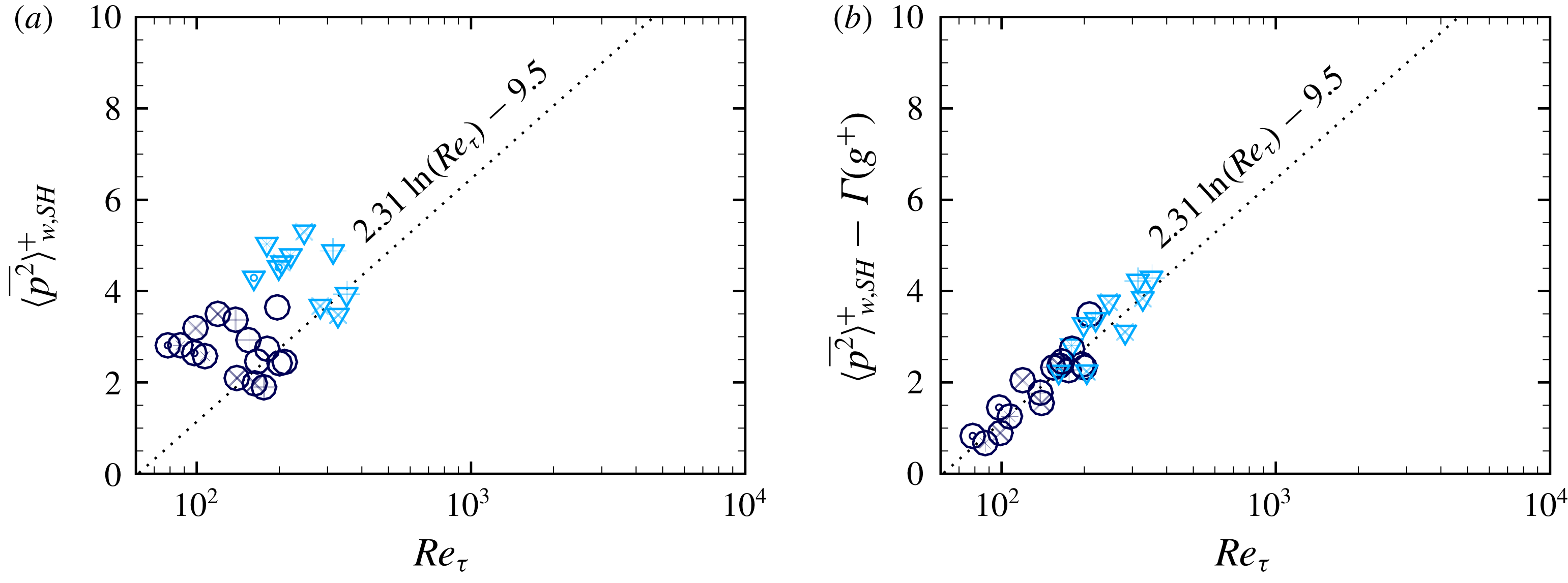
Figure 11. Mean-squared turbulent wall pressure fluctuations in turbulent channel flow with SH longitudinal microgrooves: (a)
 $\langle \bar{p^{2}}\rangle _{w,SH}^{+}$
as a function of
$\langle \bar{p^{2}}\rangle _{w,SH}^{+}$
as a function of
 $Re_{\unicode[STIX]{x1D70F}}$
; (b)
$Re_{\unicode[STIX]{x1D70F}}$
; (b)
 $\langle \bar{p^{2}}\rangle _{w,SH}^{+}-\unicode[STIX]{x1D6E4}(g^{+})$
as a function of
$\langle \bar{p^{2}}\rangle _{w,SH}^{+}-\unicode[STIX]{x1D6E4}(g^{+})$
as a function of
 $Re_{\unicode[STIX]{x1D70F}}$
, where
$Re_{\unicode[STIX]{x1D70F}}$
, where
 $\unicode[STIX]{x1D6E4}(g^{+})=2.32\ln (\{g^{+}\}^{3/4})-4.5$
. Symbols as in figure 3.
$\unicode[STIX]{x1D6E4}(g^{+})=2.32\ln (\{g^{+}\}^{3/4})-4.5$
. Symbols as in figure 3.
 $\cdots \cdots$
, the fit
$\cdots \cdots$
, the fit
 $\langle \bar{p^{2}}\rangle _{w,smooth}^{+}=2.31\ln (Re_{\unicode[STIX]{x1D70F}})-9.5$
, suggested by Sillero, Jiménez & Moser (Reference Sillero, Jiménez and Moser2013) for turbulent channel flows with smooth, no-slip walls.
$\langle \bar{p^{2}}\rangle _{w,smooth}^{+}=2.31\ln (Re_{\unicode[STIX]{x1D70F}})-9.5$
, suggested by Sillero, Jiménez & Moser (Reference Sillero, Jiménez and Moser2013) for turbulent channel flows with smooth, no-slip walls.
Figure 11(a) shows
 $\langle \overline{p^{2}}\rangle _{w,SH}^{+}$
as a function of
$\langle \overline{p^{2}}\rangle _{w,SH}^{+}$
as a function of
 $Re_{\unicode[STIX]{x1D70F}}$
from present DNS studies of turbulent channel flow with SH longitudinal microgrooves at fixed protrusion angle of
$Re_{\unicode[STIX]{x1D70F}}$
from present DNS studies of turbulent channel flow with SH longitudinal microgrooves at fixed protrusion angle of
 $\unicode[STIX]{x1D703}_{p}=-30^{\circ }$
(
$\unicode[STIX]{x1D703}_{p}=-30^{\circ }$
(
 $\unicode[STIX]{x1D703}_{c}=120^{\circ }$
). For reference, the fit
$\unicode[STIX]{x1D703}_{c}=120^{\circ }$
). For reference, the fit
 $\langle \overline{p^{2}}\rangle _{w,smooth}^{+}=2.31\ln (Re_{\unicode[STIX]{x1D70F}})-9.5$
, suggested by Sillero et al. (Reference Sillero, Jiménez and Moser2013), for turbulent channel flow with smooth no-slip walls is also shown. Similar to turbulent flow with smooth no-slip walls, the mean-squared wall pressure fluctuations in turbulent flow with SH walls is strongly Reynolds number dependent. However, due to the presence of spanwise slip, the magnitude of
$\langle \overline{p^{2}}\rangle _{w,smooth}^{+}=2.31\ln (Re_{\unicode[STIX]{x1D70F}})-9.5$
, suggested by Sillero et al. (Reference Sillero, Jiménez and Moser2013), for turbulent channel flow with smooth no-slip walls is also shown. Similar to turbulent flow with smooth no-slip walls, the mean-squared wall pressure fluctuations in turbulent flow with SH walls is strongly Reynolds number dependent. However, due to the presence of spanwise slip, the magnitude of
 $\langle \bar{p^{2}}\rangle _{w,SH}^{+}$
on SH walls is higher than that on smooth no-slip walls at comparable
$\langle \bar{p^{2}}\rangle _{w,SH}^{+}$
on SH walls is higher than that on smooth no-slip walls at comparable
 $Re_{\unicode[STIX]{x1D70F}}$
. Analysis of DNS data suggests that the effect of this spanwise slip can be captured in a function
$Re_{\unicode[STIX]{x1D70F}}$
. Analysis of DNS data suggests that the effect of this spanwise slip can be captured in a function
 $\unicode[STIX]{x1D6E4}(g^{+})$
, such that
$\unicode[STIX]{x1D6E4}(g^{+})$
, such that
 $$\begin{eqnarray}\langle \overline{p^{2}}\rangle _{w,SH}^{+}\approx \unicode[STIX]{x1D6E4}(g^{+})+\langle \overline{p^{2}}\rangle _{w,smooth}^{+}\approx \unicode[STIX]{x1D6E4}(g^{+})+2.31\ln (Re_{\unicode[STIX]{x1D70F}})-9.5.\end{eqnarray}$$
A best fit to the DNS data suggests the correlation
 $$\begin{eqnarray}\unicode[STIX]{x1D6E4}(g^{+})\approx \left\{\begin{array}{@{}ll@{}}2.32\ln (\{g^{+}\}^{3/4})-4.5,\quad & g^{+}\gtrsim 5\\ 0,\quad & g^{+}\lesssim 5.\end{array}\right.\end{eqnarray}$$
For
 $g^{+}\lesssim 5$
, the microgrooves become too narrow to generate any significant spanwise slip (Rastegari & Akhavan Reference Rastegari and Akhavan2018a
) and
$g^{+}\lesssim 5$
, the microgrooves become too narrow to generate any significant spanwise slip (Rastegari & Akhavan Reference Rastegari and Akhavan2018a
) and
 $\unicode[STIX]{x1D6E4}(g^{+})\approx 0$
. The correlations (4.3)–(4.4) fit the DNS data with a
$\unicode[STIX]{x1D6E4}(g^{+})\approx 0$
. The correlations (4.3)–(4.4) fit the DNS data with a
 $p$
-value of
$p$
-value of
 $0.97$
, based on the Kolmogorov–Smirnov goodness of fit test. Figure 11(b) shows the comparison of these correlations to the DNS data.
$0.97$
, based on the Kolmogorov–Smirnov goodness of fit test. Figure 11(b) shows the comparison of these correlations to the DNS data.

Figure 12. The maximum permissible
 $We^{+}$
and
$We^{+}$
and
 $g^{+}$
at a given
$g^{+}$
at a given
 $Re_{\unicode[STIX]{x1D70F}}$
to maintain the stability of SH longitudinal microgrooves in turbulent channel flow. Lines show the predictions of (4.2) for: ——,
$Re_{\unicode[STIX]{x1D70F}}$
to maintain the stability of SH longitudinal microgrooves in turbulent channel flow. Lines show the predictions of (4.2) for: ——,
 $Re_{\unicode[STIX]{x1D70F}}\approx 200$
; — —,
$Re_{\unicode[STIX]{x1D70F}}\approx 200$
; — —,
 $Re_{\unicode[STIX]{x1D70F}}\approx 400$
; – – –,
$Re_{\unicode[STIX]{x1D70F}}\approx 400$
; – – –,
 $Re_{\unicode[STIX]{x1D70F}}\approx 10^{3}$
; — ⋅ —,
$Re_{\unicode[STIX]{x1D70F}}\approx 10^{3}$
; — ⋅ —,
 $Re_{\unicode[STIX]{x1D70F}}\approx 10^{4}$
; –
$Re_{\unicode[STIX]{x1D70F}}\approx 10^{4}$
; –
 $\cdot$
 $\cdot$
–,
$\cdot$
–,
 $Re_{\unicode[STIX]{x1D70F}}\approx 10^{5}$
;
$Re_{\unicode[STIX]{x1D70F}}\approx 10^{5}$
;
 $\cdots \cdots$
,
$\cdots \cdots$
,
 $Re_{\unicode[STIX]{x1D70F}}\approx 10^{6}$
.
$Re_{\unicode[STIX]{x1D70F}}\approx 10^{6}$
.
Figure 12 shows the pressure stability bounds of SH longitudinal microgrooves obtained from (4.2), with
 $\unicode[STIX]{x0394}P^{+}$
approximated as
$\unicode[STIX]{x0394}P^{+}$
approximated as
 $\unicode[STIX]{x0394}P^{+}\approx 4\{\langle \overline{p^{2}}\rangle _{w,SH}^{+}\!\}^{1/2}$
and
$\unicode[STIX]{x0394}P^{+}\approx 4\{\langle \overline{p^{2}}\rangle _{w,SH}^{+}\!\}^{1/2}$
and
 $\langle \overline{p^{2}}\rangle _{w,SH}^{+}$
computed from (4.3) to (4.4). Due to the strong Reynolds number dependence of
$\langle \overline{p^{2}}\rangle _{w,SH}^{+}$
computed from (4.3) to (4.4). Due to the strong Reynolds number dependence of
 $\langle \overline{p^{2}}\rangle _{w,SH}^{+}$
, the pressure stability bounds of SH surfaces become significantly curtailed with increasing Reynolds number of the flow. Specifically, for the range of
$\langle \overline{p^{2}}\rangle _{w,SH}^{+}$
, the pressure stability bounds of SH surfaces become significantly curtailed with increasing Reynolds number of the flow. Specifically, for the range of
 $10^{4}\lesssim Re_{\unicode[STIX]{x1D70F}_{0}}\lesssim 10^{5}$
and
$10^{4}\lesssim Re_{\unicode[STIX]{x1D70F}_{0}}\lesssim 10^{5}$
and
 $We_{\unicode[STIX]{x1D70F}_{0}}\approx 5\times 10^{-3}$
, typical of practical applications, figure 3 shows that achieving
$We_{\unicode[STIX]{x1D70F}_{0}}\approx 5\times 10^{-3}$
, typical of practical applications, figure 3 shows that achieving
 ${\sim}50\,\%$
drag reduction requires a
${\sim}50\,\%$
drag reduction requires a
 $(B-B_{0})\approx 12{-}14$
. At the same time, figure 12 shows that the microgroove widths should be kept to
$(B-B_{0})\approx 12{-}14$
. At the same time, figure 12 shows that the microgroove widths should be kept to
 $g^{+}\lesssim 17{-}20$
to maintain the stability of the interface. The only way such large values of
$g^{+}\lesssim 17{-}20$
to maintain the stability of the interface. The only way such large values of
 $(B-B_{0})$
can be achieved with such small values of
$(B-B_{0})$
can be achieved with such small values of
 $g^{+}$
is by using ‘blade’ or ‘scalloped’ longitudinal microgrooves with
$g^{+}$
is by using ‘blade’ or ‘scalloped’ longitudinal microgrooves with
 $\unicode[STIX]{x1D719}_{s}\lesssim 0.02{-}0.05$
, per (3.7), where the nomenclature for ‘blade’ or ‘scalloped’ longitudinal microgrooves is borrowed from the riblet literature (Bechert et al.
Reference Bechert, Bruse, Hage, Van Der Hoeven and Hoppe1997).
$\unicode[STIX]{x1D719}_{s}\lesssim 0.02{-}0.05$
, per (3.7), where the nomenclature for ‘blade’ or ‘scalloped’ longitudinal microgrooves is borrowed from the riblet literature (Bechert et al.
Reference Bechert, Bruse, Hage, Van Der Hoeven and Hoppe1997).
The combination of (3.1), (3.7), (4.2) and (4.3)–(4.4) provides a set of design tools for a priori prediction of the magnitude of drag reduction and the sustainability bounds of SH surfaces in high Reynolds number turbulent flows. Given the Reynolds number,
 $Re_{\unicode[STIX]{x1D70F}_{0}}$
, and Weber number,
$Re_{\unicode[STIX]{x1D70F}_{0}}$
, and Weber number,
 $We_{\unicode[STIX]{x1D70F}_{0}}$
, of the base flow and a desired level of drag reduction, (3.1) provides an estimate of the required
$We_{\unicode[STIX]{x1D70F}_{0}}$
, of the base flow and a desired level of drag reduction, (3.1) provides an estimate of the required
 $(B-B_{0})$
, while (4.2) and (4.3)–(4.4) provide an estimate of the maximum groove width
$(B-B_{0})$
, while (4.2) and (4.3)–(4.4) provide an estimate of the maximum groove width
 $g^{+}$
for stability. These
$g^{+}$
for stability. These
 $(B-B_{0})$
and
$(B-B_{0})$
and
 $g^{+}$
values can then be used in (3.7) to determine the maximum allowable solid fraction,
$g^{+}$
values can then be used in (3.7) to determine the maximum allowable solid fraction,
 $\unicode[STIX]{x1D719}_{s}$
.
$\unicode[STIX]{x1D719}_{s}$
.
5 Summary and conclusions
Using scaling arguments and analysis of results from DNS, we present scaling laws which allow for a priori prediction of the magnitude of skin-friction drag reduction with SH or LI surfaces and the pressure stability bounds of SH surfaces in turbulent flow. It is shown that the magnitude of drag reduction can be parameterized in terms of the friction coefficient of the base flow and the shift,
 $(B-B_{0})$
, in the intercept of logarithmic-law representations of the mean velocity profiles in the flow with SH or LI walls compared to the base flow, where
$(B-B_{0})$
, in the intercept of logarithmic-law representations of the mean velocity profiles in the flow with SH or LI walls compared to the base flow, where
 $(B-B_{0})$
is Reynolds number independent. The parameterization of
$(B-B_{0})$
is Reynolds number independent. The parameterization of
 $(B-B_{0})$
in terms of the geometrical parameters of the SH or LI surface, and the pressure stability bounds of SH longitudinal microgrooves in turbulent flow are presented. It is shown that, for a given geometry and size of the surface microtexture in wall units, both the magnitude of drag reduction and the sustainability bounds of SH surfaces degrade with increasing Reynolds number of the base flow. Using these scalings, the narrow range of surface microtexture geometrical parameters which can yield large drag reduction while maintaining the stability of SH interfaces in high Reynolds number turbulent flows have been identified.
$(B-B_{0})$
in terms of the geometrical parameters of the SH or LI surface, and the pressure stability bounds of SH longitudinal microgrooves in turbulent flow are presented. It is shown that, for a given geometry and size of the surface microtexture in wall units, both the magnitude of drag reduction and the sustainability bounds of SH surfaces degrade with increasing Reynolds number of the base flow. Using these scalings, the narrow range of surface microtexture geometrical parameters which can yield large drag reduction while maintaining the stability of SH interfaces in high Reynolds number turbulent flows have been identified.
Acknowledgement
This work was supported by an unrestricted grant from the M. R. Prince Foundation, and NSF XSEDE Allocation TG-CTS070067N. This support is gratefully acknowledged.


