4.1 Accuracy of numerical results

In the STI simulations, the grid resolutions used for both the turbulence and the shock wave are critical to the accuracy of results. Here, the inflow turbulence is generated separately using $256^{3}$ grid points and has a $k_{max}\unicode[STIX]{x1D702}$ value of approximately 2.3, where $k_{max}$ is the maximum turbulence wavenumber and $\unicode[STIX]{x1D702}$ is the Kolmogorov length scale. The value of $k_{max}\unicode[STIX]{x1D702}$ is usually taken to be greater than 1.5 to resolve small-scale turbulence. It is relatively easy to construct a mesh to fully resolve turbulence in the preshock region. However, the postshock small-scale turbulence is expected to decrease in size, especially in the shock normal direction. Therefore, to ensure that the smallest postshock turbulence scales are well resolved, a detailed grid convergence test is conducted using five different meshes, as shown in table 1. The calculation of $k_{max}\unicode[STIX]{x1D702}$ is based on the largest grid size among all three directions to give safer and more conservative estimates.

In figure 3, several large- and small-scale turbulent statistics obtained from the convergence test are shown. The region of unsteady wrinkled shock movement is marked as a grey area in this and the following figures. Due to the unsteady shock movement and wrinkled shock surface, the averaged shock thickness is much larger than the instantaneous numerical shock thickness. As the mesh gets refined from grid-1 to grid-3 to grid-5 with the same compression ratio, all turbulent statistics converge, proving the sufficiency of the grid resolution. Results from meshes with different compression ratios, i.e. grid-5 and grid-4, are compared to make sure that the grid is fine enough to resolve the decreased length scale in the $x$ -direction. Statistics that characterize the behaviour of the mass fraction are also examined. Figure 4 shows the mass fraction variance and the Batchelor scale, representing large-scale and small-scale statistics of mixing respectively. Again, these statistics are grid converged and the errors are small when using grid-5. The convergence rate of the Batchelor scale is slower than for all of the other statistics, a consequence of VD effects.

Figure 4. Results of multi-fluid grid convergence tests at $Re_{\unicode[STIX]{x1D706}}=45$ and $M_{t}=0.09$ . (a) Mass fraction variance $\overline{\unicode[STIX]{x1D719}^{\prime }\unicode[STIX]{x1D719}^{\prime }}$ and (b) Batchelor scale  $\unicode[STIX]{x1D706}_{B}$ .

Larsson et al. (Reference Larsson, Bermejo-Moreno and Lele2013) have investigated how the large scales are affected by the finite computational box size. Their results show that the effects of box size are minimal for the range of parameters analysed. For the current study, the same peak wavenumber $k_{0}=4$ for the energy spectra and the same box size are used, so the effects from finite computational box size should also be negligible.

Another important issue in STI simulations is whether the interaction between the shock wave and the turbulence is well captured. When a shock-capturing scheme is used, a scale separation between the shock width and turbulence length scales is desirable. As suggested by Ryu & Livescu (Reference Ryu and Livescu2014), the ratio of the Kolmogorov length scale to the numerical shock width, $\unicode[STIX]{x1D6FF}_{n}$ , is considered to be an important parameter for assessment of this separation, where $\unicode[STIX]{x1D6FF}_{n}$ is calculated as $(u_{1,u}-u_{1,d})/|\unicode[STIX]{x2202}u_{1}/\unicode[STIX]{x2202}x_{1}|_{max}$ and $|\unicode[STIX]{x2202}u_{1}/\unicode[STIX]{x2202}x_{1}|_{max}$ denotes the maximum magnitude of the streamwise velocity gradient. For the coarsest simulation conducted with grid-1, the ratio of the preshock Kolmogorov length scale to the numerical shock width is estimated to have a value of approximately 0.93. However, since the Kolmogorov length scale is calculated using average dissipation, locally, turbulence eddies can become commensurate with the numerical shock thickness. Indeed, the use of instantaneous dissipation values to estimate the minimum turbulence length scale yields a ratio with the numerical shock thickness that is much smaller. In order to achieve a better scale separation, the numerical shock width needs to be reduced to a much smaller value than that corresponding to the grid-1 simulation. The dependence of $\unicode[STIX]{x1D6FF}_{n}$ on the grid size is investigated by conducting a series of tests using a range of grid sizes around the shock region. The results are shown in figure 5. This figure indicates that the numerical shock width is linearly correlated with the grid size, as expected. Therefore, by refining the mesh in the $x$ -direction, the scale separation can be controlled. Results from grid-2 and grid-3 simulations show good resolution of the postshock Kolmogorov length scale with a $k_{max}\unicode[STIX]{x1D702}$ value of approximately 1.45, but considerably different postshock prediction of $\overline{\unicode[STIX]{x1D714}_{2}^{\prime }\unicode[STIX]{x1D714}_{2}^{\prime }}$ . This difference can be attributed to the effects of the scale separation ratio (0.93 for grid-2 and 1.40 for grid-3), as shown in table 1. Further increase of the scale separation ratio has a small effect on the resolution of the postshock statistics, e.g. from grid-4 (1.4) to grid-5 (1.86). To confirm this, we have also considered another set of simulations with lower $Re_{\unicode[STIX]{x1D706}}$ but a wider range of scale separation ratios, and noticed that having a larger than 1.4 scale separation ratio has a minimal effect on the statistics presented here. These results are not shown for brevity. Based on these results, we can safely say that for the final simulation conducted with grid-5, which has a scale separation ratio of 1.86, the scale separation ratio is large enough to correctly resolve the STI with the current shock-capturing method.

Figure 5. Relation between the numerical shock width, $\unicode[STIX]{x1D6FF}_{n}$ , and the grid size in the shock region.

4.2 Convergence to the LIA for the single-fluid case

Using fully resolved STI simulations, Ryu & Livescu (Reference Ryu and Livescu2014), showed that as the ratio of Kolmogorov length scale, $\unicode[STIX]{x1D702}$ , to shock thickness, $\unicode[STIX]{x1D6FF}$ , becomes large, the DNS results converge to the LIA solutions. This suggests that the scale separation between $\unicode[STIX]{x1D702}$ and $\unicode[STIX]{x1D6FF}$ can be a criterion for controlling the viscous effects on the interaction. In Livescu & Ryu (Reference Livescu and Ryu2016), high-Reynolds-number/high-shock-Mach-number postshock turbulence data were generated using the LIA procedure, which resolved the issue of high or prohibitive computational cost of fully resolved DNS. For shock-capturing simulations, such convergence has not been investigated in previous studies. In DNS, the scale separation is controlled by the ratio $\unicode[STIX]{x1D702}/\unicode[STIX]{x1D6FF}$ , which can be calculated as $\unicode[STIX]{x1D702}/\unicode[STIX]{x1D6FF}=(Re_{\unicode[STIX]{x1D706}}^{0.5}(M_{s}-1))/(7.69M_{t})$ , and it was varied in Ryu & Livescu (Reference Ryu and Livescu2014) by changing $M_{t}$ , which also minimized the nonlinear effects. In shock-capturing simulations, $\unicode[STIX]{x1D702}/\unicode[STIX]{x1D6FF}_{n}$ , $M_{t}$ , $Re_{\unicode[STIX]{x1D706}}$ and $M_{s}$ are, in general, independent parameters; however, the same general principle can be applied to study the convergence of the numerical results to the LIA.

Unlike DNS, where an overlap between the shock width and turbulence scales does represent a physical problem, albeit different from the LIA limit, shock-capturing simulations need to have separation of scales to ensure that the numerical shock-capturing algorithm does not alter the physics of the problem. For the current simulations, the numerical shock thickness depends on the mesh size in the streamwise direction instead of any turbulent statistics, so it can be independently varied without changing $M_{t}$ and $Re_{\unicode[STIX]{x1D706}}$ . The shock thickness for different shock-capturing schemes is affected by the amount of numerical dissipation introduced around the shock. It is shown in Li & Jaberi (Reference Li and Jaberi2012) that the MP5 scheme has less numerical dissipation than the WENO scheme, so the numerical shock thickness is smaller for MP5. Generally, the shock jump is represented by 2–3 grid points and the numerical shock thickness calculated using $(u_{1,u}-u_{1,d})/|\unicode[STIX]{x2202}u_{1}/\unicode[STIX]{x2202}x_{1}|_{max}$ is approximately $1.6\unicode[STIX]{x0394}x$ . By changing $\unicode[STIX]{x0394}x$ , the scale separation ratio can be independently varied. Figures 3 and 4 (these figures correspond to multi-fluid cases, but the ideas are the same) show that for a ratio $\unicode[STIX]{x1D702}/\unicode[STIX]{x1D6FF}_{n}$ greater than 1.40, there is no significant error in the postshock statistics. Compared with shock-resolving simulations, this feature of shock-capturing simulations relaxes the requirement of a fully resolved shock profile and makes the simulations cheaper without diminishing the accuracy of the turbulent statistics. Larsson (Reference Larsson2010) took a different approach towards this problem. A theoretical model of the error introduced by the shock-capturing scheme was used to predict the postshock turbulence statistics. The error of the postshock Reynolds stresses was found to scale with the grid spacing to the second order. Using this model, a critical value of $k_{0}\unicode[STIX]{x0394}x$ can be calculated to control the error of the Reynolds stresses for a certain shock-capturing scheme. Compared with this method, the scale separation criterion naturally takes into account the artificial dissipation added in the shock region by using the numerical shock thickness as a shock length scale, which makes it a simpler criterion. Typically, a scale separation ratio $\unicode[STIX]{x1D702}/\unicode[STIX]{x1D6FF}_{n}\geqslant 1.4$ is recommended for the current shock-capturing simulations. We also recognize that, even though the scale separation ratio provides guidance in conducting shock-capturing turbulence-resolving simulations, the specific value of the scale separation criterion is not universal. It depends on the shock-capturing method and the way in which the numerical shock is quantified.

While $\unicode[STIX]{x1D702}/\unicode[STIX]{x1D6FF}_{n}$ is still an important parameter for assessment of the accuracy of the results, it is unlikely that the results in the shock region will have the same physical meaning as those from shock-resolving DNS. Therefore, to study the convergence to the LIA in shock-capturing simulations, $M_{t}$ and $Re_{\unicode[STIX]{x1D706}}$ need to be considered separately, instead of being one single parameter as in shock-resolving DNS. Single-fluid simulations are conducted covering a wide range of $M_{t}$ and $Re_{\unicode[STIX]{x1D706}}$ parameter space to study the convergence to the LIA. The value of $Re_{\unicode[STIX]{x1D706}}$ immediately upstream of the shock varies between 9 and 45, and $M_{t}$ immediately before the shock ranges from 0.03 to 0.38. More details on the LIA convergence tests can be found in table 2. The minimum scale separation in these tests is $\unicode[STIX]{x1D702}/\unicode[STIX]{x1D6FF}_{n}=1.4$ to ensure accuracy.

In figure 6, the streamwise and transverse Reynolds stress components ( $\overline{u_{1}^{\prime }u_{1}^{\prime }}$ and $\overline{u_{2}^{\prime }u_{2}^{\prime }}$ ) obtained from the single-fluid simulations are compared with the LIA solution. All of the plots are normalized by the values immediately upstream of the shock wave. The effects of $Re_{\unicode[STIX]{x1D706}}$ are first considered and the $M_{t}$ values are kept at approximately 0.24 (except for the $Re_{\unicode[STIX]{x1D706}}=45$ case, for which $M_{t}=0.09$ ). The results for $\overline{u_{1}^{\prime }u_{1}^{\prime }}$ are shown in figure 6(a). As $Re_{\unicode[STIX]{x1D706}}$ increases, the postshock peak values of $\overline{u_{1}^{\prime }u_{1}^{\prime }}$ converge to the LIA prediction in some region behind the shock. For $\overline{u_{2}^{\prime }u_{2}^{\prime }}$ , the postshock value reaches the peak immediately after the shock wave, and then it monotonically decreases. The peak value immediately after the shock can be affected by the shock thickness, shock corrugation and unsteady shock movement, so it is not a good representation of the shock amplification of turbulence. As suggested by Ryu & Livescu (Reference Ryu and Livescu2014), the values of $\overline{u_{2}^{\prime }u_{2}^{\prime }}$ at the corresponding $\overline{u_{1}^{\prime }u_{1}^{\prime }}$ peak positions are examined instead to evaluate the convergence. The trend of converging to the LIA prediction for $\overline{u_{2}^{\prime }u_{2}^{\prime }}$ is shown in figure 6(b), and this qualitatively matches with DNS results. However, compared with $\overline{u_{1}^{\prime }u_{1}^{\prime }}$ , the convergence of $\overline{u_{2}^{\prime }u_{2}^{\prime }}$ is slower. This can be explained by the fact that the $M_{t}$ values in these simulations are not low enough for $\overline{u_{2}^{\prime }u_{2}^{\prime }}$ to approximate the LIA solution. As $M_{t}$ increases, the shock wave becomes more wrinkled and it strongly affects the convergence of $\overline{u_{2}^{\prime }u_{2}^{\prime }}$ , since this quantity is more sensitive to shock wrinkling (Lee et al. Reference Lee, Lele and Moin1997).

Figure 6. Comparison of the Reynolds stress obtained from single-fluid simulations with the LIA results. Here, $M_{t}\approx 0.24$ except for $Re_{\unicode[STIX]{x1D706}}=45$ . (a) Streamwise Reynolds stress and (b) transverse Reynolds stress.

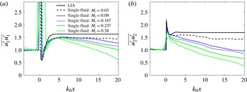
Figure 7. Comparison of the Reynolds stress obtained from single-fluid simulation with LIA results. Here, $Re_{\unicode[STIX]{x1D706}}\approx 30$ . (a) Streamwise Reynolds stress and (b) transverse Reynolds stress.

To further examine the role of the shock wrinkling, the effects of $M_{t}$ on the convergence to LIA predictions are examined by setting the $Re_{\unicode[STIX]{x1D706}}$ immediately before the shock wave to approximately 30 and varying $M_{t}$ . In figure 7, the normalized plots of Reynolds stresses are compared, and it can be seen that the amplification ratios of $\overline{u_{1}^{\prime }u_{1}^{\prime }}$ for all of the cases are very close (but different from the LIA limit), and those of $\overline{u_{2}^{\prime }u_{2}^{\prime }}$ converge to the LIA as $M_{t}$ decreases. This indicates that for the current shock-capturing simulations, the nonlinear effects induced by high $M_{t}$ are more important for $\overline{u_{2}^{\prime }u_{2}^{\prime }}$ than for $\overline{u_{1}^{\prime }u_{1}^{\prime }}$ . The results are also consistent with our previous statement that $\overline{u_{2}^{\prime }u_{2}^{\prime }}$ is more sensitive to $M_{t}$ . When comparing with DNS results, $\overline{u_{2}^{\prime }u_{2}^{\prime }}$ exhibits the same converging trend, but $\overline{u_{1}^{\prime }u_{1}^{\prime }}$ does not converge to the LIA limit at $Re_{\unicode[STIX]{x1D706}}=30$ . It seems that the LIA limit of $\overline{u_{1}^{\prime }u_{1}^{\prime }}$ cannot be approximated by decreasing $M_{t}$ at low $Re_{\unicode[STIX]{x1D706}}$ , and $Re_{\unicode[STIX]{x1D706}}$ needs to be large enough for convergence to be achieved. This is confirmed by another test with low $M_{t}$ (0.09) and higher $Re_{\unicode[STIX]{x1D706}}$ (45), as shown in figure 6. For $Re_{\unicode[STIX]{x1D706}}$ greater than 45 and $M_{t}$ lower than 0.1, the match to LIA results is fairly good, suggesting that a minimum value of $Re_{\unicode[STIX]{x1D706}}$ of approximately 45 is needed for the streamwise Reynolds stress component to converge.

In summary, the results show that the shock-capturing simulations exhibit a similar converging trend to the LIA solutions to shock-resolving DNS. The LIA solutions for individual Reynolds stresses can be approached provided that there is separation of scale between the turbulence scales and the shock width, $Re_{\unicode[STIX]{x1D706}}$ is large enough (for $\overline{u_{1}^{\prime }u_{1}^{\prime }}$ ) and $M_{t}$ is low enough (for $\overline{u_{2}^{\prime }u_{2}^{\prime }}$ ). On the other hand, the approach to the LIA prediction is different for the streamwise and spanwise components of the Reynolds stress tensor. For the transverse component, the converging trend agrees very well with the DNS results as we vary either $M_{t}$ or $Re_{\unicode[STIX]{x1D706}}$ . However, the streamwise component does not converge to the LIA prediction at low Reynolds numbers by varying $M_{t}$ , which is different from the DNS study by Ryu & Livescu (Reference Ryu and Livescu2014). This is attributed to the fundamental differences between shock-capturing turbulence-resolving simulations and shock-resolving DNS. A further test then shows that the LIA limit of $\overline{u_{1}^{\prime }u_{1}^{\prime }}$ can be approached at both large $Re_{\unicode[STIX]{x1D706}}$ (45) and low $M_{t}$ (0.09), which represents a regime where viscous and nonlinear effects are not important for the prediction of $\overline{u_{1}^{\prime }u_{1}^{\prime }}$ . Based on these findings, it would be safer to extend the single-fluid STI to multi-fluid STI at higher $Re_{\unicode[STIX]{x1D706}}$ . The requirement on $Re_{\unicode[STIX]{x1D706}}$ makes the shock-capturing simulation more expensive. However, one can still achieve a large-scale separation between the Kolmogorov length scale and the physical shock thickness with the shock-capturing method using coarser grids than shock-resolving DNS. In practice, the use of coarser grids for simulating the shock should dominate over the requirement of increased grid resolution for the turbulence to be able to capture a higher-Reynolds-number flow. Therefore, shock-capturing simulations should be an effective tool for studying STI so long as the results have been carefully verified as done here.

4.3 Effects of density variations on STI

In this section, the effects of density variations on STI are examined in detail by comparing the results obtained from VD or ‘multi-fluid’ simulations with those obtained from a reference ‘single-fluid’ simulation. As demonstrated in the previous section, a minimum value of $Re_{\unicode[STIX]{x1D706}}\approx 45$ is needed for the streamwise Reynolds stress to converge to the LIA prediction. At lower $Re_{\unicode[STIX]{x1D706}}$ , the convergence trend of $\overline{u_{1}^{\prime }u_{1}^{\prime }}$ is different from that for fully resolved DNS studies (Ryu & Livescu Reference Ryu and Livescu2014). Therefore, the value of $Re_{\unicode[STIX]{x1D706}}=45$ was chosen for the results presented in the rest of the paper. These results are obtained using grid-5 from table 1 and are grid converged, as shown in § 4.1. For the two multi-fluid cases considered in this study, two different methods are used to generate density variations at the inflow: (i) the heavy-fluid mole fraction is correlated with the random scalar used for initialization and (ii) the heavy-fluid mass fraction is correlated with the random scalar. In the following discussion, these two cases will be referred to as the multi-fluid A and multi-fluid B cases. The random scalar fields used to generate density in both multi-fluid cases are the same and have symmetric p.d.f.s. Evidently, this initialization of the density field will make the density p.d.f. of multi-fluid A case symmetrical and that of multi-fluid B case asymmetrical. Below, the multi-fluid A case will be treated as the default case, because it is a better representation of most mixing processes, in which the initial volumes occupied by the fluids in the mixture are specified. Moreover, the reactants in a stoichiometric combustion process are commonly introduced based on their mole fractions, so a specified mole fraction field at the inlet is preferred. The multi-fluid B case is also of interest to us, as it features a different inflow density structure (for the same density ratio), compared with the default case. The single-fluid reference simulation was conducted using the same inflow conditions for turbulent variables except density. In this reference case, the mass fraction of the heavy fluid is set to 1.0. At the same time, a passive scalar equation, which is the same as the mass fraction equation in the multi-fluid case, is solved for comparison. This case is referred to as just the single-fluid case and is used as a reference to study the effects of VD on STI. For all cases, the turbulence is allowed to adjust itself to the scalar field in the preshock region before interacting with the normal shock.

Figure 8. Two-dimensional (2-D) contours of the instantaneous scalar and density fields for (a,b) multi-fluid A simulation and (c,d) single-fluid simulation. The 2-D contours are taken at the same time step, in planes  $x{-}z$ .

In figure 2(b,c), the instantaneous shock fronts coloured by the ratio of the local pressure jump as obtained from the multi-fluid A and single-fluid cases are compared. As expected, the shock wave becomes more wrinkled and creates a stronger pressure jump in the multi-fluid case. Figure 8 shows the instantaneous 2-D contours of density and scalar for the multi-fluid A (heavy-fluid mole fraction) and single-fluid cases. After scaling the contours to the same range, figure 8(a,c) shows that the density variation is much stronger in the multi-fluid case due to the compositional change. In contrast, the variation of density in the reference (single-fluid) case results from thermodynamic fluctuation, which makes it very small for the parameters considered here. When examining the passive scalar and mass fraction fields (figure 8 b,d) for each case, we observe that the scalar fields have similar structure and magnitude before the shock wave as they are generated similarly at inflow. After passing through the shock wave, the scalar fields and mixing are different. Evidently, when the density variation is significant in preshock turbulence, the mixing enhancement by the shock is stronger.

Figures 9–15 show several important flow statistics obtained from the multi-fluid and single-fluid simulations. These statistics are gathered by averaging over homogeneous directions and time, so that they only depend on the streamwise direction.

Four important turbulence statistics are compared in figure 9 for the single-fluid and multi-fluid A cases. Before the shock wave, both cases yield the same results. This observation not only confirms that the inflow conditions are somewhat similar in these cases, but also implies that for the current simulation, the effect of density variations on turbulence is small in the preshock region. On comparing the multi-fluid TKE and vorticity variance with the corresponding single-fluid values in figure 9(a,d), it is noted that the amplification in these turbulent statistics is much more significant in the multi-fluid cases. Furthermore, the multi-fluid TKE reaches a peak at approximately $k_{0}x\approx 2.0$ , which is closer to the shock than $k_{0}x\approx \unicode[STIX]{x03C0}$ for the single-fluid case. Figure 9(b,c) shows the comparison for the streamwise turbulence Taylor micro length scale, $\unicode[STIX]{x1D706}_{1}$ , and the Kolmogorov length scale, $\unicode[STIX]{x1D702}$ . The reduction in turbulence length scales across the shock wave is evident in this figure; the multi-fluid cases show more reduction than the single-fluid case. It should be noted that the changes in turbulence statistics in the multi-fluid cases are expected to depend on the scalar structure and the Atwood number (e.g. Lombardini et al. Reference Lombardini, Hill, Pullin and Meiron2011); these are not discussed in this paper.

Figure 9. Plots of (a) TKE, (b) Kolmogorov length scale, (c) Taylor microscale and (d) transverse vorticity variance for the multi-fluid A (red) and single-fluid (blue) simulations.

Figure 10. Plots of normalized (a) scalar variance and (b) Batchelor scale for the multi-fluid A (red) and single-fluid (blue) simulations.

In figure 10, statistics related to the scalar field (heavy-fluid mass fraction for multi-fluid case A and passive scalar for the single-fluid case) and mixing are compared. Both the scalar variance $\overline{\unicode[STIX]{x1D719}^{\prime }\unicode[STIX]{x1D719}^{\prime }}$ and the Batchelor scale $\unicode[STIX]{x1D706}_{B}$ are shown. Here, $\unicode[STIX]{x1D706}_{B}$ is calculated based on the scalar dissipation and is representative of the smallest scales in the scalar field. The scalar statistics are normalized by the values immediately before the shock wave. After passing through the shock wave, the faster decay of the scalar variance for the multi-fluid case indicates stronger shock enhancement of scalar mixing. The Batchelor scale, however, shows a more complex behaviour. Unlike the Kolmogorov length scale, the Batchelor scale across the shock wave is observed to decrease with the same rate in the multi-fluid and single-fluid cases. After passing through the shock wave, the Batchelor scales of the multi-fluid cases exhibit a transient process of decreasing before returning to the preshock value, during which an even smaller structure of the scalar field is generated. In the single-fluid case, however, the Batchelor scale increases monotonically back to its preshock value. We also note that after $k_{0}x\approx 10.0$ , the multi-fluid $\unicode[STIX]{x1D706}_{B}$ values are larger than the single-fluid values as the faster mixing immediately after the shock smooths out the small scalar scales. The different behaviours of the scalar variance and the Batchelor scale in the postshock region can be explained by using the scalar transport equation. This will be discussed in § 4.5. We also note that results from multi-fluid case B show almost the same behaviour as those from multi-fluid case A for the above statistics, despite their completely different density p.d.f.s.

It was shown in figure 1 that the turbulence structure is affected very differently by the shock in regions with different density values. To further understand this behaviour, conditional expectations of several turbulence quantities, conditioned on the density, are calculated and examined. Figures 11–15 show these conditional means at various locations for the multi-fluid A and single-fluid cases. These statistics are calculated in selected spanwise planes ( $y{-}z$  planes) and then averaged in time. The conditional mean of the scalar, shown in figure 11(a), confirms the correlation of the density field with the scalar field (heavy-fluid mole fraction in this case). The dependence of the mole fraction on the density is almost linear on average, which suggests that the density fluctuations are mainly caused by compositional variations, instead of thermodynamic fluctuations. After passing through the shock wave, a decrease in the slope is observed due to enhancement of density variation across the shock wave, which is translated into an increased extent of the $x$ -axis values. This results from a larger local variation of the shock strength, with the subsequent amplification of the postshock values in the multi-fluid case. For comparison, figure 11(b) shows that the correlation between the passive scalar and the density is very low in the single-fluid case, which is expected.

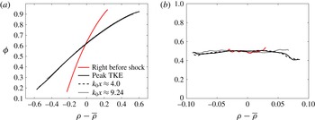
Figure 11. Conditional expectation of scalar as a function of density at various streamwise locations for (a) the multi-fluid A case and (b) the single-fluid case. The conditional mean is calculated using variables in a spanwise plane at certain streamwise locations and then averaged over time. The peak TKE positions are different between the multi-fluid ( $k_{0}x\approx 2.0$ ) and single-fluid ( $k_{0}x\approx \unicode[STIX]{x03C0}$ ) cases.

Figure 12. Conditional expectation of pressure as a function of density at various streamwise locations for (a) multi-fluid A close to the shock, (b) multi-fluid A at the far field and (c) the single-fluid case.

Figure 12 shows the development of the correlation between pressure and density fluctuations as the flow passes through the shock and moves away from it. Little correlation between the pressure and the density is observed before the shock, as expected. The increase in the correlation between the pressure and the density can be mostly attributed to the acoustic field. Due to the rapidly evolving nature of the acoustic field in STI (as evidenced in the rapid decay predicted by the LIA), it is worth comparing the pressure–density correlation close to the shock, where the transient effects dominate, with the far field behaviour. Figure 12(a) shows the development of the conditional mean of the pressure close to the shock wave. Immediately after the shock, at $k_{0}x\approx 0.64$ , there exists a strong positive correlation, which is the direct effect of the shock wave on the turbulence. During the postshock flow/turbulence development, the root-mean-square value of the pressure fluctuations, $p_{rms}^{\prime }$ , decreases rapidly, as indicated by the decreasing range of pressure fluctuations. This behaviour is related to the conversion of potential energy to TKE as evident by the fact that $p_{rms}^{\prime }$ remains almost unchanged after reaching the peak TKE position. In the far field (as shown in figure 12 b), the pressure fluctuations become less correlated with the density fluctuations in the mixed-fluid regions. The loss of pressure–density correlation is hypothesized to be caused by the nonlinearity introduced by the strong density fluctuations and the coupling between different modes.

Figure 12(c) shows the density–pressure correlation at various positions for the single-fluid case. In contrast to the multi-fluid case, the small-perturbation assumption is satisfied, so the mode decomposition of Kovasznay (Reference Kovasznay1953) can be applied. Based on the way in which the inflow turbulence is generated (Ristorcelli & Blaisdell Reference Ristorcelli and Blaisdell1997), the preshock turbulence is dominated by vorticity and acoustic modes. In this case, the pressure and density fluctuations should follow the isentropic process, $\unicode[STIX]{x1D6FE}(\unicode[STIX]{x1D6FE}-1)\unicode[STIX]{x1D70C}^{\prime }/\overline{\unicode[STIX]{x1D70C}}=(\unicode[STIX]{x1D6FE}-1)p^{\prime }/\overline{p}$ (Kovasznay Reference Kovasznay1953). For the current single-fluid case, the density and pressure fluctuations indeed follow the isentropic process scaling after being normalized by the local mean, in agreement with previous studies (Lee et al. Reference Lee, Lele and Moin1993; Mahesh et al. Reference Mahesh, Lele and Moin1997). After passing through the shock wave, the isentropic scaling is no longer satisfied due to the generation of an entropy mode, which has a negative correlation between density and temperature fluctuations (figure 13 b). This should be contrasted with the study by Mahesh et al. (Reference Mahesh, Lele and Moin1997), where the focus was on the interaction between the turbulent boundary layer and the shock wave. In such a case, the inflow fluctuations satisfy the weak form of Morkovin’s hypothesis (Morkovin Reference Morkovin and Favre1962), instead of following the isentropic relations. For the current case, despite the generation of an entropy mode, the pressure fluctuations cannot be neglected even at $k_{0}x=9.24$ , and, therefore, Morkovin’s hypothesis is not satisfied throughout the domain.

Figure 13. Conditional expectation of temperature as a function of density at various streamwise locations for (a) the multi-fluid A case and (b) the single-fluid case.

For a complete discussion on thermodynamic properties, the conditional expectation of temperature for both the multi-fluid A case and the single-fluid case are shown in figure 13. For the multi-fluid case, the direct effect of upstream Mach number fluctuations on the temperature is strong, resulting in a positive correlation between the density and the temperature. The generated entropy mode as predicted by the LIA in the single-fluid case seems to be overshadowed by this effect even further downstream. For the single-fluid case, the scaling between the density and the temperature fluctuations satisfies that of an isentropic process before the shock wave. Through the interaction with the shock wave, negative correlation is established, as previously mentioned. However, the correlation is not fully linear, which can be attributed to the presence of the acoustic mode and the coupling between this and the entropy mode.

Figure 14. Conditional expectation of TKE as a function of density at various streamwise locations for (a) the multi-fluid A case and (b) the single-fluid case.

Figure 15. Conditional expectation of enstrophy as a function of density at various streamwise locations for (a) the multi-fluid A case and (b) the single-fluid case.

In figure 14(a), the conditional expectation of the TKE is shown. We note that the TKE has a preferential distribution in the relatively high- or low-density regions in the postshock region. One possible explanation is that in the high- and low-density regions, the local sound speed has different values from that of the average sound speed, so that the local shock velocity, $u_{1,s}$ , becomes non-zero (in the reference frame of the laminar shock wave) and changes significantly. The local movement of the shock surface then further changes the postshock velocity, $u_{1,d}$ , and makes it deviate from the averaged postshock velocity, $\overline{u_{1,d}}$ . The deviation from $\overline{u_{1,d}}$ or $u_{i}^{\prime }$ in low- and high-density regions is much larger in magnitude than that in regions with moderate density, which results in larger TKE in the high- and low-density regions. We have computed the conditional average of $u_{i}^{\prime }$ on density. The results agree very well with our explanation for conditional TKE. We also note that the TKE is larger in the light-fluid regions compared with the heavy-fluid regions. This is due to the low inertia of the light fluid, which responds faster to changes in the local strain and, thus, accelerates faster (Livescu & Ristorcelli Reference Livescu, Ristorcelli and Eckhardt2009; Livescu et al. Reference Livescu, Ristorcelli, Petersen and Gore2010). This explanation is also applicable to figure 14(b) for the single-fluid case, which shows a preferential distribution of TKE in the lower-density fluid region before the shock wave. After passing through the shock wave, a stronger amplification in the high- and low-density regions is noted, but this is relatively weak, which agrees with the previous arguments.

The correlation between vorticity and density has a completely different behaviour from the TKE. Evidently, figure 15(a) shows that more vorticity is generated in the mixed-fluid regions. Before reaching the shock wave, the mixing process is relatively slow, so that there are still large regions with pure or partially mixed fluids and only narrow regions with fully mixed fluids. In these regions, the density gradients remain large. Through the interaction with the shock wave, the large density gradients lead to the generation of vorticity through the baroclinic torque (see (4.2)). For the single-fluid case (figure 15 b), the distribution of vorticity is not affected much by the shock because of the absence of large density variations.

The discussion above using conditional expectations emphasizes the VD effects on the modification of the turbulence structure. These effects reveal the underlying physics of multi-fluid STI. It is worth mentioning that the conditional expectations for the multi-fluid B case (not shown) show similar trends to those of the multi-fluid A case.

4.4 Reynolds stresses

The modification of the Favre-averaged normal Reynolds stress components $\widetilde{u_{\unicode[STIX]{x1D6FC}}^{\prime \prime }u_{\unicode[STIX]{x1D6FC}}^{\prime \prime }}$ or $R_{\unicode[STIX]{x1D6FC}\unicode[STIX]{x1D6FC}}$ (no summation over $\unicode[STIX]{x1D6FC}$ ) across the shock wave is an important feature of STI. As mentioned in the previous section, the preshock behaviour of the Reynolds stresses is very similar for multi-fluid and single-fluid cases and is dominated by viscous dissipation. The VD effects on the viscous dissipation in the pre-shock region are small at the Atwood number considered here. After passing through the shock wave, the main contributing mechanisms to the transient development of Reynolds stresses are the pressure–velocity correlation and the pressure–strain correlation (Lee et al. Reference Lee, Lele and Moin1997; Jamme et al. Reference Jamme, Cazalbou, Torres and Chassaing2002; Larsson et al. Reference Larsson, Bermejo-Moreno and Lele2013). This corresponds to the decay of the acoustic mode generated by STI. However, when the VD effect is introduced, the dominant terms in the Reynolds stress budgets are unknown, especially after passing through the shock wave. To investigate this, the budgets of the Favre-averaged normal Reynolds stresses need to be considered. Before further discussing the turbulence budgets, we need to differentiate the modification of turbulence by the shock from its evolution away from the shock. For shock-capturing simulations, when there is an overlap in scale, the turbulence and TKE budgets in the shock region cannot be correctly captured. However, when there is a scale separation between the shock and the turbulence, as is the case here, the numerical diffusion effects become, in principle, negligible during the interaction. Thus, the interaction becomes physical; however, it also becomes uninteresting from the point of view of the budget equations. Nevertheless, the evolution away from the shock is accurately described by the current approach and, for the VD case, has unknown evolution mechanisms that can be elucidated by the budget equations. Thus, the following discussion is focused on the evolution of turbulence away from the shock, with the immediate postshock value treated as the boundary value. Livescu et al. (Reference Livescu, Ristorcelli, Gore, Dean, Cabot and Cook2009) derived the Reynolds stress budgets for compressible turbulence as follows:

The left-hand side (LHS) of (4.1) contains terms describing the advection of Reynolds stresses by the mean velocity, and it is balanced by summation of all terms on the right-hand side, which include (I) production, (II) turbulent pressure–strain, (III) velocity–pressure transport, (IV) viscous dissipation, (V) production due to the mean pressure plus stress gradient, (VI) turbulent transport and (VII) viscous diffusion. Figures 16–20 show the contributions of the individual terms in the $R_{\unicode[STIX]{x1D6FC}\unicode[STIX]{x1D6FC}}$ equation and the summation of all of the right-hand side terms, denoted by RHS. As mentioned before, all of the statistics are time- and space-averaged to achieve converged results. The streamwise Reynolds stress $R_{11}$ budgets are shown in figure 16 (the results for the multi-fluid A and multi-fluid B cases are close, so only the multi-fluid A results are shown). We note that in the postshock region, there exists a strong transient process which is dominated by the combination of pressure–strain (II) and pressure–velocity (III) correlations. These correlations are related to the pressure and quickly decrease, which is hypothesized to correspond to the fast decay of the acoustic field generated by STI. All of the other terms remain small compared with these three terms in the entire postshock region. Figure 16(b) gives the balance of $R_{11}$ transport terms. The good balance of advection and RHS in both the shock zone and the postshock zone confirms the accuracy of the simulation.

Figure 16. Contributions of the different terms in the $R_{11}$ transport equations for the multi-fluid A simulation. (a) Plots of all of the contributing terms in the transport equation and (b) balance of the LHS and RHS of the transport equation.

After the initial strong transient process, the pressure–strain (II) and pressure–velocity (III) terms exhibit long-lasting small-magnitude fluctuations, and the dissipation (IV) becomes the leading-order term. These fluctuations are partly due to the limited size of the inflow turbulence box and can be smoothed by repeating the simulations using additional realizations of the isotropic turbulence box and then averaging the results. In order to remove the effects of limited turbulence box size, we have conducted five more new simulations using different realizations of statistically identical isotropic inflow turbulence and then averaged the budget terms for all of these realizations in addition to time. Other methods have also been used to reduce the statistical variability, such as the blending method of Larsson & Lele (Reference Larsson and Lele2009) or the auxiliary forced isotropic turbulence (IT) simulation of Ryu & Livescu (Reference Ryu and Livescu2014). It can be seen in figure 17 that the secondary fluctuations are greatly smoothed. All of the following budget plots in this subsection are averaged over five realizations.

In Figure 18, the $R_{22}$ budgets are presented. For $R_{22}$ , the pressure–velocity (III) term vanishes due to averaging in homogeneous directions, but the pressure–strain remains dominant in the transient region. On comparing this term for the $R_{11}$ and $R_{22}$ budgets, we note a similar behaviour, with a quick return to zero while oscillating around the $x$ -axis, but with opposite sign. After $k_{0}x\approx 2.0$ , the dissipation starts to become the leading contributing term in the $R_{22}$ budget, just like the $R_{11}$ budget. The good balance of the $R_{22}$ budget is shown in figure 18(b).

Figure 17. Contributions of the different terms in the $R_{11}$ transport equations for the multi-fluid A simulation averaged over five different realizations. (a) Plots of all of the contributing terms in the transport equation and (b) balance of the LHS and RHS of the transport equation.

Figure 18. Contributions of the different terms in the $R_{22}$ transport equations for the multi-fluid A simulation averaged over five different realizations. (a) Plots of all of the contributing terms in the transport equation and (b) balance of the LHS and RHS of the transport equation.

To further illustrate the effects of multi-fluid density variations on the Reynolds stresses, the contributing terms are normalized by the corresponding Reynolds stress values at the same location, as shown in figure 19. We note that both the multi-fluid and single-fluid values are now of similar magnitude, in contrast to the large differences in their absolute values. The single-fluid budgets agree qualitatively well with those from previous STI studies (Lee et al. Reference Lee, Lele and Moin1997; Jamme et al. Reference Jamme, Cazalbou, Torres and Chassaing2002; Larsson et al. Reference Larsson, Bermejo-Moreno and Lele2013). One difference is in the magnitude of the dissipation term, which is relatively small compared with that of Larsson et al. (Reference Larsson, Bermejo-Moreno and Lele2013). To examine the difference, a preliminary simulation in a similar parameter range ( $M_{t}\approx 0.15$ and $M_{s}=1.5$ ) was performed (not shown here) and the results were found to be similar to those of Larsson et al. (Reference Larsson, Bermejo-Moreno and Lele2013). Therefore, the difference can be attributed to different shock and turbulent Mach numbers.

We note that the pressure–strain and pressure–velocity terms return to zero faster in the multi-fluid case, proving that the transient process for the multi-fluid case is shorter than that for the single-fluid case, which is in agreement with our previous observation. After the first large transient process of postshock adjustment, we note that in both cases there is a secondary lower-level transient process that lasts for a very long time in the postshock region, with magnitude close to the dissipation term, especially for the multi-fluid case. This long-lasting small-magnitude transient process makes the development of Reynolds-averaged Navier–Stokes (RANS) models for these terms challenging. This observation is in agreement with Gréa et al. (Reference Gréa, Burlot, Griffond and Llor2016), even though the jumps themselves can be well predicted by some of the existing models (Schwarzkopf et al. Reference Schwarzkopf, Livescu, Baltzer, Gore and Ristorcelli2016).

Figure 19. Normalized contributions of the different terms in the $R_{11}$ transport equations averaged over five different realizations for (a) multi-fluid A and (b) single-fluid simulations.

Figure 20. Normalized contributions of the different terms in the $R_{22}$ transport equations averaged over five different realizations for (a) multi-fluid A and (b) single-fluid simulations.

Other than the time-averaged and space-averaged statistics, the instantaneous planar data in homogeneous directions could also provide valuable insights into the turbulence statistics and structure. Figure 21 shows a comparison of the transverse kinetic energy spectra for single- and multi-fluid cases at different locations. The positions selected include immediately before the shock ( $k_{0}x\approx -0.72$ ) and at $k_{0}x\approx 4.0$ . Again, because the shock surface is wrinkled, the location of the chosen plane cannot be immediately before the shock everywhere, which will affect the accuracy of the calculations. In order to gather the spectral information immediately before the shock, the instantaneous shock wave position and shape are first calculated. Then, the spectra are taken at the plane in close overall location to the shock wave.

Figure 21. Two-dimensional spectra of the transverse turbulent kinetic energy. The comparisons are made immediately before the shock wave and at $k_{0}x\approx 4.0$ .

In figure 21, the normalized spectra are compared at positions before the shock and at $k_{0}x\approx 4.0$ for each case. Immediately before the shock wave, the spectra for the single- and multi-fluid cases are nearly identical. After passing through the shock wave, at $k_{0}x\approx 4.0$ , the small-scale energy is enhanced for both cases, agreeing well with early studies by Lee et al. (Reference Lee, Lele and Moin1993). However, the amplification of the small scales is stronger in the multi-fluid case at the same spatial location.

4.5 Vorticity variance

Vorticity is another important variable that is strongly affected by STI. Earlier studies on STI have proved that the transverse vorticity variance $\overline{\unicode[STIX]{x1D714}_{2}^{\prime }\unicode[STIX]{x1D714}_{2}^{\prime }}$ (or $\overline{\unicode[STIX]{x1D714}_{3}^{\prime }\unicode[STIX]{x1D714}_{3}^{\prime }}$ ) is amplified immediately after the shock wave, while the streamwise component $\overline{\unicode[STIX]{x1D714}_{1}^{\prime }\unicode[STIX]{x1D714}_{1}^{\prime }}$ stays unchanged. This is then followed by an increase in $\overline{\unicode[STIX]{x1D714}_{1}^{\prime }\unicode[STIX]{x1D714}_{1}^{\prime }}$ and a decrease in $\overline{\unicode[STIX]{x1D714}_{2}^{\prime }\unicode[STIX]{x1D714}_{2}^{\prime }}$ as the turbulence returns to isotropy downstream of the shock. The amplification of $\overline{\unicode[STIX]{x1D714}_{2}^{\prime }\unicode[STIX]{x1D714}_{2}^{\prime }}$ predicted by the LIA has been reasonably well captured by previous shock-resolving DNS studies (Ryu & Livescu Reference Ryu and Livescu2014). The current shock-capturing simulations also show good agreement on the amplification ratio of $\overline{\unicode[STIX]{x1D714}_{2}^{\prime }\unicode[STIX]{x1D714}_{2}^{\prime }}$ with the LIA outside the shock zone. When the effect of VD (due to compositional change) is introduced, the modification of vorticity variance by the shock can no longer be predicted by the LIA. In figure 22, the vorticity variance for both the single-fluid and multi-fluid cases is plotted. As demonstrated before, the amplification of the transverse vorticity variance by the shock is greater when density variations are large. For the streamwise vorticity variance, both cases show values unaffected by the shock immediately after it has occurred, while the multi-fluid values increase faster downstream.

The governing equation for vorticity variance can be derived from the momentum equation and is used here to identify the mechanisms responsible for the change in vorticity. After rearrangement, this equation takes the following form (Lee et al. Reference Lee, Lele and Moin1993):

The terms on the LHS of (4.2) represent the convection or transport of vorticity variance by the mean velocity, and the RHS terms are (I) production by mean velocity, (II) production by turbulent stretching, (III) vorticity mean dilatation, (IV) vorticity turbulent dilatation, (V) baroclinic torque, (VI) viscous diffusion/dissipation, (VII) turbulent transport, (VIII) mixed velocity–vorticity gradient, (IX) mixed vorticity–velocity gradient and (X) vorticity dilatation. The last three terms vanish due to the averaging in homogeneous directions, but they are shown in the equations for completeness.

Figure 22. Streamwise and transverse vorticity variance for the multi-fluid and single-fluid cases.

The main contributing terms in (4.2) are shown in figures 23 and 24. A previous DNS study by Jamme et al. (Reference Jamme, Cazalbou, Torres and Chassaing2002) considered the vorticity variance budgets inside the shock wave. Here, the postshock region is of interest. It can be seen that the dominant mechanisms in the postshock development region of the flow are the production by turbulent stretching (II) and viscous dissipation (VI) terms. These two terms have competing effects on the vorticity variance. Turbulent-stretching or production has a positive contribution while viscous dissipation decreases the vorticity variance. The relative importance of these two terms describes the different behaviours of $\overline{\unicode[STIX]{x1D714}_{1}^{\prime }\unicode[STIX]{x1D714}_{1}^{\prime }}$ and $\overline{\unicode[STIX]{x1D714}_{2}^{\prime }\unicode[STIX]{x1D714}_{2}^{\prime }}$ . In the $\overline{\unicode[STIX]{x1D714}_{1}^{\prime }\unicode[STIX]{x1D714}_{1}^{\prime }}$ transport equation, term (II) is more significant than term (VI), resulting in a net increase in $\overline{\unicode[STIX]{x1D714}_{1}^{\prime }\unicode[STIX]{x1D714}_{1}^{\prime }}$ . On the contrary, the magnitude of term (VI) is larger than term (II) for $\overline{\unicode[STIX]{x1D714}_{2}^{\prime }\unicode[STIX]{x1D714}_{2}^{\prime }}$ , causing the spanwise vorticity variance to decrease. It is worth mentioning that, other than the above dominant terms, terms like the baroclinic torque (V) or the mean velocity stretching (I) also make small contributions to the development of spanwise vorticity variance immediately after the shock, but they have virtually no effect on the streamwise vorticity.

Figure 23. Contributions of the different terms in the transport equation for (a)  $\overline{\unicode[STIX]{x1D714}_{1}^{\prime }\unicode[STIX]{x1D714}_{1}^{\prime }}$ and (b)  $\overline{\unicode[STIX]{x1D714}_{2}^{\prime }\unicode[STIX]{x1D714}_{2}^{\prime }}$ for the multi-fluid simulation.

Figure 24. Contributions of the different terms in the transport equation for (a)  $\overline{\unicode[STIX]{x1D714}_{1}^{\prime }\unicode[STIX]{x1D714}_{1}^{\prime }}$ and (b)  $\overline{\unicode[STIX]{x1D714}_{2}^{\prime }\unicode[STIX]{x1D714}_{2}^{\prime }}$ for the single-fluid simulation.

Comparison can be made of vorticity variance budgets between multi- and single-fluid cases in order to understand the effects of density variations. In both cases, production by the turbulent stretching (II) and viscous dissipation (VI) terms are the main mechanisms for modelling vorticity in the postshock region. Generally, the dominant terms in the multi-fluid case have much larger magnitudes than those in the single-fluid case. As for specific vorticity components, both the multi-fluid and single-fluid cases have increasing turbulent stretching (II) and decreasing viscous diffusion (VI) terms close to the shock (figures 23 a and 24 a) for $\overline{\unicode[STIX]{x1D714}_{1}^{\prime }\unicode[STIX]{x1D714}_{1}^{\prime }}$ . The increase in the magnitude of viscous diffusion (VI) seems to not occur as fast as that of turbulent stretching (II). Due to this, the multi-fluid A case shows a greater contribution from the turbulent stretching (II) than from the viscous diffusion term (VI) in the vicinity of the shock. The increase in the magnitude of the viscous term (VI) is closely connected to the increase of the streamwise vorticity variance. For transverse vorticity variance budgets, the turbulent-stretching term (II) has a different behaviour; in the multi-fluid case it increases slowly after the shock and in the single-fluid case it decreases almost immediately after the shock. The $\overline{\unicode[STIX]{x1D714}_{2}^{\prime }\unicode[STIX]{x1D714}_{2}^{\prime }}$ viscous term (VI) for the single-fluid case decreases in magnitude after the shock, which results from the decrease of the vorticity variance. In contrast, this term remains almost unchanged for a short distance in the multi-fluid case before the decrease in magnitude, indicating a different transient process compared with the single-fluid case.

Ribner (Reference Ribner1954), Lee et al. (Reference Lee, Lele and Moin1993), Larsson & Lele (Reference Larsson and Lele2009) and Livescu & Ryu (Reference Livescu and Ryu2016) showed that STI leads to a two-dimensionalization of the flow immediately after the shock, i.e. the flow becomes locally axisymmetric. The vortex-stretching term is therefore smallest immediately after the shock. This term then increases as the flow evolves away from the shock and returns to a 3-D structure. Following the expression of the vortex-stretching term in Livescu & Ryu (Reference Livescu and Ryu2016), the turbulent-stretching term can be decomposed into contributions from eigenvectors and eigenvalues of the strain rate. After normalizing the turbulent-stretching term in the enstrophy equation using $\overline{\unicode[STIX]{x1D714}_{2}^{\prime }\unicode[STIX]{x1D714}_{2}^{\prime }}$ and the turbulence time scale $\text{TKE}/\unicode[STIX]{x1D716}$ (where $\unicode[STIX]{x1D716}$ is the rate of dissipation), the effects of the eigenvectors and eigenvalues of the strain rate can be isolated. As shown in figure 25, the magnitude of the turbulent stretching decreases to approximately zero across the shock wave. During the transient postshock process, the multi-fluid case exhibits a faster return to 3-D isotropic turbulence structure, indicated by the faster increase in the normalized turbulent-stretching term. Further downstream, the multi-fluid A case reaches its peak value much sooner than the single-fluid case. The behaviour of the normalized turbulent-stretching term indicates that the contributions to the return to 3-D turbulence come not only from increased enstrophy amplification, but also from the change of alignment between the vorticity and strain rate tensor eigenvectors. This difference is hypothesized to be the result of the nonlinear effects introduced by large density variations.

Figure 25. The vortex-stretching term in the enstrophy equation, normalized by $\overline{\unicode[STIX]{x1D714}_{2}\unicode[STIX]{x1D714}_{2}}$ and the turbulence time scale $\text{TKE}/\unicode[STIX]{x1D716}$ .

4.6 Mixing

When turbulence passes through a shock wave, enhancement of mixing by STI is generally expected (see figure 10). In this section, the mixing characteristics of multi-fluid turbulence interacting with a normal shock wave are studied in more detail. When the VD effect is introduced, the modification of turbulence by the shock is shown to be very different from that of the single-fluid case. This leads to changes in basic features of turbulent mixing after the shock.

Figure 26 compares the scalar Taylor microscale of the heavy-fluid mole fraction or passive scalar ( $\unicode[STIX]{x1D706}_{\unicode[STIX]{x1D719}}=(\overline{\unicode[STIX]{x1D719}^{\prime }\unicode[STIX]{x1D719}^{\prime }}/\overline{(\unicode[STIX]{x2202}\unicode[STIX]{x1D719}/\unicode[STIX]{x2202}x_{1})^{2}})^{0.5}$ ) between the multi-fluid and single-fluid cases. Both cases are normalized using the values immediately before the shock. Immediately after the shock, the same decrease in $\unicode[STIX]{x1D706}_{\unicode[STIX]{x1D719}}$ is observed. These results and those shown in figure 10(b) for the Batchelor scale indicate that the modification of the scalar length scales by the shock wave is not dependent on the density variations in the preshock turbulence. Away from the shock, the multi-fluid flow exhibits a transient region with slowly decreasing $\unicode[STIX]{x1D706}_{\unicode[STIX]{x1D719}}$ until $k_{0}x\approx 3.0$ . After the transient region, $\unicode[STIX]{x1D706}_{\unicode[STIX]{x1D719}}$ for the multi-fluid case starts to increase. On the contrary, $\unicode[STIX]{x1D706}_{\unicode[STIX]{x1D719}}$ for the single-fluid case continuously increases after the shock. It was shown in figure 10 that the Batchelor scale $\unicode[STIX]{x1D706}_{B}$ for the multi-fluid case becomes even larger than that for the single-fluid case close to the end of the domain. This is not observed for $\unicode[STIX]{x1D706}_{\unicode[STIX]{x1D719}}$ , and the multi-fluid case $\unicode[STIX]{x1D706}_{\unicode[STIX]{x1D719}}$ values remain small throughout the postshock region. This suggests that the scalar field as affected by the shock and density variations are very different at small and intermediate length scales.

The transport equation for the Favre-averaged scalar (passive scalar or heavy-fluid mass fraction) variance is considered here to study the characteristics of scalar mixing for multi-fluid turbulence interaction with the shock wave. This equation is rearranged in the following form (Livescu, Jaberi & Madnia Reference Livescu, Jaberi and Madnia2000):

where $M_{j}=(\unicode[STIX]{x1D707}/Re_{0}Sc)\unicode[STIX]{x2202}\unicode[STIX]{x1D719}/\unicode[STIX]{x2202}x_{j}$ . The LHS in (4.3) represents the convection of the scalar variance by the mean velocity, and the terms on the RHS are (I) production, (II) scalar dissipation, (III) turbulent diffusion, (IV) viscous diffusion and (V) compressibility.

Figure 26. Plots of the scalar Taylor microscale for the multi-fluid (red) and single-fluid (blue) cases.

Figure 27 shows that for the multi-fluid case A, the most important term is scalar dissipation (II). In the vicinity of the shock wave, there is a transient process where the production (I) and turbulent transport ((III)  $+$  (IV)) terms make relatively small contributions to the overall balance. These two terms reduce to zero at approximately $k_{0}x\approx 5.0$ and after that the advection is only balanced by the scalar dissipation. In contrast, the only dominant term for the single-fluid case is the scalar dissipation throughout the postshock region, as shown in figure 28(b). To make a better comparison between the two cases, the magnitudes of the scalar dissipation and advection terms are shown together in figure 29. Immediately after the shock, the same value for the scalar dissipation is observed. As the flow moves away from the shock, the scalar dissipation for the multi-fluid case starts to decrease, while that for the single-fluid case keeps increasing. However, after $k_{0}x\approx 3.0$ , the scalar dissipation in the multi-fluid case starts to increase with a faster rate than that in the single-fluid case. In the region before $k_{0}x\approx 10.0$ , the scalar dissipation of the multi-fluid flow is higher in magnitude, which indicates enhanced mixing.

Figure 27. Contributions of the different terms in the scalar variance $\widetilde{\unicode[STIX]{x1D719}^{\prime \prime 2}}$ transport equations for the multi-fluid simulation. (a) Plots of all of the contributing terms in the transport equation and (b) balance of the LHS and RHS of the transport equation.

Figure 28. Contributions of the different terms in the $\widetilde{\unicode[STIX]{x1D719}^{\prime \prime 2}}$ transport equations for (a) the multi-fluid and (b) the single-fluid simulation.

Another important feature of scalar mixing in the STI configuration is that, unlike velocity field statistics, the direct effects of the shock on the scalar statistics are almost the same in the single- and multi-fluid cases. This can be explained by the fact that the Rankine–Hugoniot relation for the scalar is linear, $\unicode[STIX]{x1D719}_{u}=\unicode[STIX]{x1D719}_{d}$ . This feature of scalar transport prevents direct changes in the scalar field by the shock. This trend exists so long as the preshock turbulent Mach number $M_{t}$ and density ratio in the multi-fluid case are low. These criteria are satisfied in our reported simulations, so the modifications of scalar statistics across the shock remain the same regardless of the VD effects. Furthermore, those scalar statistics using only $y$ – $z$ plane data (e.g. scalar variance) are continuous across the shock. For completeness, we need to mention that the evolution of the scalar away from the shock is indeed affected by the VD effects.

Figure 29. Comparison of the scalar dissipation and advection terms obtained from the multi-fluid and single-fluid simulations.

Figure 30. Two-dimensional spectra of the scalar. The comparison is made at various locations: (a) immediately before the shock wave and at $k_{0}x\approx 4.0$ and (b) immediately before the shock wave and at peak TKE position.

Figure 31. The p.d.f.s of the multi-fluid A case: (a) scalar (mole fraction) and (b) density fluctuation at various locations. The p.d.f.s are calculated at specified $y$ – $z$ planes and then averaged over time.

The structure of the scalar field can be studied by examining the scalar spectra. Figure 30 shows the comparison of the scalar (passive scalar or heavy-fluid mole fraction) variance spectra at three locations: immediately before the shock, at peak TKE and at $k_{0}x\approx 4.0$ . The spectra immediately before the shock wave match well with one another. However, downstream of the shock at $k_{0}x\approx 4.0$ , the multi-fluid case shows more amplification of small-scale fluctuations (figure 30 a). The more significant amplification of these fluctuations is accompanied by smaller scalar length scales $\unicode[STIX]{x1D706}_{\unicode[STIX]{x1D719}}$ and $\unicode[STIX]{x1D706}_{B}$ and a higher rate of scalar dissipation. Comparison of the scalar variance spectra at the peak TKE position shows almost the same profiles for the single- and multi-fluid cases (figure 21 b). We have already argued that the modification of scalar statistics (obtained by averaging over planes perpendicular to the mean flow direction) by the shock is not very sensitive to the preshock turbulence. The collapse of the scalar variance spectra immediately after the shock at peak TKE position implies that the scalar evolution away from the shock is strongly affected by the postshock turbulence.

A mixing asymmetry in VD turbulence was observed for Rayleigh–Taylor turbulence, and its mechanisms were studied by Livescu & Ristorcelli (Reference Livescu and Ristorcelli2008, Reference Livescu, Ristorcelli and Eckhardt2009) and Livescu et al. (Reference Livescu, Ristorcelli, Petersen and Gore2010). Due to the differential accelerations experienced by the fluids with different molecular weights, the pure heavy fluid mixes more slowly than the pure light fluid, in contrast to the Boussinesq approximation. Such non-Boussinesq effects in turbulence statistics have already been observed in the current multi-fluid STI results, and a similar mixing asymmetry can be observed by comparing the p.d.f.s of the scalars (heavy-fluid mole fraction, heavy-fluid mass fraction and passive scalar) and the density. Figures 31–33 show the p.d.f.s of the scalar and the density as obtained from the spanwise 2-D plane data at various streamwise positions for the multi-fluid A (mole fraction), multi-fluid B (mass fraction) and single-fluid (passive scalar) cases. For the multi-fluid case A, figure 31 shows that the p.d.f. of the inflow heavy-fluid mole fraction is symmetrical. Before reaching the shock, the effect of multi-fluid density variations on the mixing asymmetry is negligible. After passing through the shock wave, however, the initially symmetric mole fraction p.d.f. starts to become skewed, and the skewness keeps increasing during the postshock development. The skewed p.d.f.s suggest that the light fluid vanishes faster than the heavy fluid. This is also shown in the density p.d.f.s, as the low-density tails of the p.d.f.s vanish faster. In the multi-fluid case B (figure 32), a similar behaviour is observed for the density p.d.f. Initially, a symmetrical mass fraction p.d.f. results in a skewed density p.d.f. The interaction with the shock itself has only a small effect on the asymmetry. Away from the shock, the skewness in the density p.d.f. increases. This asymmetry in the multi-fluid cases is related to the larger kinetic energy in the light-fluid regions (see figure 14 a above). This preferential distribution of TKE suggests that the mixing is stronger in the low-density regions. In contrast, figure 33 shows that the single-fluid scalar and density p.d.f.s remain symmetrical throughout the domain.

4.7 Normalized mass flux and density specific volume covariance

The normalized mass flux $a_{i}=\overline{\unicode[STIX]{x1D70C}u_{i}^{\prime }}/\overline{\unicode[STIX]{x1D70C}}=-\overline{u_{i}^{\prime \prime }}$ and density specific volume covariance $b=-\overline{v^{\prime }\unicode[STIX]{x1D70C}^{\prime }}$ , where $v=1/\unicode[STIX]{x1D70C}$ , are important quantities for the modelling of mixing in compressible turbulent flows with significant inhomogeneity and density variations (Schwarzkopf et al. Reference Schwarzkopf, Livescu, Baltzer, Gore and Ristorcelli2016). Both of these terms appear as a closure in the Favre-averaged Reynolds stress equations. Even though in the current study the terms involving $a_{i}$ and $b$ may not be important to Reynolds transport on average, the contributions from these terms might be significant locally. More importantly, as the density ratio of the two fluids increases, the interaction with the shock tends to generate strong inhomogeneity, particularly when the shock becomes unstable and breaks. In these conditions, the behaviour and modelling of $a_{i}$ and $b$ will be of great significance. Considering these factors, the behaviour of the normalized mass flux and density specific volume covariance is further investigated in this section.

Figure 32. The p.d.f.s of the multi-fluid B case: (a) scalar (mass fraction) and (b) density fluctuation at various locations. The p.d.f.s are calculated at specified $y$ – $z$ planes and then averaged over time.

Figure 33. The p.d.f.s of the single-fluid case: (a) passive scalar and (b) density fluctuation at various locations. The p.d.f.s are calculated at specified $y$ – $z$ planes and then averaged over time.

Figure 34 compares $a_{1}$ and $b$ for both the single- and multi-fluid cases. The magnitudes of these two terms in multi-fluid turbulence are comparably larger than those in the single-fluid case. In figure 34(a), the preshock values of the normalized mass flux are shown to be small. After passing through the shock wave, the streamwise normalized mass flux is greatly amplified, indicating a strong inhomogeneity in the streamwise direction, generated by the VD effects. This can be explained by the mismatch between the mean density jump in the simulated STI and the value predicted by the R–H relation, as observed in Larsson et al. (Reference Larsson, Bermejo-Moreno and Lele2013) for single-fluid flows. Immediately after the shock, the mean density jump is lower than the laminar R–H prediction. The mean density then slowly returns to the laminar R–H mean density as the turbulence decays downstream of the shock, introducing a small mean density inhomogeneity in the streamwise direction. This is strongly amplified in the multi-fluid simulations, as the wrinkling of the shock surface and variations in the shock strength increase the deviation from the R–H values. Further downstream, $a_{1}$ attains a very high magnitude for a short distance before decreasing, in agreement with previous observations that the mean density returns to the R–H value and the flow becomes isotropic. In figure 34(b), the density specific volume covariances for the two cases are compared. As $b$ is a measure of the mixing state, its behaviour is expected to be similar to that of scalar variance (figure 10 a) outside the shock region, at least when the non-Boussinesq effects are not large. This is confirmed by figure 34(b), which shows that $b$ slowly decreases before the shock and much faster after passing through the shock. For the single-fluid case, the density specific volume correlation remains statistically unimportant throughout the whole domain.

Figure 34. Plots of (a) the normalized mass flux $a_{1}$ and (b) the density specific volume covariance $-\overline{v^{\prime }\unicode[STIX]{x1D70C}^{\prime }}$ for the multi-fluid and single-fluid simulations.

The transport equations for the normalized mass flux components $a_{i}$ , which appear in unclosed form in the transport equations for the Reynolds stresses, are (Livescu et al. Reference Livescu, Ristorcelli, Gore, Dean, Cabot and Cook2009)

where $P_{i}=\unicode[STIX]{x2202}p/\unicode[STIX]{x2202}x_{i}-\unicode[STIX]{x2202}\overline{\unicode[STIX]{x1D70F}_{ij}}/\unicode[STIX]{x2202}x_{j}$ . Figure 35 shows the terms in the streamwise normalized mass flux equation. The contributing terms are normalized by local values of $a_{1}$ so that their relative magnitudes can be shown. Immediately after the shock, terms (II) and (VI) are the leading-order terms and have opposite sign. In the vicinity of the shock wave, positive net contributions from these two terms are observed, which correspond to the sharp increase of $a_{1}$ after the shock wave. Further downstream, term (II) decreases and term (VI) increases. After $k_{0}x\approx 2.0$ , term (II) becomes negative and keeps decreasing. Term (VI) approaches 0 after $k_{0}x\approx 5.0$ , making term (II) the only dominant term. The overall behaviour of $a_{1}$ is dominated by term (II), while term (VI) contributes to the transient process after the shock interaction and affects the peak position of  $a_{1}$ . The good balance of the advection term with all of the RHS terms once again confirms the accuracy of the simulations.

Figure 35. The contributions of different terms in the normalized mass flux, $a_{1}$ , transport equations for the multi-fluid simulation.

The density specific volume covariance $b$ is a measure of the mixing state. This is an unclosed term in the normalized mass flux equations. Its governing equation has the form (Livescu et al. Reference Livescu, Ristorcelli, Gore, Dean, Cabot and Cook2009)

Figure 36 shows all of the terms in the transport equation of $b$ (normalized by local values of $b$ ). The only important term in this equation is term (IV). Terms (I), (II) and (III) have non-zero contributions close to the shock in the postshock region, but their total contribution to $b$ is negligible. The ‘transient’ region ends at approximately $k_{0}\approx 3.0$ ; after that, term (IV) becomes the only non-zero term and remains nearly constant. It can be concluded that the modelling of term (IV) is critical to the RANS simulation of VD mixing in STI. Figure 36(b) shows the good balance between the advection and RHS terms.