


1. Introduction
Bubbly flows are ubiquitous in industrial applications, including power, chemical and ocean engineering (Tryggvason, Scardovelli & Zaleski Reference Tryggvason, Scardovelli and Zaleski2011). Understanding the effects of bubble deformation and topological changes on turbulent flow statistics is crucial for drag reduction applications and sub-grid scale modelling (Mathai, Lohse & Sun Reference Mathai, Lohse and Sun2020). The interaction between bubbles and the surrounding turbulence structures results in a complex liquid–gas interface evolution spanning a wide range of temporal and spatial scales. This complexity poses significant challenges to both numerical and experimental investigations (Elghobashi Reference Elghobashi2019; Ni Reference Ni2024).
Bubbles moving between two parallel walls constitute a fundamental configuration in which all relevant features of two-fluid flow physics are present. Thus, numerical simulations of bubbly channel flows have been the subject of research for decades, and several aspects have been reasonably understood by neglecting interface topology changes (Tryggvason & Lu Reference Tryggvason and Lu2015). For instance, nearly spherical bubbles tend to move towards the vertical wall in a bubbly upflow, whereas deformable bubbles migrate in the opposite direction. This is because the circulations of spherical and deformable bubbles have different signs, leading to different lift force directions (Ervin & Tryggvason Reference Ervin and Tryggvason1997). Consequently, nearly spherical bubbles form a bubble-rich layer near the wall, whereas deformable bubbles create a bubble-free wall layer (Lu & Tryggvason Reference Lu and Tryggvason2008; Santarelli & Fröhlich Reference Santarelli and Fröhlich2015). The presence of bubbles near the wall increases the viscous dissipation rate, and thus, the wall drag, whereas this is not the case for deformable bubbles (Dabiri, Lu & Tryggvason Reference Dabiri, Lu and Tryggvason2013; Lu et al. Reference Lu, Lu, Zhang and Tryggvason2019).
The deformability of a buoyant bubble is usually quantified by the Eötvös number (
 $Eo = {\Delta \rho g D^2}/{\sigma }$
), which varies with the bubble size (
$Eo = {\Delta \rho g D^2}/{\sigma }$
), which varies with the bubble size (
 $D$
). In a channel with different bubble sizes, smaller bubbles tend to migrate to the wall, whereas larger bubbles remain in the channel core. It has also been observed that the strong wake motion of large bubbles disrupts the wall layers and interacts with the near-wall spherical bubbles (Lu & Tryggvason Reference Lu and Tryggvason2013). Bolotnov et al. (Reference Bolotnov, Jansen, Drew, Oberai, Lahey and Podowski2011) investigated the effect of a large deformable bubble and small spherical bubbles on turbulent statistics separately. Their results demonstrate that the large bubble generates high mean shear rates in the wake region and intensifies velocity fluctuations, a more pronounced effect than in the smaller spherical bubbly case. More recently, the importance of wake-induced fluctuations in bubbly upflow has been emphasised, and an algebraic closure for the wake-induced fluctuations was proposed through analysis of the transport equations of the Reynolds stresses (Du Cluzeau, Bois & Toutant Reference du Cluzeau, Bois and Toutant2019). The coherent structures in turbulent wall-bounded bubbly flows was examined by Hasslberger et al. (Reference Hasslberger, Cifani, Chakraborty and Klein2020). They discovered that bubbles act as mixing elements, fragmenting large coherent structures.
$D$
). In a channel with different bubble sizes, smaller bubbles tend to migrate to the wall, whereas larger bubbles remain in the channel core. It has also been observed that the strong wake motion of large bubbles disrupts the wall layers and interacts with the near-wall spherical bubbles (Lu & Tryggvason Reference Lu and Tryggvason2013). Bolotnov et al. (Reference Bolotnov, Jansen, Drew, Oberai, Lahey and Podowski2011) investigated the effect of a large deformable bubble and small spherical bubbles on turbulent statistics separately. Their results demonstrate that the large bubble generates high mean shear rates in the wake region and intensifies velocity fluctuations, a more pronounced effect than in the smaller spherical bubbly case. More recently, the importance of wake-induced fluctuations in bubbly upflow has been emphasised, and an algebraic closure for the wake-induced fluctuations was proposed through analysis of the transport equations of the Reynolds stresses (Du Cluzeau, Bois & Toutant Reference du Cluzeau, Bois and Toutant2019). The coherent structures in turbulent wall-bounded bubbly flows was examined by Hasslberger et al. (Reference Hasslberger, Cifani, Chakraborty and Klein2020). They discovered that bubbles act as mixing elements, fragmenting large coherent structures.
Enabled by advancements in computer power and robust multiphase flow solvers, more progress has been made in bubbly turbulent channel flows with topology changes in recent years. For instance, Lu & Tryggvason (Reference Lu and Tryggvason2018, Reference Lu and Tryggvason2019) provided a feasible approach to obtain consistent results for bubbly channel flows undergoing numerical coalescence, where the flow statistics were relatively insensitive to the exact coalescence criteria and grid resolution. They investigated the effects of surface tension and void fraction, revealing that the interface morphology and flow statistics differed from those of non-coalescing bubbly flows. Cannon et al. (Reference Cannon, Izbassarov, Tammisola, Brandt and Rosti2021) examined the effect of bubble coalescence on drag in turbulent channel flows and discovered that coalescing bubbles have a negligible effect on drag, whereas non-coalescing bubbles steadily increase the drag. This is because non-coalescing bubbles enter the viscous sublayer, reducing the budget for viscous stress in the channel, whereas coalescing bubbles form large, deformable bubbles away from the wall. Similarly, De Vita et al. (Reference De Vita, Rosti, Caserta and Brandt2019) studied the effect of coalescence on the rheology of emulsions under a shear flow. Their results demonstrate that coalescence leads to a reduction in the total interface area, which further reduces the contribution of the interfacial tension stress to the effective viscosity. In contrast, when coalescence is prohibited, the interfacial tension stress is responsible for approximately half of the total effective viscosity.
The physical properties of the liquid and gas phases also play important roles in turbulence statistics. By neglecting buoyancy, Mangani et al. (Reference Mangani, Soligo, Roccon and Soldati2022) showed that increasing the bubble viscosity relative to the carrier fluid viscosity dampens turbulence fluctuations and makes the bubbles more rigid, whereas an increase in density has a negligible effect on interface evolution. Additionally, increasing the bubble density strengthened the turbulent kinetic energy inside the bubble, whereas increasing the bubble viscosity suppressed the turbulence. Su et al. (Reference Su, Yi, Zhao, Wang, Xu, Wang and Sun2024) showed that the interface consistently produced a positive contribution to momentum transport, whereas decreasing the density and viscosity of bubbles reduced the contribution of the local advection and diffusion terms to momentum transport.
Except for the study of Mangani et al. (Reference Mangani, Soligo, Roccon and Soldati2022) in which buoyancy effects are neglected, most of the aforementioned studies focused on low density ratio scenarios (
 $\rho _l/\rho _g \lt 50$
). This is because large density contrasts with a sharply represented liquid–gas interface pose additional challenges to the robust simulation of two-fluid flows (Yang, Lu & Wang Reference Yang, Lu and Wang2021). Additionally, the inclusion of topology changes and buoyancy significantly further increases system complexity, posing challenges to computational efficiency. Considering that high density ratios with relatively strong buoyancy are more relevant to practical applications, such as wave breaking (Yang et al. Reference Yang, Deng and Shen2018; Mostert & Deike Reference Mostert and Deike2020; Lu et al. Reference Lu, Yang, He and Shen2024), wakes behind sterns (Hendrickson et al. Reference Hendrickson, Weymouth, Yu and Yue2019) and plunging jets (Li, Yang & Zhang Reference Li, Yang and Zhang2024), the present study aims to understand to what extent can the low density ratio results represent the physics of a liquid–gas system with a high density ratio in a vertical channel. To answer this question, we simulated a bubbly channel flow with different density ratios ranging from 10 to 1000 and compared the effect of density ratio on turbulent statistics.
$\rho _l/\rho _g \lt 50$
). This is because large density contrasts with a sharply represented liquid–gas interface pose additional challenges to the robust simulation of two-fluid flows (Yang, Lu & Wang Reference Yang, Lu and Wang2021). Additionally, the inclusion of topology changes and buoyancy significantly further increases system complexity, posing challenges to computational efficiency. Considering that high density ratios with relatively strong buoyancy are more relevant to practical applications, such as wave breaking (Yang et al. Reference Yang, Deng and Shen2018; Mostert & Deike Reference Mostert and Deike2020; Lu et al. Reference Lu, Yang, He and Shen2024), wakes behind sterns (Hendrickson et al. Reference Hendrickson, Weymouth, Yu and Yue2019) and plunging jets (Li, Yang & Zhang Reference Li, Yang and Zhang2024), the present study aims to understand to what extent can the low density ratio results represent the physics of a liquid–gas system with a high density ratio in a vertical channel. To answer this question, we simulated a bubbly channel flow with different density ratios ranging from 10 to 1000 and compared the effect of density ratio on turbulent statistics.
2. Numerical method
In the present study, the interface-resolved two-phase solver computational air–sea tank (CAS-Tank; Yang et al. Reference Yang, Lu and Wang2021) was employed to perform the simulation. The two-fluid flows are governed by the following continuity and momentum equations:
 \begin{align} \frac {\partial u_i}{\partial x_i}=0, \end{align}
 \begin{align} \frac {\partial \left (\rho u_i \right )}{\partial t}+\frac {\partial (\rho u_i u_j)}{\partial x_j} = -\frac {\partial p}{\partial x_i} + \frac {\partial }{\partial x_j}(2\mu S_{ij})+\sigma \kappa \frac {\partial \mathcal {H}\left (\phi \right )}{\partial x_i} - \left (\rho g-\rho _{b}g + \Pi \right ) \delta _{i1}. \\[-6pt] \nonumber \end{align}
Here,
 $t$
denotes time;
$t$
denotes time;
 $u_i$
denotes the velocity vector;
$u_i$
denotes the velocity vector;
 $\rho$
and
$\rho$
and
 $\mu$
denote the fluid density and viscosity, respectively;
$\mu$
denote the fluid density and viscosity, respectively;
 $p$
denotes the pressure;
$p$
denotes the pressure;
 $S_{ij}$
denotes the strain-rate tensor;
$S_{ij}$
denotes the strain-rate tensor;
 $\sigma$
denotes the surface tension coefficient;
$\sigma$
denotes the surface tension coefficient;
 $\kappa$
denotes twice the mean curvature of the interface; and
$\kappa$
denotes twice the mean curvature of the interface; and
 $\mathcal {H}(\phi )$
denotes the Heaviside function defined as follows:
$\mathcal {H}(\phi )$
denotes the Heaviside function defined as follows:
 \begin{align} \mathcal {H}\left (\phi \right ) = \left \{ \begin{array}{l@{\quad}l} 0, & \phi \leqslant 0, \\[2pt] 1, & \phi \gt 0, \end{array} \right . \end{align}
where
 $\phi$
denotes the level-set (LS) function with
$\phi$
denotes the level-set (LS) function with
 $\phi =0$
representing the liquid–gas interface. In the last term of (2.2),
$\phi =0$
representing the liquid–gas interface. In the last term of (2.2),
 $\delta _{ij}$
denotes the Kronecker delta,
$\delta _{ij}$
denotes the Kronecker delta,
 $g$
denotes the gravitational acceleration;
$g$
denotes the gravitational acceleration;
 $\rho _{b} = (1-\alpha _t) \rho _l + \alpha _t \rho _g$
denotes the bulk mean density of the mixture, where subscripts ’
$\rho _{b} = (1-\alpha _t) \rho _l + \alpha _t \rho _g$
denotes the bulk mean density of the mixture, where subscripts ’
 $l$
’ and ’
$l$
’ and ’
 $g$
’ are used to denote the liquid and gas phases, respectively,
$g$
’ are used to denote the liquid and gas phases, respectively,
 $\alpha _t$
denotes the total void fraction; and
$\alpha _t$
denotes the total void fraction; and
 $\Pi = \rho _b g + \mathrm {d} P / \mathrm {d} x$
denotes an effective pressure gradient, which absorbs the mean buoyancy
$\Pi = \rho _b g + \mathrm {d} P / \mathrm {d} x$
denotes an effective pressure gradient, which absorbs the mean buoyancy
 $\rho _{b}g$
into the total pressure gradient
$\rho _{b}g$
into the total pressure gradient
 $\mathrm {d} P / \mathrm {d} x$
. As a result, the mean buoyancy is not explicitly calculated. The flow direction depends directly on the sign of
$\mathrm {d} P / \mathrm {d} x$
. As a result, the mean buoyancy is not explicitly calculated. The flow direction depends directly on the sign of
 $\Pi$
, allowing us to adjust
$\Pi$
, allowing us to adjust
 $\Pi$
at each time step to maintain the bulk mean momentum
$\Pi$
at each time step to maintain the bulk mean momentum
 $M_b$
as a constant (Lu & Tryggvason Reference Lu and Tryggvason2013).
$M_b$
as a constant (Lu & Tryggvason Reference Lu and Tryggvason2013).
To ensure numerical stability at high density ratios, a prediction–synchronisation strategy is adopted to evolve the density
 $\rho$
. In the prediction step, the following transport equations for
$\rho$
. In the prediction step, the following transport equations for
 $\rho$
evolve:
$\rho$
evolve:
 \begin{align} \frac {\partial \rho }{\partial t}+\frac {\partial \rho u_i}{\partial x_i}=0. \end{align}
Equation (2.4) is solved using the same time-integration and spatial-discretisation schemes used in the momentum equation. Specifically, these equations are advanced using the second-order Runge–Kutta method, and the convection terms are spatially discretised using a third-order cubic upwind interpolation scheme (Patel & Natarajan Reference Patel and Natarajan2015). The diffusion term in (2.2) is discretised using a second-order central difference scheme. The divergence-free condition given by (2.1) is satisfied by applying the fractional-step method. In the synchronisation step, the liquid–gas interface is captured using the coupled LS and volume-of-fluid method (Sussman & Puckett Reference Sussman and Puckett2000), and the physical properties, including the density
 $\rho$
and the viscosity
$\rho$
and the viscosity
 $\mu$
, are synchronised using the LS function as follows:
$\mu$
, are synchronised using the LS function as follows:
 \begin{align} \chi =\mathcal {H}\left ( \phi \right ){{\chi }_{l}}+\left [ 1-\mathcal {H}\left ( \phi \right ) \right ]{{\chi }_{g}}, \end{align}
where
 $\chi$
can be either density
$\chi$
can be either density
 $\rho$
and dynamic viscosity
$\rho$
and dynamic viscosity
 $\mu$
. The details of the flow solver are provided by Yang et al. (Reference Yang, Deng and Shen2021). The CAS-Tank has been used to study various two-phase flows, including plunging jet (Li et al. Reference Li, Yang and Zhang2024) and breaking waves (Lu et al. Reference Lu, Yang, He and Shen2024).
$\mu$
. The details of the flow solver are provided by Yang et al. (Reference Yang, Deng and Shen2021). The CAS-Tank has been used to study various two-phase flows, including plunging jet (Li et al. Reference Li, Yang and Zhang2024) and breaking waves (Lu et al. Reference Lu, Yang, He and Shen2024).

Figure 1. Schematic diagram of the computational domain for bubbly turbulent channel flow. The flow is driven by a pressure gradient along the +
 $x$
direction, with gravitational acceleration
$x$
direction, with gravitational acceleration
 $\mathbf {g}$
imposed in the -
$\mathbf {g}$
imposed in the -
 $x$
direction.
$x$
direction.
The computational domain of a bubbly channel flow is shown in figure 1. The Cartesian coordinates are denoted by
 $x$
,
$x$
,
 $y$
and
$y$
and
 $z$
in the streamwise, wall normal, and spanwise directions, respectively. The size of computational domain is
$z$
in the streamwise, wall normal, and spanwise directions, respectively. The size of computational domain is
 ${{L}_{x}}\times {{L}_{y}}\times {{L}_{z}}=2\pi H \times 2H \times \pi H$
. The effect of domain size has been examined by doubling it separately in the streamwise and spanwise directions for a case with
${{L}_{x}}\times {{L}_{y}}\times {{L}_{z}}=2\pi H \times 2H \times \pi H$
. The effect of domain size has been examined by doubling it separately in the streamwise and spanwise directions for a case with
 $\rho _l/\rho _g=30$
. Doubling the domain in the streamwise direction results in a 2.5
$\rho _l/\rho _g=30$
. Doubling the domain in the streamwise direction results in a 2.5
 $\%$
increase in the peak of mean momentum while doubling it in the spanwise direction leads to a 2.2
$\%$
increase in the peak of mean momentum while doubling it in the spanwise direction leads to a 2.2
 $\%$
increase. Thus, the domain size of
$\%$
increase. Thus, the domain size of
 ${{L}_{x}}\times {{L}_{y}}\times {{L}_{z}}=2\pi H \times 2H \times \pi H$
is satisfactory to achieve convergence for the present study. Details of the test results, including an examination of the correlation coefficient, are given in Appendix A. The periodic boundary condition is applied in the streamwise and spanwise directions while the no-slip boundary condition is imposed at two parallel walls without considering its wettability. The implementation of the boundary conditions for velocity, volume-of-fluid, and level-set functions is detailed in Yang et al. (Reference Yang, Lu and Wang2021). The gravitational acceleration is imposed in the
${{L}_{x}}\times {{L}_{y}}\times {{L}_{z}}=2\pi H \times 2H \times \pi H$
is satisfactory to achieve convergence for the present study. Details of the test results, including an examination of the correlation coefficient, are given in Appendix A. The periodic boundary condition is applied in the streamwise and spanwise directions while the no-slip boundary condition is imposed at two parallel walls without considering its wettability. The implementation of the boundary conditions for velocity, volume-of-fluid, and level-set functions is detailed in Yang et al. (Reference Yang, Lu and Wang2021). The gravitational acceleration is imposed in the
 $-x$
direction. To sustain a constant bulk mean momentum
$-x$
direction. To sustain a constant bulk mean momentum
 $M_b$
, a pressure gradient is imposed to drive the flow in the
$M_b$
, a pressure gradient is imposed to drive the flow in the
 $+x$
direction.
$+x$
direction.
Table 1 summarises the key parameters for different cases. The density ratio for cases R1000, R100, R30 and R10 is
 $\rho _l / \rho _g = 1000$
, 100, 30 and 10, respectively, while the viscosity ratio
$\rho _l / \rho _g = 1000$
, 100, 30 and 10, respectively, while the viscosity ratio
 $\mu _l / \mu _g$
remains the same. Case R10M10 with
$\mu _l / \mu _g$
remains the same. Case R10M10 with
 $\mu _l / \mu _g = 10$
and case R10M1
$\mu _l / \mu _g = 10$
and case R10M1
 $\mu _l / \mu _g =1$
are conducted to examine the effect of viscosity ratio, while the density ratio
$\mu _l / \mu _g =1$
are conducted to examine the effect of viscosity ratio, while the density ratio
 $\rho _l / \rho _g = 10$
for these two cases remain the same as case R10. In addition to the density and viscosity ratios, the Reynolds number
$\rho _l / \rho _g = 10$
for these two cases remain the same as case R10. In addition to the density and viscosity ratios, the Reynolds number
 $Re = M_bH/\mu _l$
, Froude number
$Re = M_bH/\mu _l$
, Froude number
 $Fr = (M_{b}^{2}/\rho ^2_lgH)^{1/2}$
and Weber number
$Fr = (M_{b}^{2}/\rho ^2_lgH)^{1/2}$
and Weber number
 $We =M_{b}^{2}H/\rho _l\sigma$
. Here, the density of liquid is used as the characteristic density. If the bulk density
$We =M_{b}^{2}H/\rho _l\sigma$
. Here, the density of liquid is used as the characteristic density. If the bulk density
 $\rho _b$
is used, these non-dimensional parameters vary with the density ratio. However, owing to the small void fraction of gas, the difference is negligibly small.
$\rho _b$
is used, these non-dimensional parameters vary with the density ratio. However, owing to the small void fraction of gas, the difference is negligibly small.
Table 1. Computational parameters for turbulent bubbly upflow. Non-dimensional parameters include the Reynolds number
 $Re = M_bH/\mu _l$
, friction Reynolds number
$Re = M_bH/\mu _l$
, friction Reynolds number
 $Re_\tau = \rho _l u_\tau H/\mu _l$
, Froude number
$Re_\tau = \rho _l u_\tau H/\mu _l$
, Froude number
 $Fr = (M_{b}^{2}/\rho ^2_lgH)^{1/2}$
and Weber number
$Fr = (M_{b}^{2}/\rho ^2_lgH)^{1/2}$
and Weber number
 $We =M_{b}^{2}H/\rho _l\sigma$
, and
$We =M_{b}^{2}H/\rho _l\sigma$
, and
 $N^0_b$
is the number of bubbles in the domain at
$N^0_b$
is the number of bubbles in the domain at
 $t=0$
.
$t=0$
.

In the above cases, 64 bubbles with radii
 $r_e/H = 0.2$
were initially introduced into a fully developed single-phase turbulent flow field at
$r_e/H = 0.2$
were initially introduced into a fully developed single-phase turbulent flow field at
 $Re_\tau =150$
. To allow the flow field to adjust during the early stages, the driving force was not imposed initially but gradually increased during the simulation until it was able to sustain the required bulk mean momentum
$Re_\tau =150$
. To allow the flow field to adjust during the early stages, the driving force was not imposed initially but gradually increased during the simulation until it was able to sustain the required bulk mean momentum
 $M_b$
. Although initialising the bubbles with a given size spectra could potentially accelerate the convergence of the simulation, we opted to initialise bubbles with the same size to ensure that the bubble and turbulence statistics are not influenced by the initial condition. We also ran two cases with different initial bubble sizes to demonstrate the independence of the final results on the initial conditions. Specifically, cases R30N8 and R10N8 were initialised with eight bubbles and the velocity field for laminar flow. The density ratio for these two cases is
$M_b$
. Although initialising the bubbles with a given size spectra could potentially accelerate the convergence of the simulation, we opted to initialise bubbles with the same size to ensure that the bubble and turbulence statistics are not influenced by the initial condition. We also ran two cases with different initial bubble sizes to demonstrate the independence of the final results on the initial conditions. Specifically, cases R30N8 and R10N8 were initialised with eight bubbles and the velocity field for laminar flow. The density ratio for these two cases is
 $\rho _l / \rho _g = 30$
and 10, respectively. The results are compared with those for cases R30 and R10 with the same density ratio to show the effect of initial condition.
$\rho _l / \rho _g = 30$
and 10, respectively. The results are compared with those for cases R30 and R10 with the same density ratio to show the effect of initial condition.
Dual-mesh is an efficient numerical strategy for simulating problems with two physical processes that have separate scales. It has been widely employed in two-phase flow and heat transfer problems (Ding & Yuan Reference Ding and Yuan2014; Ostilla-Mónico et al. Reference Ostilla-Mónico, Yang, Van Der Poel, Lohse and Verzicco2015; Chong et al. Reference Chong, Ding and Xia2018; Liu et al. Reference Liu, Ng, Chong, Lohse and Verzicco2021; Bazesefidpar et al. Reference Bazesefidpar, Brandt and Tammisola2022; Schenk et al. Reference Schenk, Giamagas, Roccon, Soldati and Zonta2024). To reduce the computational cost, we employed this strategy in our simulations to resolve the interface and velocity separately. As indicated in previous studies, ten grid points per diameter are required to fully resolve a spherical bubble interface (Uhlmann Reference Uhlmann2008; Cifani et al. Reference Cifani, Kuerten and Geurts2018). Therefore, resolving each bubble in the computational domain when the bubbles are allowed to break into smaller sizes is unlikely (Soligo et al. Reference Soligo, Roccon and Soldati2021). Because the objective of this study is to perform quantitative analyses of the impact of bubble deformation and interface topology changes on turbulent statistics, we resolve the interface geometry of bubbles with diameters larger than the Hinze scale while leaving sub-Hinze scale bubbles relatively under-resolved.
The Hinze scale is estimated using
 $Eo_H = {(\rho _l-\rho _g) g D^2_H}/{\sigma }=1$
, resulting in
$Eo_H = {(\rho _l-\rho _g) g D^2_H}/{\sigma }=1$
, resulting in
 $D_H\approx 0.14{H}$
. Thus, a resolution of
$D_H\approx 0.14{H}$
. Thus, a resolution of
 ${{N}^I_{x}}\times {{N}^I_{y}}\times {{N}^I_{z}}=640 \times 640 \times 320$
is sufficient to capture the bubbles larger than the Hinze scale. Notably, the mass and momentum of sub-Hinze scale bubbles are included, although their interface geometry is not accurately captured. This approach is reasonable because the shape of sub-Hinze scale bubbles have limited effect on the turbulent statistics considered in the present study (Li et al. Reference Li, Yang and Zhang2024). We performed a grid convergence test to determine the grid resolution for the velocity field by fixing the interface mesh. Three different grid resolutions, including
${{N}^I_{x}}\times {{N}^I_{y}}\times {{N}^I_{z}}=640 \times 640 \times 320$
is sufficient to capture the bubbles larger than the Hinze scale. Notably, the mass and momentum of sub-Hinze scale bubbles are included, although their interface geometry is not accurately captured. This approach is reasonable because the shape of sub-Hinze scale bubbles have limited effect on the turbulent statistics considered in the present study (Li et al. Reference Li, Yang and Zhang2024). We performed a grid convergence test to determine the grid resolution for the velocity field by fixing the interface mesh. Three different grid resolutions, including
 $N^V_x\times N^V_y\times N^V_z =160 \times 256 \times 160, 256 \times 256 \times 160$
and
$N^V_x\times N^V_y\times N^V_z =160 \times 256 \times 160, 256 \times 256 \times 160$
and
 $320 \times 320 \times 160$
, are used to perform the test. The simulation is performed for the case with
$320 \times 320 \times 160$
, are used to perform the test. The simulation is performed for the case with
 $\rho _l/\rho _g=1000$
. The results demonstrate that after refining the resolution in the
$\rho _l/\rho _g=1000$
. The results demonstrate that after refining the resolution in the
 $x$
-direction from
$x$
-direction from
 $N^V_x=160$
to
$N^V_x=160$
to
 $N^V_x=256$
, the peak of the averaged mean momentum
$N^V_x=256$
, the peak of the averaged mean momentum
 $\langle \rho u\rangle$
increases by approximately
$\langle \rho u\rangle$
increases by approximately
 $7.9\, \%$
and that of the averaged mean Reynolds stress
$7.9\, \%$
and that of the averaged mean Reynolds stress
 $-\langle \rho u'v' \rangle$
decreases by approximately
$-\langle \rho u'v' \rangle$
decreases by approximately
 $12.0\, \%$
. Further refining the resolution in both the
$12.0\, \%$
. Further refining the resolution in both the
 $x$
- and
$x$
- and
 $y$
-directions from
$y$
-directions from
 $N^V_x\times N^V_y=256\times 256$
to
$N^V_x\times N^V_y=256\times 256$
to
 $N^V_x\times N^V_y=320\times 320$
results in an increase of
$N^V_x\times N^V_y=320\times 320$
results in an increase of
 $\langle \rho u\rangle$
by approximately
$\langle \rho u\rangle$
by approximately
 $3.6\, \%$
and a decrease of
$3.6\, \%$
and a decrease of
 $-\langle \rho u'v' \rangle$
by approximately
$-\langle \rho u'v' \rangle$
by approximately
 $4.3\, \%$
. These results show convergence, and we note that the resolution in the
$4.3\, \%$
. These results show convergence, and we note that the resolution in the
 $z$
-direction is not refined in the test because it is already finer than that in the
$z$
-direction is not refined in the test because it is already finer than that in the
 $x$
-direction. To ensure reasonable computational costs, we use
$x$
-direction. To ensure reasonable computational costs, we use
 $N^V_x\times N^V_y\times N^V_z =256 \times 256 \times 160$
to solve the momentum equations.
$N^V_x\times N^V_y\times N^V_z =256 \times 256 \times 160$
to solve the momentum equations.
The grid resolution in this study provides an extremely well-resolved turbulent flow field compared with the single-phase case. Furthermore, the interface resolution is finer than those in several previous studies, either with or without topology changes (Soligo et al. Reference Soligo, Roccon and Soldati2019; Hasslberger et al. Reference Hasslberger, Cifani, Chakraborty and Klein2020; Du Cluzeau et al. Reference du Cluzeau, Bois, Toutant and Martinez2020; Hajisharifi et al. Reference Hajisharifi, Marchioli and Soldati2022; Su et al. Reference Su, Yi, Zhao, Wang, Xu, Wang and Sun2024), to acquire high fidelity interface data. The inclusions of buoyancy and topology changes introduce additional unsteadiness, resulting in a high computational cost of approximately 10 million CPU-hours and producing 15 TB of raw data.
3. Results and discussion
3.1. Evolution of bubbles

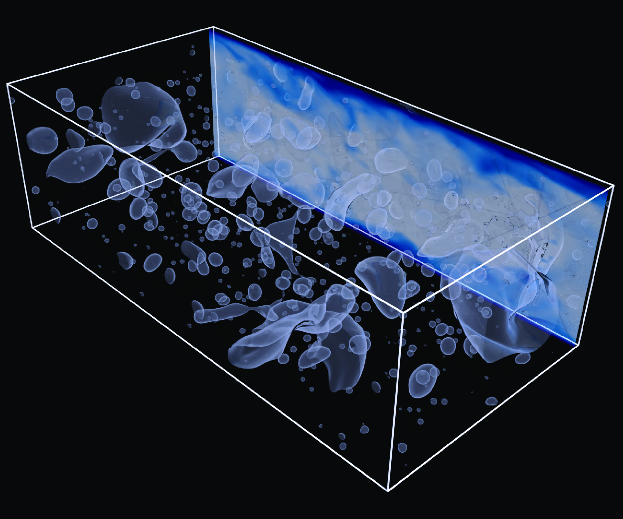
Figure 2. Instantaneous snapshots of bubbly upflow in a vertical channel. The density ratio is
 $\rho _l/\rho _g=1000$
, 30 and 10 for the top row, middle row and bottom row, respectively. The viscousity ratio is
$\rho _l/\rho _g=1000$
, 30 and 10 for the top row, middle row and bottom row, respectively. The viscousity ratio is
 $\mu _l / \mu _g = 100$
for all cases.
$\mu _l / \mu _g = 100$
for all cases.
We start the results analysis from the evolution of bubbles. Figure 2 presents instantaneous snapshots of bubbles for three cases. The top row shows the results for case R1000 with
 $\rho _l/\rho _g = 1000$
, which approximates a water–air system. Deformable bubbles aggregate in the core region, an observation qualitatively consistent with several previous studies at lower density ratios (Lu & Tryggvason Reference Lu and Tryggvason2008; Bolotnov et al. Reference Bolotnov, Jansen, Drew, Oberai, Lahey and Podowski2011; Dabiri et al. Reference Dabiri, Lu and Tryggvason2013; Du Cluzeau et al. Reference du Cluzeau, Bois and Toutant2019). Additionally, a large bubble forms in the core region, moving faster than the surrounding smaller bubbles. This large bubble continuously absorbs small bubbles and persists throughout the simulation duration. Similar bubble behaviour is also observed in the middle row for case R30 with
$\rho _l/\rho _g = 1000$
, which approximates a water–air system. Deformable bubbles aggregate in the core region, an observation qualitatively consistent with several previous studies at lower density ratios (Lu & Tryggvason Reference Lu and Tryggvason2008; Bolotnov et al. Reference Bolotnov, Jansen, Drew, Oberai, Lahey and Podowski2011; Dabiri et al. Reference Dabiri, Lu and Tryggvason2013; Du Cluzeau et al. Reference du Cluzeau, Bois and Toutant2019). Additionally, a large bubble forms in the core region, moving faster than the surrounding smaller bubbles. This large bubble continuously absorbs small bubbles and persists throughout the simulation duration. Similar bubble behaviour is also observed in the middle row for case R30 with
 $\rho _l/\rho _g = 30$
. However, such a large bubble is not seen in the bottom row, which shows the results for case R10 with the lowest density ratio
$\rho _l/\rho _g = 30$
. However, such a large bubble is not seen in the bottom row, which shows the results for case R10 with the lowest density ratio
 $\rho _l/\rho _g = 10$
under investigation. Instead, the size variation among bubbles is less significant in case R10 than in cases R30 and R1000, and the number of bubbles is smaller in case R10 than in cases R30 and R1000. The bubble distribution in case R10 is similar to the results reported by Lu & Tryggvason (Reference Lu and Tryggvason2018). A more detailed evolution process of bubbles is provided in the ementary movies.
$\rho _l/\rho _g = 10$
under investigation. Instead, the size variation among bubbles is less significant in case R10 than in cases R30 and R1000, and the number of bubbles is smaller in case R10 than in cases R30 and R1000. The bubble distribution in case R10 is similar to the results reported by Lu & Tryggvason (Reference Lu and Tryggvason2018). A more detailed evolution process of bubbles is provided in the ementary movies.

Figure 3. Evolution of bubble size for cases with density ratio (a)
 $\rho _l/\rho _g=10$
and (b)
$\rho _l/\rho _g=10$
and (b)
 $\rho _l/\rho _g=30$
. The contours represent the void fraction corresponding to the effective radius
$\rho _l/\rho _g=30$
. The contours represent the void fraction corresponding to the effective radius
 $\alpha _r$
(scales on the left vertical axis), normalised by the total void fraction of gas
$\alpha _r$
(scales on the left vertical axis), normalised by the total void fraction of gas
 $\alpha _t$
. The superimposed blue solid line denotes the total number of bubbles
$\alpha _t$
. The superimposed blue solid line denotes the total number of bubbles
 $N_b$
(scales on the right vertical axis).
$N_b$
(scales on the right vertical axis).
To visualise the evolution of bubbles with different sizes, we define an effective radius
 $r_e$
for each bubble based on its volume
$r_e$
for each bubble based on its volume
 $V_b$
as
$V_b$
as
 $r_e = (0.75V_b/\pi )^{1/3}$
. The volume of each bubble is determined using a connected component labelling algorithm (Herrmann Reference Herrmann2010). Figure 3 illustrates the evolution of bubble sizes for case R10N8 with
$r_e = (0.75V_b/\pi )^{1/3}$
. The volume of each bubble is determined using a connected component labelling algorithm (Herrmann Reference Herrmann2010). Figure 3 illustrates the evolution of bubble sizes for case R10N8 with
 $\rho _l/\rho _g = 10$
and case R30N8 with
$\rho _l/\rho _g = 10$
and case R30N8 with
 $\rho _l/\rho _g = 30$
. The contours represent the void fraction corresponding to the effective radius
$\rho _l/\rho _g = 30$
. The contours represent the void fraction corresponding to the effective radius
 $\alpha _r$
, normalised by the total void fraction of gas
$\alpha _r$
, normalised by the total void fraction of gas
 $\alpha _t$
. The evolution of the total number of bubbles,
$\alpha _t$
. The evolution of the total number of bubbles,
 $N_b$
, is superimposed as the solid line to demonstrate the convergence of the bubble number.
$N_b$
, is superimposed as the solid line to demonstrate the convergence of the bubble number.
The evolution of the total number of bubbles shown by the solid line in figure 3 converges at
 $t/t^* \approx 50$
. However, a longer time is needed for the bubbles with different sizes to evolve into a steady state. In these two cases, eight bubbles of equal diameter are initialised in the channel, and there is no change in their size during the early stages. After these initial bubbles break up into smaller ones around
$t/t^* \approx 50$
. However, a longer time is needed for the bubbles with different sizes to evolve into a steady state. In these two cases, eight bubbles of equal diameter are initialised in the channel, and there is no change in their size during the early stages. After these initial bubbles break up into smaller ones around
 $t/t^* \approx 12$
, bubbles with different sizes appear. For the low-density ratio case
$t/t^* \approx 12$
, bubbles with different sizes appear. For the low-density ratio case
 $\rho _l/\rho _g = 10$
(figure 3
a), bubbles first break into smaller ones with effective radii mainly ranging from
$\rho _l/\rho _g = 10$
(figure 3
a), bubbles first break into smaller ones with effective radii mainly ranging from
 $r_e/H = 0.1$
to
$r_e/H = 0.1$
to
 $0.3$
during
$0.3$
during
 $t/t^* = 12{-}30$
. Subsequently, smaller bubbles tend to merge into larger ones during
$t/t^* = 12{-}30$
. Subsequently, smaller bubbles tend to merge into larger ones during
 $t/t^* = 30{-}100$
, with the largest bubble reaching a size of
$t/t^* = 30{-}100$
, with the largest bubble reaching a size of
 $r_e/H \approx 0.55$
. The largest bubbles break into smaller ones during
$r_e/H \approx 0.55$
. The largest bubbles break into smaller ones during
 $t/t^* = 100{-}125$
, and after
$t/t^* = 100{-}125$
, and after
 $t/t^* = 125$
, the bubble size evolves to the statistically stationary state, with bubbles appearing across all scales from
$t/t^* = 125$
, the bubble size evolves to the statistically stationary state, with bubbles appearing across all scales from
 $r_e/H = 0.02$
to
$r_e/H = 0.02$
to
 $0.5$
. For the case with
$0.5$
. For the case with
 $\rho _l/\rho _g = 30$
(figure 3
b), the initial eight bubbles also start to break up into smaller ones after
$\rho _l/\rho _g = 30$
(figure 3
b), the initial eight bubbles also start to break up into smaller ones after
 $t/t^* \approx 12$
. Subsequently, the size of the largest bubble continuously increases during
$t/t^* \approx 12$
. Subsequently, the size of the largest bubble continuously increases during
 $t/t^{\ast} = 20 - 70$
. The size of the largest bubble reaches
$t/t^{\ast} = 20 - 70$
. The size of the largest bubble reaches
 $r_e/H \approx 0.65$
, and it persists for the entire simulation duration. By contrasting figures 3(a) and 3(b), it is seen that the number of smaller bubbles (with sizes ranging from
$r_e/H \approx 0.65$
, and it persists for the entire simulation duration. By contrasting figures 3(a) and 3(b), it is seen that the number of smaller bubbles (with sizes ranging from
 $r_e/H = 0.02$
to
$r_e/H = 0.02$
to
 $0.5$
) for
$0.5$
) for
 $\rho _l/\rho _g = 30$
is smaller than that for
$\rho _l/\rho _g = 30$
is smaller than that for
 $\rho _l/\rho _g = 10$
. A scale separation is evident in figure 3(b), where bubbles with
$\rho _l/\rho _g = 10$
. A scale separation is evident in figure 3(b), where bubbles with
 $ r_e/H \approx 0.4$
almost disappear.
$ r_e/H \approx 0.4$
almost disappear.

Figure 4. Bubble size spectra for cases with different density ratios. The two black solid lines indicate the
 $-3/2$
and
$-3/2$
and
 $-10/3$
power law proposed by Garrett et al. (Reference Garrett, Li and Farmer2000).
$-10/3$
power law proposed by Garrett et al. (Reference Garrett, Li and Farmer2000).
To further quantify the number of bubbles with different sizes, figure 4 shows the bubble size spectra for different cases after the bubbles evolve to a statistically stationary state. We note here that although the bubble size is sensitive to the initial condition at an early stage, the bubble statistics and turbulent statistics in the stationary steady-state are independent of the initial conditions (see Appendix B). Therefore, in the following content, the results for cases R1000, R100, R30 and R10 are analysed, while the results for cases R30N8 and R10N8 are not presented. It is seen from figure 4 that the bubbles at small scale show similar behaviour, while the number of large-scale bubbles is more sensitive to the density ratio. As the density ratio increases, the size of the largest bubble increases, whereas the number of bubbles with intermediate sizes between
 $0.07H$
and
$0.07H$
and
 $0.2H$
decreases. This decrease in the number of intermediate-sized bubbles occurs because these bubbles in the channel core region are absorbed by the largest bubble, as shown in figure 3(b) and the supplementary movies.
$0.2H$
decreases. This decrease in the number of intermediate-sized bubbles occurs because these bubbles in the channel core region are absorbed by the largest bubble, as shown in figure 3(b) and the supplementary movies.
The bubble size spectra are also compared with the power-law scaling proposed by Garrett et al. (Reference Garrett, Li and Farmer2000) for bubbles in the upper ocean in figure 4. A similar scaling law was also observed in a droplet-laden homogeneous isotropic turbulence (Cannon et al. Reference Cannon, Soligo and Rosti2024) and in a bubbly channel flow without gravity (Soligo et al. Reference Soligo, Roccon and Soldati2019). The result for
 $\rho _l / \rho _g = 10$
is consistent with the empirical law, but it deviates as the density ratio increases due to the combined effect of solid wall and gravity. In contrast to an upper ocean or a homogeneous condition, under which bubbles are free to cascade without the constraints of solid boundaries, bubbles are confined between two solid walls in the present study. The combined effect of gravity drives the bubbles to aggregate towards the channel core (Ervin & Tryggvason Reference Ervin and Tryggvason1997), ultimately resulting in the coalescence of smaller bubbles into larger ones. As the density ratio increases, the difference in the gravitational acceleration between gas and liquid increases, and as a result, the deviation of the bubble size spectra from the
$\rho _l / \rho _g = 10$
is consistent with the empirical law, but it deviates as the density ratio increases due to the combined effect of solid wall and gravity. In contrast to an upper ocean or a homogeneous condition, under which bubbles are free to cascade without the constraints of solid boundaries, bubbles are confined between two solid walls in the present study. The combined effect of gravity drives the bubbles to aggregate towards the channel core (Ervin & Tryggvason Reference Ervin and Tryggvason1997), ultimately resulting in the coalescence of smaller bubbles into larger ones. As the density ratio increases, the difference in the gravitational acceleration between gas and liquid increases, and as a result, the deviation of the bubble size spectra from the
 $-10/3$
law becomes more significant. More discussions about the effect of gravity on the bubble size are given in § 3.3 through a slip velocity between two phases (see figure 10 and corresponding discussions).
$-10/3$
law becomes more significant. More discussions about the effect of gravity on the bubble size are given in § 3.3 through a slip velocity between two phases (see figure 10 and corresponding discussions).
3.2. Turbulent statistics

Figure 5. Profiles of mean momentum
 $\langle \rho u \rangle$
in (a) wall units and (b) outer-layer units for single-phase turbulence and bubbly turbulence with different density ratios. The single-phase flow result of Tsukahara et al. (Reference Tsukahara, Seki, Kawamura and Tochio2005) is superimposed for validation.
$\langle \rho u \rangle$
in (a) wall units and (b) outer-layer units for single-phase turbulence and bubbly turbulence with different density ratios. The single-phase flow result of Tsukahara et al. (Reference Tsukahara, Seki, Kawamura and Tochio2005) is superimposed for validation.
Figure 5 compares the profiles of mean momentum
 $\left \langle \rho u \right \rangle$
for different density ratios. The angular brackets
$\left \langle \rho u \right \rangle$
for different density ratios. The angular brackets
 $\langle \ \rangle$
denote time and plane averaging as
$\langle \ \rangle$
denote time and plane averaging as
 \begin{align} \langle f \rangle (y) = \frac {1}{L_x L_z \Delta T} \int _0^{\Delta T} \int _{0}^{L_z} \int _{0}^{L_x} f(x, y, z, t) \mathrm {d}x \mathrm {d}z \mathrm {d}t , \end{align}
where
 $f$
represents an arbitrary variable and
$f$
represents an arbitrary variable and
 $\Delta T$
is the time duration of the data used for performing time averaging. Although the definition of averaging remains mathematically consistent with single-phase turbulent channel flow, what is analysed here is the mean momentum
$\Delta T$
is the time duration of the data used for performing time averaging. Although the definition of averaging remains mathematically consistent with single-phase turbulent channel flow, what is analysed here is the mean momentum
 $\langle \rho u \rangle$
. With the density involved in the averaging process, the mean momentum can be also regarded as a density-weighted mean velocity. This is different from single-phase turbulence. In two-phase flows, the momentum is a conservative quantity while the velocity is not. Therefore, comparing the mean momentum for different cases is more rational.
$\langle \rho u \rangle$
. With the density involved in the averaging process, the mean momentum can be also regarded as a density-weighted mean velocity. This is different from single-phase turbulence. In two-phase flows, the momentum is a conservative quantity while the velocity is not. Therefore, comparing the mean momentum for different cases is more rational.
In figure 5(a), the results are shown in wall units
 $y^+ = \rho _b y u_\tau / \mu _b$
, with the mean momentum non-dimensionalised using
$y^+ = \rho _b y u_\tau / \mu _b$
, with the mean momentum non-dimensionalised using
 $\rho _l u_\tau$
. The result for single-phase flow is compared with that of Tsukahara et al. (Reference Tsukahara, Seki, Kawamura and Tochio2005) for validation. The single-phase mean momentum agrees with the result in the literature. The mean momentum for single-phase flow aligns with the linear law in the viscous sub-layer and the logarithmic law in the outer layer. In bubbly flows, although the linear law still holds in the viscous sub-layer, the outer layer no longer conforms to the logarithmic law. As the density ratio increases from 10 to 30, the magnitude of
$\rho _l u_\tau$
. The result for single-phase flow is compared with that of Tsukahara et al. (Reference Tsukahara, Seki, Kawamura and Tochio2005) for validation. The single-phase mean momentum agrees with the result in the literature. The mean momentum for single-phase flow aligns with the linear law in the viscous sub-layer and the logarithmic law in the outer layer. In bubbly flows, although the linear law still holds in the viscous sub-layer, the outer layer no longer conforms to the logarithmic law. As the density ratio increases from 10 to 30, the magnitude of
 $\left \langle \rho u \right \rangle / \rho _l u_\tau$
continues to decrease in the core region. However, further increasing the density ratio from 30 to 1000 does not lead to significant changes in
$\left \langle \rho u \right \rangle / \rho _l u_\tau$
continues to decrease in the core region. However, further increasing the density ratio from 30 to 1000 does not lead to significant changes in
 $\left \langle \rho u \right \rangle / \rho _l u_\tau$
. The effect of density ratio on the mean momentum can be equivalently shown using an outer-layer scaling (figure 5
b), with the bulk mean velocity
$\left \langle \rho u \right \rangle / \rho _l u_\tau$
. The effect of density ratio on the mean momentum can be equivalently shown using an outer-layer scaling (figure 5
b), with the bulk mean velocity
 $u_b=M_b/\rho _b$
and half-width of channel
$u_b=M_b/\rho _b$
and half-width of channel
 $H$
being the characteristic velocity and length scales, respectively. The gradient of mean momentum is steeper in bubbly flows in the near-wall region. The velocity gradient further increases as the density ratio increases from
$H$
being the characteristic velocity and length scales, respectively. The gradient of mean momentum is steeper in bubbly flows in the near-wall region. The velocity gradient further increases as the density ratio increases from
 $\rho _l / \rho _g = 10$
to 30. The profiles of
$\rho _l / \rho _g = 10$
to 30. The profiles of
 $\left \langle \rho u \right \rangle / \rho _l u_b$
for
$\left \langle \rho u \right \rangle / \rho _l u_b$
for
 $\rho _l / \rho _g = 30$
, 100 and 1000 collapse, indicating a saturated effect of density ratio on the mean momentum for higher density ratios. We also examined the effect of viscosity ratio on the turbulent statistics. The viscosity ratio effect is less significant than the density ratio effect (see Appendix C). Therefore, the following analyses focus on the effects of the density ratio.
$\rho _l / \rho _g = 30$
, 100 and 1000 collapse, indicating a saturated effect of density ratio on the mean momentum for higher density ratios. We also examined the effect of viscosity ratio on the turbulent statistics. The viscosity ratio effect is less significant than the density ratio effect (see Appendix C). Therefore, the following analyses focus on the effects of the density ratio.
To further explore the momentum transfer in bubbly turbulence, we integrated the mean momentum equation from the bottom wall to an arbitrary wall-normal coordinate
 $y$
to yield the following balance equation of the mean shear stress:
$y$
to yield the following balance equation of the mean shear stress:
 \begin{align} \Pi y = \underbrace {\left \langle \mu \left (\frac {\partial u}{\partial y } + \frac {\partial v}{\partial x}\right )\right \rangle }_{{S}} \underbrace {-\left \langle \rho u'v' \right \rangle }_{{C}} \underbrace {-\int _{-H}^{y}{\left \langle \rho -{{\rho }_{b}} \right \rangle g{\textrm{d}}y}}_{ {G}}+\underbrace {\int _{-H}^{y}{\left \langle {\sigma \kappa \frac {\partial H(\phi )}{\partial {x}}} \right \rangle {\textrm{d}}y}}_{ {T}} . \end{align}
On the right-hand side, S, C, G and T represent the shear stresses corresponding to the viscosity, convection, gravity and surface tension, respectively. The convection shear stress C is also known as Reynolds shear stress in single-phase turbulence. On the left-hand side, the total shear stress
 $\Pi y$
shows a straight line with a slope of
$\Pi y$
shows a straight line with a slope of
 $\Pi$
. Figure 6 compares the profiles of the mean stresses between single-phase turbulence and bubbly turbulence with
$\Pi$
. Figure 6 compares the profiles of the mean stresses between single-phase turbulence and bubbly turbulence with
 $\rho _l / \rho _g = 1000$
. In the single-phase flow (figure 6
a), the total shear stress is dominated by the viscosity shear stress
$\rho _l / \rho _g = 1000$
. In the single-phase flow (figure 6
a), the total shear stress is dominated by the viscosity shear stress
 $S$
and Reynolds stress
$S$
and Reynolds stress
 $C$
in the near-wall and core regions, respectively. In the bubbly flow, as shown in figure 6(b), the viscous stress still dominates the near-wall region. In the core region, the gravity term
$C$
in the near-wall and core regions, respectively. In the bubbly flow, as shown in figure 6(b), the viscous stress still dominates the near-wall region. In the core region, the gravity term
 $G$
exhibits an opposite sign to the total shear stress
$G$
exhibits an opposite sign to the total shear stress
 $\Pi y$
. Compared with the single-phase turbulence, the magnitude of the convection shear stress
$\Pi y$
. Compared with the single-phase turbulence, the magnitude of the convection shear stress
 $C$
is larger in bubbly turbulence, with its peak shifting towards the core region, to balance the negative effect of
$C$
is larger in bubbly turbulence, with its peak shifting towards the core region, to balance the negative effect of
 $G$
. The surface tension term
$G$
. The surface tension term
 $T$
provides shear stress when bubbles are stretched in the shear direction (Lu & Tryggvason Reference Lu and Tryggvason2019; Du Cluzeau et al. Reference du Cluzeau, Bois and Toutant2019; Cannon et al. Reference Cannon, Izbassarov, Tammisola, Brandt and Rosti2021; Lee et al. Reference Lee, Chang, Kim and Choi2024). In the present cases, it is small compared with other terms.
$T$
provides shear stress when bubbles are stretched in the shear direction (Lu & Tryggvason Reference Lu and Tryggvason2019; Du Cluzeau et al. Reference du Cluzeau, Bois and Toutant2019; Cannon et al. Reference Cannon, Izbassarov, Tammisola, Brandt and Rosti2021; Lee et al. Reference Lee, Chang, Kim and Choi2024). In the present cases, it is small compared with other terms.

Figure 6. Balance of mean shear stress given by (3.2) for (a) single-phase turbulence and (b) bubbly turbulence with
 $\rho _l/\rho _g = 1000$
. All terms are non-dimensionalised using
$\rho _l/\rho _g = 1000$
. All terms are non-dimensionalised using
 $\rho _bu^2_b$
.
$\rho _bu^2_b$
.
In single-phase turbulence, the well-known FIK identity (Fukagata, Iwamoto & Kasagi Reference Fukagata, Iwamoto and Kasagi2002) links the wall friction to the turbulent motion. To investigate the contributions of the different components of the mean shear stress in (3.2) to the wall friction in bubbly turbulence, we derive the following generalised form of the FIK identity in a bubbly channel flow:
 \begin{align} \int _{-H}^{0}{yC^{{eff}}{\textrm{d}}y}+\int _{-H}^{0}{y\left \langle \mu \left (\frac {\partial u}{\partial y } + \frac {\partial v}{\partial x}\right )\right \rangle {\textrm{d}}y}=\int _{-H}^{0}{\Pi y^2{\textrm{d}}y}=\frac {\tau _wH^2}{3}, \end{align}
where
 $C^{{eff}}=G+C+T$
denotes a defined effective Reynolds stress to maintain the form consistent with the original FIK identity, and
$C^{{eff}}=G+C+T$
denotes a defined effective Reynolds stress to maintain the form consistent with the original FIK identity, and
 $\tau _w = \Pi H$
denotes the wall shear stress. The skin friction coefficient
$\tau _w = \Pi H$
denotes the wall shear stress. The skin friction coefficient
 $C_f$
is then decomposed as follows:
$C_f$
is then decomposed as follows:
 \begin{align} C_f=\frac {2\tau _w}{\rho u^2_b}=\underbrace {\frac {6}{\rho u^2_bH^2}\int _{-H}^{0}{yC^{{eff}}{\textrm{d}}y}}_{C^T_f}+\underbrace {\frac {6}{\rho u^2_bH^2}\int _{-H}^{0}{y\left \langle \mu \left (\frac {\partial u}{\partial y } + \frac {\partial v}{\partial x}\right )\right \rangle {\textrm{d}}y}}_{C^L_f}, \end{align}
where
 $C^T_f$
and
$C^T_f$
and
 $C^L_f$
represent the turbulent and laminar contributions, respectively, to the total wall friction coefficient
$C^L_f$
represent the turbulent and laminar contributions, respectively, to the total wall friction coefficient
 $C_f$
. For single-phase turbulent channel flows, the laminar part
$C_f$
. For single-phase turbulent channel flows, the laminar part
 $C^L_f=6\mu /\rho u_bH=6/Re_b$
, with
$C^L_f=6\mu /\rho u_bH=6/Re_b$
, with
 $Re_b=\rho _bu_bH/\mu _b$
, can be obtained analytically. In bubbly flows, analytical integration is not feasible since
$Re_b=\rho _bu_bH/\mu _b$
, can be obtained analytically. In bubbly flows, analytical integration is not feasible since
 $\mu$
varies with local flow conditions. Consequently, we performed numerical integration of this term using simulation data. Figure 7 illustrates the laminar and turbulent contributions to the total wall friction coefficient. For comparison, the decomposed wall friction coefficients
$\mu$
varies with local flow conditions. Consequently, we performed numerical integration of this term using simulation data. Figure 7 illustrates the laminar and turbulent contributions to the total wall friction coefficient. For comparison, the decomposed wall friction coefficients
 $C^T_f$
and
$C^T_f$
and
 $C^L_f$
were normalised using the analytical laminar value,
$C^L_f$
were normalised using the analytical laminar value,
 $6/Re_b$
. The presence of bubbles does not alter the laminar part of
$6/Re_b$
. The presence of bubbles does not alter the laminar part of
 $C^L_f$
, whereas the turbulent part of
$C^L_f$
, whereas the turbulent part of
 $C^T_f$
is higher in bubbly flows than in single-phase flows. The friction Reynolds number
$C^T_f$
is higher in bubbly flows than in single-phase flows. The friction Reynolds number
 $Re_\tau$
for all cases is superimposed in figure 7, and it can be observed that
$Re_\tau$
for all cases is superimposed in figure 7, and it can be observed that
 $Re_\tau$
follows the behaviour of
$Re_\tau$
follows the behaviour of
 $C^T_f$
as the density ratio increases. Specifically, both
$C^T_f$
as the density ratio increases. Specifically, both
 $Re_\tau$
and
$Re_\tau$
and
 $C^T_f$
were larger in bubbly turbulence than in single-phase turbulence, whereas as the density ratio increased from 10 to 30, both increased further. The increase in
$C^T_f$
were larger in bubbly turbulence than in single-phase turbulence, whereas as the density ratio increased from 10 to 30, both increased further. The increase in
 $Re_\tau$
and
$Re_\tau$
and
 $C^T_f$
slowed down as the density ratio further increased from 30 to 1000, which is consistent with the observations in figure 5 for the saturation of the mean momentum. The above observation suggests that the inclusion of bubbles induces additional drag compared with a single-phase flow.
$C^T_f$
slowed down as the density ratio further increased from 30 to 1000, which is consistent with the observations in figure 5 for the saturation of the mean momentum. The above observation suggests that the inclusion of bubbles induces additional drag compared with a single-phase flow.

Figure 7. Contributions of laminar (
 $C^L_f$
, triangles) and turbulent (
$C^L_f$
, triangles) and turbulent (
 $C^T_f$
, circles) parts to the total wall friction coefficient (
$C^T_f$
, circles) parts to the total wall friction coefficient (
 $C_f$
) in cases with different density ratios (scales on the left
$C_f$
) in cases with different density ratios (scales on the left
 $y$
-axis). Both
$y$
-axis). Both
 $C^L_f$
and
$C^L_f$
and
 $C^T_f$
are normalised using the laminar contribution
$C^T_f$
are normalised using the laminar contribution
 $6/Re_b$
for single-phase flow. The diamond shows the friction Reynolds number in different cases (scales on the right
$6/Re_b$
for single-phase flow. The diamond shows the friction Reynolds number in different cases (scales on the right
 $y$
-axis). Solid and hollow symbols represent single-phase and bubble flows, respectively.
$y$
-axis). Solid and hollow symbols represent single-phase and bubble flows, respectively.

Figure 8. Profiles of (a) Reynolds stress
 $C$
, (b) effective Reynolds stress
$C$
, (b) effective Reynolds stress
 $C^{{eff}}\!,$
(c) bubble internal force
$C^{{eff}}\!,$
(c) bubble internal force
 $B$
and (d) averaged bubble void fraction
$B$
and (d) averaged bubble void fraction
 $\langle \alpha \rangle$
for single-phase turbulence and bubbly turbulence with different density ratios.
$\langle \alpha \rangle$
for single-phase turbulence and bubbly turbulence with different density ratios.
The results shown in figure 7 suggest that the effect of density ratio on the wall friction is primarily determined by the effective Reynolds stress
 $C^{{eff}}$
. This reminds us to decompose the convection term
$C^{{eff}}$
. This reminds us to decompose the convection term
 $C$
into two parts in the bubbly turbulence to examine the effect of density ratio separately. One part is
$C$
into two parts in the bubbly turbulence to examine the effect of density ratio separately. One part is
 $B=-(G+T)$
that balances the internal forces exerted by the bubbles, including the effects of gravity (
$B=-(G+T)$
that balances the internal forces exerted by the bubbles, including the effects of gravity (
 $G$
) and surface tension (
$G$
) and surface tension (
 $T$
). This component has no net contribution to wall friction. The other part is the effective Reynolds stress
$T$
). This component has no net contribution to wall friction. The other part is the effective Reynolds stress
 $C^{{eff}}$
that influences the wall friction.
$C^{{eff}}$
that influences the wall friction.
Figure 8 compares the profiles of
 $C$
,
$C$
,
 $C^{{eff}}$
,
$C^{{eff}}$
,
 $B$
and bubble void fraction
$B$
and bubble void fraction
 $\langle \alpha \rangle$
for various density ratios. As shown in figure 8(a), the magnitude of
$\langle \alpha \rangle$
for various density ratios. As shown in figure 8(a), the magnitude of
 $C$
increases as the density ratio increases from 10 to 30, while the difference of
$C$
increases as the density ratio increases from 10 to 30, while the difference of
 $C$
between R30 an R1000 is less significant. Figure 8(b) shows that the peak of the effective Reynolds stress
$C$
between R30 an R1000 is less significant. Figure 8(b) shows that the peak of the effective Reynolds stress
 $C^{{eff}}$
is located in the near-wall region for all cases. As the density ratio increases, the magnitude of this peak increases, with its location shifting towards the wall. This observation indicates that the bubbles influence the wall friction by altering the near-wall structures. Figure 8(c) shows that
$C^{{eff}}$
is located in the near-wall region for all cases. As the density ratio increases, the magnitude of this peak increases, with its location shifting towards the wall. This observation indicates that the bubbles influence the wall friction by altering the near-wall structures. Figure 8(c) shows that
 $B$
is trivial in a single-phase flow. The significant increase in the magnitude of
$B$
is trivial in a single-phase flow. The significant increase in the magnitude of
 $C$
with the inclusion of bubbles is primarily caused by the bubble internal force component,
$C$
with the inclusion of bubbles is primarily caused by the bubble internal force component,
 $B$
. The peak of
$B$
. The peak of
 $B$
is located at approximately
$B$
is located at approximately
 $y/H = -0.5$
, resulting in the shift of the convective shear stress,
$y/H = -0.5$
, resulting in the shift of the convective shear stress,
 $C$
, towards the channel centre. The bubble internal forces are also closely related to the mean gas void fraction. Figure 8(d) presents the vertical profiles of the averaged bubble void fraction,
$C$
, towards the channel centre. The bubble internal forces are also closely related to the mean gas void fraction. Figure 8(d) presents the vertical profiles of the averaged bubble void fraction,
 $\langle \alpha \rangle$
, for different cases, with the horizontal dash-dotted line representing bulk void fraction
$\langle \alpha \rangle$
, for different cases, with the horizontal dash-dotted line representing bulk void fraction
 $\alpha _t$
. The intersection points between this horizontal line and the profiles of
$\alpha _t$
. The intersection points between this horizontal line and the profiles of
 $\langle \alpha \rangle$
is close to the peak locations of
$\langle \alpha \rangle$
is close to the peak locations of
 $B$
in figure 8(c) for all cases. The greater number of deformable bubbles with sizes
$B$
in figure 8(c) for all cases. The greater number of deformable bubbles with sizes
 $r_e/H = 0.1\sim 0.4$
(figure 4) in the case with
$r_e/H = 0.1\sim 0.4$
(figure 4) in the case with
 $\rho _l/\rho _g = 10$
results in a larger proportion of gas being distributed in the channel core region (
$\rho _l/\rho _g = 10$
results in a larger proportion of gas being distributed in the channel core region (
 $y/H \geqslant - 0.75$
). Consequently, the peak position of
$y/H \geqslant - 0.75$
). Consequently, the peak position of
 $B$
for
$B$
for
 $\rho _l/\rho _g = 10$
is closer to the core region than that for other cases. Another notable observation is that
$\rho _l/\rho _g = 10$
is closer to the core region than that for other cases. Another notable observation is that
 $\langle \alpha \rangle$
is larger near
$\langle \alpha \rangle$
is larger near
 $y/H = -0.5$
in cases with higher density ratios compared with the lowest density ratio case. This is because the dominant large bubble is substantial in size and extends to the
$y/H = -0.5$
in cases with higher density ratios compared with the lowest density ratio case. This is because the dominant large bubble is substantial in size and extends to the
 $y/H = -0.5$
region, resulting in a higher void fraction at this location. These observations suggest that while the internal forces do not directly contribute to wall friction, they significantly influence the flow dynamics in the core region.
$y/H = -0.5$
region, resulting in a higher void fraction at this location. These observations suggest that while the internal forces do not directly contribute to wall friction, they significantly influence the flow dynamics in the core region.
3.3. Interaction between turbulence and bubbles

Figure 9. Instantaneous snapshots of the bubbles and vortex structures coloured by
 $u$
. The vortex structures are shown using the isosurface of Q = 1 and Q = 10 for single-phase and bubbly flow cases, respectively. The upper and lower rows show the vortex structures conditioned by
$u$
. The vortex structures are shown using the isosurface of Q = 1 and Q = 10 for single-phase and bubbly flow cases, respectively. The upper and lower rows show the vortex structures conditioned by
 $u\lt u_b$
and
$u\lt u_b$
and
 $u\gt u_b$
, respectively. Each column shows the results for one case: (a, b) single-phase flow, (c, d)
$u\gt u_b$
, respectively. Each column shows the results for one case: (a, b) single-phase flow, (c, d)
 $\rho _l / \rho _g = 10$
, (e, f)
$\rho _l / \rho _g = 10$
, (e, f)
 $\rho _l / \rho _g = 30$
, (g, h)
$\rho _l / \rho _g = 30$
, (g, h)
 $\rho _l / \rho _g = 100$
and (i, j)
$\rho _l / \rho _g = 100$
and (i, j)
 $\rho _l / \rho _g = 1000$
.
$\rho _l / \rho _g = 1000$
.
From the above analysis, the influence of the density ratio on the flow dynamics differs between the near-wall and core regions. In this section, we further analyse the influences of turbulence and bubbles on each other. Figure 9 compares instantaneous snapshots of the vortex structures and bubbles in different cases. Because the streamwise velocity
 $u$
is in general larger in the core region than in the near-wall region, its value is used as a condition to distinguish the vortex structures in different regions. Specifically, in the upper and lower rows of figure 9, vortex structures with
$u$
is in general larger in the core region than in the near-wall region, its value is used as a condition to distinguish the vortex structures in different regions. Specifically, in the upper and lower rows of figure 9, vortex structures with
 $u\lt u_b$
and
$u\lt u_b$
and
 $u\gt u_b$
are shown. Therefore, vortex structures in the near-wall and core regions are observed in the upper and lower rows, respectively.
$u\gt u_b$
are shown. Therefore, vortex structures in the near-wall and core regions are observed in the upper and lower rows, respectively.
The upper row in figure 9 shows that small bubbles dominate the near-wall region. The vortex structures are broken into smaller structures by these small bubbles (figures 9
c, 9
e, 9
g and 9
i). This effect enhances the wall-normal fluctuation in the near-wall region, leading to an increase in the wall friction. The distribution of small bubbles in the near-wall region remains similar for cases with
 $\rho _l/\rho _g \geqslant 30$
, such that the wall friction saturates for higher density ratios.
$\rho _l/\rho _g \geqslant 30$
, such that the wall friction saturates for higher density ratios.
In the core region, large bubbles tend to generate vortex structures in their wakes (figures 9 d, 9 f, 9 h and 9 j), and the sizes of these large bubbles increases with an increasing density ratio. Furthermore, more vortex structures are observed in the wake of large bubbles in the cases with higher density ratios. Several small bubbles are trapped in the wake regions of the large bubbles. These small bubbles are continuously absorbed by larger bubbles, increasing the size of the large bubble (figures 9 f, 9 h and 9 j).

Figure 10. Profiles of (a) mean velocity in the gas phase
 $\langle u \rangle _g$
, (b) mean velocity in the liquid phase
$\langle u \rangle _g$
, (b) mean velocity in the liquid phase
 $\langle u \rangle _l$
and (c) slip velocity
$\langle u \rangle _l$
and (c) slip velocity
 $\langle u \rangle _s = \langle u \rangle _g - \langle u \rangle _l$
for bubbly turbulence with different density ratios.
$\langle u \rangle _s = \langle u \rangle _g - \langle u \rangle _l$
for bubbly turbulence with different density ratios.
The vortex structures in the wake region of large bubbles are attributed to the slip velocity between the liquid and gas phases. Figure 10 shows a comparison of the mean velocities of the gas phase
 $\langle u \rangle _g$
, liquid phase
$\langle u \rangle _g$
, liquid phase
 $\langle u \rangle _l$
and the slip velocity
$\langle u \rangle _l$
and the slip velocity
 $\langle u \rangle _s = \langle u \rangle _g - \langle u \rangle _l$
for various density ratios. As shown in figure 10(a), owing to the stronger buoyancy effect, the mean velocity of the gas phase is higher for the case with a larger density ratio. Meanwhile, the change in liquid velocity is insignificant (figure 10
b), resulting in a higher slip velocity between the two phases in cases with higher density ratios (figure 10
c). The relative motion between bubbles and the surrounding liquid generates vortex structures in the wake of the large bubble, and more vortex structures are observed in the wake of bubbles with an increasing density ratio (figures 9
c, 9
e, 9
g and 9
i) because of the larger slip velocity (figure 10
c). However, as observed in figures 5 and 8, the differences in mean momentum
$\langle u \rangle _s = \langle u \rangle _g - \langle u \rangle _l$
for various density ratios. As shown in figure 10(a), owing to the stronger buoyancy effect, the mean velocity of the gas phase is higher for the case with a larger density ratio. Meanwhile, the change in liquid velocity is insignificant (figure 10
b), resulting in a higher slip velocity between the two phases in cases with higher density ratios (figure 10
c). The relative motion between bubbles and the surrounding liquid generates vortex structures in the wake of the large bubble, and more vortex structures are observed in the wake of bubbles with an increasing density ratio (figures 9
c, 9
e, 9
g and 9
i) because of the larger slip velocity (figure 10
c). However, as observed in figures 5 and 8, the differences in mean momentum
 $\langle \rho u \rangle$
and Reynolds shear stress
$\langle \rho u \rangle$
and Reynolds shear stress
 $-\langle \rho u' v'\rangle$
are insignificant for density ratios larger than 30. This further confirms that the wall friction is mainly influenced by the near-wall structures.
$-\langle \rho u' v'\rangle$
are insignificant for density ratios larger than 30. This further confirms that the wall friction is mainly influenced by the near-wall structures.

Figure 11. Profiles of (a)
 $u_{\mathrm {rms}}$
, (b)
$u_{\mathrm {rms}}$
, (b)
 $v_{\mathrm {rms}}$
and the density-weighted correlation coefficient
$v_{\mathrm {rms}}$
and the density-weighted correlation coefficient
 $R_{uv}$
between streamwise and wall-normal velocity fluctuations for single-phase turbulence and bubbly turbulence with different density ratios. .
$R_{uv}$
between streamwise and wall-normal velocity fluctuations for single-phase turbulence and bubbly turbulence with different density ratios. .
This analysis of the slip velocity explains the observation in figure 9 that the vortex structures in the core region are increasingly intensified for a higher density ratio. To quantitatively demonstrate the contribution of wake vortices, we examined the density weighted root-mean-square velocities
 $u_{\mathrm {rms}} = (\langle \rho u^\prime u^\prime \rangle / \rho _b )^{1/2}$
and
$u_{\mathrm {rms}} = (\langle \rho u^\prime u^\prime \rangle / \rho _b )^{1/2}$
and
 $ v_{\mathrm {rms}} = ( \langle \rho v^\prime v^\prime \rangle / \rho _b )^{1/2}$
, and
$ v_{\mathrm {rms}} = ( \langle \rho v^\prime v^\prime \rangle / \rho _b )^{1/2}$
, and
 $R_{uv} = -\langle \rho u^\prime v^\prime \rangle / (\rho _b u_{\mathrm {rms}} v_{\mathrm {rms}} )$
, the correlation coefficient between
$R_{uv} = -\langle \rho u^\prime v^\prime \rangle / (\rho _b u_{\mathrm {rms}} v_{\mathrm {rms}} )$
, the correlation coefficient between
 $u'$
and
$u'$
and
 $v'$
. We weighted the correlation coefficient by density because
$v'$
. We weighted the correlation coefficient by density because
 $-\langle \rho u^\prime v^\prime \rangle$
appears as the Reynolds shear stress in the balance equation (3.2) of the mean momentum
$-\langle \rho u^\prime v^\prime \rangle$
appears as the Reynolds shear stress in the balance equation (3.2) of the mean momentum
 $\langle \rho u \rangle$
for two-fluid flow rather than
$\langle \rho u \rangle$
for two-fluid flow rather than
 $-\langle u^\prime v^\prime \rangle$
in single-phase flow. The results of
$-\langle u^\prime v^\prime \rangle$
in single-phase flow. The results of
 $u_{\mathrm {rms}}$
,
$u_{\mathrm {rms}}$
,
 $v_{\mathrm {rms}}$
and
$v_{\mathrm {rms}}$
and
 $R_{uv}$
for various density ratios are shown in figure 11. From these figures, dual effects of wake vortices on the Reynolds shear stress are observed. On the one hand, the occurrence of wake vortices enhances the velocity fluctuations in both the streamwise and vertical directions. Specifically, the magnitudes of both
$R_{uv}$
for various density ratios are shown in figure 11. From these figures, dual effects of wake vortices on the Reynolds shear stress are observed. On the one hand, the occurrence of wake vortices enhances the velocity fluctuations in both the streamwise and vertical directions. Specifically, the magnitudes of both
 $u_{\mathrm {rms}}$
and
$u_{\mathrm {rms}}$
and
 $v_{\mathrm {rms}}$
increase monotonically as the density ratio increases, with larger values occurring in the channel core for higher density ratio cases. This observation suggests that at higher density ratios, the stronger vortex structures (as shown in figure 9) in the wakes of large bubbles are responsible for intensifying velocity fluctuations in the core region. On the other hand, the magnitude of
$v_{\mathrm {rms}}$
increase monotonically as the density ratio increases, with larger values occurring in the channel core for higher density ratio cases. This observation suggests that at higher density ratios, the stronger vortex structures (as shown in figure 9) in the wakes of large bubbles are responsible for intensifying velocity fluctuations in the core region. On the other hand, the magnitude of
 $R_{uv}$
decreases monotonically as the density ratio increases. This indicates that the wake vortices also impose a decorrelation effect on the streamwise and wall-normal velocity fluctuations. The Reynolds stress can be also written as
$R_{uv}$
decreases monotonically as the density ratio increases. This indicates that the wake vortices also impose a decorrelation effect on the streamwise and wall-normal velocity fluctuations. The Reynolds stress can be also written as
 $-\langle \rho u^\prime v^\prime \rangle = \rho _b R_{uv} u_{\mathrm {rms}} v_{\mathrm {rms}}$
. The enhancement effects of wake vortices on
$-\langle \rho u^\prime v^\prime \rangle = \rho _b R_{uv} u_{\mathrm {rms}} v_{\mathrm {rms}}$
. The enhancement effects of wake vortices on
 $u_{\mathrm {rms}}$
and
$u_{\mathrm {rms}}$
and
 $v_{\mathrm {rms}}$
are balanced by their suppression effect on
$v_{\mathrm {rms}}$
are balanced by their suppression effect on
 $R_{uv}$
. Consequently, the Reynolds stress remains almost unchanged for cases with different density ratios in the core region.
$R_{uv}$
. Consequently, the Reynolds stress remains almost unchanged for cases with different density ratios in the core region.

Figure 12. Profiles of Reynolds stresses
 $-\langle \rho u'v'\rangle$
conditioned by (a) Q1, (b) Q2, (c) Q3 and (d) Q4 events.
$-\langle \rho u'v'\rangle$
conditioned by (a) Q1, (b) Q2, (c) Q3 and (d) Q4 events.
To further investigate the mechanism underlying the saturation of wall friction for
 $\rho _l / \rho _g \geqslant 30$
, and the decorrelation effect of wake vortices on
$\rho _l / \rho _g \geqslant 30$
, and the decorrelation effect of wake vortices on
 $u'$
and
$u'$
and
 $v'$
in the core region, we performed a quadrant analysis of the Reynolds stress. Figure 12 depicts the Reynolds stress conditioned by the signs of
$v'$
in the core region, we performed a quadrant analysis of the Reynolds stress. Figure 12 depicts the Reynolds stress conditioned by the signs of
 $u'$
and
$u'$
and
 $v'$
. Four quadrants, Q1–Q4, denote the conditions
$v'$
. Four quadrants, Q1–Q4, denote the conditions
 $(u'\gt 0, v'\gt 0)$
,
$(u'\gt 0, v'\gt 0)$
,
 $(u'\lt 0, v'\gt 0)$
,
$(u'\lt 0, v'\gt 0)$
,
 $(u'\lt 0, v'\lt 0)$
and
$(u'\lt 0, v'\lt 0)$
and
 $(u'\gt 0, v'\lt 0)$
, respectively. It is observed that Reynolds stresses corresponding to all four quadrants are larger in bubbly turbulence than in the single-phase turbulence. This indicates that the wall-normal motion and corresponding momentum convection are more active in a bubbly channel. In the near-wall region (
$(u'\gt 0, v'\lt 0)$
, respectively. It is observed that Reynolds stresses corresponding to all four quadrants are larger in bubbly turbulence than in the single-phase turbulence. This indicates that the wall-normal motion and corresponding momentum convection are more active in a bubbly channel. In the near-wall region (
 $y/H \leqslant -0.9$
), as the density ratio increases from 10 to 30, the increase in Q2 and Q4 events is more significant, leading to the overall increase in
$y/H \leqslant -0.9$
), as the density ratio increases from 10 to 30, the increase in Q2 and Q4 events is more significant, leading to the overall increase in
 $C^{{eff}}$
and leading to a higher wall friction. Additionally, in the near-wall region, the contributions of Q1–Q4 to the total Reynolds stress all saturate for
$C^{{eff}}$
and leading to a higher wall friction. Additionally, in the near-wall region, the contributions of Q1–Q4 to the total Reynolds stress all saturate for
 $\rho _l/\rho _g \geqslant 30$
, resulting in the saturation of effective Reynolds stress and wall friction. In the core region (
$\rho _l/\rho _g \geqslant 30$
, resulting in the saturation of effective Reynolds stress and wall friction. In the core region (
 $y/H \geqslant -0.5$
), an increase in the contribution of Q1 and Q3 events is comparable to that of Q2 and Q4 events. This results in a negligible net contribution to the total Reynolds stress, as shown in figure 8(a).
$y/H \geqslant -0.5$
), an increase in the contribution of Q1 and Q3 events is comparable to that of Q2 and Q4 events. This results in a negligible net contribution to the total Reynolds stress, as shown in figure 8(a).
It is worth noting that the suppression of turbulence in bubbly upflow mentioned by Takagi & Matsumoto (Reference Takagi and Matsumoto2011) is not observed in the present study. The experimental results of So et al. (Reference So, Morikita, Takagi and Matsumoto2002) indicate that adding a certain amount of surfactant to the liquid can prevent the coalescence of bubbles into larger ones, resulting in bubbles with a diameter of approximately 1 mm occupying the channel. Due to shear-induced lateral forces, bubbles accumulate near the wall, forming a sheet-like structure that pulls the surrounding liquid upward through buoyancy. The buoyant bubble sheet typically spans a few hundred wall units in a turbulent boundary layer, creating two distinct regions with different velocity fluctuation behaviours. In the narrow region between the wall and the bubble sheet, fluctuations are primarily generated by high-shear-rate turbulence. In the outer region, fluctuations are caused by the motion of bubbles rising in a plug-like flow, with significantly suppressed velocity fluctuations compared with single-phase turbulence.
However, a bubble sheet is not observed in the present study, even though the flow parameters for case R1000 with
 $\rho _l / \rho _g = 1000$
are close to those of the experimental set-up. This discrepancy is presumably because there are no surfactants in the present simulations, as such bubbles coalesce to form larger bubbles. The wakes of larger bubbles interact with the wall layer, preventing smaller bubbles (with
$\rho _l / \rho _g = 1000$
are close to those of the experimental set-up. This discrepancy is presumably because there are no surfactants in the present simulations, as such bubbles coalesce to form larger bubbles. The wakes of larger bubbles interact with the wall layer, preventing smaller bubbles (with
 $r_e/H = 0.025$
, corresponding to 1-mm bubbles in the experiment) from forming a bubble sheet. Consequently, large buoyancy effects near the wall are not observed. Furthermore, as noted by Takagi & Matsumoto (Reference Takagi and Matsumoto2011), the tangential stress at the gas–liquid interface resulting from the Marangoni effect becomes non-negligible when surfactants are added. Bubble clustering is observed only when a specific amount of surfactants is added; otherwise, the bubbles are uniformly dispersed across the channel. This could also be another important factor that no bubble sheet is formed in the present simulations.
$r_e/H = 0.025$
, corresponding to 1-mm bubbles in the experiment) from forming a bubble sheet. Consequently, large buoyancy effects near the wall are not observed. Furthermore, as noted by Takagi & Matsumoto (Reference Takagi and Matsumoto2011), the tangential stress at the gas–liquid interface resulting from the Marangoni effect becomes non-negligible when surfactants are added. Bubble clustering is observed only when a specific amount of surfactants is added; otherwise, the bubbles are uniformly dispersed across the channel. This could also be another important factor that no bubble sheet is formed in the present simulations.
The above discussion on the difference between the present study and the experiments of So et al. (Reference So, Morikita, Takagi and Matsumoto2002) is also supported by several previous numerical studies. By preventing bubble coalescence, Lu & Tryggvason (Reference Lu and Tryggvason2013) observed the occurrence of bubble sheets near the wall and the suppression of velocity fluctuations. However, the suppression disappears when bubbles are allowed to coalesce, as shown in a later study of Lu & Tryggvason (Reference Lu and Tryggvason2019). They also showed that the wakes of larger bubbles in the channel core can disturb the wall layer, even at a relatively low density ratio of 10. Thus, it is reasonable that the bubble sheet is absent in our study.
4. Conclusions
In this study, phase-resolved simulations were performed to investigate the effect of the density ratio on turbulent statistics and vortex structures in a bubbly channel flow. The main objective is to determine whether a relatively low density ratio exists at which the turbulent statistics are representative of a real air–water system with a high density ratio close to 1000. The primary discovery of the present study is that as the density ratio increases from 10 to 1000, the mean velocity and wall friction converge at approximately at
 $\rho _l / \rho _g = 30$
. Further investigations of the balance of mean shear stress, FIK identity and quadrant analyses of Reynolds stress indicate that the effect of density ratio differs between the near-wall and core regions of the channel.
$\rho _l / \rho _g = 30$
. Further investigations of the balance of mean shear stress, FIK identity and quadrant analyses of Reynolds stress indicate that the effect of density ratio differs between the near-wall and core regions of the channel.
To study the effect of the density ratio on the wall friction, we derived a generalised FIK identity in which the shear stresses corresponding to convection and gravity were combined into an effective Reynolds stress term. For various density ratios, the laminar part remains almost constant, whereas the variation in wall friction is determined solely by the turbulent part, which is expressed as an integration of the effective Reynolds stress weighted by the distance from the wall. A further comparison of the effective Reynolds stress for various density ratios indicates that the bubbles influence the wall friction by altering the vortex structures and momentum transfer in the near-wall region. Both the visualisation of vortex structures and the quadrant analysis show that the flow dynamics in the near-wall region remains unchanged for density ratios higher than 30. These findings indicate that if near-wall dynamics is the main concern, simulations at a relatively low density ratio can be used to represent a real air–water system.
In the core region, the balance between the shear stresses corresponding to gravity and convection dominated the momentum transfer. As the density ratio increased, the slip velocity between the bubble and the surrounding liquid increased monotonically, leading to an enhancement of the vortex structures in the wake of large bubbles. Consequently, velocity fluctuations intensified. However, the Reynolds shear stress remains unchanged for different density ratios. Quadrant analysis revealed that the Q1 and Q3 events were enhanced along with the Q2 and Q4 events, leading to a decorrelation effect on the streamwise and wall-normal velocity fluctuations. The results in the core region indicate that if wake vortices are of interest, simulations with a real density ratio are expected.
As a final remark of this study, we note that these conclusions, particularly that the critical density ratio
 $\rho _l / \rho _g = 30$
is likely dependent on the volume fraction of gas. In the present study, we consider a relatively low volume fraction
$\rho _l / \rho _g = 30$
is likely dependent on the volume fraction of gas. In the present study, we consider a relatively low volume fraction
 $5.43\, \%$
. Further increasing the volume fraction of gas would change the number and size of bubbles, which further influence the critical density ratio. Therefore, a scaling of the wall friction and mean momentum with respect to the density ratio and volume fraction of gas would be valuable for future work. Furthermore, incorporating the wettability of the solid wall to examine how the contact angle influences bubble–wall interactions and their subsequent effects on turbulence and bubble behaviour presents an intriguing avenue for exploration (Sui et al. Reference Sui, Ding and Spelt2014; Bullee et al. Reference Bullee, Verschoof, Bakhuis, Huisman, Sun, Lammertink and Lohse2020; Park et al. Reference Park, Choi and Kim2021).
$5.43\, \%$
. Further increasing the volume fraction of gas would change the number and size of bubbles, which further influence the critical density ratio. Therefore, a scaling of the wall friction and mean momentum with respect to the density ratio and volume fraction of gas would be valuable for future work. Furthermore, incorporating the wettability of the solid wall to examine how the contact angle influences bubble–wall interactions and their subsequent effects on turbulence and bubble behaviour presents an intriguing avenue for exploration (Sui et al. Reference Sui, Ding and Spelt2014; Bullee et al. Reference Bullee, Verschoof, Bakhuis, Huisman, Sun, Lammertink and Lohse2020; Park et al. Reference Park, Choi and Kim2021).
Supplementary movie.
Supplementary movie is available at https:doi.org/10.1017/jfm.2025.129. Movies for cases with
 $\rho _l/\rho _g =10$
, 30, 100 and 1000.
$\rho _l/\rho _g =10$
, 30, 100 and 1000.
Funding.
This research was supported by the National Natural Science Foundation of China (NSFC) Basic Science Center Program for ’Multiscale Problems in Nonlinear Mechanics’ (No. 11988102), NSFC project (No. 11972038, 12402260), Chinese Academy of Sciences Project for Young Scientists in Basic Research (YSBR-087) and China Postdoctoral Science Foundation (2024M753317).
Declaration of interests.
The authors report no conflict of interest.
Author contributions.
M.L. contributed to the formal analysis, investigation, methodology development, software implementation, validation and writing of the original draft. Z.Y. was responsible for conceptualisation, project administration, supervision, and writing, reviewing and editing. B.D. contributed to the discussion and interpretation of the results, and reviewed and edited the original draft.
Appendix A. Effect of domain size on turbulent statistics
To demonstrate that the domain size used in this study is reasonable, three cases with different domain sizes were simulated for the case with
 $\rho _l/\rho _g = 30$
. The base domain size is
$\rho _l/\rho _g = 30$
. The base domain size is
 $L_x \times L_y \times L_z = 2\pi H \times 2H \times \pi H$
. The domain was then separately doubled in the streamwise and spanwise directions, resulting in
$L_x \times L_y \times L_z = 2\pi H \times 2H \times \pi H$
. The domain was then separately doubled in the streamwise and spanwise directions, resulting in
 $L_x \times L_y \times L_z = 4\pi H \times 2H \times \pi H$
and
$L_x \times L_y \times L_z = 4\pi H \times 2H \times \pi H$
and
 $L_x \times L_y \times L_z = 2\pi H \times 2H \times 2\pi H$
, respectively.
$L_x \times L_y \times L_z = 2\pi H \times 2H \times 2\pi H$
, respectively.

Figure 13. Profiles of mean momentum
 $\langle \rho u \rangle$
in wall units for bubbly turbulence with different domain size, the density ratio is
$\langle \rho u \rangle$
in wall units for bubbly turbulence with different domain size, the density ratio is
 $\rho _l/\rho _g = 30$
.
$\rho _l/\rho _g = 30$
.

Figure 14. The velocity correlation functions for cases with different density ratios. (a)
 $R_{u'u'}$
, (c)
$R_{u'u'}$
, (c)
 $R_{v'v'}$
and (e)
$R_{v'v'}$
and (e)
 $R_{w'w'}$
in the streawise direction and (b)
$R_{w'w'}$
in the streawise direction and (b)
 $R_{u'u'}$
, (d)
$R_{u'u'}$
, (d)
 $R_{v'v'}$
and (f)
$R_{v'v'}$
and (f)
 $R_{w'w'}$
in the spanwise direction. The solid black lines represent the correlation in cases with larger domain size.
$R_{w'w'}$
in the spanwise direction. The solid black lines represent the correlation in cases with larger domain size.
Figure 13 compares the mean momentum in wall units for these cases. The results show that the deviations between the base domain size and the extended domain sizes are negligible. Specifically, doubling the domain in the streamwise direction results in a 2.5
 $\%$
increase in the peak of
$\%$
increase in the peak of
 $\langle \rho u\rangle$
, while doubling it in the spanwise direction leads to a 2.2
$\langle \rho u\rangle$
, while doubling it in the spanwise direction leads to a 2.2
 $\%$
increase. Thus, the domain size of
$\%$
increase. Thus, the domain size of
 ${{L}_{x}}\times {{L}_{y}}\times {{L}_{z}}=2\pi H \times 2H \times \pi H$
is satisfactory to achieve convergence for the present study. Additionally, figure 14 shows the velocity correlations between fluctuations at two points in the liquid phase, defined as (Lu & Tryggvason Reference Lu and Tryggvason2019)
${{L}_{x}}\times {{L}_{y}}\times {{L}_{z}}=2\pi H \times 2H \times \pi H$
is satisfactory to achieve convergence for the present study. Additionally, figure 14 shows the velocity correlations between fluctuations at two points in the liquid phase, defined as (Lu & Tryggvason Reference Lu and Tryggvason2019)
 \begin{align} {{R}_{ij}} = \frac {\left \langle \psi (\mathbf {x}) u'_i \psi (\mathbf {x}+\mathbf {r}) u'_j(\mathbf {x}+\mathbf {r}) \right \rangle }{\left \langle \psi (\mathbf {x}) u'_i u'_j(\mathbf {x}+\mathbf {r}) \right \rangle }, \end{align}
where
 $\psi$
is the volume-of-fluid function, which is 1.0 and 0.0 in the liquid and gas phases, respectively. The streamwise correlations (panels a, c, e) and spanwise correlations (panels b, d, f) are compared. Both
$\psi$
is the volume-of-fluid function, which is 1.0 and 0.0 in the liquid and gas phases, respectively. The streamwise correlations (panels a, c, e) and spanwise correlations (panels b, d, f) are compared. Both
 $R_{v'v'}$
and
$R_{v'v'}$
and
 $R_{w'w'}$
show similar behaviour in smaller and larger domains, with correlations dropping to nearly zero in both directions. For the streamwise velocity correlation
$R_{w'w'}$
show similar behaviour in smaller and larger domains, with correlations dropping to nearly zero in both directions. For the streamwise velocity correlation
 $R_{u'u'}$
, the decrease is slower in the smaller domain in the streamwise direction for
$R_{u'u'}$
, the decrease is slower in the smaller domain in the streamwise direction for
 $\rho _l/\rho _g \geqslant 30$
. However,
$\rho _l/\rho _g \geqslant 30$
. However,
 $R_{u'u'}$
shows similar behaviour in the spanwise direction for all cases. Since
$R_{u'u'}$
shows similar behaviour in the spanwise direction for all cases. Since
 $R_{u'u'}$
eventually drops to nearly zero in the streamwise direction and the turbulent quantities in figure 13 are consistent across different domain size cases, the base domain size
$R_{u'u'}$
eventually drops to nearly zero in the streamwise direction and the turbulent quantities in figure 13 are consistent across different domain size cases, the base domain size
 $L_x \times L_y \times L_z = 2\pi H \times 2H \times \pi H$
is employed in this study to maintain a reasonable consumption of computational resource.
$L_x \times L_y \times L_z = 2\pi H \times 2H \times \pi H$
is employed in this study to maintain a reasonable consumption of computational resource.
Appendix B. Effect of initial condition on turbulent statistics

Figure 15. Convergence test in terms of (a) initial condition and (b) simulation time. The profile of convection term
 $C$
in the mean momentum equation is shown as an example.
$C$
in the mean momentum equation is shown as an example.

Figure 16. Profiles of averaged momentum
 $\langle \rho u \rangle$
for cases with different viscosity ratios. The density ratio is
$\langle \rho u \rangle$
for cases with different viscosity ratios. The density ratio is
 $\rho _l/\rho _g=10$
. The single-phase flow result is superimposed for comparison.
$\rho _l/\rho _g=10$
. The single-phase flow result is superimposed for comparison.
As described in § 2, two additional cases were run for
 $\rho _l/\rho _g = 10$
and
$\rho _l/\rho _g = 10$
and
 $\rho _l/\rho _g = 30$
with a different initial bubble distribution, to demonstrate the independence of turbulence statistics on the initial condition after the flow develops to a statistically stationary state. In cases R30 and R10, 64 bubbles were initially placed at the channel centre, and fully developed single-phase turbulent flow field is used to initialise the velocity field. In contrast, cases R30N8 and R10N8 are initialised with a two-dimensional velocity profile for a laminar flow, with eight large bubbles of
$\rho _l/\rho _g = 30$
with a different initial bubble distribution, to demonstrate the independence of turbulence statistics on the initial condition after the flow develops to a statistically stationary state. In cases R30 and R10, 64 bubbles were initially placed at the channel centre, and fully developed single-phase turbulent flow field is used to initialise the velocity field. In contrast, cases R30N8 and R10N8 are initialised with a two-dimensional velocity profile for a laminar flow, with eight large bubbles of
 $r_e/H = 0.4$
initially distributed in the channel. Thus, both the initial flow field and bubble size differ from cases R30 and R10.
$r_e/H = 0.4$
initially distributed in the channel. Thus, both the initial flow field and bubble size differ from cases R30 and R10.
Figure 15(a) compares the profiles of mean momentum for cases R30N8 and R10N8 with cases R30 and R10. It is evident that results are not influenced by the initial condition. To further confirm that the results presented in this paper correspond to a fully developed turbulent state, we split the data set used for averaging into three intervals with identical time duration (i.e.
 $\Delta T_{1-3} = \Delta T_{1}+\Delta T_{2} +\Delta T_{3}$
). The results averaged within different time duration are compared in figure 15(b), and the consistence is evident. The above results indicate that the data indeed reach a statistically stationary state
$\Delta T_{1-3} = \Delta T_{1}+\Delta T_{2} +\Delta T_{3}$
). The results averaged within different time duration are compared in figure 15(b), and the consistence is evident. The above results indicate that the data indeed reach a statistically stationary state
Additionally, the evolution histories of the bubbles size for cases R30N8 and R10N8 are shown in figure 3 in § 3.1. Initially, the eight bubbles evolve stably in the laminar flow field and transition to a turbulent state after breakup takes place. Once the flow becomes fully developed, the bubble size becomes consistent with that for cases N30 and N10. These observations confirm that the bubble statistics are also independent of the initial conditions after the turbulence is fully developed.
Appendix C. Effect of viscosity ratio
According to previous studies by Crialesi-Esposito et al. (Reference Crialesi-Esposito, Rosti, Chibbaro and Brandt2022), Mangani et al. (Reference Mangani, Soligo, Roccon and Soldati2022) and Su et al. (Reference Su, Yi, Zhao, Wang, Xu, Wang and Sun2024), the viscosity ratio is a critical factor that modulates turbulence when the gravitational acceleration is negligible. In the present study, with gravitational acceleration involved, we also examined the effects of varying the viscosity ratios, ranging from 1 to 100, on the turbulence statistics. Figure 16 compares the profiles of mean momentum,
 $\langle \rho u \rangle$
, for cases with different viscosity ratios. The differences among these cases are insignificant, indicating that the effect of the viscosity ratio is less important than that of the density ratio.
$\langle \rho u \rangle$
, for cases with different viscosity ratios. The differences among these cases are insignificant, indicating that the effect of the viscosity ratio is less important than that of the density ratio.


