


1. Introduction
Elastoviscoplastic (EVP) fluids are ubiquitous in nature and industry, from biological fluids such as blood flow in arteries (Beris et al. Reference Beris, Horner, Jariwala, Armstrong and Wagner2021) and cell cytoskeleton (Saramito Reference Saramito2016), and food products such as chocolate and mayonnaise (Bonn et al. Reference Bonn, Denn, Berthier, Divoux and Manneville2017), to applications such as concrete pumping (Fataei Reference Fataei2022), hydraulic fracturing (Barbati et al. Reference Barbati, Desroches, Robisson and McKinley2016) and three-dimensional (3-D) printing (Comminal et al. Reference Comminal, da, Leal, Andersen, Stang and Spangenberg2020). The common feature of EVP fluids is that they behave like soft solids where the imposed stress is below a certain threshold value, namely the yield stress (
 $\tau _y$
), whereas they flow like liquids when the imposed stresses are sufficiently large (Dimitriou & McKinley Reference Dimitriou and McKinley2014; Balmforth et al. Reference Balmforth, Frigaard and Ovarlez2014). In other words, these materials simultaneously exhibit viscous, plastic and elastic behaviours. In many natural and technical applications, EVP fluids contain particles that either move with the local flow or are trapped in fouling zones (Merkak et al. Reference Merkak, Jossic and Magnin2008). While the dynamics of particles in Newtonian (Lashgari et al. Reference Lashgari, Ardekani, Banerjee, Russom and Brandt2017) and viscoelastic (McKinley Reference McKinley2002; Li et al. Reference Li, McKinley and Ardekani2015)fluids has been studiedextensively, the interaction between particles and EVP fluids is still not well-characterised in the existing literature. In this context, the purpose of the current paper is to investigate the effects of the volume fraction of particles, and material properties such as yield stress, elasticity, shear-thinning viscosity and flow inertia (Reynolds number), on the migration of particles and formation of unyielded regions in the suspending fluid.
$\tau _y$
), whereas they flow like liquids when the imposed stresses are sufficiently large (Dimitriou & McKinley Reference Dimitriou and McKinley2014; Balmforth et al. Reference Balmforth, Frigaard and Ovarlez2014). In other words, these materials simultaneously exhibit viscous, plastic and elastic behaviours. In many natural and technical applications, EVP fluids contain particles that either move with the local flow or are trapped in fouling zones (Merkak et al. Reference Merkak, Jossic and Magnin2008). While the dynamics of particles in Newtonian (Lashgari et al. Reference Lashgari, Ardekani, Banerjee, Russom and Brandt2017) and viscoelastic (McKinley Reference McKinley2002; Li et al. Reference Li, McKinley and Ardekani2015)fluids has been studiedextensively, the interaction between particles and EVP fluids is still not well-characterised in the existing literature. In this context, the purpose of the current paper is to investigate the effects of the volume fraction of particles, and material properties such as yield stress, elasticity, shear-thinning viscosity and flow inertia (Reynolds number), on the migration of particles and formation of unyielded regions in the suspending fluid.
The most significant non-dimensional numbers of our problem are the Bingham number, Weissenberg number and Reynolds number representing the effects of yield stress, elasticity of the fluid, and inertial forces, respectively. The Bingham number is defined as
 $Bi=\tau _y H/\mu U$
, where
$Bi=\tau _y H/\mu U$
, where
 $\tau _y$
is the yield stress,
$\tau _y$
is the yield stress,
 $\mu$
is the total viscosity of the fluid (including the solvent and polymer viscosity),
$\mu$
is the total viscosity of the fluid (including the solvent and polymer viscosity),
 $U$
is the characteristic velocity, which is here the mean flow velocity, and
$U$
is the characteristic velocity, which is here the mean flow velocity, and
 $H$
is the characteristic length scale, which is the duct half-height. The Reynolds number
$H$
is the characteristic length scale, which is the duct half-height. The Reynolds number
 $Re= \rho U H/\mu$
introduces the density of the fluid
$Re= \rho U H/\mu$
introduces the density of the fluid
 $\rho$
, whereas the Weissenberg number is defined as
$\rho$
, whereas the Weissenberg number is defined as
 $Wi=\lambda U/H$
, where
$Wi=\lambda U/H$
, where
 $\lambda$
represents the fluid relaxation time. Furthermore, results can be interpreted in terms of the elasticity number, defined as
$\lambda$
represents the fluid relaxation time. Furthermore, results can be interpreted in terms of the elasticity number, defined as
 $El = Wi/Re = \lambda \mu /\rho H^2$
, a dimensionless quantity that characterises the ratio of elastic forces to inertial forces in the EVP material. Other relevant non-dimensional numbers are the blockage ratio, the ratio of the particle diameter to the duct height, and the shear-thinning factor
$El = Wi/Re = \lambda \mu /\rho H^2$
, a dimensionless quantity that characterises the ratio of elastic forces to inertial forces in the EVP material. Other relevant non-dimensional numbers are the blockage ratio, the ratio of the particle diameter to the duct height, and the shear-thinning factor
 $\alpha$
representing the shear-thinning strength of the EVP fluid.
$\alpha$
representing the shear-thinning strength of the EVP fluid.
Segre & Silberberg (Reference Segre and Silberberg1961) were the first to discover particle cross-streamline motion in a Newtonian fluid. They observed that in a dilute suspension of particles that are initially randomly distributed in a circular tube, the particles gradually migrate towards an equilibrium position, resulting in the formation of a narrow annulus of particles at approximately 0.6of the tube radius from its centre. Similar patterns are observed in square or rectangular duct flows, where particles accumulate in the middle of the duct walls at approximately
 $30 \, \%$
of the channel width from the cross-section centre (Miura et al. Reference Miura, Itano and Sugihara-Seki2014). A series of experimental (AOKl et al. Reference AOKl, Yasuo and Hiroshi1979; Choi et al. Reference Choi, Seo and Lee2011; Morita et al. Reference Morita, Itano and Sugihara-Seki2017) and analytical (Ho & Leal Reference Ho and Leal1974; Schonberg & Hinch Reference Schonberg and Hinch1989)studies conducted afterwards confirmed the lateral migration phenomenon. It was also found that the equilibrium position of the particles moves closer to the walls when the fluid inertia (
$30 \, \%$
of the channel width from the cross-section centre (Miura et al. Reference Miura, Itano and Sugihara-Seki2014). A series of experimental (AOKl et al. Reference AOKl, Yasuo and Hiroshi1979; Choi et al. Reference Choi, Seo and Lee2011; Morita et al. Reference Morita, Itano and Sugihara-Seki2017) and analytical (Ho & Leal Reference Ho and Leal1974; Schonberg & Hinch Reference Schonberg and Hinch1989)studies conducted afterwards confirmed the lateral migration phenomenon. It was also found that the equilibrium position of the particles moves closer to the walls when the fluid inertia (
 $Re$
) increases (Matas et al. Reference Matas, Morris and Guazzelli2004a
,Reference Matas, Morris and Guazzellib). The equilibrium position of the particles is affectedmainly by two forces. In a Newtonian fluid, the particles are pushed away from the centreline by the shear gradient lift force (Asmolov Reference Asmolov1999), and away from the wall by the wall repulsion force (Zeng et al. Reference Zeng, Balachandar and Fischer2005; Martel & Toner Reference Martel and Toner2014). The competition between these two forces determines where the particles will accumulate. The shear gradient lift force is caused by the curvature of the Poiseuille velocity profile (Ho & Leal Reference Ho and Leal1974), while the wall repulsion force is produced by the compression of streamlines between a particle and a wall (pressure gradient between the top and bottom sides of the particle) (Feng et al. Reference Feng, Hu and Joseph1994).
$Re$
) increases (Matas et al. Reference Matas, Morris and Guazzelli2004a
,Reference Matas, Morris and Guazzellib). The equilibrium position of the particles is affectedmainly by two forces. In a Newtonian fluid, the particles are pushed away from the centreline by the shear gradient lift force (Asmolov Reference Asmolov1999), and away from the wall by the wall repulsion force (Zeng et al. Reference Zeng, Balachandar and Fischer2005; Martel & Toner Reference Martel and Toner2014). The competition between these two forces determines where the particles will accumulate. The shear gradient lift force is caused by the curvature of the Poiseuille velocity profile (Ho & Leal Reference Ho and Leal1974), while the wall repulsion force is produced by the compression of streamlines between a particle and a wall (pressure gradient between the top and bottom sides of the particle) (Feng et al. Reference Feng, Hu and Joseph1994).
The rheology of the carrier fluid is a crucial factor influencing the particle migration (Tehrani Reference Tehrani1996; Leshansky et al. Reference Leshansky, Bransky, Korin and Dinnar2007; D’Avino et al. Reference D’Avino, Greco and Maffettone2017; Stoecklein & Di Carlo Reference Stoecklein and Di2018). While inertia drives particles towards equilibrium positions near the centre of the duct walls, fluid elasticity induces lateral motion towards the centreline or corners of the duct, depending on the particle initial position and shear-thinning effect (Villone et al. Reference Villone, D’avino, Hulsen, Greco and Maffettone2013). Li et al. (Reference Li, McKinley and Ardekani2015) studied the elasto-inertial migration of a single particle in both Giesekus and Oldroyd-B duct flows. They found that in the Oldroyd-B fluid, for a sufficiently large elasticity number (
 $El \gt 0.01$
based on their definition), the elastic forces are dominant and push the particles towards the duct core, while a Giesekus fluid exhibits both shear-thinning viscosity (
$El \gt 0.01$
based on their definition), the elastic forces are dominant and push the particles towards the duct core, while a Giesekus fluid exhibits both shear-thinning viscosity (
 $\alpha = 0.2$
) and secondary flows that drive particles to the closest wall. In the context of particle suspensions, Raffiee et al. (Reference Raffiee, Dabiri and Ardekani2019) investigated the migration of soft particles, such as cells, in Oldroyd-B viscoelastic fluids. Their study indicated that an increase in fluid elasticity causes cells to migrate closer to the centreline. Additionally, Tanriverdi et al. (Reference Tanriverdi, Cruz, Habibi, Amini, Costa, Lundell, Mårtensson, Brandt, Tammisola and Russom2024) found that increasing the aspect ratio of microchannels enhances the efficiency of elasto-inertial focusing, and facilitates particle migration towards the duct centreline. For a detailed discussion of forces on particles in viscoelastic fluids, see Yuan et al. (Reference Yuan, Zhao, Yan, Tang, Alici, Zhang and Li2018) and Zhou & Papautsky (Reference Zhou and Papautsky2020).
$\alpha = 0.2$
) and secondary flows that drive particles to the closest wall. In the context of particle suspensions, Raffiee et al. (Reference Raffiee, Dabiri and Ardekani2019) investigated the migration of soft particles, such as cells, in Oldroyd-B viscoelastic fluids. Their study indicated that an increase in fluid elasticity causes cells to migrate closer to the centreline. Additionally, Tanriverdi et al. (Reference Tanriverdi, Cruz, Habibi, Amini, Costa, Lundell, Mårtensson, Brandt, Tammisola and Russom2024) found that increasing the aspect ratio of microchannels enhances the efficiency of elasto-inertial focusing, and facilitates particle migration towards the duct centreline. For a detailed discussion of forces on particles in viscoelastic fluids, see Yuan et al. (Reference Yuan, Zhao, Yan, Tang, Alici, Zhang and Li2018) and Zhou & Papautsky (Reference Zhou and Papautsky2020).
Previous studies have focused predominantly on flows where either inertial or elastic forces dominate, while the presence of yield stress is negligible (
 $\tau _y = 0$
). However, the interaction between elastic forces and yield stress can lead to intriguing phenomena. Experiments on a particle sedimenting in Carbopol – a typical model yield stress fluid – have revealed, among otherthings, the loss of fore–aft symmetry of the flow field and yield surface around a settling particle (Putz et al. Reference Putz, Burghelea, Frigaard and Martinez2008), and the formation of a negative wake behind it (Holenberg et al. Reference Holenberg, Lavrenteva, Shavit and Nir2012). Similarly, elastic effects have been discovered for bubbles and droplets in yield stress fluids (Lopez et al. Reference Lopez, Naccache, de Souza and Paulo2018; Pourzahedi et al. Reference Pourzahedi, Zare and Frigaard2021). Comparisons between experimental observations and simulations have consistently indicated that elasticity is the primary driving force behind the aforementioned phenomena observed in yield stress fluids (Fraggedakis et al. Reference Fraggedakis, Dimakopoulos and Tsamopoulos2016). Furthermore, Izbassarov & Tammisola (Reference Izbassarov and Tammisola2020) reported that for an EVP droplet in Couette flow, the combined effects of elasticity and yield stress are more pronounced than the individual influence of either property alone, resulting in different yielding patterns and droplet deformation. These findings underscore the importance of considering both properties simultaneously to accurately capture the behaviour of EVP fluids in various flow conditions (Cheddadi et al. Reference Cheddadi, Saramito, Dollet, Raufaste and Graner2011; Chaparian & Tammisola Reference Chaparian and Tammisola2019; Moschopoulos et al. Reference Moschopoulos, Spyridakis, Varchanis, Dimakopoulos and Tsamopoulos2021; Villalba et al. Reference Villalba, Daneshi, Chaparian and Martinez2023).
$\tau _y = 0$
). However, the interaction between elastic forces and yield stress can lead to intriguing phenomena. Experiments on a particle sedimenting in Carbopol – a typical model yield stress fluid – have revealed, among otherthings, the loss of fore–aft symmetry of the flow field and yield surface around a settling particle (Putz et al. Reference Putz, Burghelea, Frigaard and Martinez2008), and the formation of a negative wake behind it (Holenberg et al. Reference Holenberg, Lavrenteva, Shavit and Nir2012). Similarly, elastic effects have been discovered for bubbles and droplets in yield stress fluids (Lopez et al. Reference Lopez, Naccache, de Souza and Paulo2018; Pourzahedi et al. Reference Pourzahedi, Zare and Frigaard2021). Comparisons between experimental observations and simulations have consistently indicated that elasticity is the primary driving force behind the aforementioned phenomena observed in yield stress fluids (Fraggedakis et al. Reference Fraggedakis, Dimakopoulos and Tsamopoulos2016). Furthermore, Izbassarov & Tammisola (Reference Izbassarov and Tammisola2020) reported that for an EVP droplet in Couette flow, the combined effects of elasticity and yield stress are more pronounced than the individual influence of either property alone, resulting in different yielding patterns and droplet deformation. These findings underscore the importance of considering both properties simultaneously to accurately capture the behaviour of EVP fluids in various flow conditions (Cheddadi et al. Reference Cheddadi, Saramito, Dollet, Raufaste and Graner2011; Chaparian & Tammisola Reference Chaparian and Tammisola2019; Moschopoulos et al. Reference Moschopoulos, Spyridakis, Varchanis, Dimakopoulos and Tsamopoulos2021; Villalba et al. Reference Villalba, Daneshi, Chaparian and Martinez2023).
Chaparian et al. (Reference Chaparian, Ardekani, Brandt and Tammisola2020a
) studied the migration of spherical particles in the channel flows of an EVP fluid via particle-resolved direct numerical simulations(DNS). They demonstrated that at certain Weissenberg numbers, a single particle can penetrate to the central plug region and migrate to the channel centreline, unlike the viscoelastic counterpart with the same elasticity number, where the particle cannot reach the central axis, and focuses somewhere between the centre and the channel wall. In other words, the existence of a yield stress enhances the effect of elastic forces and pushes the particle further towards the centre of the channel. Zade et al. (Reference Zade, Shamu, Lundell and Brandt2020) conducted an experimental study on the suspensions of finite-size spherical particles in Carbopol duct flows over a wide range of Reynolds and Bingham numbers (
 $Re \sim 1{-}200$
,
$Re \sim 1{-}200$
,
 $Bi \sim 0.01{-}0.35$
, based on their definition of dimensionless numbers). First, they noted the presence of a moving plug region at the centre of the duct, which was accompanied by the emergence of secondary flows consisting of eight circulating vortices between the corners and centre of the duct. Furthermore, they observed cross-streamline migration of particles in suspensions with volume fractions
$Bi \sim 0.01{-}0.35$
, based on their definition of dimensionless numbers). First, they noted the presence of a moving plug region at the centre of the duct, which was accompanied by the emergence of secondary flows consisting of eight circulating vortices between the corners and centre of the duct. Furthermore, they observed cross-streamline migration of particles in suspensions with volume fractions
 $\phi=5\,\%$
and
$\phi=5\,\%$
and
 $10\,\%$
, depending on the particle inertia: particles with low inertia concentrate at the corners, while a uniform distribution of particles around the plug region is observed when increasing the particle inertia. However, particles trapped in the unyielded regions do not migrate, and instead translate with the same velocity as the plug region.
$10\,\%$
, depending on the particle inertia: particles with low inertia concentrate at the corners, while a uniform distribution of particles around the plug region is observed when increasing the particle inertia. However, particles trapped in the unyielded regions do not migrate, and instead translate with the same velocity as the plug region.
Despite these previous studies, little is known about the combined effects of fluid rheological properties such as elasticity and yield stress, and particle–particle/wall interactions on the collective behaviour of particles. To remedy this, numerical simulations are essential for acquiring time-resolved data on 3-D velocity fields, stress fields and unyielded zones, as these details are not easily obtained in laboratory experiments. To fill this gap, we perform particle-resolved 3-D DNS of particle suspensions in a pressure-driven EVP duct flow. We consider the effects of the volume fraction of particles (
 $\phi = 0{-}20\, \%$
), yield stress (
$\phi = 0{-}20\, \%$
), yield stress (
 $Bi = 0{-}4$
), elasticity (
$Bi = 0{-}4$
), elasticity (
 $Wi = 0{-}1$
), inertia (
$Wi = 0{-}1$
), inertia (
 $Re = 20$
), shear-thinning viscosity, and secondary flows on the group migration of particles and the development of unyielded regions in the EVP fluid. To the best of our knowledge, the present paper is the first to use DNS of particle suspensions in EVP fluid flows.
$Re = 20$
), shear-thinning viscosity, and secondary flows on the group migration of particles and the development of unyielded regions in the EVP fluid. To the best of our knowledge, the present paper is the first to use DNS of particle suspensions in EVP fluid flows.
2. Problem statement
The non-colloidal suspension of rigid spherical particles of diameter
 $D$
in a laminar EVP fluid flowing in a square cross-section straight duct is studied numerically. We perform the simulations in a Cartesian computational domain of size
$D$
in a laminar EVP fluid flowing in a square cross-section straight duct is studied numerically. We perform the simulations in a Cartesian computational domain of size
 $L_x= 6H$
,
$L_x= 6H$
,
 $L_y= 2H$
and
$L_y= 2H$
and
 $L_z= 2H$
, where
$L_z= 2H$
, where
 $H$
is the half-height of the square-duct cross-section, and
$H$
is the half-height of the square-duct cross-section, and
 $x$
,
$x$
,
 $y$
and
$y$
and
 $z$
denote the streamwise, vertical and spanwise directions, respectively (see figure 1). Particles are initially at rest and distributed randomly in the computational domain. The blockage ratio
$z$
denote the streamwise, vertical and spanwise directions, respectively (see figure 1). Particles are initially at rest and distributed randomly in the computational domain. The blockage ratio
 $\kappa$
, defined as the ratio of the particle diameter to the channel height
$\kappa$
, defined as the ratio of the particle diameter to the channel height
 $D/(2H)$
, is fixed at 0.2 in all the simulations. We assume that particle size is large enough that the effects of Brownian motion can be neglected. The particles are neutrally buoyant, meaning that their density is equal to that of the carrier fluid. In what follows, velocity is scaled by the mean velocity of the flow
$D/(2H)$
, is fixed at 0.2 in all the simulations. We assume that particle size is large enough that the effects of Brownian motion can be neglected. The particles are neutrally buoyant, meaning that their density is equal to that of the carrier fluid. In what follows, velocity is scaled by the mean velocity of the flow
 $U_b$
, length by the half-height of the channel
$U_b$
, length by the half-height of the channel
 $H$
, and time by
$H$
, and time by
 $H/U_b$
. Pressure and the extra stress tensor are scaled by
$H/U_b$
. Pressure and the extra stress tensor are scaled by
 $\rho {U_b}^2$
. The total viscosity of the material (
$\rho {U_b}^2$
. The total viscosity of the material (
 $\mu$
) is defined as the sum of the solvent and polymer viscosities (
$\mu$
) is defined as the sum of the solvent and polymer viscosities (
 $\mu = \mu _s + \mu _p$
). (See also the discussion in § 1 for the definitions of non-dimensional numbers.)
$\mu = \mu _s + \mu _p$
). (See also the discussion in § 1 for the definitions of non-dimensional numbers.)
The computational domain (see figure 1) is discretised by
 $480 \times 160 \times 160$
Eulerian grid points in the streamwise, vertical and spanwise directions. The number of Eulerian grid points across the particle diameter is 32, with 3219 Lagrangian grid points uniformly distributed over the surface of the particles. The resolution (32 points per particle diameter) is chosen sufficiently large to ensure that the interactions between the fluid and particles are fully resolved. Nonetheless, for the validation cases against the experiments discussed in § 2.3, a resolution of 24 points per particle diameter is adopted due to the significantly smaller particle size. All the simulations are performed with a constant bulk velocity
$480 \times 160 \times 160$
Eulerian grid points in the streamwise, vertical and spanwise directions. The number of Eulerian grid points across the particle diameter is 32, with 3219 Lagrangian grid points uniformly distributed over the surface of the particles. The resolution (32 points per particle diameter) is chosen sufficiently large to ensure that the interactions between the fluid and particles are fully resolved. Nonetheless, for the validation cases against the experiments discussed in § 2.3, a resolution of 24 points per particle diameter is adopted due to the significantly smaller particle size. All the simulations are performed with a constant bulk velocity
 $U_b$
through the duct to guarantee a fixed Reynolds number
$U_b$
through the duct to guarantee a fixed Reynolds number
 $Re= 20$
. Periodic boundary conditions are imposed for both fluid and particles in the streamwise direction, whereas the no-slip and no-penetration boundary conditions are applied at the top, bottom, left and right walls of the domain.
$Re= 20$
. Periodic boundary conditions are imposed for both fluid and particles in the streamwise direction, whereas the no-slip and no-penetration boundary conditions are applied at the top, bottom, left and right walls of the domain.

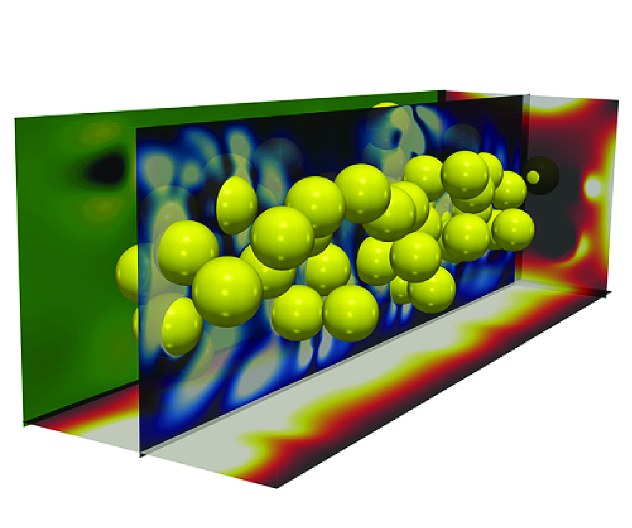
Figure 1. A 3-D view of the computational domain with solid volume fraction
 $\phi = 10\, \%$
. Trains of particles are formed at the duct corners due to the particle migration towards the walls.Here,
$\phi = 10\, \%$
. Trains of particles are formed at the duct corners due to the particle migration towards the walls.Here,
 $N_1$
,
$N_1$
,
 $U$
and
$U$
and
 $\tau _{xz}$
represent the first normal stress difference, streamwise velocity, and EVP shear stress in their corresponding planes.
$\tau _{xz}$
represent the first normal stress difference, streamwise velocity, and EVP shear stress in their corresponding planes.
2.1. Governing equations
The suspending fluid motion is governed by the incompressibility constraint and conservation of momentum as follows:
 \begin{align} \boldsymbol{\nabla} \boldsymbol{\cdot} \boldsymbol {u}& = 0, \end{align}
 \begin{align} \frac {\partial \boldsymbol {u}}{\partial t} + (\boldsymbol {u}\boldsymbol{\cdot} \boldsymbol{\nabla} ) \boldsymbol {u} &= -\boldsymbol {\nabla }{p} + \frac {\beta _s}{Re}\,\nabla ^2 \boldsymbol {u} + \boldsymbol{\nabla} \boldsymbol{\cdot} \boldsymbol {\tau }^p + \boldsymbol {f}. \end{align}
Here,
 $\boldsymbol {u}$
is the fluid velocity,
$\boldsymbol {u}$
is the fluid velocity,
 $p$
is the pressure field,
$p$
is the pressure field,
 $\boldsymbol {\tau }^p$
is the polymeric stress tensor, and
$\boldsymbol {\tau }^p$
is the polymeric stress tensor, and
 $Re$
is the Reynolds number. The extra term
$Re$
is the Reynolds number. The extra term
 $\boldsymbol {f}$
on the right-hand side of (2.2) is the immersed boundary force field representing the particle–fluid interaction; details of the immersed boundary method are given in § 2.2. Note that the stress tensor
$\boldsymbol {f}$
on the right-hand side of (2.2) is the immersed boundary force field representing the particle–fluid interaction; details of the immersed boundary method are given in § 2.2. Note that the stress tensor
 $\boldsymbol {\tau }$
is composed of the contributions from the solvent (Newtonian fluid) and polymer stresses as
$\boldsymbol {\tau }$
is composed of the contributions from the solvent (Newtonian fluid) and polymer stresses as
 $\boldsymbol {\tau } = \boldsymbol {\tau }^s + \boldsymbol {\tau }^p$
. The solvent stress tensor is defined as
$\boldsymbol {\tau } = \boldsymbol {\tau }^s + \boldsymbol {\tau }^p$
. The solvent stress tensor is defined as
 $\boldsymbol {\tau }^s = \beta _s (\boldsymbol {\nabla }{\boldsymbol {u}} + \boldsymbol {\nabla }{\boldsymbol {u}}^{\mathrm {T}})$
, where
$\boldsymbol {\tau }^s = \beta _s (\boldsymbol {\nabla }{\boldsymbol {u}} + \boldsymbol {\nabla }{\boldsymbol {u}}^{\mathrm {T}})$
, where
 $\beta _s = \mu _s/\mu$
is the ratio of the solvent viscosity to the total viscosity. In all our simulations, the viscosity ratio is fixed at
$\beta _s = \mu _s/\mu$
is the ratio of the solvent viscosity to the total viscosity. In all our simulations, the viscosity ratio is fixed at
 $\beta _s = 0.1$
. In addition to the equations mentioned earlier, a constitutive equation is needed to model the evolution of the non-Newtonian contribution (
$\beta _s = 0.1$
. In addition to the equations mentioned earlier, a constitutive equation is needed to model the evolution of the non-Newtonian contribution (
 $\boldsymbol {\tau }^p$
) of the EVP material. Since the Saramito model predicts a constant polymeric viscosity, we incorporate the Giesekus modification of the Saramito equation to account for the second normal stress difference and the shear-thinning behaviour of the EVP carrier fluid:
$\boldsymbol {\tau }^p$
) of the EVP material. Since the Saramito model predicts a constant polymeric viscosity, we incorporate the Giesekus modification of the Saramito equation to account for the second normal stress difference and the shear-thinning behaviour of the EVP carrier fluid:
 \begin{align} Wi\; \overset {\triangledown }{\boldsymbol {\tau }^p} + F\left (\boldsymbol {\tau }^p + \frac {Wi \,\,\alpha }{1-\beta _s}(\boldsymbol {\tau }^p\boldsymbol{\cdot} \boldsymbol {\tau }^p)\right ) = \frac {2(1 - \beta _s)}{Re}\, \boldsymbol {D}, \end{align}
where
 $\boldsymbol {D}\equiv 1/2 (\boldsymbol {\nabla }{\boldsymbol {u}}+\boldsymbol {\nabla }{\boldsymbol {u}}^{\mathrm {T}})$
,
$\boldsymbol {D}\equiv 1/2 (\boldsymbol {\nabla }{\boldsymbol {u}}+\boldsymbol {\nabla }{\boldsymbol {u}}^{\mathrm {T}})$
,
 $F = \max (0, ({|\boldsymbol {\tau }^p_d| - Bi/Re})/ ({|\boldsymbol {\tau }^p_d|}))$
represents the existence of yield stress in the model,
$F = \max (0, ({|\boldsymbol {\tau }^p_d| - Bi/Re})/ ({|\boldsymbol {\tau }^p_d|}))$
represents the existence of yield stress in the model,
 $Bi$
is the Bingham number,
$Bi$
is the Bingham number,
 $\alpha$
is the shear-thinning factor with
$\alpha$
is the shear-thinning factor with
 $0 \lt \alpha \lt 1$
corresponding to shear-thinning behaviour, and
$0 \lt \alpha \lt 1$
corresponding to shear-thinning behaviour, and
 $|\boldsymbol {\tau }^p_d|\equiv \sqrt {\boldsymbol {\tau }^p_d : \boldsymbol {\tau }^p_d /2}$
, with
$|\boldsymbol {\tau }^p_d|\equiv \sqrt {\boldsymbol {\tau }^p_d : \boldsymbol {\tau }^p_d /2}$
, with
 $\boldsymbol {\tau }^p_d = \boldsymbol {\tau }^p - (\mathrm {tr}\,\boldsymbol {\tau }^p/\mathrm {tr}\,{\boldsymbol {I}})\, \boldsymbol {I}$
the deviatoric part of
$\boldsymbol {\tau }^p_d = \boldsymbol {\tau }^p - (\mathrm {tr}\,\boldsymbol {\tau }^p/\mathrm {tr}\,{\boldsymbol {I}})\, \boldsymbol {I}$
the deviatoric part of
 $\boldsymbol {\tau }^p$
, and
$\boldsymbol {\tau }^p$
, and
 $\boldsymbol {I}$
the identity tensor. The upper-convected derivative of the polymer stress tensor,
$\boldsymbol {I}$
the identity tensor. The upper-convected derivative of the polymer stress tensor,
 $\overset {\triangledown }{\boldsymbol {\tau }^p}$
, is defined as
$\overset {\triangledown }{\boldsymbol {\tau }^p}$
, is defined as
 \begin{align} \overset {\triangledown }{\boldsymbol {\tau }^p} \equiv \frac {\partial \boldsymbol {\tau }^p}{\partial t} + \boldsymbol{u}\boldsymbol{\cdot} \boldsymbol {\nabla }\boldsymbol {\tau }^p - \boldsymbol {\nabla }\boldsymbol {u}^{\mathrm {T}}\boldsymbol{\cdot} \boldsymbol {\tau }^p - \boldsymbol {\tau }^p\boldsymbol{\cdot} \boldsymbol {\nabla }\boldsymbol {u}. \end{align}
The particle translational and rotational velocities are obtained by solving Newton–Euler equations for each particle as follows:
 \begin{align} \rho _p \, V_p \, \frac {\mathrm {d} \boldsymbol {u}_p}{\mathrm {d} t} &= \oint _{\partial V} \boldsymbol \sigma \boldsymbol{\cdot} \boldsymbol n \, \mathrm {d}A + \boldsymbol F_c, \end{align}
 \begin{align} I_p \, \frac {\mathrm {d} \boldsymbol \omega _p}{\mathrm {d} t}& = \oint _{\partial V} \boldsymbol r\times (\boldsymbol \sigma \boldsymbol{\cdot} \boldsymbol n) \, \mathrm {d}A + \boldsymbol T_c, \end{align}
where
 $\boldsymbol {u}_p$
and
$\boldsymbol {u}_p$
and
 $\boldsymbol \omega _p$
are the linear velocity of the centre of mass and angular velocity of the particle, and the density, volume and moment of inertia of the particle are denoted by
$\boldsymbol \omega _p$
are the linear velocity of the centre of mass and angular velocity of the particle, and the density, volume and moment of inertia of the particle are denoted by
 $\rho _p$
,
$\rho _p$
,
 $V_p$
and
$V_p$
and
 $I_p$
, respectively. Moreover,
$I_p$
, respectively. Moreover,
 $\boldsymbol {r}$
denotes the distance from the centre of the particle, and
$\boldsymbol {r}$
denotes the distance from the centre of the particle, and
 $\partial V$
represents the particle volume. Finally, the Cauchy stress tensor
$\partial V$
represents the particle volume. Finally, the Cauchy stress tensor
 $\boldsymbol {\sigma } = -p\boldsymbol {I} + \boldsymbol {\tau }^p + \beta _s (\boldsymbol {\nabla }{\boldsymbol {u}} + \boldsymbol {\nabla }{\boldsymbol {u}}^{\mathrm {T}})$
and
$\boldsymbol {\sigma } = -p\boldsymbol {I} + \boldsymbol {\tau }^p + \beta _s (\boldsymbol {\nabla }{\boldsymbol {u}} + \boldsymbol {\nabla }{\boldsymbol {u}}^{\mathrm {T}})$
and
 $\boldsymbol {F}_c$
and
$\boldsymbol {F}_c$
and
 $\boldsymbol {T}_c$
represent the total force and torque generated by particle–particle/wall collisions. To model these short-range particle–particle/wall interactions, a soft-sphere collision model with lubrication correction is employed as described by Costa et al. (Reference Costa, Boersma, Westerweel and Breugem2015).
$\boldsymbol {T}_c$
represent the total force and torque generated by particle–particle/wall collisions. To model these short-range particle–particle/wall interactions, a soft-sphere collision model with lubrication correction is employed as described by Costa et al. (Reference Costa, Boersma, Westerweel and Breugem2015).
2.2. Numerical method
The numerical code is based on a direct forcing immersed boundary method (IBM) to simulate the dispersed phase as moving Lagrangian grids, while the carrier fluid is discretised on a fixed Eulerian frame, in which the fluid momentum and the constitutive equations are discretised using finite differences. The fluid momentum solver employs a projection method (pressure correction) to decouple the computations of the velocity and pressure fields, and implements a highly efficient and scalable fast Fourier transform based method to solve the pressure Poisson equation. In addition, spatial derivatives in flow equations are approximated by a central finite difference scheme, with the exception of the advection term in the constitutive equation, which is discretised using the fifth-order WENO method (Shu Reference Shu2009). A third-order Runge–Kutta scheme is used to integrate the governing equations in time.
The fluid–solid interaction is simulated by a direct forcing IBM first proposed by Uhlmann (Reference Uhlmann2005) and further improved by Breugem (Reference Breugem2012) to simulate particle motions with second-order spatial accuracy. In the IBM, the fluid is represented by a uniform (
 $\Delta x = \Delta y = \Delta z$
) staggered Cartesian grid, and the particle interface is represented by a collection of moving Lagrangian points that are uniformly distributed on the surface of the particle. The fluid momentum equations are solved on the entire grid, and the effect of the presence of the particles is modelled by adding an extra force
$\Delta x = \Delta y = \Delta z$
) staggered Cartesian grid, and the particle interface is represented by a collection of moving Lagrangian points that are uniformly distributed on the surface of the particle. The fluid momentum equations are solved on the entire grid, and the effect of the presence of the particles is modelled by adding an extra force
 $\boldsymbol {f}$
on the right-hand side of (2.2), active in the immediate vicinity of the solid boundary to enforce the no-slip/no-penetration condition on the surface of the particles (Mittal & Iaccarino Reference Mittal and Iaccarino2005). The obtained immersed boundary force is applied to both dispersed and carrier phases to update the velocities in time. The reader can find detailed explanations of the numerical approach used in the present work in our previous studies (Ardekani et al. Reference Ardekani, Costa, Breugem and Brandt2016; Izbassarov et al. Reference Izbassarov, Rosti, Ardekani, Sarabian, Hormozi, Brandt and Tammisola2018; Niazi Ardekani Reference Ardekani2019). Note finally that we conduct box size and resolution studies to confirm that our results are not affected by any numerical artefacts (see Appendix A). Due to the high resolution employed and the relatively low lateral velocity of the particles, each simulation may require up to four weeks, utilising 160 computational cores, depending on the focusing length necessary to achieve the final steady state. In cases where we compare with experimental data (see § 2.3), we used 768 cores for up to eight weeks to capture the statistically steady-state particle distribution.
$\boldsymbol {f}$
on the right-hand side of (2.2), active in the immediate vicinity of the solid boundary to enforce the no-slip/no-penetration condition on the surface of the particles (Mittal & Iaccarino Reference Mittal and Iaccarino2005). The obtained immersed boundary force is applied to both dispersed and carrier phases to update the velocities in time. The reader can find detailed explanations of the numerical approach used in the present work in our previous studies (Ardekani et al. Reference Ardekani, Costa, Breugem and Brandt2016; Izbassarov et al. Reference Izbassarov, Rosti, Ardekani, Sarabian, Hormozi, Brandt and Tammisola2018; Niazi Ardekani Reference Ardekani2019). Note finally that we conduct box size and resolution studies to confirm that our results are not affected by any numerical artefacts (see Appendix A). Due to the high resolution employed and the relatively low lateral velocity of the particles, each simulation may require up to four weeks, utilising 160 computational cores, depending on the focusing length necessary to achieve the final steady state. In cases where we compare with experimental data (see § 2.3), we used 768 cores for up to eight weeks to capture the statistically steady-state particle distribution.
2.3. Comparison with experiments
In this subsection, we validate our numerical simulations of particle suspensions in EVP duct flows by comparing them with the experiments conductedpreviously by Zade et al. (Reference Zade, Shamu, Lundell and Brandt2020). These authors examined the collective behaviour of finite-size spherical particles in a square duct flow of a Carbopol solution (with a concentration of 0.25 % w/w). The experimental paper provides the steady shear flow curve that reveals the key rheological properties of the Carbopol fluid, including its yield stress, plastic viscosity and shear-thinning factor. Furthermore, by determining the value of the storage modulus (
 $G^{\prime }$
) at the lowest strain value from the strain amplitude sweep oscillatory test, an approximation of the material’s shear modulus (
$G^{\prime }$
) at the lowest strain value from the strain amplitude sweep oscillatory test, an approximation of the material’s shear modulus (
 $G$
) was obtained. With the known values of plastic viscosity (
$G$
) was obtained. With the known values of plastic viscosity (
 $\mu _p$
) and shear modulus (
$\mu _p$
) and shear modulus (
 $G$
), the relaxation time (
$G$
), the relaxation time (
 $\lambda$
) of the material could be calculated using the relationship
$\lambda$
) of the material could be calculated using the relationship
 $\lambda = \mu _p/G$
. The corresponding non-dimensional numbers for two distinct particle suspension cases are calculated using the non-dimensional parameters adopted in the current paper, and are presented in table 1.
$\lambda = \mu _p/G$
. The corresponding non-dimensional numbers for two distinct particle suspension cases are calculated using the non-dimensional parameters adopted in the current paper, and are presented in table 1.
Table 1. The non-dimensional numbers used for the numerical simulations from the experimental data of Zade et al. (Reference Zade, Shamu, Lundell and Brandt2020).

In figures 2(a,b), we compare the experimental velocity profiles of the EVP suspension with our numerical predictions, utilising the Saramito (Reference Saramito2009) model (depicted in blue lines). In particular, we report the mean streamwise fluid velocity profiles
 $U (y)$
, normalised by the bulk velocity (
$U (y)$
, normalised by the bulk velocity (
 $U_b$
) at various spanwise locations (
$U_b$
) at various spanwise locations (
 $z/ H$
), and at two different sets of parameters (see figure caption). Our simulations demonstrate remarkable agreement with the experimental mean flow profiles of the EVP duct flow in the presence of particles. Additionally, for the first parameter set, we compare the particle distribution from our simulations with the experimental results. We present a 3-D snapshot of the flow field with particle distribution in figure 2(c), alongside the statistically steady-state distribution of particles within the EVP flow shown in figure 2(d). The statistical particle distribution
$z/ H$
), and at two different sets of parameters (see figure caption). Our simulations demonstrate remarkable agreement with the experimental mean flow profiles of the EVP duct flow in the presence of particles. Additionally, for the first parameter set, we compare the particle distribution from our simulations with the experimental results. We present a 3-D snapshot of the flow field with particle distribution in figure 2(c), alongside the statistically steady-state distribution of particles within the EVP flow shown in figure 2(d). The statistical particle distribution
 $\Phi (y,z)$
represents the time and spatial averaged concentration of the solid phase in the duct cross-section (see Appendix D for the definition of averaged solid concentration
$\Phi (y,z)$
represents the time and spatial averaged concentration of the solid phase in the duct cross-section (see Appendix D for the definition of averaged solid concentration
 $\Phi$
). This visualisation demonstrates that the particles accumulate in a ring-like formation between the centre of the duct and the walls. This prediction aligns with the experimental findings. However, our simulations reveal an additional feature: a small fraction of the particles accumulates at the corners of the duct. This behaviour was not observed in the experiments, likely due to the limited duct length (5 m in the laboratory experiments), which may not have been sufficient for the particles to reach their stable positions. In contrast, our simulations, which were conducted over times significantly longer than those needed to travel 5 m, capture the migration of some particles towards the corners. In § 3, we comprehensively discuss the effects of the particle volume fraction, yield stress, elasticity, inertia (Reynolds number) and shear-thinning on the particle distribution.
$\Phi$
). This visualisation demonstrates that the particles accumulate in a ring-like formation between the centre of the duct and the walls. This prediction aligns with the experimental findings. However, our simulations reveal an additional feature: a small fraction of the particles accumulates at the corners of the duct. This behaviour was not observed in the experiments, likely due to the limited duct length (5 m in the laboratory experiments), which may not have been sufficient for the particles to reach their stable positions. In contrast, our simulations, which were conducted over times significantly longer than those needed to travel 5 m, capture the migration of some particles towards the corners. In § 3, we comprehensively discuss the effects of the particle volume fraction, yield stress, elasticity, inertia (Reynolds number) and shear-thinning on the particle distribution.

Figure 2. Validation of numerical simulations against experiments by Zade et al. (Reference Zade, Shamu, Lundell and Brandt2020). Simulated mean streamwise fluid velocity profiles (
 $U / U_{bulk}$
), denoted by blue lines, compared against the experimental data represented by red symbols at (a)
$U / U_{bulk}$
), denoted by blue lines, compared against the experimental data represented by red symbols at (a)
 $Re = 36.7$
,
$Re = 36.7$
,
 $Bi = 0.14$
,
$Bi = 0.14$
,
 $Wi = 0.26$
,
$Wi = 0.26$
,
 $\beta _s = 0.11$
,
$\beta _s = 0.11$
,
 $\kappa = 1/12$
,
$\kappa = 1/12$
,
 $\phi = 5\, \%$
, and (b)
$\phi = 5\, \%$
, and (b)
 $Re = 13$
,
$Re = 13$
,
 $Bi = 0.2$
,
$Bi = 0.2$
,
 $Wi = 0.182$
,
$Wi = 0.182$
,
 $\beta _s = 0.16$
,
$\beta _s = 0.16$
,
 $\kappa = 1/12$
,
$\kappa = 1/12$
,
 $\phi = 5\, \%$
. (c) A 3-D snapshot of particle suspension showing particle distribution and contours of the first normal stress difference (
$\phi = 5\, \%$
. (c) A 3-D snapshot of particle suspension showing particle distribution and contours of the first normal stress difference (
 $N_1$
) and streamwise velocity (
$N_1$
) and streamwise velocity (
 $U$
). (d) Statistical distribution of the particles across the duct section from our simulations.
$U$
). (d) Statistical distribution of the particles across the duct section from our simulations.
3. Results
In this section, numerical simulations of particle migration in EVP duct flow are discussed. The study explores a range of parameters, including particle volume fractions (
 $\phi$
) from 0 % to 20 %, Bingham numbers (
$\phi$
) from 0 % to 20 %, Bingham numbers (
 $Bi$
) from 0 to 4, and Weissenberg numbers (
$Bi$
) from 0 to 4, and Weissenberg numbers (
 $Wi$
) from 0 to 1, while accounting for shear-thinning viscosity. In § 3.1, we first examine the steady-state flow field for three representative cases. Subsequently, we analyse the dynamics governing particle migration by investigating stress fields and secondary flows. Finally, in §§ 3.2–3.4, we explore the effect of the governing parameters on the distribution of particles. A summary of the simulated cases is provided in table 2.
$Wi$
) from 0 to 1, while accounting for shear-thinning viscosity. In § 3.1, we first examine the steady-state flow field for three representative cases. Subsequently, we analyse the dynamics governing particle migration by investigating stress fields and secondary flows. Finally, in §§ 3.2–3.4, we explore the effect of the governing parameters on the distribution of particles. A summary of the simulated cases is provided in table 2.
Table 2. Overview of the range of non-dimensional numbers used in our simulations. Here,
 $L_x$
,
$L_x$
,
 $L_y$
and
$L_y$
and
 $L_z$
are given in units of particle diameter.
$L_z$
are given in units of particle diameter.

3.1. Steady-state particle distribution

Figure 3. Instantaneous snapshots of flow field (left-hand column) and mean particle concentration
 $\Phi (x,z)$
(right-hand column) across the duct section in (a) Newtonian, (b) Saramito EVP with
$\Phi (x,z)$
(right-hand column) across the duct section in (a) Newtonian, (b) Saramito EVP with
 $El=0.05$
,
$El=0.05$
,
 $Bi = 0.2$
, and (c) Saramito–Giesekus with
$Bi = 0.2$
, and (c) Saramito–Giesekus with
 $El=0.05$
,
$El=0.05$
,
 $Bi = 0.2$
,
$Bi = 0.2$
,
 $\alpha = 0.2$
carrier fluids. In all cases, the volume fraction
$\alpha = 0.2$
carrier fluids. In all cases, the volume fraction
 $\phi$
is 10 %, and
$\phi$
is 10 %, and
 $Re=20$
. Contours in the 3-D snapshotsdepict: (a) streamwise velocity (
$Re=20$
. Contours in the 3-D snapshotsdepict: (a) streamwise velocity (
 $U$
) and secondary flows (
$U$
) and secondary flows (
 $\sqrt {V^2 + W^2}$
); (b,c) the first normal stress difference (
$\sqrt {V^2 + W^2}$
); (b,c) the first normal stress difference (
 $N_1$
) and
$N_1$
) and
 $U$
.
$U$
.
Figure 3 presents 3-D instantaneous snapshots of the flow field and the particle distribution in Newtonian (figure 3
a), Saramito (figure 3
b), and Saramito–Giesekus (figure 3
c) carrier fluids after the flow field and particle positions have reached their statistically steady state. In addition, to provide a better understanding of particle distribution across the duct cross-section, the mean particle concentration
 $\Phi (y,z)$
of solid spheres is illustrated for each of the suspensions. In all cases, the Reynolds number is
$\Phi (y,z)$
of solid spheres is illustrated for each of the suspensions. In all cases, the Reynolds number is
 $Re = 20$
, the solid volume fraction is
$Re = 20$
, the solid volume fraction is
 $\phi = 10\, \%$
, and the blockage ratio is
$\phi = 10\, \%$
, and the blockage ratio is
 $\kappa = 0.2$
. For EVP suspensions, the elasticity number is fixed at
$\kappa = 0.2$
. For EVP suspensions, the elasticity number is fixed at
 $El = 0.05$
, and the Bingham number is
$El = 0.05$
, and the Bingham number is
 $Bi = 0.2$
. The Saramito fluid assumes a zero shear-thinning factor (indicating a constant polymer viscosity), while the Saramito–Giesekus case uses
$Bi = 0.2$
. The Saramito fluid assumes a zero shear-thinning factor (indicating a constant polymer viscosity), while the Saramito–Giesekus case uses
 $\alpha = 0.2$
, introducing shear-thinning behaviour to the carrier fluid.
$\alpha = 0.2$
, introducing shear-thinning behaviour to the carrier fluid.
In the Newtonian case, particles eventually accumulate between the duct centre and the walls, forming a square shape with the highest concentration of particles at the corners of the square. In contrast, the Saramito (EVP) fluid induces central migration, enabling particles to penetrate the central plug region and form a large cluster. On the other hand, the Saramito–Giesekus fluid causes particles to migrate towards the duct walls, leading to distinct particle chain formations at the corners. These varied behaviours can be largely attributed to the rheological characteristics of the carrier fluids.
The distribution of the first normal stress difference, defined as
 $N_1 = \tau _{xx}^p - \tau _{yy}^p$
, is depicted across various planes in 3-D snapshots. This normal stress difference reflects the tension acting in the direction of the streamlines. Streamlines under tension curve around the particles, and the lateral forces exerted on each side of a particle create a hoop thrust that drives the particle towards the region with the lowest normal stress difference (Ho & Leal Reference Ho and Leal1976). As illustrated in the figure,
$N_1 = \tau _{xx}^p - \tau _{yy}^p$
, is depicted across various planes in 3-D snapshots. This normal stress difference reflects the tension acting in the direction of the streamlines. Streamlines under tension curve around the particles, and the lateral forces exerted on each side of a particle create a hoop thrust that drives the particle towards the region with the lowest normal stress difference (Ho & Leal Reference Ho and Leal1976). As illustrated in the figure,
 $N_1$
reaches its peak values near the duct walls, while it is considerably lower in proximity to the centre and corners of the duct. Consequently, the gradient of the first normal stress difference tends to propel particles towards the duct centre, where they experience the least elastic stress. This aggregation phenomenon is especially notable in the Saramito fluid model, where particles concentrate significantly in the central region of the duct (see figure 3
b).
$N_1$
reaches its peak values near the duct walls, while it is considerably lower in proximity to the centre and corners of the duct. Consequently, the gradient of the first normal stress difference tends to propel particles towards the duct centre, where they experience the least elastic stress. This aggregation phenomenon is especially notable in the Saramito fluid model, where particles concentrate significantly in the central region of the duct (see figure 3
b).
The shear-thinning viscosity, represented by the nonlinear term in the Saramito–Giesekus equation
 $ ({Wi\, \alpha }/{(1-\beta _s)})(\boldsymbol {\tau }^p\boldsymbol{\cdot} \boldsymbol {\tau }^p)$
, contributes to the concentration of particles at the corners of the duct. The influence of shear-thinning on particle migration is twofold. First, the reduction in viscosity with increasing shear rate within shear-thinning fluids promotes a more uniform velocity profile, characterised by a flattened centre and steeper gradients near the walls. The elevated shear gradients adjacent to the walls generate stronger inertial forces that drive the particles towards the duct walls. Additionally, the nonlinear term in the constitutive equation attenuates the first normal stress difference in EVP fluid flow, as reflected in the
$ ({Wi\, \alpha }/{(1-\beta _s)})(\boldsymbol {\tau }^p\boldsymbol{\cdot} \boldsymbol {\tau }^p)$
, contributes to the concentration of particles at the corners of the duct. The influence of shear-thinning on particle migration is twofold. First, the reduction in viscosity with increasing shear rate within shear-thinning fluids promotes a more uniform velocity profile, characterised by a flattened centre and steeper gradients near the walls. The elevated shear gradients adjacent to the walls generate stronger inertial forces that drive the particles towards the duct walls. Additionally, the nonlinear term in the constitutive equation attenuates the first normal stress difference in EVP fluid flow, as reflected in the
 $N_1$
contours from the snapshots. The Saramito fluid exhibits first normal stress difference values ranging from 0 to 2, while the Saramito–Giesekus fluid demonstrates lower
$N_1$
contours from the snapshots. The Saramito fluid exhibits first normal stress difference values ranging from 0 to 2, while the Saramito–Giesekus fluid demonstrates lower
 $N_1$
values, between 0 and 0.5. This decrease in
$N_1$
values, between 0 and 0.5. This decrease in
 $N_1$
leads to a reduction in viscoelastic forces, which consequently weakens the tendency of particles to migrate towards the central region of the flow. As a result, in highly shear-thinning fluids, such as the Saramito–Giesekus fluid (
$N_1$
leads to a reduction in viscoelastic forces, which consequently weakens the tendency of particles to migrate towards the central region of the flow. As a result, in highly shear-thinning fluids, such as the Saramito–Giesekus fluid (
 $\alpha = 0.2$
), particles are preferentially directed towards the walls and corners of the duct, rather than towards its centre.
$\alpha = 0.2$
), particles are preferentially directed towards the walls and corners of the duct, rather than towards its centre.
Figure 4 illustrates different components of the polymeric stress tensor in the duct cross-section of the Saramito–Giesekus suspension. The values are obtained by calculating the average of the polymeric stress in several cross-sections along the streamwise direction and over time. The primary component of shear polymeric stress,
 $\tau _{xy}^p$
, ranges between
$\tau _{xy}^p$
, ranges between
 $-0.08$
and
$-0.08$
and
 $0.08$
. The values of
$0.08$
. The values of
 $\tau _{xz}^p$
exhibit a similar range, but are rotated by
$\tau _{xz}^p$
exhibit a similar range, but are rotated by
 $90^\circ$
due to symmetry (
$90^\circ$
due to symmetry (
 $\tau _{xz}^p$
is not included in the plot to avoid redundancy). On the other hand, the values of
$\tau _{xz}^p$
is not included in the plot to avoid redundancy). On the other hand, the values of
 $\tau _{yz}^p$
are one order of magnitude lower, ranging from
$\tau _{yz}^p$
are one order of magnitude lower, ranging from
 $-5.5 \times 10^{-3}$
to
$-5.5 \times 10^{-3}$
to
 $5.5 \times 10^{-3}$
. The first and second normal stresses,
$5.5 \times 10^{-3}$
. The first and second normal stresses,
 $N_1 = \tau _{xx}^p - \tau _{yy}^p$
and
$N_1 = \tau _{xx}^p - \tau _{yy}^p$
and
 $N_2 = \tau _{yy}^p - \tau _{zz}^p$
, are displayed in figures 4(b,d), and represent the tension present along and perpendicular to the direction of flow (Bird et al. Reference Bird, Armstrong and Hassager1987). For the flow under consideration, the maximum of
$N_2 = \tau _{yy}^p - \tau _{zz}^p$
, are displayed in figures 4(b,d), and represent the tension present along and perpendicular to the direction of flow (Bird et al. Reference Bird, Armstrong and Hassager1987). For the flow under consideration, the maximum of
 $N_2$
is about one order of magnitude smaller than the maximum of
$N_2$
is about one order of magnitude smaller than the maximum of
 $N_1$
.
$N_1$
.

Figure 4. Polymeric stress components in the suspension with solid volume fraction
 $\phi = 10\, \%$
in the EVP carrier fluid: (a)
$\phi = 10\, \%$
in the EVP carrier fluid: (a)
 $\tau _{xy}^p$
, (b)
$\tau _{xy}^p$
, (b)
 $N_1 = \tau _{xx}^p - \tau _{yy}^p$
, (c)
$N_1 = \tau _{xx}^p - \tau _{yy}^p$
, (c)
 $\tau _{yz}^p$
, and (d)
$\tau _{yz}^p$
, and (d)
 $N_2 = \tau _{yy}^p - \tau _{zz}^p$
.
$N_2 = \tau _{yy}^p - \tau _{zz}^p$
.

Figure 5. Secondary flows in (a) Newtonian suspension and (b) EVP suspension, with
 $Bi = 0.2$
,
$Bi = 0.2$
,
 $El = 0.05$
and
$El = 0.05$
and
 $\alpha = 0.2$
. For both cases,
$\alpha = 0.2$
. For both cases,
 $\phi = 10\, \%$
and
$\phi = 10\, \%$
and
 $Re = 20$
.
$Re = 20$
.
Despite its low magnitude, the second normal stress difference can cause secondary flows within the cross-section of viscoelastic duct flows, which can significantly affect the migration of particles. Figure 5 depicts the secondary flows consisting of eight vortices develop in both Newtonian and EVP suspensions at particle volume fraction
 $\phi = 10\, \%$
. The maximum magnitude of secondary flows in the EVP suspension is
$\phi = 10\, \%$
. The maximum magnitude of secondary flows in the EVP suspension is
 $8.4 \times 10^{-3}$
, which is 3.2 times greater than in the Newtonian suspension. This suggests that the second normal stress differences present in the EVP fluid enhance the secondary flows that are solely induced by the particles in Newtonian suspensions. Since the magnitude of secondary flows reaches
$8.4 \times 10^{-3}$
, which is 3.2 times greater than in the Newtonian suspension. This suggests that the second normal stress differences present in the EVP fluid enhance the secondary flows that are solely induced by the particles in Newtonian suspensions. Since the magnitude of secondary flows reaches
 $O(10^{-2})$
of the mean flow velocity, which is comparable to cross-streamline migration velocity
$O(10^{-2})$
of the mean flow velocity, which is comparable to cross-streamline migration velocity
 $O(10^{-3})$
, these secondary flows are strong enough to push the particles away from the centre towards the walls and corners.
$O(10^{-3})$
, these secondary flows are strong enough to push the particles away from the centre towards the walls and corners.
To summarise, in the Saramito–Giesekus carrier fluid, with a high enough elasticity, the combination of elastic forces, shear-thinning viscosity, and the presence of secondary flows, causes particles to concentrate at the duct corners, leaving the core of the duct almost particle-free.
In the following subsections, we provide further insight into the physical mechanisms driving particle migration in EVP fluids by investigating the effects of solid volume fraction, elasticity and yield stress on the final distribution of particles.
3.2. Effect of solid volume fraction

Figure 6. The steady distributions of particles at
 $\phi =3.5\,\%$
,
$\phi =3.5\,\%$
,
 $10\,\%$
and
$10\,\%$
and
 $ 20\, \%$
, respectively, across the duct sections of (a,b,c) Newtonian and (d,e,f) Saramito–Giesekus carrier fluids with
$ 20\, \%$
, respectively, across the duct sections of (a,b,c) Newtonian and (d,e,f) Saramito–Giesekus carrier fluids with
 $Re=20$
,
$Re=20$
,
 $Bi = 0.2$
,
$Bi = 0.2$
,
 $El = 0.05$
and
$El = 0.05$
and
 $\alpha = 0.2$
.
$\alpha = 0.2$
.

Figure 7. (a) The streamwise mean velocity profile for the EVP suspensions at
 $\phi = 0\,\%$
,
$\phi = 0\,\%$
,
 $3.5\,\%$
,
$3.5\,\%$
,
 $10\,\%$
and
$10\,\%$
and
 $ 20\, \%$
. (b) Comparison of particle and fluid velocities at
$ 20\, \%$
. (b) Comparison of particle and fluid velocities at
 $z/H = 0.8$
(near the wall) and
$z/H = 0.8$
(near the wall) and
 $z/H = 0$
(duct centre) for EVP suspensions with
$z/H = 0$
(duct centre) for EVP suspensions with
 $\phi = 20\, \%$
(left) and
$\phi = 20\, \%$
(left) and
 $\phi = 10\, \%$
(right).
$\phi = 10\, \%$
(right).
Figure 6 shows the mean concentration of particles for
 $\phi=3.5\,\%$
,
$\phi=3.5\,\%$
,
 $10\,\%$
and
$10\,\%$
and
 $ 20\, \%$
in Newtonian and Saramito–Giesekus carrier fluids with
$ 20\, \%$
in Newtonian and Saramito–Giesekus carrier fluids with
 $Re = 20$
,
$Re = 20$
,
 $\kappa =0.2$
,
$\kappa =0.2$
,
 $El = 0.05$
and
$El = 0.05$
and
 $Bi = 0.2$
. In the Newtonian dilute suspension
$Bi = 0.2$
. In the Newtonian dilute suspension
 $\phi=3.5\,\%$
, inertial effects are dominant and the particles accumulate near the centre of duct walls at a distance approximately 0.3 from the duct centre (see figure 6
a). A similar pattern occurs in the suspension with
$\phi=3.5\,\%$
, inertial effects are dominant and the particles accumulate near the centre of duct walls at a distance approximately 0.3 from the duct centre (see figure 6
a). A similar pattern occurs in the suspension with
 $\phi =10\,\%$
, where particles focus in a square between the centre and the walls (figure 6
b). Most of the particles are preferentially accumulated at the corners of this smaller square, and less at the wall middle planes. It is worth mentioning that the duct core is depleted of particles in both dilute and semi-dilute Newtonian suspensions. This is due to the inertial lift force that makes the duct core an unstable location by pushing the particles towards the walls. At the highest volume fraction
$\phi =10\,\%$
, where particles focus in a square between the centre and the walls (figure 6
b). Most of the particles are preferentially accumulated at the corners of this smaller square, and less at the wall middle planes. It is worth mentioning that the duct core is depleted of particles in both dilute and semi-dilute Newtonian suspensions. This is due to the inertial lift force that makes the duct core an unstable location by pushing the particles towards the walls. At the highest volume fraction
 $\phi =20\,\%$
, inertial focusing completely breaks down, and particles accumulate at the duct core (figure 6
c). The increase in solid volume fraction enhances the particle–wall and particle–particle collisions, and increases shear-induced migration that makes particles in concentrated suspensions migrate to low-shear regions (Leighton & Acrivos Reference Leighton and Acrivos1987), which results in particles leaving the walls and preferentially moving in the centre of the duct. At Reynolds number 20, inertial effects are not strong enough to push the particles away from the centre and counterbalance collision-dominated shear-induced migration (Kazerooni et al. Reference Kazerooni, Fornari, Hussong and Brandt2017). In other words, the particle–particle collisions overcome the inertial effects and make the duct core a stable position for the particles.
$\phi =20\,\%$
, inertial focusing completely breaks down, and particles accumulate at the duct core (figure 6
c). The increase in solid volume fraction enhances the particle–wall and particle–particle collisions, and increases shear-induced migration that makes particles in concentrated suspensions migrate to low-shear regions (Leighton & Acrivos Reference Leighton and Acrivos1987), which results in particles leaving the walls and preferentially moving in the centre of the duct. At Reynolds number 20, inertial effects are not strong enough to push the particles away from the centre and counterbalance collision-dominated shear-induced migration (Kazerooni et al. Reference Kazerooni, Fornari, Hussong and Brandt2017). In other words, the particle–particle collisions overcome the inertial effects and make the duct core a stable position for the particles.
In the Saramito–Giesekus suspension, the distribution of particles displays a similar pattern for
 $\phi =3.5\,\%$
and
$\phi =3.5\,\%$
and
 $\phi =10\,\%$
, where the particles are mainly focused at the duct corners and walls, while the duct core is completely free of particles. Even when the solid volume fraction is at its highest,
$\phi =10\,\%$
, where the particles are mainly focused at the duct corners and walls, while the duct core is completely free of particles. Even when the solid volume fraction is at its highest,
 $\phi =20\, \%$
, the majority of particles still tend to aggregate near the corners and walls of the duct. Nonetheless, excluded volume effects cannot be neglected at the solid volume fraction
$\phi =20\, \%$
, the majority of particles still tend to aggregate near the corners and walls of the duct. Nonetheless, excluded volume effects cannot be neglected at the solid volume fraction
 $\phi =20\, \%$
, and we observe a more uniform distribution across the cross-section, including some particles reaching the duct centre.
$\phi =20\, \%$
, and we observe a more uniform distribution across the cross-section, including some particles reaching the duct centre.
The effect of solid volume fraction on the streamwise velocity, normalised by the bulk velocity, is shown in figure 7(a) for the three particle suspensions under investigation and the single-phase EVP flow. In the single-phase case, a plug region appears in the middle of the duct due to the lack of sufficient shear stress to yield the EVP material. As a result, the material in the duct core has a solid-like behaviour, and the velocity profile of the single-phase EVP flow is flat at the centre. When compared to the single-phase Newtonian flow, the presence of the plug region reduces the maximum velocity at the core (from
 $U_{max}= 2.2$
in Newtonian single-phaseflow to
$U_{max}= 2.2$
in Newtonian single-phaseflow to
 $U_{max}= 1.6$
in EVP single-phase flow). Interestingly, in the particulate cases, no flat profile appears at this value of the Bingham number when the particle-induced stresses can break and yield the plug regions, causing the velocity field to more closely resemble that of a single-phase Newtonian flow. As a result, the maximum velocity of the suspension flow exceeds the maximum velocity in the single-phase flow (from
$U_{max}= 1.6$
in EVP single-phase flow). Interestingly, in the particulate cases, no flat profile appears at this value of the Bingham number when the particle-induced stresses can break and yield the plug regions, causing the velocity field to more closely resemble that of a single-phase Newtonian flow. As a result, the maximum velocity of the suspension flow exceeds the maximum velocity in the single-phase flow (from
 $U_{max}= 1.6$
in EVP single-phaseflow to
$U_{max}= 1.6$
in EVP single-phaseflow to
 $U_{max}= 1.7{-}1.9$
in the particulate flows). Closer to the wall, the maximum velocity of the single phase is greater than in particulate cases due to the additional resistance imposed by the particle wall layer. It is noteworthy that the central velocity of the EVP suspension with
$U_{max}= 1.7{-}1.9$
in the particulate flows). Closer to the wall, the maximum velocity of the single phase is greater than in particulate cases due to the additional resistance imposed by the particle wall layer. It is noteworthy that the central velocity of the EVP suspension with
 $\phi=20\,\%$
is lower than that of the suspension with
$\phi=20\,\%$
is lower than that of the suspension with
 $\phi=10\,\%$
. This can be attributed to the homogeneous distribution of particles across the cross-section of the duct at the highest volume fraction, which reduces the maximum velocity of the flow.
$\phi=10\,\%$
. This can be attributed to the homogeneous distribution of particles across the cross-section of the duct at the highest volume fraction, which reduces the maximum velocity of the flow.
To further examine this behaviour, we present the streamwise velocities of both particles (
 $U_p$
) and fluid (
$U_p$
) and fluid (
 $U_f$
) at
$U_f$
) at
 $z/H = 0.8$
(near the wall) and
$z/H = 0.8$
(near the wall) and
 $z/H = 0$
(duct midplane) along the
$z/H = 0$
(duct midplane) along the
 $y$
-axis for EVP suspensions with
$y$
-axis for EVP suspensions with
 $\phi = 20\, \%$
(left) and
$\phi = 20\, \%$
(left) and
 $\phi = 10\, \%$
(right) in figure 7(b). In general, particle velocities closely align with the streamwise fluid velocities, except for the
$\phi = 10\, \%$
(right) in figure 7(b). In general, particle velocities closely align with the streamwise fluid velocities, except for the
 $\phi = 10\, \%$
suspension, where particles are completely absent from the duct core. Our findings reveal a significant lag between particle and fluid velocities, particularly in regions near the walls and corners (particle trains), with the solid phase moving more slowly than the surrounding fluid.
$\phi = 10\, \%$
suspension, where particles are completely absent from the duct core. Our findings reveal a significant lag between particle and fluid velocities, particularly in regions near the walls and corners (particle trains), with the solid phase moving more slowly than the surrounding fluid.
3.3. Effect of elasticity
We now consider the role of fluid elasticity on particle migration in yield-stress fluids. Figure 8 illustrates the mean concentration of particles in an EVP suspension with three different elasticity numbers, namely
 $El = 0.005, 0.025, 0.05$
. In the case with the lowest elasticity number, figure 8(a), the particle distribution is similar to the distribution of particles in a Newtonian fluid, where inertial effects are dominant, and particles find their equilibrium positions in a square located between the duct centre and the walls. As the elasticity number increases (see figures 8
b,c), the elastic forces overcome the inertial effects and the particles are pushed towards the duct corners. At the intermediate value considered here,
$El = 0.005, 0.025, 0.05$
. In the case with the lowest elasticity number, figure 8(a), the particle distribution is similar to the distribution of particles in a Newtonian fluid, where inertial effects are dominant, and particles find their equilibrium positions in a square located between the duct centre and the walls. As the elasticity number increases (see figures 8
b,c), the elastic forces overcome the inertial effects and the particles are pushed towards the duct corners. At the intermediate value considered here,
 $El=0.025$
, particles are observed everywhere along the walls, whereas when further increasing elasticity to
$El=0.025$
, particles are observed everywhere along the walls, whereas when further increasing elasticity to
 $El=0.05$
, the particles appear to be heavily focused on the corners. It is worth noting that while most of the particles are collected in the corners, some are also attached to the duct walls. While remaining in contact with the walls, these particles tend to find a place in the duct corners by making a slow rolling motion perpendicular to the flow direction with a velocity
$El=0.05$
, the particles appear to be heavily focused on the corners. It is worth noting that while most of the particles are collected in the corners, some are also attached to the duct walls. While remaining in contact with the walls, these particles tend to find a place in the duct corners by making a slow rolling motion perpendicular to the flow direction with a velocity
 $\sim O(10^{-3})$
of the particle streamwise velocity.
$\sim O(10^{-3})$
of the particle streamwise velocity.
To further interpret these observations, we consider the first normal stress difference
 $N_1$
and its average cross-stream variation when varying
$N_1$
and its average cross-stream variation when varying
 $El$
; see contour plots in figure 8. The core and corners of the duct consistently exhibit the lowest values of
$El$
; see contour plots in figure 8. The core and corners of the duct consistently exhibit the lowest values of
 $N_1$
, while the walls of the duct consistently display the highest values. Increasing the elasticity number leads to changes in the magnitude and gradients of
$N_1$
, while the walls of the duct consistently display the highest values. Increasing the elasticity number leads to changes in the magnitude and gradients of
 $N_1$
. Specifically, the average of
$N_1$
. Specifically, the average of
 $N_1$
increases from 0.067 at
$N_1$
increases from 0.067 at
 $El=0.005$
to 0.16 at
$El=0.005$
to 0.16 at
 $El=0.025$
, and the gradient of
$El=0.025$
, and the gradient of
 $N_1$
becomes steeper, suggesting a stronger influence of elastic forces on the suspended particles. The gradient is particularly pronounced around the corners and in the region between the centre and corners (see figure 8
c), which explains why particles are almost trapped in the areas with lower elastic force, i.e. the corners of the duct (see also the discussion in § 3.1 on the steady distribution of particles).
$N_1$
becomes steeper, suggesting a stronger influence of elastic forces on the suspended particles. The gradient is particularly pronounced around the corners and in the region between the centre and corners (see figure 8
c), which explains why particles are almost trapped in the areas with lower elastic force, i.e. the corners of the duct (see also the discussion in § 3.1 on the steady distribution of particles).

Figure 8. The steady distribution of particles (
 $\Phi$
), along with the first normal stress difference (
$\Phi$
), along with the first normal stress difference (
 $N_1$
) across the duct section in Saramito–Giesekus EVP carrier fluids at three different elasticity numbers: (a,d)
$N_1$
) across the duct section in Saramito–Giesekus EVP carrier fluids at three different elasticity numbers: (a,d)
 $El=0.005$
, (b,e)
$El=0.005$
, (b,e)
 $El=0.025$
, and (c,f)
$El=0.025$
, and (c,f)
 $El=0.05$
. For all cases,
$El=0.05$
. For all cases,
 $Re=20$
,
$Re=20$
,
 $Bi=0.2$
and
$Bi=0.2$
and
 $\alpha = 0.2$
.
$\alpha = 0.2$
.

Figure 9. The mean particle concentration
 $\Phi (y,z)$
along with the first normal stress difference
$\Phi (y,z)$
along with the first normal stress difference
 $N_1$
across the duct section in EVP carrier fluids at (a,d)
$N_1$
across the duct section in EVP carrier fluids at (a,d)
 $Bi = 0.2$
, (b,e)
$Bi = 0.2$
, (b,e)
 $Bi = 1$
, and (c,f)
$Bi = 1$
, and (c,f)
 $Bi = 4$
. For all cases,
$Bi = 4$
. For all cases,
 $\phi = 10\, \%$
and
$\phi = 10\, \%$
and
 $El = 0.005$
.
$El = 0.005$
.

Figure 10. (a) The instantaneous snapshot of the EVP suspension with
 $\phi = 10\, \%$
,
$\phi = 10\, \%$
,
 $El = 0.05$
and
$El = 0.05$
and
 $Bi = 0.2$
. The central plane depicts the unyielded region in cyan, while the yielded regions are represented in yellow. Other planes illustrate the distribution of
$Bi = 0.2$
. The central plane depicts the unyielded region in cyan, while the yielded regions are represented in yellow. Other planes illustrate the distribution of
 $N_1$
in the EVP suspension. For visual clarity, only a subset of the particles residing along the bottom edges is displayed. (b) The plug contour (
$N_1$
in the EVP suspension. For visual clarity, only a subset of the particles residing along the bottom edges is displayed. (b) The plug contour (
 $P$
) across the duct section. Yellow colour means that 100 % of the material is yielded.
$P$
) across the duct section. Yellow colour means that 100 % of the material is yielded.
3.4. Effect of the yield stress
Figure 9 depicts the mean concentration of particles in a suspension flow with
 $\phi=10\,\%$
in Saramito–Giesekus fluids with different yield stress values. In all cases,
$\phi=10\,\%$
in Saramito–Giesekus fluids with different yield stress values. In all cases,
 $Re = 20$
,
$Re = 20$
,
 $El = 0.005$
,
$El = 0.005$
,
 $\alpha = 0.2$
,
$\alpha = 0.2$
,
 $\kappa = 0.2$
, while
$\kappa = 0.2$
, while
 $Bi$
increases from 0.2, to 1 and 4. Because the flow has low elasticity, we retrieve a Newtonian-like behaviour at
$Bi$
increases from 0.2, to 1 and 4. Because the flow has low elasticity, we retrieve a Newtonian-like behaviour at
 $Bi = 0.2$
, with particles accumulating between the core and the duct walls. However, as
$Bi = 0.2$
, with particles accumulating between the core and the duct walls. However, as
 $Bi$
increases, particles migrate towards the walls, and ultimately at
$Bi$
increases, particles migrate towards the walls, and ultimately at
 $Bi = 4$
accumulate at the duct corners. This finding suggests that the yield stress magnitude alone can alter particle distribution in EVP suspensions. Moreover, the effect of yield stress is consistent with the effect of elasticity in driving particles towards the walls. Nevertheless, at
$Bi = 4$
accumulate at the duct corners. This finding suggests that the yield stress magnitude alone can alter particle distribution in EVP suspensions. Moreover, the effect of yield stress is consistent with the effect of elasticity in driving particles towards the walls. Nevertheless, at
 $Bi = 4$
, certain particles remain trapped in the central plug region (see figure 9
c). Since the shear gradient in the plug is zero, there is no shear gradient lift force on the particles originally situated in the core. Consequently, the particles are trapped inside the plug region and move at the same constant velocity as the plug itself.
$Bi = 4$
, certain particles remain trapped in the central plug region (see figure 9
c). Since the shear gradient in the plug is zero, there is no shear gradient lift force on the particles originally situated in the core. Consequently, the particles are trapped inside the plug region and move at the same constant velocity as the plug itself.
Previous studies have suggested that particle migration towards duct corners is driven primarily by the presence of a central plug region, which enhances shear gradient lift forces by reducing the effective flow area (Chaparian et al. Reference Chaparian, Ardekani, Brandt and Tammisola2020a
; Zade et al. Reference Zade, Shamu, Lundell and Brandt2020). This results in inertial forces dominating elastic forces, thereby facilitating particle migration towards the walls rather than the centre. Here, we examine whether the plug region directly influences particle migration. Figure 10(a) provides a 3-D instantaneous snapshot of the suspension, highlighting the plug contour in the middle plane, particle distribution, and the first normal stress difference (
 $N_1$
), at the steady-state distribution of the particles. Figure 10(b) illustrates the probability density function (PDF) of the yielded regions in the EVP suspension across the duct section (refer to Appendix D for the definition of
$N_1$
), at the steady-state distribution of the particles. Figure 10(b) illustrates the probability density function (PDF) of the yielded regions in the EVP suspension across the duct section (refer to Appendix D for the definition of
 $P$
). For the suspension with
$P$
). For the suspension with
 $El=0.05$
and
$El=0.05$
and
 $Bi=0.2$
, particle-induced stresses fragment the central unyielded region into smaller, disconnected plugs. The PDF further reveals that the majority of regions are statistically in a yielded state (
$Bi=0.2$
, particle-induced stresses fragment the central unyielded region into smaller, disconnected plugs. The PDF further reveals that the majority of regions are statistically in a yielded state (
 $P=100\,\%$
). Despite the absence of a significant plug region, particles continue to migrate towards the duct walls and form particle trains at the corners. This indicates that the presence of plug regions may not be the primary mechanism driving particle migration. Therefore, we propose an alternative explanation for how yield stress contributes to the particle focusing at the duct corners.
$P=100\,\%$
). Despite the absence of a significant plug region, particles continue to migrate towards the duct walls and form particle trains at the corners. This indicates that the presence of plug regions may not be the primary mechanism driving particle migration. Therefore, we propose an alternative explanation for how yield stress contributes to the particle focusing at the duct corners.
The lift force acting on a sphere due to elastic effects can be attributed to the uneven distribution of
 $N_1$
across the surface of the particle,
$N_1$
across the surface of the particle,
 $F_e \propto |\boldsymbol{\nabla} N_1 |$
(Karimi et al. Reference Karimi, Yazdi and Ardekani2013). In the case with the lowest yield stress (
$F_e \propto |\boldsymbol{\nabla} N_1 |$
(Karimi et al. Reference Karimi, Yazdi and Ardekani2013). In the case with the lowest yield stress (
 $Bi = 0.2$
), the average of
$Bi = 0.2$
), the average of
 $N_1$
is 0.068, and except for the centre of the duct walls, which has the highest values of
$N_1$
is 0.068, and except for the centre of the duct walls, which has the highest values of
 $N_1$
, it is distributed uniformly across the duct section. In the high yield stress fluid (
$N_1$
, it is distributed uniformly across the duct section. In the high yield stress fluid (
 $Bi = 4$
), however, the average of
$Bi = 4$
), however, the average of
 $N_1$
increases to 0.27, and its gradient becomes more pronounced between the corners and in the middle region between the core and corners (see figure 9
f). This indicates that increasing yield stress of the EVP fluid enhances the first normal stress difference in the duct flow. The higher gradient of
$N_1$
increases to 0.27, and its gradient becomes more pronounced between the corners and in the middle region between the core and corners (see figure 9
f). This indicates that increasing yield stress of the EVP fluid enhances the first normal stress difference in the duct flow. The higher gradient of
 $N_1$
is most probably the main reason behind the more intense accumulation of particles in the corners observed in the EVP suspensions than in their viscoelastic counterparts.
$N_1$
is most probably the main reason behind the more intense accumulation of particles in the corners observed in the EVP suspensions than in their viscoelastic counterparts.

Figure 11. (a) The first normal stress difference (
 $N_1$
) versus Bingham number (
$N_1$
) versus Bingham number (
 $Bi$
) for EVP suspensions with different elasticity numbers. For all cases,
$Bi$
) for EVP suspensions with different elasticity numbers. For all cases,
 $\phi = 10\, \%$
,
$\phi = 10\, \%$
,
 $\beta _s = 0.1$
and
$\beta _s = 0.1$
and
 $\alpha =0.2$
. (b) The square root of the average trace of the conformation tensor
$\alpha =0.2$
. (b) The square root of the average trace of the conformation tensor
 $C_{ii}$
plotted against the distance from the wall in the normal direction for two distinct Bingham numbers (
$C_{ii}$
plotted against the distance from the wall in the normal direction for two distinct Bingham numbers (
 $Bi$
). The black dotted line denotes the polymer’s rest configuration, in which
$Bi$
). The black dotted line denotes the polymer’s rest configuration, in which
 $\sqrt {\bar {C}_{ii}} = \sqrt {3}$
. The inset presents the average distribution of particles (
$\sqrt {\bar {C}_{ii}} = \sqrt {3}$
. The inset presents the average distribution of particles (
 $\Phi$
) along
$\Phi$
) along
 $z/(2H) = 0$
for two Bingham numbers.
$z/(2H) = 0$
for two Bingham numbers.
From a rheological perspective, elastic stresses in viscoelastic and EVP fluids arise due to deformations of elastic microstructures (Bird et al. Reference Bird, Armstrong and Hassager1987). Simultaneously, in viscoelastic and EVP fluids, there is a restoring mechanism towards an equilibrium conformation through relaxation processes inherent in the material, which act to dissipate elastic strain energy. The magnitude of the elastic stresses that persist in the flow is determined by the balance between the rate of deformation imposed on the fluid and its intrinsic relaxation time. In EVP flows governed by Saramito-type constitutive equations, the relaxation mechanism is further modulated by the effective stress driving the plastic flow, characterised by the nonlinear coefficient
 $(|\boldsymbol {\tau }_d^p|-Bi/Re)/|\boldsymbol {\tau }_d^p|$
(see (2.3)). As the Bingham number increases, the relaxation process slows for a given strain rate, leading to a greater persistence of elastic stresses in the flow, and consequently enhancing the elastic effects.
$(|\boldsymbol {\tau }_d^p|-Bi/Re)/|\boldsymbol {\tau }_d^p|$
(see (2.3)). As the Bingham number increases, the relaxation process slows for a given strain rate, leading to a greater persistence of elastic stresses in the flow, and consequently enhancing the elastic effects.
To further corroborate this finding, figure 11(a) presents the temporally and spatially averaged values of the first normal stress difference (
 $\bar {N_1}$
) for various EVP suspensions as a function of the elasticity and Bingham numbers. It is observed that
$\bar {N_1}$
) for various EVP suspensions as a function of the elasticity and Bingham numbers. It is observed that
 $\bar {N_1}$
increases with both the Bingham and elasticity numbers. As a result, the yield stress can significantly increase the first normal stress difference, thereby influencing particle migration. Previous studies have presented force scaling to study particle migration in a second-order viscoelastic fluid (Ho & Leal Reference Ho and Leal1976; Li et al. Reference Li, McKinley and Ardekani2015), but they did not account for the effects of yield stress on elastic forces acting on particles. Here, we wish to consider the effects of both Bingham and elasticity numbers on the first normal stress difference (
$\bar {N_1}$
increases with both the Bingham and elasticity numbers. As a result, the yield stress can significantly increase the first normal stress difference, thereby influencing particle migration. Previous studies have presented force scaling to study particle migration in a second-order viscoelastic fluid (Ho & Leal Reference Ho and Leal1976; Li et al. Reference Li, McKinley and Ardekani2015), but they did not account for the effects of yield stress on elastic forces acting on particles. Here, we wish to consider the effects of both Bingham and elasticity numbers on the first normal stress difference (
 $\bar {N_1}$
), and estimate the relative magnitudes of the different forces acting on the particles.
$\bar {N_1}$
), and estimate the relative magnitudes of the different forces acting on the particles.
These elastic forces can then be compared to the inertial forces (estimated using the shear gradient lift force scaling) to determine the particle final positions in the duct. The magnitude of the inertial force
 $F_i$
is determined using the scaling proposed by Asmolov (Reference Asmolov1999) for the shear gradient lift force, which can be expressed as
$F_i$
is determined using the scaling proposed by Asmolov (Reference Asmolov1999) for the shear gradient lift force, which can be expressed as
 $F_i \propto \rho _f \dot {\gamma }^2 D^4$
, where
$F_i \propto \rho _f \dot {\gamma }^2 D^4$
, where
 $\rho _f$
is the density of the fluid,
$\rho _f$
is the density of the fluid,
 $\dot {\gamma }$
is the shear rate (in our scenario it is
$\dot {\gamma }$
is the shear rate (in our scenario it is
 $U/H$
), and
$U/H$
), and
 $D$
is the diameter of the particles. The magnitudes of the viscoelastic forces are estimated in a similar way, using the formula
$D$
is the diameter of the particles. The magnitudes of the viscoelastic forces are estimated in a similar way, using the formula
 $F_e \propto (N_1 + 2N_2)D^2$
as proposed by D’Avino et al. (Reference D’Avino, Romeo, Villone, Greco, Netti and Maffettone2012). The line of
$F_e \propto (N_1 + 2N_2)D^2$
as proposed by D’Avino et al. (Reference D’Avino, Romeo, Villone, Greco, Netti and Maffettone2012). The line of
 $|F_e|/|F_i| \approx 1$
is added in figure 11(a) (black dashed line), where the values of
$|F_e|/|F_i| \approx 1$
is added in figure 11(a) (black dashed line), where the values of
 $\bar {N_1}$
are obtained from the data in the same figure, assumingthat
$\bar {N_1}$
are obtained from the data in the same figure, assumingthat
 $\bar {N_2}$
is one order of magnitude smaller than
$\bar {N_2}$
is one order of magnitude smaller than
 $\bar {N_1}$
(see figures 4
b,d).
$\bar {N_1}$
(see figures 4
b,d).
The relative magnitudes of the elastic and inertial forces exert a significant influence on the particle distribution within the duct. In scenarios where the elastic forces substantially outweigh the inertial forces (
 $|F_e| \gg |F_i|$
), the elastic effects become predominant, leading to the accumulation of particles at the corners of the duct. Conversely, when the inertial forces are significantly larger than the elastic forces (
$|F_e| \gg |F_i|$
), the elastic effects become predominant, leading to the accumulation of particles at the corners of the duct. Conversely, when the inertial forces are significantly larger than the elastic forces (
 $|F_e| \ll |F_i|$
), the inertial effects dominate, resulting in the particles accumulating in an annular region between the centre of the duct and the walls.
$|F_e| \ll |F_i|$
), the inertial effects dominate, resulting in the particles accumulating in an annular region between the centre of the duct and the walls.
The critical elasticity value
 $El_c$
, i.e. the minimum elasticity required to cause particle accumulation in the corners, varies depending on both the elasticity number and the Bingham number. For example, when the elasticity number is
$El_c$
, i.e. the minimum elasticity required to cause particle accumulation in the corners, varies depending on both the elasticity number and the Bingham number. For example, when the elasticity number is
 $0.005$
, inertial forces are dominant (
$0.005$
, inertial forces are dominant (
 $|F_e| \ll |F_i|$
) for
$|F_e| \ll |F_i|$
) for
 $Bi=0.1$
and 1, which means that particles tend to concentrate between the centre and walls of the duct. When the Bingham number exceeds 2, the elastic forces are dominant, and the ratio changes to
$Bi=0.1$
and 1, which means that particles tend to concentrate between the centre and walls of the duct. When the Bingham number exceeds 2, the elastic forces are dominant, and the ratio changes to
 $|F_e| \gg |F_i|$
, indicating that the particles accumulate at the corners (as shown in figure 9). On the other hand, when the elasticity number is increased to
$|F_e| \gg |F_i|$
, indicating that the particles accumulate at the corners (as shown in figure 9). On the other hand, when the elasticity number is increased to
 $0.05$
, the ratio
$0.05$
, the ratio
 $|F_e|/|F_i|$
is greater than 1 already in a pure viscoelastic fluid, (i.e.
$|F_e|/|F_i|$
is greater than 1 already in a pure viscoelastic fluid, (i.e.
 $Bi=0$
), meaning that particles migrate towards the walls and corners independently of the fluid yield stress (
$Bi=0$
), meaning that particles migrate towards the walls and corners independently of the fluid yield stress (
 $Bi$
).
$Bi$
).
The data in figure 11(b) illustrate the wall-normal profile of the square root of the mean trace of the conformation tensor (
 $\sqrt {C_{ii}})$
, for two distinct Bingham numbers,
$\sqrt {C_{ii}})$
, for two distinct Bingham numbers,
 $Bi=0.2$
and
$Bi=0.2$
and
 $Bi=1$
, and same volume fraction (
$Bi=1$
, and same volume fraction (
 $\phi = 10\, \%$
) and elasticity number (
$\phi = 10\, \%$
) and elasticity number (
 $El = 0.05$
). The black dotted line in the figure represents the polymer rest configuration, i.e.
$El = 0.05$
). The black dotted line in the figure represents the polymer rest configuration, i.e.
 $\tau ^p_{ii}=0$
and
$\tau ^p_{ii}=0$
and
 $C_{ii}=3$
. The figure reveals that the trace of the conformation tensor is uniformly higher for larger Bingham values. This indicates that the higher yield stress of the carrier fluid leads to increased elastic stretching of the material, which aligns with our observation that yield stress enhances the elastic effects in EVP particle suspensions. Moreover, regardless of the Bingham number, the trace of the conformation tensor is maximum near the wall (
$C_{ii}=3$
. The figure reveals that the trace of the conformation tensor is uniformly higher for larger Bingham values. This indicates that the higher yield stress of the carrier fluid leads to increased elastic stretching of the material, which aligns with our observation that yield stress enhances the elastic effects in EVP particle suspensions. Moreover, regardless of the Bingham number, the trace of the conformation tensor is maximum near the wall (
 $y/H=1$
) and decreases towards the duct centre (
$y/H=1$
) and decreases towards the duct centre (
 $y/H=0$
), where it reaches its equilibrium state (minimal stretching). Near the wall, where the shear rates are high, the material experiences maximal stretching, while reduced shear rates towards the centre of the duct lead to attenuation in the stretching of the elastic microstructures. Comparing the
$y/H=0$
), where it reaches its equilibrium state (minimal stretching). Near the wall, where the shear rates are high, the material experiences maximal stretching, while reduced shear rates towards the centre of the duct lead to attenuation in the stretching of the elastic microstructures. Comparing the
 $C_{ii}$
values at the duct centre, we note slightly larger values at
$C_{ii}$
values at the duct centre, we note slightly larger values at
 $Bi=1$
than at
$Bi=1$
than at
 $Bi=0.2$
. This is attributed to the presence of particles and the collapse of the central plug region (see figure 10) so that the polymer molecules are still stretched, although they do not display any preferential mean orientation (zero tangential stresses on average).
$Bi=0.2$
. This is attributed to the presence of particles and the collapse of the central plug region (see figure 10) so that the polymer molecules are still stretched, although they do not display any preferential mean orientation (zero tangential stresses on average).
The presence of a plateau followed by a kink at approximately
 $y/H=0.4{-}0.5$
for both Bingham numbers is also noteworthy in figure 11(b). We hypothesise that this is associated with the transition to the particle-depleted core region. To support this hypothesis, we display the steady distribution of particles (
$y/H=0.4{-}0.5$
for both Bingham numbers is also noteworthy in figure 11(b). We hypothesise that this is associated with the transition to the particle-depleted core region. To support this hypothesis, we display the steady distribution of particles (
 $\Phi$
) along the centreline of the duct (
$\Phi$
) along the centreline of the duct (
 $z/(2H)=0$
) in the inset of the same figure. This confirms that the kink at approximately
$z/(2H)=0$
) in the inset of the same figure. This confirms that the kink at approximately
 $y/H=0.5{-}0.7$
corresponds to the edge of the particle wall layer, where a significant accumulation of particles occurs. This suggests that the region from the wall to the kink is characterised by strong interactions between the fluid and the particle surface. Consequently, maximal elastic strain occurs in the vicinity of the wall and particle surface due to the higher local shear rates. Finally, it should be noted that yield stress affects particle distribution through several mechanisms beyond its influence on
$y/H=0.5{-}0.7$
corresponds to the edge of the particle wall layer, where a significant accumulation of particles occurs. This suggests that the region from the wall to the kink is characterised by strong interactions between the fluid and the particle surface. Consequently, maximal elastic strain occurs in the vicinity of the wall and particle surface due to the higher local shear rates. Finally, it should be noted that yield stress affects particle distribution through several mechanisms beyond its influence on
 $N_1$
. As yield stress increases, two key phenomena are observed: first, the expansion of the central plug region enhances particle trapping within the duct core; second, when the plug region becomes large enough to remain undisturbed by particles, it reduces the effective flow area, thereby intensifying both the wall shear gradient and first normal stress difference, further driving particles to the duct walls and corners (as shown in figure 9
c).
$N_1$
. As yield stress increases, two key phenomena are observed: first, the expansion of the central plug region enhances particle trapping within the duct core; second, when the plug region becomes large enough to remain undisturbed by particles, it reduces the effective flow area, thereby intensifying both the wall shear gradient and first normal stress difference, further driving particles to the duct walls and corners (as shown in figure 9
c).
4. Concluding remarks
We conducted three-dimensional, interface-resolved direct numerical simulations to investigate, for the first time, the collective dynamics of rigid spherical particles suspended in the duct flow of elastoviscoplastic (EVP) fluids. We utilised the Saramito model to simulate the EVP carrier fluid, and employed the immersed boundary method to capture particle–fluid interactions. Additionally, a soft-sphere collision model with lubrication correction is applied to model particle–particle/wall interactions. Our numerical simulations were successfully validated through quantitative agreement with available experimental data, highlighting the accuracy and capability of the developed code. Our study demonstrates that particle migration in EVP suspensions is influenced by the complex interplay of various parameters, including solid volume fraction, yield stress, inertia, elasticity, secondary flows and shear-thinning viscosity. This analysis leads to several important conclusions.
-
(i) Carrier fluid rheology significantly influences cross-streamline particle migration and distribution within the duct. In suspensions in yield stress fluids with low elasticity, particles tend to concentrate between the duct centre and the walls in the presence of inertia. However, as the fluid elasticity increases, particles accumulate either at the centre of the duct or in the duct corners. The EVP fluids modelled by the Saramito equation induce central migration, with particles penetrating the central plug region to form large clusters. Conversely, shear-thinning EVP fluids described by the Saramito–Giesekus model promote wall migration, resulting in distinct corner chain formations.
-
(ii) The distribution of the first normal stress difference (
 $N_1$
) plays a crucial role in particle migration in EVP suspensions. Particles are driven towards regions with the lowest normal stress difference, which typically occur near the centre and corners of the duct. The combination of elasticity and shear-thinning behaviour in Saramito–Giesekus fluids introduces more complex dynamics, including the formation of slow-moving particle chains at the duct corners. We demonstrated that
$N_1$
in EVP suspensions is influenced not only by the elasticity of the material but also by variations in the yield stress of the carrier fluid. By calculating normal stress differences across various yield stress and elasticity numbers, we identified critical thresholds for achieving particle focusing at the corners. These findings could potentially be applied to the design of microfluidic ducts that promote particle focusing at the corners.
$N_1$
) plays a crucial role in particle migration in EVP suspensions. Particles are driven towards regions with the lowest normal stress difference, which typically occur near the centre and corners of the duct. The combination of elasticity and shear-thinning behaviour in Saramito–Giesekus fluids introduces more complex dynamics, including the formation of slow-moving particle chains at the duct corners. We demonstrated that
$N_1$
in EVP suspensions is influenced not only by the elasticity of the material but also by variations in the yield stress of the carrier fluid. By calculating normal stress differences across various yield stress and elasticity numbers, we identified critical thresholds for achieving particle focusing at the corners. These findings could potentially be applied to the design of microfluidic ducts that promote particle focusing at the corners. -
(iii) Several mechanisms influence how yield stress alters flow behaviour and particle distribution. Yield stress can lead to the formation of unyielded regions that trap particles. However, we find that in Saramito–Giesekus duct flows, sufficient yield stress can enhance elastic effects, causing particles to concentrate at the duct corners, even in the presence of very low fluid elasticity. Contrary to previous literature, we observed that the presence of a plug region is not necessary; instead, the increase in first normal stress difference induced by yield stress is the primary driver of this behaviour. However, as the yield stress increasesprogressively, the central plug region expands, leading to enhanced particle trapping within the duct core region.
-
(iv) Particle migration patterns remain consistent across various volume fractions in EVP suspensions, from dilute to dense regimes (0–20 %). In contrast, in Newtonian suspensions, particle focusing breaks down at high volume fractions (>20 %), leading to central accumulation. Furthermore, we demonstrated that particles can generate secondary flows in Newtonian fluids, even under laminar conditions. However, these secondary flows are an order of magnitude stronger in Saramito–Giesekus fluids due to the influence of the second normal stress difference (
$N_2$
). Since the magnitude of the secondary flows is comparable to the migration velocity of particles, they influence the particle migration in EVP fluids. This study provides a comprehensive understanding of particle dynamics in EVP duct flows, elucidating the physical mechanisms that govern the diverse particle distribution patterns observed in experimental studies, which have often been inadequately explained. The insights gained from this research will be valuable for improving process designs in industries such as oil and gas, food processing, and pharmaceutical manufacturing, where the behaviour of particle-laden non-Newtonian fluids is of paramount importance.


Acknowledgements.
The authors acknowledge the computer time provided by SNIC and NAISS (National Academic Infrastructure for Super-computing in Sweden).
Funding.
This project has received funding from the European Union’s Horizon 2020 research and innovation programme under the Marie Sklodowska-Curie grant agreement no. 955605 YIELDGAP. We gratefully acknowledge the support of European Research Council through Starting Grant MUCUS (grant no. ERC-StG-2019-852529).
Declaration of interests.
The authors report no conflict of interest.
Appendix A. Resolution study and code validation
The numerical code has been widely used and validated in our previous publications, for simulating the sedimentation of rigid particles in an EVP medium (Sarabian et al. Reference Sarabian, Rosti, Brandt and Hormozi2020), for soft particles and droplets in an EVP flow (Izbassarov et al. Reference Izbassarov, Rosti, Ardekani, Sarabian, Hormozi, Brandt and Tammisola2018; Izbassarov & Tammisola Reference Izbassarov and Tammisola2020), for EVP flow in porous media (De Vita et al. Reference De, Francesco, Marco, Izbassarov, Duffo, Tammisola, Hormozi and Brandt2018; Chaparian et al. Reference Chaparian, Ardekani, Brandt and Tammisola2020b
) and for turbulent EVP flows (Rosti et al. Reference Rosti, Izbassarov, Tammisola, Hormozi and Brandt2018; Izbassarov et al. Reference Izbassarov, Rosti, Brandt and Tammisola2021). For completeness, we provide two additional validation cases. First, we explore the impact of domain size and grid resolution on particle dynamics. We establish a baseline using a square duct measuring
 $6h \times 2h \times 2h$
, discretised with
$6h \times 2h \times 2h$
, discretised with
 $480 \times 160 \times 160$
grid points along the streamwise and cross-flow directions. To evaluate the effect of streamwise periodicity, we extend the domain length to
$480 \times 160 \times 160$
grid points along the streamwise and cross-flow directions. To evaluate the effect of streamwise periodicity, we extend the domain length to
 $8h$
while preserving grid resolution, resulting in a
$8h$
while preserving grid resolution, resulting in a
 $640 \times 160 \times 160$
mesh, labelled as the ‘Long’ case. We also investigate a ‘Res40’ scenario, maintaining the reference domain size but increasing the resolution to
$640 \times 160 \times 160$
mesh, labelled as the ‘Long’ case. We also investigate a ‘Res40’ scenario, maintaining the reference domain size but increasing the resolution to
 $600 \times 200 \times 200$
points. The high-resolution case employs 40 Eulerian grid points per particle diameter, and 5036 Lagrangian points on the sphere’s surface. We track a spherical particle (
$600 \times 200 \times 200$
points. The high-resolution case employs 40 Eulerian grid points per particle diameter, and 5036 Lagrangian points on the sphere’s surface. We track a spherical particle (
 $H/D_p = 5$
) in a Giesekus fluid at
$H/D_p = 5$
) in a Giesekus fluid at
 $Re = 20$
,
$Re = 20$
,
 $Wi = 1$
and
$Wi = 1$
and
 $\alpha = 0.2$
across these three configurations, with results shown in figure 12. Our findings reveal consistent particle lateral velocity, angular velocity, trajectory and equilibrium position across all cases. Given this consistency, we adopt the reference case (‘Res32’) as the standard for our simulations.
$\alpha = 0.2$
across these three configurations, with results shown in figure 12. Our findings reveal consistent particle lateral velocity, angular velocity, trajectory and equilibrium position across all cases. Given this consistency, we adopt the reference case (‘Res32’) as the standard for our simulations.

Figure 12. Comparison of the time evolution of (a) migration velocity, (b) angular velocity, (c) vertical position of the particle. The corresponding parameters are
 $Re = 20$
,
$Re = 20$
,
 $Wi = 1$
,
$Wi = 1$
,
 $\alpha = 0.2$
and
$\alpha = 0.2$
and
 $\kappa = 0.2$
.
$\kappa = 0.2$
.

Figure 13. The angular velocity of the particle relative to the
 $x$
-axis normalised by the shear rate is calculated across different Weissenberg numbers. The blue circles denote our numerical results, the red starsdenote the experiments of Snijkers et al. (Reference Snijkers, D’Avino, Maffettone, Greco, Hulsen and Vermant2011), and the black squares are from the numerical code in Goyal & Derksen (Reference Goyal and Derksen2012). A sketch of the immersed particle in a viscoelastic shear flow is also depicted as an inset.
$x$
-axis normalised by the shear rate is calculated across different Weissenberg numbers. The blue circles denote our numerical results, the red starsdenote the experiments of Snijkers et al. (Reference Snijkers, D’Avino, Maffettone, Greco, Hulsen and Vermant2011), and the black squares are from the numerical code in Goyal & Derksen (Reference Goyal and Derksen2012). A sketch of the immersed particle in a viscoelastic shear flow is also depicted as an inset.
We present an additional validation case, focusing on the rotation of a spherical particle in a viscoelastic Couette flow, aiming to reassess the accuracy of our viscoelastic solver and the IBM. Specifically, we consider a spherical particle of radius
 $R$
positioned in the centre of an elastic Couette flow. The computational domain, measuring
$R$
positioned in the centre of an elastic Couette flow. The computational domain, measuring
 $4R\times 8R\times 8R$
, is discretised with 24 grid points per particle diameter. The top and bottom walls exhibit opposite velocities
$4R\times 8R\times 8R$
, is discretised with 24 grid points per particle diameter. The top and bottom walls exhibit opposite velocities
 $\pm V_w$
, generating a shear rate
$\pm V_w$
, generating a shear rate
 $\dot {\gamma } = 2V_w/8R$
, while periodic boundary conditions are applied in the remaining directions. The particle is neutrally buoyant (the density of the particle and the carrier fluid are the same), and the Reynolds number
$\dot {\gamma } = 2V_w/8R$
, while periodic boundary conditions are applied in the remaining directions. The particle is neutrally buoyant (the density of the particle and the carrier fluid are the same), and the Reynolds number
 $Re=\rho \dot {\gamma }R^2/\mu$
is fixed at 0.025. The fluid is described by the Oldroyd-B equation, and the Weissenberg number
$Re=\rho \dot {\gamma }R^2/\mu$
is fixed at 0.025. The fluid is described by the Oldroyd-B equation, and the Weissenberg number
 $Wi=\lambda \dot {\gamma }$
varies from 0 to 2. The movement of the planes induces rotation in the particle. The magnitude of this rotation is a function of
$Wi=\lambda \dot {\gamma }$
varies from 0 to 2. The movement of the planes induces rotation in the particle. The magnitude of this rotation is a function of
 $Re$
and
$Re$
and
 $Wi$
. We compute the particle angular velocity with respect to the
$Wi$
. We compute the particle angular velocity with respect to the
 $x$
-axis across various Weissenberg numbers, and validate our results with the experiments conducted by Snijkers et al. (Reference Snijkers, D’Avino, Maffettone, Greco, Hulsen and Vermant2011). Figure 13 shows great agreement between our numerical simulations and the experiments from Snijkers et al. (Reference Snijkers, D’Avino, Maffettone, Greco, Hulsen and Vermant2011). This underscores the accuracy of our numerical solver and the effectiveness of the IBM implemented in our code to accurately resolve the interfacial stresses. It is noticeable that the magnitude of the particle’s rotation decreases with an increase in the fluid’s elasticity, as is evident from the simulations and experiments.
$x$
-axis across various Weissenberg numbers, and validate our results with the experiments conducted by Snijkers et al. (Reference Snijkers, D’Avino, Maffettone, Greco, Hulsen and Vermant2011). Figure 13 shows great agreement between our numerical simulations and the experiments from Snijkers et al. (Reference Snijkers, D’Avino, Maffettone, Greco, Hulsen and Vermant2011). This underscores the accuracy of our numerical solver and the effectiveness of the IBM implemented in our code to accurately resolve the interfacial stresses. It is noticeable that the magnitude of the particle’s rotation decreases with an increase in the fluid’s elasticity, as is evident from the simulations and experiments.
Appendix B. Start-up shear flow for the Saramito–Gieskesus model
We present the predictions of the rheological model for transient flows, including start-up shear and duct flows, of an EVP material modelled using the Saramito–Giesekus equation. First, we examine planar Couette flow of the Saramito–Giesekus fluid. The material is at rest at
 $t=0$
until a constant shear rate (
$t=0$
until a constant shear rate (
 $\dot {\gamma _0}$
) is applied. The Weissenberg and Bingham numbers are defined as
$\dot {\gamma _0}$
) is applied. The Weissenberg and Bingham numbers are defined as
 $Wi = \lambda \dot {\gamma _0}$
and
$Wi = \lambda \dot {\gamma _0}$
and
 $Bi = \tau _0/(\mu \dot {\gamma _0})$
. Figure 14 illustrates the temporal evolution of the shear stress (
$Bi = \tau _0/(\mu \dot {\gamma _0})$
. Figure 14 illustrates the temporal evolution of the shear stress (
 $\tau _{xy}$
) and the first normal stress difference (
$\tau _{xy}$
) and the first normal stress difference (
 $N_1$
). These results are obtained by numerically solving the Saramito–Giesekus equation for the parameters
$N_1$
). These results are obtained by numerically solving the Saramito–Giesekus equation for the parameters
 $Re = 0.05$
,
$Re = 0.05$
,
 $Bi = 0.2{-}1$
,
$Bi = 0.2{-}1$
,
 $El = 0.005{-}0.05$
,
$El = 0.005{-}0.05$
,
 $\beta _s = 1/9$
and
$\beta _s = 1/9$
and
 $\alpha = 0.2$
. We observe a considerable increase in
$\alpha = 0.2$
. We observe a considerable increase in
 $N_1$
as
$N_1$
as
 $Bi$
increases from 0.2 to 1.
$Bi$
increases from 0.2 to 1.
The same analysis is applied to the start-up duct flow of a Saramito–Giesekus fluid. Figure 15 depicts the temporal evolution of the shear stress (
 $\tau _{xy}$
), first normal stress difference (
$\tau _{xy}$
), first normal stress difference (
 $N_1$
), and duct central velocity (
$N_1$
), and duct central velocity (
 $U_c$
) for the same parameters as those used in the simple shear flow. Similar to simple shear, we also observe an increase in
$U_c$
) for the same parameters as those used in the simple shear flow. Similar to simple shear, we also observe an increase in
 $N_1$
as
$N_1$
as
 $Bi$
rises from 0 to 1.
$Bi$
rises from 0 to 1.

Figure 14. Transient
 $\tau _{xy}^p$
and
$\tau _{xy}^p$
and
 $N_1$
growth in start-up shear for the Saramito–Giesekus constitutive equation as a function of
$N_1$
growth in start-up shear for the Saramito–Giesekus constitutive equation as a function of
 $El$
and
$El$
and
 $Bi$
: (a,d)
$Bi$
: (a,d)
 $Bi = 0$
, (b,e)
$Bi = 0$
, (b,e)
 $Bi = 0.2$
, (c,f)
$Bi = 0.2$
, (c,f)
 $Bi = 1$
.Here,
$Bi = 1$
.Here,
 $\beta _s = 0.1$
,
$\beta _s = 0.1$
,
 $\alpha = 0.2$
.
$\alpha = 0.2$
.

Figure 15. Transient
 $U_c$
,
$U_c$
,
 $\tau _{xy}^p$
and
$\tau _{xy}^p$
and
 $N_1$
growth in start-up duct flow for the Saramito–Giesekus equation as a function of
$N_1$
growth in start-up duct flow for the Saramito–Giesekus equation as a function of
 $El$
and
$El$
and
 $Bi$
: (a,d,g)
$Bi$
: (a,d,g)
 $Bi = 0$
, (b,e,h)
$Bi = 0$
, (b,e,h)
 $Bi = 0.2$
, (c,f,i)
$Bi = 0.2$
, (c,f,i)
 $Bi = 1$
.Here,
$Bi = 1$
.Here,
 $\beta _s = 0.1$
,
$\beta _s = 0.1$
,
 $\alpha = 0.2$
.
$\alpha = 0.2$
.
Appendix C. Drag of the EVP suspension flow
In this appendix, we investigate the influence of solid volume fraction, yield stress and elasticity on the wall drag force experienced by EVP suspensions flowing through a square duct. Previous works have studied the drag reduction in single-phase laminar and turbulent flows of viscoelastic (Shahmardi et al. Reference Shahmardi, Zade, Ardekani, Poole, Lundell, Rosti and Brandt2019) and EVP (Rosti et al. Reference Rosti, Izbassarov, Tammisola, Hormozi and Brandt2018; Izbassarov et al. Reference Izbassarov, Rosti, Brandt and Tammisola2021)fluids, as well as the increase in turbulent drag resulting from the addition of polymers in particle suspensions (Rosti & Brandt Reference Rosti and Brandt2020). It is important to note that there are fundamental distinctions between drag behaviours in turbulent and laminar flows (the object of the work presented here).

Figure 16. (a) The drag increase percentage for EVP suspensions versus solid volume fraction (
 $\phi$
). (b) The ratio of the mean wall shear stress for EVP suspensions (
$\phi$
). (b) The ratio of the mean wall shear stress for EVP suspensions (
 $\bar {\tau }_{w}$
) to the mean wall shear stress for the EVP single-phase flow (
$\bar {\tau }_{w}$
) to the mean wall shear stress for the EVP single-phase flow (
 $\tau ^0_{w}$
), where the viscous (Newtonian) and polymeric contributions are depicted by blue and red, respectively. (c) The change in drag relative to particle volume fraction for
$\tau ^0_{w}$
), where the viscous (Newtonian) and polymeric contributions are depicted by blue and red, respectively. (c) The change in drag relative to particle volume fraction for
 $Bi=0.2$
and
$Bi=0.2$
and
 $Bi=4$
. Here,
$Bi=4$
. Here,
 $El=0.05$
for all cases.
$El=0.05$
for all cases.
The percentage increase in drag with the particle volume fraction in the flow of EVP suspensions is first shown in figure 16(
 $a$
). The suspension properties are
$a$
). The suspension properties are
 $Re = 20$
,
$Re = 20$
,
 $El = 0.05$
,
$El = 0.05$
,
 $Bi = 0.2$
,
$Bi = 0.2$
,
 $\alpha = 0.2$
and
$\alpha = 0.2$
and
 $\kappa = 0.2$
. The results show 10.2 %, 39.9 % and 78.1 % increases in the drag for
$\kappa = 0.2$
. The results show 10.2 %, 39.9 % and 78.1 % increases in the drag for
 $\phi = 3.5$
, and 10 % and 20 % when compared to the single-phase EVP flow (
$\phi = 3.5$
, and 10 % and 20 % when compared to the single-phase EVP flow (
 $\phi = 0\, \%$
). To further investigate the causes of the drag increase, we consider the polymeric (EVP), viscous (Newtonian) and particle contributions to the normalised wall shear stress, shown in figure 16(b), where
$\phi = 0\, \%$
). To further investigate the causes of the drag increase, we consider the polymeric (EVP), viscous (Newtonian) and particle contributions to the normalised wall shear stress, shown in figure 16(b), where
 $\tau _w$
represents the mean wall shear stress of the particulate flows, and
$\tau _w$
represents the mean wall shear stress of the particulate flows, and
 $\tau ^0_w$
denotes the mean value of the wall shear stress of the single-phase EVP flow. The viscous contribution is calculated by multiplying the solvent viscosity with the wall shear rate (
$\tau ^0_w$
denotes the mean value of the wall shear stress of the single-phase EVP flow. The viscous contribution is calculated by multiplying the solvent viscosity with the wall shear rate (
 $\boldsymbol {\tau }^s = \mu _s (\boldsymbol {\nabla }{\boldsymbol {u}} + \boldsymbol {\nabla }{\boldsymbol {u}}^{\mathrm {T}})$
), while the EVP contribution (
$\boldsymbol {\tau }^s = \mu _s (\boldsymbol {\nabla }{\boldsymbol {u}} + \boldsymbol {\nabla }{\boldsymbol {u}}^{\mathrm {T}})$
), while the EVP contribution (
 $\boldsymbol {\tau }^p_{ij}$
) is derived from the value of the EVP stress tensor at the wall. The particle contribution is calculated by subtracting the viscous and polymeric contributions from the averaged imposed pressure gradient (total drag). This is because the pressure gradient is also affected by the particle–wall collisions. Subtracting these stresses from the total drag isolates the component due solely to the particles.
$\boldsymbol {\tau }^p_{ij}$
) is derived from the value of the EVP stress tensor at the wall. The particle contribution is calculated by subtracting the viscous and polymeric contributions from the averaged imposed pressure gradient (total drag). This is because the pressure gradient is also affected by the particle–wall collisions. Subtracting these stresses from the total drag isolates the component due solely to the particles.
The data reveal that the viscous, polymeric and particle contributions increase with the particle volume fraction, with the viscous contribution displaying the most significant growth. Although the particle contribution represents a relatively minor component of the total drag in this laminar flow, it consistently grows with higher solid phase concentrations. Notably, the increase in the particle contribution displays an almost linear relationship with the increasing particle volume fraction, underscoring the significance of particle–wall interactions to the total drag force. The trend of increasing drag at
 $Bi=4$
is similar to that observed at
$Bi=4$
is similar to that observed at
 $Bi=0.2$
(see figure 16
c). However, the rate of drag increase is slower for suspensions with higher yield stress compared to those with lower yield stress. Additional details on the effect of yield stress on drag can be found in figure 18.
$Bi=0.2$
(see figure 16
c). However, the rate of drag increase is slower for suspensions with higher yield stress compared to those with lower yield stress. Additional details on the effect of yield stress on drag can be found in figure 18.
The introduction of particles into the fluid causes disruptions in the flow field, leading to locally high strain rates and consequently higher velocity gradients at the walls, resulting in increased viscous dissipation. To futher clarify this point, we depict the velocity profile of EVP suspensions (
 $U/U_{bulk}$
) for varying volume fractions in figure 17(a). For better visualisation, the tangents to the velocity profiles at the wall are represented as black dotted lines in the figure. It is evident that as the volume fraction increases, so does the velocity gradient at the wall (
$U/U_{bulk}$
) for varying volume fractions in figure 17(a). For better visualisation, the tangents to the velocity profiles at the wall are represented as black dotted lines in the figure. It is evident that as the volume fraction increases, so does the velocity gradient at the wall (
 $\textrm {d} u/\textrm {d} y$
), reflecting an increase in viscous dissipation (
$\textrm {d} u/\textrm {d} y$
), reflecting an increase in viscous dissipation (
 $\boldsymbol {\tau }^s_{w} \propto (\boldsymbol {\nabla }{\boldsymbol {u}}_{w}+ \boldsymbol {\nabla }{\boldsymbol {u}}_{w}^{\mathrm {T}})$
).
$\boldsymbol {\tau }^s_{w} \propto (\boldsymbol {\nabla }{\boldsymbol {u}}_{w}+ \boldsymbol {\nabla }{\boldsymbol {u}}_{w}^{\mathrm {T}})$
).

Figure 17. (a) The velocity profile for particle suspensions at various solid volume fractions (
 $\phi$
). The inset provides a close-up view of the initial portion of the plot. (b) The polymeric shear stress (
$\phi$
). The inset provides a close-up view of the initial portion of the plot. (b) The polymeric shear stress (
 $\bar {\tau }^{p}_{xy}$
) for EVP suspensions. The inset in the top right depicts the distribution of particle volume fraction along the vertical direction (
$\bar {\tau }^{p}_{xy}$
) for EVP suspensions. The inset in the top right depicts the distribution of particle volume fraction along the vertical direction (
 $y/H$
) for
$y/H$
) for
 $\phi = 3.5\,\%$
and
$\phi = 3.5\,\%$
and
 $20\, \%$
.
$20\, \%$
.
To examine the increase of the elastic (EVP) contribution, we display in figure 17(b) the mean EVP shear stress (
 $\bar {\tau }^{p}_{xy}$
) as a function of the distance from the wall for different volume fractions:
$\bar {\tau }^{p}_{xy}$
) as a function of the distance from the wall for different volume fractions:
 $\phi = 0\,\%, 3.5\,\%, 10\,\%, 20\,\%$
. First, we observe that the maximum polymeric shear stress occurs at
$\phi = 0\,\%, 3.5\,\%, 10\,\%, 20\,\%$
. First, we observe that the maximum polymeric shear stress occurs at
 $y/H = 0$
due to higher shear rate values at the wall. This value gradually decreases towards the duct core (
$y/H = 0$
due to higher shear rate values at the wall. This value gradually decreases towards the duct core (
 $y/H = 1$
), where it reaches zero in the absence of any shear rate, owing to the symmetry at the centre of the duct. The maximum polymeric shear stress at the wall is found at the largest volume fraction (
$y/H = 1$
), where it reaches zero in the absence of any shear rate, owing to the symmetry at the centre of the duct. The maximum polymeric shear stress at the wall is found at the largest volume fraction (
 $\phi = 20\, \%$
), and it gradually decreases as the volume fraction is reduced to
$\phi = 20\, \%$
), and it gradually decreases as the volume fraction is reduced to
 $\phi = 0\, \%$
. We also note the presence of a secondary peak at the highest volume fractions, located in correspondence to the edge of the particle wall layer, similar to what was observed in figure 11(b) for the trace of the conformation tensor. This is further confirmed in the upper inset of figure 17(b), where we present the particle distribution along the duct wall midplane
$\phi = 0\, \%$
. We also note the presence of a secondary peak at the highest volume fractions, located in correspondence to the edge of the particle wall layer, similar to what was observed in figure 11(b) for the trace of the conformation tensor. This is further confirmed in the upper inset of figure 17(b), where we present the particle distribution along the duct wall midplane
 $z/(2H) = 0$
for volume fractions
$z/(2H) = 0$
for volume fractions
 $\phi = 3.5\%$
and
$\phi = 3.5\%$
and
 $20\, \%$
. As previously discussed, elastic stretching of the material is maximal in this region owing to the elevated shear rate near the particle wall layer (Zade et al. Reference Zade, Shamu, Lundell and Brandt2020).
$20\, \%$
. As previously discussed, elastic stretching of the material is maximal in this region owing to the elevated shear rate near the particle wall layer (Zade et al. Reference Zade, Shamu, Lundell and Brandt2020).

Figure 18. (a) The drag increase percentage for EVP suspensions versus
 $Bi$
for different volume fractions (
$Bi$
for different volume fractions (
 $\phi = 0\,\%{-}20\, \%$
). (b) The mean polymeric shear stress (
$\phi = 0\,\%{-}20\, \%$
). (b) The mean polymeric shear stress (
 $\tau ^{p}_{xy}$
) and its components for different
$\tau ^{p}_{xy}$
) and its components for different
 $Bi$
. Here,
$Bi$
. Here,
 $\phi = 3.5\, \%$
, and the flow and rheological parameters are
$\phi = 3.5\, \%$
, and the flow and rheological parameters are
 $Re = 20$
,
$Re = 20$
,
 $El = 0.05$
and
$El = 0.05$
and
 $\alpha = 0.2$
.
$\alpha = 0.2$
.
We next extend our analysis by examining the effect of yield stress on the drag of the EVP suspension flow. Figure 18(a) illustrates the percentage increase in drag with
 $Bi$
of the carrier fluid in both EVP single-phase (
$Bi$
of the carrier fluid in both EVP single-phase (
 $\phi = 0\, \%$
) and particulate (
$\phi = 0\, \%$
) and particulate (
 $\phi = 3.5\,\%{-} 20\, \%$
)flows, while keeping the other parameters constant at
$\phi = 3.5\,\%{-} 20\, \%$
)flows, while keeping the other parameters constant at
 $Re = 20$
,
$Re = 20$
,
 $El = 0.05$
,
$El = 0.05$
,
 $\alpha = 0.2$
. The reference for both unladen and laden cases is the single-phase viscoelastic flow (
$\alpha = 0.2$
. The reference for both unladen and laden cases is the single-phase viscoelastic flow (
 $Bi = 0$
). As the Bingham number increases, the pressure gradient needed to drive the flow also increases. Notably, this increase in drag is less pronounced as the Bingham number increases. For instance, at
$Bi = 0$
). As the Bingham number increases, the pressure gradient needed to drive the flow also increases. Notably, this increase in drag is less pronounced as the Bingham number increases. For instance, at
 $\phi = 10\, \%$
, the drag force is 36 % larger than the corresponding single-phase flow at
$\phi = 10\, \%$
, the drag force is 36 % larger than the corresponding single-phase flow at
 $Bi = 0$
, and 56.6 % more at
$Bi = 0$
, and 56.6 % more at
 $Bi = 1$
. However, the increment from
$Bi = 1$
. However, the increment from
 $Bi = 1$
to
$Bi = 1$
to
 $Bi = 4$
is only 5.7 %.
$Bi = 4$
is only 5.7 %.
To explain this observation, we depict the different contributions of the drag for various Bingham numbers,
 $Bi = 0.2, 1,4$
, as presented in figure 18(b). For the cases in the figure, the volume fraction is
$Bi = 0.2, 1,4$
, as presented in figure 18(b). For the cases in the figure, the volume fraction is
 $\phi = 3.5\, \%$
, and the other flow parameters are
$\phi = 3.5\, \%$
, and the other flow parameters are
 $Re = 20$
,
$Re = 20$
,
 $El = 0.05$
and
$El = 0.05$
and
 $\alpha = 0.2$
. As the Bingham number increases, both the polymer and viscous contributions increase, with the polymeric contribution exhibiting a more pronounced growth. The particle contribution displays a distinctive behaviour, initially increasing with the Bingham number until
$\alpha = 0.2$
. As the Bingham number increases, both the polymer and viscous contributions increase, with the polymeric contribution exhibiting a more pronounced growth. The particle contribution displays a distinctive behaviour, initially increasing with the Bingham number until
 $Bi = 1$
, beyond which it decreases. This trend can be explained by the particle distribution patterns discussed in § 3.4. At
$Bi = 1$
, beyond which it decreases. This trend can be explained by the particle distribution patterns discussed in § 3.4. At
 $Bi = 1$
, a significant proportion of particles are in direct contact with the duct walls, whereas at lower Bingham values, fewer particles interact with the walls. Furthermore, at
$Bi = 1$
, a significant proportion of particles are in direct contact with the duct walls, whereas at lower Bingham values, fewer particles interact with the walls. Furthermore, at
 $Bi = 4$
, a considerable fraction of particles become entrapped within the central plug region, resulting in a reduced number of particles in contact with the walls when compared to
$Bi = 4$
, a considerable fraction of particles become entrapped within the central plug region, resulting in a reduced number of particles in contact with the walls when compared to
 $Bi = 1$
. Consequently, the particle contribution to the total drag is expected to be higher for
$Bi = 1$
. Consequently, the particle contribution to the total drag is expected to be higher for
 $Bi = 1$
than for
$Bi = 1$
than for
 $Bi = 4$
.
$Bi = 4$
.

Figure 19. (a) The drag reduction percentage for EVP single-phase (pink) and suspension (blue) versus elasticity number. The inset illustrates the decrease in apparent viscosity (
 $\mu /\mu _{0}$
) with increasing
$\mu /\mu _{0}$
) with increasing
 $El$
. (b) The ratio of the mean wall shear stress for EVP suspensions to the mean wall shear stress of the reference suspension. The viscous (Newtonian) and polymeric contributions of wall shear stress are depicted by blue and red, respectively.
$El$
. (b) The ratio of the mean wall shear stress for EVP suspensions to the mean wall shear stress of the reference suspension. The viscous (Newtonian) and polymeric contributions of wall shear stress are depicted by blue and red, respectively.
The final part of this appendix focuses on the impact of the elasticity of the carrier fluid on the drag of the EVP suspension flows. Contrary to the increased drag observed at higher Bingham numbers and volume fractions, increasing elasticity can lead to a reduction of drag in Saramito–Giesekus suspensions. Here, we utilise the single-phase EVP flow at
 $Bi = 0.2$
and
$Bi = 0.2$
and
 $El = 0$
as the reference for calculating the drag reduction of suspensions with different elasticity values. Figure 19(a) illustrates the percentage of drag increase in both unladen EVP (
$El = 0$
as the reference for calculating the drag reduction of suspensions with different elasticity values. Figure 19(a) illustrates the percentage of drag increase in both unladen EVP (
 $\phi = 0\, \%$
) and laden (
$\phi = 0\, \%$
) and laden (
 $\phi = 10\, \%$
)flows versus the elasticity number of the carrier fluid. Other rheological parameters are held constant at
$\phi = 10\, \%$
)flows versus the elasticity number of the carrier fluid. Other rheological parameters are held constant at
 $Re = 20$
,
$Re = 20$
,
 $Bi = 0.2$
,
$Bi = 0.2$
,
 $\alpha = 0.2$
and
$\alpha = 0.2$
and
 $\beta _s = 0.1$
. The findings reveal a 52.62 % reduction in drag for
$\beta _s = 0.1$
. The findings reveal a 52.62 % reduction in drag for
 $\phi = 0\, \%$
when increasing the elasticity number from 0.005 to 0.05. Similarly, there is a 51.72 % drag reduction for
$\phi = 0\, \%$
when increasing the elasticity number from 0.005 to 0.05. Similarly, there is a 51.72 % drag reduction for
 $\phi = 10\, \%$
, with the same increase in elasticity number from 0.005 to 0.05. To support this observation, we included a plot of the effective apparent viscosity of the suspensions with
$\phi = 10\, \%$
, with the same increase in elasticity number from 0.005 to 0.05. To support this observation, we included a plot of the effective apparent viscosity of the suspensions with
 $\phi = 10\, \%$
in the inset of figure 19(a). This plot demonstrates that as the elasticity number (
$\phi = 10\, \%$
in the inset of figure 19(a). This plot demonstrates that as the elasticity number (
 $El$
) increases, the apparent viscosity experiences a significant decrease, indicating a reduction in the total dissipation due to the increase in the fluid’s elasticity. This phenomenon has also been presented in the study by Izbassarov et al. (Reference Izbassarov, Rosti, Brandt and Tammisola2021), where they showed that in FENE-P viscoelastic and EVP laminar flows, the viscosity decreases with increasing elasticity. Similarly, the viscosity trend observed in viscoelastic flow for Giesekus fluids, and in EVP flows for Saramito–Giesekus fluids, aligns with this behaviour. This trend can occur in both single-phase and particulate scenarios. To clarify, the drag reduction observed in our simulations can be attributed primarily to the coupling between elasticity and shear-thinning viscosity in our implemented model (Saramito–Giesekus). To further investigate this trend, we depict the normalised wall shear stress and its polymeric, viscous and particle components for the suspension with
$El$
) increases, the apparent viscosity experiences a significant decrease, indicating a reduction in the total dissipation due to the increase in the fluid’s elasticity. This phenomenon has also been presented in the study by Izbassarov et al. (Reference Izbassarov, Rosti, Brandt and Tammisola2021), where they showed that in FENE-P viscoelastic and EVP laminar flows, the viscosity decreases with increasing elasticity. Similarly, the viscosity trend observed in viscoelastic flow for Giesekus fluids, and in EVP flows for Saramito–Giesekus fluids, aligns with this behaviour. This trend can occur in both single-phase and particulate scenarios. To clarify, the drag reduction observed in our simulations can be attributed primarily to the coupling between elasticity and shear-thinning viscosity in our implemented model (Saramito–Giesekus). To further investigate this trend, we depict the normalised wall shear stress and its polymeric, viscous and particle components for the suspension with
 $\phi=10\,\%$
and for different elasticity numbers in figure 19(b), where
$\phi=10\,\%$
and for different elasticity numbers in figure 19(b), where
 $\tau ^0_w$
denotes the mean value of the wall shear stress in the reference suspension (
$\tau ^0_w$
denotes the mean value of the wall shear stress in the reference suspension (
 $El = 0$
and
$El = 0$
and
 $Bi = 0.2$
). Polymeric stress considerably decreases with
$Bi = 0.2$
). Polymeric stress considerably decreases with
 $El$
, while the viscous (Newtonian) stress is slightly increasing. The net effect of these changes is a decrease in the total wall shear stress when increasing the elasticity number. The observed decrease in the polymeric contribution can be creditedprimarily to the shear-thinning behaviour of the material, as discussed previously. Remarkably, the particle contribution exhibits a different trend. At low elasticity values (
$El$
, while the viscous (Newtonian) stress is slightly increasing. The net effect of these changes is a decrease in the total wall shear stress when increasing the elasticity number. The observed decrease in the polymeric contribution can be creditedprimarily to the shear-thinning behaviour of the material, as discussed previously. Remarkably, the particle contribution exhibits a different trend. At low elasticity values (
 $El = 0.005$
and
$El = 0.005$
and
 $0.01$
), the particle contribution is negligible, as particles tend to accumulate at the duct centre, with no particles in direct contact with the duct walls. However, at higher elasticity values (
$0.01$
), the particle contribution is negligible, as particles tend to accumulate at the duct centre, with no particles in direct contact with the duct walls. However, at higher elasticity values (
 $El = 0.025$
and
$El = 0.025$
and
 $0.05$
), a substantial fraction of particles migrates towards the duct walls (see figure 8), resulting in particle–wall collisions and higher particle contribution to the total drag force.
$0.05$
), a substantial fraction of particles migrates towards the duct walls (see figure 8), resulting in particle–wall collisions and higher particle contribution to the total drag force.
Appendix D. Definition of average particle distribution and PDF of plug region
The particles are initially randomly distributed throughout the computational domain. The particle distribution after the initial transient is computed as (Kazerooni et al. Reference Kazerooni, Fornari, Hussong and Brandt2017)
 \begin{align} \Phi (y,z) = \frac {1}{N_t \ N_x} \sum \limits _{m=1}^{N_t}\sum \limits _{i=1}^{N_x} f(x_{ijk}, t_m), \end{align}
where
 $N_x$
is the number of grid points in the streamwise direction
$N_x$
is the number of grid points in the streamwise direction
 $x$
,
$x$
,
 $N_t$
is the number of snapshots considered for the time average, and
$N_t$
is the number of snapshots considered for the time average, and
 $t_m$
is the time at which the simulation results are saved. The function
$t_m$
is the time at which the simulation results are saved. The function
 $f(x_{ijk}, t_m)$
is phase indicator at position
$f(x_{ijk}, t_m)$
is phase indicator at position
 $x_{ijk}$
and time
$x_{ijk}$
and time
 $t_m$
. This function equals 1 in grid cells containing solid particles, and 0 in cells within the fluid phase. As a result, the function
$t_m$
. This function equals 1 in grid cells containing solid particles, and 0 in cells within the fluid phase. As a result, the function
 $\Phi (y,z)$
represents the time and spatial averaged concentration of the solid phase (particles) in the cross-section of the duct. To increase the accuracy of the results, the average is also performed on the eight symmetric triangles that make up the duct cross-section.
$\Phi (y,z)$
represents the time and spatial averaged concentration of the solid phase (particles) in the cross-section of the duct. To increase the accuracy of the results, the average is also performed on the eight symmetric triangles that make up the duct cross-section.
Moreover, the results of plug regions in EVP flows are obtained by taking the average of the binary function
 $P = \max (0, ({|\boldsymbol {\tau }^p_d| - Bi/Re})/({|\,|\boldsymbol {\tau }^p_d| - Bi/Re|}) )$
over cross-sections located in the streamwise direction and over time. At each spatial position, if
$P = \max (0, ({|\boldsymbol {\tau }^p_d| - Bi/Re})/({|\,|\boldsymbol {\tau }^p_d| - Bi/Re|}) )$
over cross-sections located in the streamwise direction and over time. At each spatial position, if
 $Bi$
is less than the norm of the deviatoric stress tensor, then the function returns the value 1 corresponding to the yielded (fluid-like) state; however, if
$Bi$
is less than the norm of the deviatoric stress tensor, then the function returns the value 1 corresponding to the yielded (fluid-like) state; however, if
 $Bi$
is greater than
$Bi$
is greater than
 $\boldsymbol {\tau }^p_d$
, then the function returns the value 0 corresponding to the unyielded (solid-like) zone. We favour this formulation as in the particle-laden flows, unlike single-phase laminar duct flows, the central unyielded plug is broken at different streamwise positions, thus this representation depicts the probability of the material being yielded at each point of the duct cross-section.
$\boldsymbol {\tau }^p_d$
, then the function returns the value 0 corresponding to the unyielded (solid-like) zone. We favour this formulation as in the particle-laden flows, unlike single-phase laminar duct flows, the central unyielded plug is broken at different streamwise positions, thus this representation depicts the probability of the material being yielded at each point of the duct cross-section.


 Open access