2.1. Governing equations and numerical method

The simulation domain is a horizontally periodic box with the top boundary being a surface wave (figure 1). The Coriolis effect of the Earth's rotation is omitted, i.e. the simulations are performed in an inertial reference frame, consistent with the focus of our study on the wave–turbulence interactions at individual wave scales (Xuan et al. Reference Xuan, Deng and Shen2019). The streamwise, spanwise and vertical directions are denoted by $x$, $y$ and $z$ (or $x_1$, $x_2$ and $x_3$), respectively. The following filtered continuity equation and filtered Navier–Stokes equations for LES are solved,

(2.1)\begin{gather} \frac{{\partial} u_i}{{\partial} x_i} = 0, \end{gather}

(2.2)\begin{gather}\frac{{\partial} u_i}{{\partial} t} + \frac{{\partial} (u_i u_j)}{x_j} = -\frac{1}{\rho} \frac{{\partial} p}{{\partial} x_i} + \nu \frac{{\partial}^2 u_i}{{\partial} x_j x_j} - \frac{{\partial} \tau_{ij}^d}{{\partial} x_j}. \end{gather}

In the above equations $\rho$ and $\nu$ are the density and kinematic viscosity of the water, respectively; the components of the filtered velocity $(u,v,w)$ are denoted by $u_i$ ($i=1,2,3$). In the last term of (2.2), $\tau ^d_{ij}=\tau _{ij}-\tau _{ii}/3$ is the deviatoric part of the subgrid-scale (SGS) stress tensor $\tau _{ij}$, modelled using a Lagrangian dynamic scale-dependent model (Meneveau, Lund & Cabot Reference Meneveau, Lund and Cabot1996; Porté-Agel, Meneveau & Parlange Reference Porté-Agel, Meneveau and Parlange2000; Bou-Zeid, Meneveau & Parlange Reference Bou-Zeid, Meneveau and Parlange2005). The isotropic part of the SGS stress $\tau _{ii}/3$ is included in the modified pressure $p$.

As detailed in Xuan et al. (Reference Xuan, Deng and Shen2019), the evolution of the surface elevation $\eta (x,y,t)$ is governed by the free-surface kinematic boundary condition. A shear stress $\tau _0$ representing the wind shear is imposed on the free surface $z=\eta (x,y,t)$ through the dynamic boundary condition. At the bottom $z=-\bar {H}$, the free slip condition is used to mimic the weak shear at the base of the ocean mixed layer (Belcher et al. Reference Belcher, Grant, Hanley, Fox-Kemper, Van Roekel, Sullivan, Large, Brown, Hines and Calvert2012). A uniform adverse pressure gradient ${\partial } p/{\partial } x=\tau _0/\bar {H}$ is applied to keep the momentum balanced in the simulation. We note that, in oceans, the Coriolis force plays an important role in the momentum balance at larger scales. The imposed pressure gradient is small compared to the wave forcing and thus has a negligible effect on the fundamental mechanisms of the wave–turbulence interactions as discussed in Xuan et al. (Reference Xuan, Deng and Shen2019). The simulation set-up described above ensures that the turbulent flow can develop into an equilibrium state, which facilitates the statistical analyses of the Langmuir turbulence.

The numerical scheme utilizes a free-surface conforming curvilinear grid described in Xuan & Shen (Reference Xuan and Shen2019). The governing equations (2.1) and (2.2) are transformed into the curvilinear coordinates and written in a strong conservative form to improve the discrete conservation properties of the numerical scheme (Xuan & Shen Reference Xuan and Shen2019). The spatial discretization of the equations employs a Fourier-series-based pseudo spectral method in the horizontal directions and a finite difference method in the vertical direction. The temporal advancement of the filtered Navier–Stokes equations is embedded within the temporal integration of the free-surface elevation $\eta$. At each time step, the free-surface kinematic boundary condition is integrated in time using a two-stage predictor–corrector scheme. The velocity and pressure fields for each stage are updated from the filtered Navier–Stokes equations, which are solved using a second-order Adam–Bashforth method with a fractional-step method to enforce the incompressibility constraint (2.1). The numerical scheme has been validated for a variety of canonical wave flows (Xuan & Shen Reference Xuan and Shen2019) and shown to be accurate and effective in simulating wave–turbulence interaction problems (Guo & Shen Reference Guo and Shen2013, Reference Guo and Shen2014; Xuan et al. Reference Xuan, Deng and Shen2019).

2.2. Computational parameters

The key parameters of the simulation cases considered in this study are listed in table 1. The friction velocity is defined as $u_* = \sqrt {\tau _0/\rho }$, with $\tau _0$ being the imposed shear stress (figure 1). The turbulent Langmuir number ${{La}}_t$, quantifying the relative importance of the wind forcing and the wave forcing, is defined as ${{La}}_t=\sqrt {u_*/U_s}$ (McWilliams et al. Reference McWilliams, Sullivan and Moeng1997), where $U_s$ is the surface Stokes drift of the wave. According to the linear wave theory, $U_s=a^2 k \sigma$ with $a$, $k$ and $\sigma$ being the amplitude, wavenumber and angular frequency of the surface wave, respectively. In the present study ${{La}}_t$ ranges from $0.35$ to $0.9$. Case 1 with ${{La}}_t=0.35$ has a strong wave forcing and is therefore a case with strong Langmuir turbulence, while the weak wave forcing in case 3 with ${{La}}_t=0.9$ results in flow features similar to those in the pure shear-driven flow (Li et al. Reference Li, Garrett and Skyllingstad2005). In cases 1–3, the wave steepness $ak$ is set to 0.084. Case 1S is set up with a larger steepness $ak=0.15$ and the same ${{La}}_t$ as in case 1 to show the influence of the wave steepness. The wavelength of the surface wave in all cases is $\lambda =4 {\rm \pi}\bar{H}/7$, corresponding to a dimensionless wavenumber $k\bar {H}=3.5$ and satisfying the deep-water wave condition. The Froude number ${{Fr}}$ defined based on the friction velocity $u_*$ and the depth $\bar {H}$, i.e. ${{Fr}}=u_*/\sqrt {g\bar {H}}$, can be calculated using ${{La}}_t$, $ak$ and $k\bar {H}$ as

(2.3)\begin{equation} {{Fr}} = \frac{u_*}{\sqrt{g\bar{H}}} = \frac{U_s {{{La}}_t}^2}{\sqrt{g \bar{H}}} = \frac{{(ak {{La}}_t)}^2}{\sqrt{k\bar{H}}}. \end{equation}

The sixth column of table 1 shows the ratio of the wave phase speed $c={(ak)}^{-2} U_s$ to the friction velocity $u_*$. The large values indicate that the wave phase speed $c$ is considerably faster than the mean current and turbulence fluctuations, which are $O(u_*)$. In other words, the mean current and turbulence motions are much weaker than the wave motions. The second-to-last column of table 1 compares the magnitude of the wave-orbital-velocity-induced strain rate, being $O(ak\sigma )$, to that of the current-induced shearing, being $O(u_*/\bar {H})$, with the former being much stronger than the latter. This indicates that the surface gravity wave plays an important role in the dynamics of Langmuir turbulence, which is shown in the analyses of Reynolds stresses and TKE in the subsequent sections.

Table 1. Computational parameters of Langmuir turbulence simulation cases.

The simulation is performed at a moderate Reynolds number ${{Re}}_\tau =u_* \bar {H}/\nu = 2000$ (the last column of table 1) to allow the use of wall-resolved LES, where the near-surface dynamics is resolved directly without the influence of the wall-layer modelling (Xuan et al. Reference Xuan, Deng and Shen2019). The moderate Reynolds number here can be realized in the laboratory condition at small scales. For example, case 1 corresponds to a wave with $1$ Hz frequency, $1.56$ m wavelength, $20.8$ mm amplitude, a wind shear stress with friction velocity $u_*=1.35$ mm s$^{-1}$. The water depth corresponding to the above Reynolds number is $18$ cm. We shall also note that although the Reynolds number here is relatively low, Xuan et al. (Reference Xuan, Deng and Shen2019) has shown that the characteristic features of the wave effect on turbulence are insensitive to Reynolds number and, thus, the mechanisms of wave–turbulence interaction revealed by the current set-ups should be representative of Langmuir turbulence to a large extent. The simulation domain has a size of $L_x \times L_y \times \bar {H}=16{\rm \pi} \bar {H}/7 \times 16{\rm \pi} \bar {H}/7 \times \bar {H}$ and contains four wavelengths of the surface wave in the streamwise direction. The domain is sufficiently large to capture the large-scale turbulent coherent structures (Xuan et al. Reference Xuan, Deng and Shen2019). In wall-resolved LES the small-scale longitudinal vortical structures in the viscous sublayer need to be directly resolved, which requires the grid resolutions in the three directions to be ${\rm \Delta} x^+ \simeq 50$, ${\rm \Delta} y^+ \simeq 30$ and ${\rm \Delta} z^+|_{min} \simeq 1$ (Chapman Reference Chapman1979; Choi & Moin Reference Choi and Moin2012). The superscript ‘${}^+$’ denotes the length normalized by the viscous wall unit $\nu /u_*$. To meet the requirements, the number of grid points is set to $288 \times 512 \times 217$, resulting in ${\rm \Delta} x^+=49.9$ and ${\rm \Delta} y^+=28.0$. The vertical grid is refined near the water surface, with the minimum grid spacing ${\rm \Delta} z^+|_{min}=0.49$ at the surface. The statistical analyses are performed after the simulations reach a statistically steady state (Xuan et al. Reference Xuan, Deng and Shen2019).

2.3. Overview of straining effects of the wave

In this section we give a brief overview of the properties of the surface wave and the straining effect that the wave imposes on the turbulence field, which is crucial to the analyses of the dynamics of the Reynolds stresses and TKE in the subsequent sections. The wave velocity is obtained by a triple decomposition that separates the wave motions from the mean current and turbulence, i.e. the total resolved velocity $\boldsymbol {u}$ is decomposed into three parts as

(2.4)\begin{equation} {\boldsymbol{u} = \langle {\boldsymbol{u}}\rangle + \boldsymbol{u}'=\boldsymbol{u}_c + \boldsymbol{u}_w + \boldsymbol{u}'}, \end{equation}

where $\boldsymbol {u}_c$, $\boldsymbol {u}_w$ and $\boldsymbol {u}'$ denote the velocities of the mean current, wave and turbulence, respectively. As shown in appendix A, the mean current and wave motions are defined based on a phase average (A 1) $\langle {\boldsymbol {u}}\rangle =\boldsymbol {u}_c + \boldsymbol {u}_w$. Then, a decomposition based on the theory of the generalized Lagrangian mean (GLM, Andrews & Mcintyre Reference Andrews and Mcintyre1978) is performed to separate the mean current and wave motions. The Lagrangian mean ${\bar {(\cdot )}}^L$ (A 2) is defined as the averaging along the trajectory of a flow particle moving with velocity $\langle {\boldsymbol {u}}\rangle$ over a Lagrangian wave period $T_L$ (Longuet-Higgins Reference Longuet-Higgins1986). Correspondingly, the Lagrangian fluctuation ${({\cdot })}^l$ (A 3) quantifies the variation of a flow property with the wave phase. The two Lagrangian-based definitions are used to calculate the quasi-Eulerian current (A 4), which is used to define the mean current $\boldsymbol {u}_c$.

Figure 2(a) illustrates the Eulerian velocity of the wave, $\boldsymbol {u}_w = (u_w, w_w)$. The velocity forms a periodic orbital motion, of which the velocity direction varies with the wave phase and the velocity magnitude decays with the depth. Because the relations between the Reynolds stresses and the wave phase are of interest in this study, the view in the wave-following frame (i.e. translating with the wave phase speed $c$) can facilitate our analyses. When observed in the wave-following frame, the velocity becomes $(u_w-c, w_w)$ and the fluid elements move in the opposite direction to the wave propagation, as indicated by the arrows along the dashed line in figure 2(a). We also note that because the wave flow is steady in the wave-following frame, the trajectory of a fluid particle sketched in figure 2(a) coincides with the streamline.

Figure 2. Sketch of (a) the wave Eulerian orbital velocity $\boldsymbol {u}_w$, (b) the effects of the wave Eulerian orbital straining $\boldsymbol {\nabla } \boldsymbol {u}_w$, and (c) the effects of the Lagrangian straining ${\overline {\boldsymbol {\nabla } \boldsymbol {u}_w}}^L$. In (a) the arrows with solid lines illustrate the wave orbital velocity and the dashed line with arrows indicate the direction of the convection of a fluid particle in a wave-following frame. In both (b) and (c) the distortion effect of the wave straining on fluid elements is illustrated using the change from the dashed rectangles to solid ones.

The velocity gradients of the wave orbital velocity, $\boldsymbol {\nabla }\boldsymbol {u}_w$, which directly distort the turbulence and thus influence the Reynolds stresses, also exhibit a sign-alternating distribution, as shown in figure 2(b). The normal velocity gradients, constrained by the incompressible condition ${\partial } u_w/{\partial } x = -{\partial } w_w/{\partial } z$, impose alternating stretching and compression on the fluid elements. For example, under the wave forward slope, ${\partial } u_w/{\partial } x$ is negative and $\partial w_w/\partial z$ is positive, which results in the compression of the fluid element in the $x$-direction and the stretching in the $z$-direction. The opposite process occurs under the backward slope where ${\partial } u_w/{\partial } x$ and ${\partial } w_w/{\partial } z$ reverse signs. The values of the shear gradients, $\partial u_w/\partial z$ and $\partial w_w/\partial x$, are found to be almost equal in the bulk region, i.e. the wave is mostly irrotational and imposes an irrotational shearing effect on fluid elements. The orbital motions of the wave result in opposite shearing effects under the wave trough and under the crest. We shall point out that, in a thin layer immediately below the surface, the wave motions become rotational (not shown in figure 2) due to the viscous effect (Xuan et al. Reference Xuan, Deng and Shen2019). To satisfy the stress balance condition at the undulating wave surface, a Stokes layer with non-zero vorticity develops right below the surface (Longuet-Higgins Reference Longuet-Higgins1953). Therefore, the thickness of this viscous surface layer is on the same order of magnitude as the Stokes layer. For example, for case 1 with the thinnest viscous layer among all cases, the dimensionless thickness of the Stokes layer is $k \delta _S=k{(2\nu /\sigma )}^{1/2}=0.0017$. This is negligibly thin compared to the characteristic length scale on which the wave–turbulence interaction occurs, i.e. the wavelength, and thus has only limited effects on the overall wave–turbulence interactions.

The Lagrangian wave velocity gradients ${\overline {\boldsymbol {\nabla } \boldsymbol {u}_w}}^L$, defined as the Lagrangian average (A 2) of $\boldsymbol {\nabla } \boldsymbol {u}_w$, represent the net wave straining applied on the fluid elements over a period and are summarised in figure 2(c). The normal gradients, ${\overline {\partial u_w/\partial x}}^L=-{\overline {\partial w_w/\partial z}}^L$, are found to be nearly zero, whereas the shear gradients, ${\overline {\partial u_w/\partial z}}^L$ and ${\overline {\partial w_w/\partial x}}^L$, are positive and of $O(a^2 k^2 \sigma )$ (Ardhuin & Jenkins Reference Ardhuin and Jenkins2006; Guo & Shen Reference Guo and Shen2013). This means that, during a Lagrangian wave period, the stretching that the fluid elements experience is cancelled by the compression, while the alternating shear straining has a residual effect, resulting in a net shearing distortion on fluid elements.

In summary, when the fluid elements are convected by the wave motions, they undergo the nearly periodic cycles of straining and de-straining owing to the sign-alternating orbital velocity. For the dynamics of the Reynolds stresses, as discussed in the following § 3, we shall see that the wave orbital straining can directly interact with the Reynolds stresses and lead to their cycles of intensification–weakening. Then, the Lagrangian-averaged dynamics of the TKE is analysed in § 4, which shows that the Lagrangian straining, despite being smaller than the instantaneous wave orbital straining, has a net influence on the long-term evolution of the turbulence energy.

3.1. Overview of Reynolds stresses

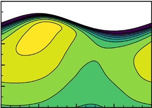
Figure 3 shows the contours of the phase-averaged Reynolds normal stresses $\langle {u'^2_i}\rangle$ as defined by (A 1) for case 1 (${{La}}_t=0.35$) and case 3 (${{La}}_t=0.9$), which represent the scenarios of strong and weak wave forcing, respectively. The intensities of the turbulence fluctuations in the three directions are considerably different between the two cases. The streamwise Reynolds normal stress $\langle {u'^2}\rangle$ in case 1 is much weaker than that in case 3, indicating that the streamwise velocity fluctuations are suppressed in strong Langmuir turbulence. Meanwhile, $\langle {v'^2}\rangle$ and $\langle {w'^2}\rangle$ are increased as the wave forcing becomes stronger due to the enhanced streamwise vortical structures and the strong vertical mixing present in the Langmuir turbulence. With the suppression of $\langle {u'^2}\rangle$ and the intensification of $\langle {v'^2}\rangle$ and $\langle {w'^2}\rangle$, the vertical and spanwise fluctuations become significantly stronger than the streamwise fluctuations in case 1. On the other hand, case 3 with the weak wave forcing has the relation $\langle {u'^2}\rangle >\langle {v'^2}\rangle >\langle {w'^2}\rangle$, similar to the turbulent flow driven by shear only. The above results indicate that the anisotrophy of the turbulence in case 1 is mainly caused by the wave. Our numerical results are consistent with the observations of the Langmuir turbulence in the literature (McWilliams et al. Reference McWilliams, Sullivan and Moeng1997; D'Asaro Reference D'Asaro2001; Li et al. Reference Li, Garrett and Skyllingstad2005), further confirming that the wave-phase-resolved LES successfully captures the effect of wave forcing and the features of Langmuir turbulence.

Figure 3. Contours of phase-averaged Reynolds normal stresses (a,d) $\langle {u'^2}\rangle$, (b,e) $\langle {v'^2}\rangle$ and (c,f) $\langle {w'^2}\rangle$ for (a–c) case 1 (${{La}}_t=0.35$) and (d–f) case 3 (${{La}}_t=0.9$), respectively. The Reynolds stresses are normalized by $u_*^2$. The grey lines in (a) represent the fixed depth $kz=-0.1$ (— $\cdot$ —) and the Lagrangian trajectory with a mean depth $kz=-0.1$ (– – –) that are used in figures 5 and 6, respectively.

In the vertical direction both horizontal velocity fluctuations, $\langle {u'^2}\rangle$ and $\langle {v'^2}\rangle$, increase towards the free surface. This is expected because the wave and current forcing that provide energy to the turbulence is stronger near the surface. Meanwhile, the kinematic blocking effect of the free surface leads to the energy redistribution from the vertical turbulence fluctuations to the horizontal components, which also increases the energy of $\langle {u'^2}\rangle$ and $\langle {v'^2}\rangle$ (Shen et al. Reference Shen, Zhang, Yue and Triantafyllou1999; Guo & Shen Reference Guo and Shen2010, Reference Guo and Shen2014). Also due to the blocking effect, $\langle {w'^2}\rangle$ decreases as the free surface is approached. We can also see from figure 3 that the contours of $\langle {u'^2_i}\rangle$ near the wave surface follow the wave geometry closely in case 1 (${{La}}_t=0.35$) and roughly in case 3 (${{La}}_t=0.9$). This result indicates that the intensity of near-surface turbulence fluctuations is dependent on the vertical distance from the wave surface. This surface effect can extend to approximately $k(z-\eta )=-0.2$ for $\langle {u'^2}\rangle$ and $\langle {w'^2}\rangle$ and $k(z-\eta )=-0.7$ for $\langle {v'^2}\rangle$ (whole range not plotted). In the following § 3.2 the effect of the vertical variation of the turbulence intensity on the wave-phase variation of Reynolds stresses is further discussed.

The phase-averaged Reynolds shear stress $\langle {-u'w'}\rangle$ for case 1 (${{La}}_t=0.35$) and case 3 (${{La}}_t=0.9$) are shown in figures 4(a) and 4(b), respectively. The shear stress in case 1 is stronger than that in case 3, indicating that the momentum transport in the vertical direction is enhanced by the wave forcing, as expected from the increased $\langle {w'^2}\rangle$ discussed above. The greater momentum mixing leads to a more uniform profile of the mean current in Langmuir turbulence (see, e.g. Xuan et al. Reference Xuan, Deng and Shen2019). We can see from figure 4 that the influence of the wave phase is obvious for the Reynolds shear stress, which is quantified in the following § 3.2. In the vicinity of the surface the shear stress decreases rapidly in both cases due to the constraint imposed by the surface blocking effect. However, we shall note that the values of $\langle {-u'w'}\rangle$ do not go to zero at the surface, for which the reason is discussed in the following section.

Figure 4. Contours of phase-averaged Reynolds shear stress $\langle {-u'w'}\rangle$ for (a) case 1 (${{La}}_t=0.35$) and (b) case 3 (${{La}}_t=0.9$). The stress is normalized by $u_*^2$.

3.2. Wave-phase variation of Reynolds stresses

As discussed in § 3.1 and shown in figure 3, the near-surface intensity of the turbulence velocity fluctuations is affected by the distance from the wave surface. In other words, if the turbulence statistics are measured at a fixed location, especially near the surface, they are expected to vary with the wave phase due to the passage of the wave. We take the streamwise Reynolds stress $\langle {u'^2}\rangle$ as an example. Figure 5 plots the variation of $\langle {u'^2}\rangle$ at the location $kz=-0.1$ along with the data from the laboratory measurements of the turbulence under a wind-sheared surface wave by Jiang & Street (Reference Jiang and Street1991) and Thais & Magnaudet (Reference Thais and Magnaudet1996). These experiments are estimated to have comparable ${{La}}_t$ with case 2 in our study. The LES result shows that the maximum $\langle {u'^2}\rangle$ occurs under the wave trough. This is because $\langle {u'^2}\rangle$ increases as the surface is approached (figure 3a) and the distance to the surface is the shortest under the wave trough. We shall note that, for other cases considered in this study, the phase variation of $\langle {u'^2}\rangle$ is qualitatively similar but has different magnitudes due to different vertical variations of the streamwise fluctuations. For example, case 1 (${{La}}_t=0.35$) is found to have a larger variation of $\langle {u'^2}\rangle$ than case 2, mostly because the intensity of $\langle {u'^2}\rangle$ increases more sharply near the surface. When comparing the numerical result with the experiments, we can see that the phase variation of $\langle {u'^2}\rangle$ is consistent while the magnitude of the variation is slightly smaller than the experiments. The difference in the variation magnitude could be caused by the fact that the experimental conditions and our idealized simulation set-up are not matched exactly. For example, in the experiment by Jiang & Street (Reference Jiang and Street1991) with $U_{{air}}=2.5\ \text {m}\ \text {s}^{-1}$ in the wind–wave tank, a return Eulerian flow with negative velocity is present at the water bottom and, therefore, the profile of the mean current is different from our simulation set-up. This can lead to a different vertical distribution of turbulent kinetic energy and, thus, the difference in the variation magnitude of $\langle {u'^2}\rangle$. Other factors, such as the wind–wave coupling, may also lead to discrepancies between our simulation and the experiments. Despite that the experimental data have more fluctuations than the simulation result, their overall agreement is encouraging.

Figure 5. Normalized variation of Reynolds normal stress $\langle {u'^2}\rangle$ at the fixed depth $kz=-0.1$ in case 2 (——). The values of $\langle {u'^2}\rangle$ are normalized by its mean value over the wave period at that depth, $\overline {u'^2}={(L_x)}^{-1}\int _{0}^{L_x} \langle {u'^2}\rangle \,\mathrm {d}x$. The experimental data plotted in the figure for comparison are from: Jiang & Street (Reference Jiang and Street1991) with an air speed $U_{air}=2.5\ \mathrm {m}\ \mathrm {s}^{-1}$ and an estimated turbulent Langmuir number ${{La}}_t=0.52$ ($\vartriangle$); Jiang & Street (Reference Jiang and Street1991) with $U_{air}=4.1\ \mathrm {m}\ \mathrm {s}^{-1}$ and ${{La}}_t=0.66$ ($\square$); Thais & Magnaudet (Reference Thais and Magnaudet1996) with $U_{air}=4.5\ \mathrm {m}\ \mathrm {s}^{-1}$ and ${{La}}_t=0.57$ (case E2) (${\Large \circ }$). The wave surface geometry $\eta$ corresponding to the wave phase $kx$ is illustrated using the solid line above the plot. The dotted line with the arrow above the plot indicates that the variation is measured at a fixed depth (the dash–dotted line in figure 3a) and the phase change is in the ${-}x$-direction in the wave-following frame.

However, relying on the observation at a fixed point has the shortcoming of failing to account for the region between the wave trough and the wave crest. To overcome this drawback, we instead consider the variation of the turbulence statistics along the Lagrangian trajectory of a fluid element convected by the wave, i.e. along the streamline of the mean flow in the wave-following frame. As illustrated in figure 2, the streamline follows the wave surface geometry such that the region below the wave crest is included. Moreover, as discussed above, the variation of Reynolds normal stresses at a fixed point is mainly due to the kinematic motion, i.e. the change of the distance from the surface. By contrast, the Lagrangian trajectory follows the wave geometry and, thus, reflects the variation of turbulence statistics due to flow dynamics more closely.

Figure 6 plots the normalized variation of the Reynolds normal stresses, ${({u'^2_i})}^l/{\overline {u'^2_i}}^L$. By definition (A 3), ${({u'^2_i})}^l$ reflects the variation of $\langle {u'^2_i}\rangle$ along the streamline of the wave in the wave-following frame. Also plotted is the theoretical prediction of the wave-phase variation of the streamwise and vertical Reynolds normal stresses based on the RDT analysis by Teixeira & Belcher (Reference Teixeira and Belcher2002), which is given by

(3.1a)\begin{gather} \frac{{(u'^2)}^l}{{\overline{u'^2}}^L} = \frac{4}{5} ak \,\textrm{e}^{kz} \sin (kx-\sigma t), \end{gather}

(3.1b)\begin{gather}\frac{{(w'^2)}^l}{{\overline{w'^2}}^L} = - \frac{4}{5} ak \,\textrm{e}^{kz} \sin (kx-\sigma t). \end{gather}

We note that the above prediction is obtained from a simplified RDT model which considers only the normal straining of the wave, i.e. ${\partial } u_w/{\partial } x$ and ${\partial } w_w/{\partial } z$. Teixeira & Belcher (Reference Teixeira and Belcher2002) found that considering only the normal straining can yield a good approximation of the full RDT model with all components of the straining in terms of the fluctuating amplitude and phase distribution, and, therefore, neglected the effects of the shear straining. In the mean time, with only the normal straining, the model for slab-symmetric straining flows (Townsend Reference Townsend1998) can be employed to obtain explicit expressions for the evolution of Reynolds stresses. Therefore, the simplified model is used here for comparisons with our LES results. For the spanwise Reynolds stress, the simplified RDT model yields a result that depends on the initial condition and is thus not suitable for the comparison with the quasi-steady flow in the present work.

Figure 6. Normalized wave-phase variation of Reynolds normal stresses in the wave-following frame along the Lagrangian trajectory with a mean depth $kz=-0.1$ for case 1 (——), case 2 (– – –), case 3 (— $\cdot$ —) and case 1S (— $\cdot$$\cdot$ —): (a) ${(u'^2)}^l/{\overline {u'^2}}^L$, (b) ${(v'^2)}^l/{\overline {v'^2}}^L$ and (c) ${(w'^2)}^l/{\overline {w'^2}}^L$. For comparison, the theoretical results (3.1) based on the RDT analysis by Teixeira & Belcher (Reference Teixeira and Belcher2002) for $ak=0.084$ ($\vartriangle$) and $ak=0.15$ (${\Large \circ }$) are plotted. The wave surface geometry $\eta$ corresponding to the wave phase $kx$ is illustrated using the solid line above the plot. The dotted line with the arrows above the plot indicates that the variation is measured following the Lagrangian trajectory (the dashed line in figure 3a), which points to the ${-}x$-direction in the wave-following frame.

As shown in figure 6(a), the values of ${({u'^2})}^l$ for different simulation cases vary sinusoidally with the wave phase. The maxima and minima of ${({u'^2})}^l$ indicate that, along the streamline, $\langle {u'^2}\rangle$ is stronger under the crest and weaker under the trough, respectively. This distribution is roughly consistent with the prediction by the RDT analysis (3.1a). The magnitude of ${({u'^2})}^l$ also shows an overall agreement with the theoretical model, which predicts that the magnitude of the variation of $\langle {u'^2}\rangle$ is proportional to the wave steepness $ak$. These results indicate that the simplified RDT model (3.1a) can capture the dominant dynamics underlying the wave-phase variation of $\langle {u'^2}\rangle$. However, we also find that the extrema of $\langle {u'^2}\rangle$ deviate slightly from the crest or trough because (3.1a) considers only the normal straining. The neglected processes, such as the shear straining, can lead to the phase shift of the Reynolds stresses. Nevertheless, the maximum deviation among all the cases at all depths is within $12^{\circ }$ (not plotted), indicating that the normal straining governs the wave-phase variation of the streamwise stress, which is also shown in the analysis of budgets in § 3.3.

The trajectory-following result shown in figure 6(a) is completely different from the fixed-point result (figure 5), suggesting that the kinematic-induced fluctuation of $\langle {u'^2}\rangle$ is indeed dominant in the fixed-point observation and this effect is removed in the Lagrangian approach. This contrast suggests that care should be taken when interpreting data from fixed-point measurement under water waves, as one would obtain from experiments. To remove the kinematics-induced fluctuations from fixed-point observations, a coordinate transformation can be performed to obtain the Lagrangian fluctuations of turbulence statistics. For a trajectory, the vertical deviation of its mean depth, $\xi ^3$ (see appendix A), can be approximated using a linear relation as

(3.2)\begin{equation} \xi^3 = \textrm{e}^{kz} \langle {\eta}\rangle, \end{equation}

where $z$ is the mean depth of the trajectory. Then, using the above coordinate transformation, the turbulence statistics along the Lagrangian trajectory can be computed by interpolating the fixed-point data at each wave phase onto the location of the trajectory, $z+\xi ^3$.

The spanwise Reynolds normal stress also exhibits a sinusoidal variation with the wave phase (figure 6b). The value of ${({v'^2})}^l$ reaches its maxima near the wave trough and on the backward slope, and reaches its minima on the forward slope side of the wave crest. This behaviour is consistent with the wave-phase variation of the streamwise component of the enstrophy $\langle {\omega _x^2}\rangle$, whose maximum and minimum values are ahead of the wave trough and crest, respectively (Xuan et al. Reference Xuan, Deng and Shen2019). The connection between the wave-phase distributions of ${({v'^2})}^l$ and ${\omega _x^2}$ is not surprising because the enhanced spanwise turbulence fluctuations in Langmuir turbulence are associated with the elongated streamwise vortical structures.

The variation of the vertical Reynolds stress ${({w'^2})}^l$ observed in our simulation is different from the RDT prediction (3.1b), as shown in figure 6(c). Our result shows that the variation of ${({w'^2})}^l$ with the wave phase is much weaker compared with the horizontal Reynolds stresses, indicating a weak modulation of the wave phase on the vertical velocity fluctuations. On the other hand, the RDT theory predicts the fluctuation magnitude of ${({w'^2})}^l$ to be as strong as that of ${({u'^2})}^l$. The above results show that the turbulence intensities are indeed affected by the direct wave distortion. However, the existing theoretical model based on the RDT cannot fully explain the observed behaviours. Later through the analyses of the budget balance of $\langle {u'^2_i}\rangle$ in § 3.3, we show that the discrepancy between our numerical results and the RDT prediction is related to the turbulence-pressure-related effects.

Next, we discuss the wave-phase variation of the Reynolds shear stress. The Lagrangian fluctuation ${(u'w')}^l$ of $kz=-0.2$ is shown in figure 7(a). The maximum shear stress occurs under the wave crest, indicating that the momentum transport is enhanced under the crest. This result is consistent with the findings by Thais & Magnaudet (Reference Thais and Magnaudet1996), who observed from their experiments that the turbulence bursting events are more pronounced under the wave crest. The RDT analysis of the temporal evolution of an initially isotropic turbulence (Teixeira & Belcher Reference Teixeira and Belcher2002, figure 9) also shows that the maxima of the Reynolds shear stress occur under the wave crest after a few wave periods. We also note that the fluctuation magnitude of the shear stress clearly relates to the wave steepness because the variation of ${({u'w'})}^l$ is similar for cases 1–3 but larger for case 1S.

Figure 7. Normalized wave-phase variation of Reynolds shear stress in the wave-following frame for case 1 (——), case 2 (– – –), case 3 (— $\cdot$ —) and case 1S (— $\cdot$$\cdot$ —): (a) ${(u'w')}^l/{\overline {u'w'}}^L$ along the Lagrangian trajectory with a mean depth $kz=-0.1$ and (b) ${(u'w')}^l/{\overline {u'^2}}^L$ at the surface. In (b) the approximation (3.4) is plotted for $ak=0.084$ ($\vartriangle$) and $ak=0.15$ (${\Large \circ }$).

At the surface, a different variation of ${({u'w'})}^l$ is observed as shown in figure 7(b). We find that the variation of $u'$ and $w'$ is governed by the surface blocking effect. Because the direction of the velocity fluctuations are constrained by the inclined wave surface, the velocity at the surface approximately satisfies

(3.3)\begin{equation} w' \approx u' \eta_x,\quad \text{at } z=\eta. \end{equation}

This leads to

(3.4)\begin{equation} u'w' \approx u'^2 \eta_x,\quad \text{at } z=\eta. \end{equation}

The wave-phase variation of ${({u'w'})}^l$ is well described by (3.4), as shown in figure 7(b). In other words, $u'$ and $w'$ are positively and negatively correlated under the backward and forward slope, respectively. However, we shall note that the kinematic-induced $u'w'$ does not contribute to the dynamics of momentum mixing, as the viscous effect dominates the momentum transport near the boundary. This is consistent with the fact that ${\overline {u'w'}}^L$ is approximately zero at the surface. It is later discussed in § 4 that the wave-phase fluctuation of $\langle {u'w'}\rangle$ away from the surface, where the extrema of it are under the wave crest and trough, can influence the dynamics of TKE. On the other hand, the wave-phase variation of $\langle {u'w'}\rangle$ induced by the blocking effect at the surface has no contribution to the TKE dynamics (§ 4.3).

3.3. Reynolds stress budget in the wave-phase-resolved frame

To explain the mechanism underlying the variation of Reynolds stresses with the wave phase shown in § 3.2, we next analyse the budget of the Reynolds stresses in the wave-following frame. Using the definition of the phase averaging $\langle {\cdot }\rangle$ (A 1), we can obtain the evolution equation for the phase-averaged resolved Reynolds stress $\langle {u'_i u'_j}\rangle$,

(3.5)\begin{equation} \frac{\mathrm{D} \langle {u'_i u'_j}\rangle}{\mathrm{D} t} = \frac{{\partial} \langle {u'_i u'_j}\rangle}{{\partial} t} + (\langle {\boldsymbol{u}}\rangle-c)\boldsymbol{\cdot} \boldsymbol{\nabla}\langle {u'_i u'_j}\rangle = P^c_{ij} + P^w_{ij} + {\varPi}_{ij} + T^t_{ij} + \epsilon_{ij}. \end{equation}

Here, owing to the quasi-steadiness of the flow, ${\partial } \langle {u'_i u'_j}\rangle /{\partial } t$ is approximately zero and, thus, the material derivative ${\mathrm {D} \langle {u'_i u'_j}\rangle }/{\mathrm {D} t} \approx (\langle {\boldsymbol {u}}\rangle -c)\boldsymbol {\cdot }\boldsymbol {\nabla }\langle {u'_i u'_j}\rangle$ represents the change rate of Reynolds stresses under the advection of $\langle {\boldsymbol {u}}\rangle -c$, i.e. the wave-phase variation of Reynolds stresses. Note that the wave phase speed $c$ appears owing to the translation of the observation frame. The terms on the right-hand side of (3.5) represent different processes contributing to the wave-phase variation of $\langle {u'_i u'_j}\rangle$, corresponding to the positive–negative fluctuations of $\mathrm {D} \langle {u'_i u'_j}\rangle /\mathrm {D} t$ with the wave phase. The first two terms, $P^c_{ij}$ and $P^w_{ij}$, defined as

(3.6)\begin{gather} P^c_{ij} = -\langle {u'_i u'_k}\rangle\frac{{\partial} {(u_c)}_j}{{\partial} x_k}-\langle {u'_j u'_k}\rangle\frac{{\partial} {(u_c)}_i}{{\partial} x_k}, \end{gather}

(3.7)\begin{gather}P^w_{ij} = -\langle {u'_i u'_k}\rangle\frac{\partial{{(u_w)}_j}}{\partial{x_k}}-\langle {u'_j u'_k}\rangle\frac{\partial{{(u_w)}_i}}{\partial{x_k}}, \end{gather}

represent the production of $\langle {u'_i u'_j}\rangle$ caused by the straining of the mean current and wave, respectively. As the wave straining has both the normal and shear straining, $P^w_{ij}$ can be contributed by the interaction between the normal stress and normal straining, namely the normal production, and the interaction between the shear stress and shear straining, namely the shear production. The velocity–pressure-gradient term $\varPi _{ij}$ is defined as

(3.8)\begin{equation} \varPi_{ij} = -\frac{1}{\rho}\left\langle {u'_i \frac{\partial{p'}}{\partial{x_j}}+u'_j \frac{\partial{p'}}{\partial{x_i}}}\right\rangle. \end{equation}

The term $T^t_{ij}$ is defined as

(3.9)\begin{equation} T^t_{ij} = -\frac{\partial{\langle {u'_k u'_i u'_j}\rangle}}{\partial{x_k}}-\frac{\partial{\langle{u'_i\tau'_{jk}}\rangle}}{\partial{x_k}} -\frac{\partial{\langle{u'_j\tau'_{ik}}\rangle}}{\partial{x_k}} + \nu\nabla^2{\langle {u'_i u'_j}\rangle}. \end{equation}

This term represents the change of $\langle {u'_i u'_j}\rangle$ caused by the spatial fluxes driven by the resolved turbulence, the SGS turbulence and the viscous diffusion. The last term in (3.5), $\epsilon _{ij}$, is the dissipation associated with the resolved-scale and SGS turbulence, defined as

(3.10)\begin{equation} \epsilon_{ij} = -2\nu\left\langle \frac{\partial{u'_i}}{\partial{x_k}}\frac{\partial{u'_j}}{\partial{x_k}} \right\rangle + \left\langle {\tau'_{ik}\frac{\partial{u'_j}}{\partial{x_k}}}\right\rangle +\left\langle {\tau'_{jk}\frac{\partial{u'_i}}{\partial{x_k}}}\right\rangle. \end{equation}

The velocity–pressure-gradient term $\varPi _{ij}$ (3.8) can be decomposed into the pressure transport term $T^p_{ij}$ and pressure–strain correlation term $R_{ij}$,

(3.11)\begin{equation} \varPi_{ij} = T^p_{ij} + R_{ij}, \end{equation}

where

(3.12)\begin{gather} T^p_{ij} = -\frac{1}{\rho} \left(\frac{\partial{\langle {p'u'_i}\rangle}}{\partial{x_j}} + \frac{\partial{\langle {p'u'_j}\rangle}}{\partial{x_i}}\right), \end{gather}

(3.13)\begin{gather}R_{ij} = \left\langle {\frac{p'}{\rho} \left(\frac{\partial{u'_i}}{\partial{x_j}} + \frac{\partial{u'_j}}{\partial{x_i}}\right)}\right\rangle. \end{gather}

The pressure transport term $T^p_{ij}$ represents the spatial transport rate of the Reynolds stresses by turbulent pressure fluctuations. The sum of the normal pressure–strain correlation $R_{ii}$ is zero because of the incompressibility, i.e. the pressure–strain correlation is associated with the inter-component energy transfer among the three Reynolds normal stresses. We note that the decomposition of the velocity–pressure-gradient term is not unique (Lumley Reference Lumley1975; Pearson et al. Reference Pearson, Grant and Polton2019). The adopted decomposition has been widely used for studying turbulence dynamics (see, e.g. Speziale, Sarkar & Gatski Reference Speziale, Sarkar and Gatski1991; Harcourt Reference Harcourt2013).

The Reynolds stress budget equations in the wave-phase-resolved frame (3.5) differ from those derived from the CL models (see, e.g. Harcourt Reference Harcourt2013) in that the wave velocity $\boldsymbol {u}_w$ appears explicitly in the budget terms. To be specific, the advection term, $(\boldsymbol {u}-c)\boldsymbol {\cdot }\boldsymbol {\nabla }\langle {u'_i u'_j}\rangle$, includes the orbital motions of the wave as it represents the wave-phase variation of Reynolds stresses. The production terms $P^w_{ij}$ also relate directly to the velocity gradients of the wave motions rather than the Stokes drift so that $P^w$ can account for the effect of wave phases. The remaining terms have similar expressions with those in the CL-based equations.

As discussed above, the variations of Reynolds stresses with the wave phase observed in § 3.2 correspond to the positive–negative fluctuations of $\mathrm {D}\langle {u'_i u'_j}\rangle /\mathrm {D}t$, which we find are mostly caused by the production by the wave, $P^w$, and the velocity–pressure-gradient term, $\varPi$. These two terms exhibit nearly sinusoidal variations with the wave phase. As a result, Reynolds stresses are increased and decreased under different phases, leading to their variations with the wave phase. By comparison, the fluctuations of the remaining terms are at least one order of magnitude in $ak$ weaker and, thus, have negligible contributions to the fluctuations of $\mathrm {D}\langle {u'_i u'_j}\rangle /\mathrm {D}t$. This indicates that the wave-phase variation of the Reynolds stresses is governed by $P^w$ and $\varPi$. The Reynolds stress budgets for different cases considered in this study are qualitatively similar; therefore, case 1 is used here as a representative for the explanation of the mechanisms of the wave-phase variation of the Reynolds stresses.

We first discuss the physical processes of the wave-phase variation of the streamwise Reynolds normal stress $\langle {u'^2}\rangle$. To reveal the inter-component energy transfer for the Reynolds normal stresses, we apply the decomposition (3.12) and (3.13) to $\varPi _{ii}$ for all three components of Reynolds normal stresses. Figure 8 shows the contours of $P^w_{xx}$, $T^p_{xx}$ and $R_{xx}$, with the production $P^w_{xx}$ decomposed into the normal production $-2\langle {u'^2}\rangle {\partial } u_w/{\partial } x$ (figure 8a) and the shear production $-2\langle {u'w'}\rangle {\partial } u_w/{\partial } z$ (figure 8b). Among these terms, the normal production is dominant and contributes the most to the wave-phase variation of $\langle {u'^2}\rangle$. Under the wave forward slope, ${\partial } u_w/{\partial } x$ is negative (figure 2b) and the resulting normal production is positive, indicating that $\langle {u'^2}\rangle$ gains energy from the streamwise compression of the wave motions. The opposite process occurs under the backward slope. Towards the wave surface, with the increase of $\langle {u'^2}\rangle$ (figure 3a) and the velocity gradient ${\partial } u_w/{\partial } x$, the rate of the energy exchange between $\langle {u'^2}\rangle$ and the wave through the normal production also increases. Because the convection by the wave is in the ${-}x$-direction relative to the frame moving with the wave, the alternating enhancement and suppression of the $\langle {u'^2}\rangle$ result in maximal $\langle {u'^2}\rangle$ under the wave crest and minimal under the wave trough, consistent with figure 6(a). Finally, because the RDT theory also assumes that the straining effect is the dominant mechanism for the rapid distortion of the turbulence, the wave-phase variation of $\langle {u'^2}\rangle$ is well predicted by the RDT theory (3.1a), as shown in § 3.2. In the budget equation of $\langle {v'^2}\rangle$, the production and pressure transport are both zero according to the definition of phase averaging (A 1). The pressure–strain correlation $R_{yy}$ shown in figure 9 is the dominant term in the budget of $\langle {v'^2}\rangle$. The value of $R_{yy}$ is positive and negative under the wave backward and forward slope, respectively. As a result, $\langle {v'^2}\rangle$ is enhanced when the wave backward slope passes and is weakened when the forward slope passes, consistent with the wave-phase variation of ${({v'^2})}^l$ shown in § 3.2 (figure 6b). We also note that $R_{ii}$ represents the inter-component energy transfer, which means that the wave-phase variation of $\langle {v'^2}\rangle$ is not directly affected by the wave straining but is sustained by its periodic energy exchange with the other two components of the Reynolds normal stresses (mostly $\langle {w'^2}\rangle$ as discussed below). Figure 10 shows the dominant terms in the budget of $\langle {w'^2}\rangle$. Among these terms, the shear production (figure 10b) is significantly weaker, therefore, the weak wave-phase variation of $\langle {w'^2}\rangle$ (figure 6c) results from the balance among the normal production (figure 10a), the pressure transport (figure 10c) and the pressure–strain correlation (figure 10d). The normal production $-2\langle {w'^2}\rangle {\partial } w_w/{\partial } z$ is negative and positive under the forward and backward slopes, respectively. Meanwhile, the phase distribution of the pressure–strain correlation $R_{zz}$, i.e. positive under the forward slope and negative under the backward slope, is opposite to that of the normal production. The pressure transport $T^p_{zz}$ relating to the diffusion of $\langle {w'^2}\rangle$ due to the turbulence pressure in the vertical direction has a two-layer structure, as shown in figure 10(c). Under the forward slope, $T^p_{zz}$ is negative near the surface and becomes positive away from the surface, indicating that the energy of $\langle {w'^2}\rangle$ is transported from the surface to the deep region. The energy transport direction reverses under the backward slope, i.e. from the deep region to the surface. Comparing the magnitude of the above three terms, we can now explain their net effect on $\langle {w'^2}\rangle$. Under the forward slope, the energy gained through the positive pressure–strain correlation near the surface overweights the negative normal production. The excess of the energy is removed from the near-surface region and transported to the deep region through the pressure transport. Similarly, under the backward slope, the pressure fluctuations transports energy from the deep region to the surface and compensates the difference between the pressure–strain correlation and the normal production. As a result of the balance described above, the strength of $\langle {w'^2}\rangle$ changes little with the wave phase. By comparison, in the RDT model, the normal straining is assumed to be the dominant mechanism for the wave-phase variation of the Reynolds stresses. If we consider the normal production only (figure 10a), the maxima and minima of $\langle {w'^2}\rangle$ would be under the wave trough and crest, respectively, as predicted by the RDT model (3.1b). This suggests that the effects of the turbulence pressure, including the pressure transport and pressure–strain correlation, are not fully accounted for by the RDT model.

Figure 8. Contours of the dominant budget terms of $\langle {u'^2}\rangle$, including the production due to the wave $P^w_{xx}$, (a) $-2\langle {u'^2}\rangle {\partial } u_w/{\partial } x$ and (b) $-2\langle {u'w'}\rangle {\partial } u_w/{\partial } z$, (c) the pressure transport $T^p_{xx}$ and (d) the pressure–strain correlation $R_{xx}$. The results are normalized by $u_*^2 ak\sigma$.

Figure 9. Contours of the dominant budget term of $\langle {v'^2}\rangle$, pressure–strain correlation $R_{yy}$. The results are normalized by $u_*^2 ak\sigma$.

Figure 10. Contours of the dominant budget terms of $\langle {w'^2}\rangle$, including the production due to the wave $P^w_{zz}$, (a) $-2\langle {w'^2}\rangle {\partial } w_w/{\partial } z$ and (b) $-2\langle {u'w'}\rangle {\partial } w_w/{\partial } x$, (c) pressure transport $T^p_{zz}$ and (d) pressure–strain correlation $R_{zz}$. The results are normalized by $u_*^2 ak\sigma$.

We can see from the above analyses that the terms related to the turbulence pressure play an important role in the wave-phase variation of the Reynolds normal stresses. Specifically, the dynamics of $\langle {v'^2}\rangle$ and $\langle {w'^2}\rangle$ are closely related to the pressure–strain correlation $R_{ii}$. We notice that the magnitude of $R_{zz}$ (figure 10d) is approximately the same as $R_{yy}$ (figure 9), indicating that the inter-component energy exchange occurs mainly between $\langle {v'^2}\rangle$ and $\langle {w'^2}\rangle$. The energy transfers from $\langle {w'^2}\rangle$ to $\langle {v'^2}\rangle$ under the backward slope and then transfers back under the forward slope. The sign-alternating variation of the pressure–strain correlation can be explained by the blocking effect of the wave surface (Guo & Shen Reference Guo and Shen2014). As the fluid elements move under the backward slope, the decreased surface elevation compresses the fluid elements in the vertical direction. As a result, the fluid elements move closer to the surface and experience the blocking effect of the surface. As the vertical turbulence fluctuations are restricted by the surface blocking, the energy transfers from $\langle {w'^2}\rangle$ to $\langle {v'^2}\rangle$. Under the forward slope, as the surface elevation increases, the reverse process occurs.

To summarise the mechanisms of the wave-phase variation of the Reynolds normal stresses $\langle {u'^2_i}\rangle$, we sketch the dominant processes in the budget of $\langle {u'^2_i}\rangle$ in figure 11. The wave-phase variation of $\langle {u'^2}\rangle$ is mainly associated with its direct energy exchange with the wave through the wave normal production, resulting in the maximum of $\langle {u'^2}\rangle$ under the wave crest and minimum under the trough. The wave-phase variation of $\langle {v'^2}\rangle$ is caused by its energy exchange with $\langle {w'^2}\rangle$ through the pressure–strain correlation, which increases $\langle {v'^2}\rangle$ under the backward slope and reduces $\langle {v'^2}\rangle$ under the forward slope. The effects of the pressure–strain correlation are related to the strengthening and weakening of the blocking effect of the water surface due to the undulating motions of the wave. Lastly, the energy gain or loss of $\langle {w'^2}\rangle$ with $\langle {v'^2}\rangle$ through the pressure–strain correlation is balanced with the wave normal production and the pressure transport. The net effect of these three processes results in the weak wave-phase variation of $\langle {w'^2}\rangle$. We note that, although there is no direct interaction between $\langle {v'^2}\rangle$ and the wave straining through the production effect, $\langle {w'^2}\rangle$ acts as a conduit of energy exchange between $\langle {v'^2}\rangle$ and the wave.

Figure 11. Sketch of the dominant processes contributing to the wave-phase variation of the Reynolds normal stresses. The arrows indicate the direction of the energy flux. The solid arrows represent the wave normal production. The arrows with dash–dotted lines represent the pressure transport. The hollow arrows with dash–dot–dot lines indicate the pressure–strain correlation.

Next, we analyse the budget of the Reynolds shear stress $-\langle {u'w'}\rangle$. Because the variation of $\langle {u'w'}\rangle$ at the surface is due to the surface kinematics as discussed in § 3.2, here we focus on the processes occurring away from the surface, where $-\langle {u'w'}\rangle$ obtains its maxima under the crest and minima under the trough (figure 7a in § 3.2). Note that for the Reynold shear stress, if we apply the decomposition (3.11) to the velocity–pressure-gradient terms, there are two pressure transport terms $R_{xz}$ (3.12) and two pressure–strain correlation terms $T^p_{xz}$ (3.13), which complicates the analyses. Therefore, we keep the form of the velocity–pressure-gradient terms, $-\langle {u'{\partial } p'/{\partial } z}\rangle$ and $-\langle {w'{\partial } p'/{\partial } x}\rangle$, to facilitate the analysis of the wave-phase variation of $\langle {u'w'}\rangle$.

Figure 12 shows the contours of the production terms (figures 12a and 12b) and the velocity–pressure-gradient terms (figures 12c and 12d). Note that the budget equation (3.5) has been multiplied by $-1$ such that these terms represent the variation of $-\langle {u'w'}\rangle$. The two production terms represent the generation of $\langle {u'w'}\rangle$ from the shear straining of the normal velocity fluctuations $\langle {u'^2}\rangle$ and $\langle {w'^2}\rangle$. We can see that all the four terms exhibit obvious wave-phase variation, indicating the complicated physical processes involved with the Reynolds shear stress. Upon a closer examination, we find that the production associated with the vertical normal stress $\langle {w'^2}\rangle {\partial } w_w/{\partial } x$ (figure 12b) can roughly cancel the pressure term associated with the vertical velocity fluctuation $\langle {w'{\partial } p'/{\partial } x}\rangle$ in most of the region. To illustrate their net effect, the sum of the these two terms is plotted in figure 12(e), from which we can see that its wave-phase variation is much weaker than the two individual terms. When we compare figure 12(e) with figures 12(a) and 12(c), we can now see clearly that the pressure effect term $\langle {u' {\partial } p'/{\partial } z}\rangle$ overwhelms the other terms and is the dominant mechanism that determines the wave-phase variation of the shear stress. For example, in the ${-}x$-direction, the value of $\langle {u' {\partial } p'/{\partial } z}\rangle$ changes from positive to negative near the wave crest, which means that $\langle {u' {\partial } p'/{\partial } z}\rangle$ alone would lead to the maxima of $-\langle {u'w'}\rangle$ approximately under the wave crest. Meanwhile, the production term $\langle {u'^2}\rangle {\partial } w_w/{\partial } x$ (figure 12a) and the summed term (figure 12e) offset $\langle {u' {\partial } p'/{\partial } z}\rangle$ and shift the positive and negative regions of $\langle {u' {\partial } p'/{\partial } z}\rangle$ further towards the ${-}x$-direction, which results in the maxima and minima of $-\langle {u'w'}\rangle$ under the wave crest and trough, respectively (figure 4 in § 3.2). From the above analyses we can see that the turbulence pressure is not only important to the dynamics of the Reynolds normal stresses $\langle {v'^2}\rangle$ and $\langle {w'^2}\rangle$, but also plays a crucial role in the wave-phase variation of the Reynolds shear stress $-\langle {u'w'}\rangle$.

Figure 12. Contours of the dominant terms in the evolution equation of $-\langle {u'w'}\rangle$: (a) $\langle {u'^2}\rangle {\partial } w_w/{\partial } x$, (b) $\langle {w'^2}\rangle {\partial } u_w/{\partial } z$, (c) $\langle {u' {\partial } p'/{\partial } z}\rangle$, (d) $\langle {w' {\partial } p'/{\partial } x}\rangle$ and (e) $\langle {w'^2}\rangle {\partial } u_w/{\partial } z+ \langle {w' {\partial } p'/{\partial } x}\rangle$.

4.1. Lagrangian-averaged TKE budget

The budget equation of the Lagrangian-averaged TKE ${\bar {E}}^L$, where $E=u_i'u_i'/2$, is

(4.1)\begin{equation} \frac{{\bar{\mathrm{D}}}^L {\bar{E}}^L}{\bar{\mathrm{D}} t} = {\overline{P^c}}^L + {\overline{P^w}}^L + {\overline{{T}^p}}^L + {\overline{T^t}}^L + {\bar{\epsilon}}^L, \end{equation}

which is obtained by summing up the budget equations of the three Reynolds normal stresses (3.5) and applying the Lagrangian average (A 2). Note that we have decomposed the velocity–pressure-gradient term into the pressure transport term $T^p_{ii}$ and the pressure–strain correlation term $R_{ii}$ as (3.11)–(3.13), and invoked the trace-free property of $R_{ii}$. Therefore, $R_{ii}$ that represents the inter-component energy transfer is cancelled among the three components of Reynolds normal stresses and only the pressure transport term appears in (4.1).

The terms on the right-hand side of (4.1) are the TKE production due to the sheared current ${\overline {P^c}}^L$,

(4.2)\begin{equation} {{\overline{P^c}}^L = -{\overline{{u' w'}\frac{{\partial} {u_c}}{{\partial} z}}}^L = -{\overline{u' w'}}^L\frac{{\partial} u_c}{{\partial} z}}, \end{equation}

the TKE production due to the wave straining ${\overline {P^w}}^L$,

(4.3)\begin{equation} {\overline{P^w}}^L = -{\overline{u'^2 \frac{\partial{u_w}}{\partial{x}}}}^L-{\overline{w'^2 \frac{\partial{w_w}}{\partial{z}}}}^L-{\overline{u'w' \frac{\partial{u_w}}{\partial{z}}}}^L-{\overline{u'w' \frac{\partial{w_w}}{\partial{x}}}}^L, \end{equation}

the diffusion of TKE due to the pressure fluctuations ${\overline {T^p}}^L$,

(4.4)\begin{equation} {\overline{T^p}}^L = -\frac{1}{\rho} \left({\overline{\frac{\partial{p'u'}}{\partial{x}}}}^L + {\overline{\frac{\partial{p'w'}}{\partial{z}}}}^L\right), \end{equation}

the diffusion due to the effects of the resolved turbulence fluctuations, SGS turbulence and viscosity ${\overline {T^t}}^L$,

(4.5)\begin{align} {\overline{T^t}}^L &= -{\overline{\frac{\partial{u' E}}{\partial{x}}}}^L-{\overline{\frac{\partial{w' E}}{\partial{z}}}}^L+ \nu{\overline{\nabla^2{E}}}^L \nonumber\\ &\quad -{\overline{\frac{\partial{({u'\tau'_{11}+v'\tau'_{12}+w'\tau'_{13}})}}{\partial{x}}}}^L -{\overline{\frac{\partial{({u'\tau'_{13}+v'\tau'_{23}+w'\tau'_{33}})}}{\partial{z}}}}^L, \end{align}

and the combined viscous and SGS dissipation ${\bar {\epsilon }}^L$,

(4.6)\begin{equation} {\bar{\epsilon}}^L = -\nu{\overline{\frac{\partial{u'_i}}{\partial{x_k}}\frac{\partial{u'_i}}{\partial{x_k}}}}^L+{\overline{\tau'_{ik}\frac{\partial{u'_i}}{\partial{x_k}}}}^L. \end{equation}

Note the in (4.2), ${\overline {u_c}}^L$ is equal to $u_c$ by definition (A 4).

To assess the characteristic features of the wave-phase-averaged budget of TKE, we focus on cases 1 and 3, representative of the strong (${{La}}_t=0.35$) and weak (${{La}}_t=0.9$) Langmuir turbulence, respectively. Their budget terms are plotted in figures 13(a) and 13(b), respectively. The deep bottom region is not plotted because our interest is the wave effect. In case 1 (figure 13a) the dominant source of the TKE is the production associated with the wave straining ${\overline {P^w}}^L$. The production due to the wave effect decays as the depth increases and becomes negligible compared to other terms at approximately $kz=-2$. The production by the current shear ${\overline {P^c}}^L$ as another source of the TKE is negligibly small except for close to the surface. This is because the Eulerian current is almost uniform away from the surface due to the enhanced mixing associated with the Langmuir turbulence, and only near the surface does the shear of the mean current become significant owing to the viscous effect. The dominance of the wave production is consistent with the findings from the CL model. In other words, the production by Stokes shear is the main source of TKE. For case 3 where the Langmuir turbulence is weak (figure 13b), the roles of the wave and current are reversed. In other words, because the strength of wave straining and the mixing due to the Langmuir circulations is relatively weak in case 3, the dominant source of the TKE becomes the interaction between the current shear and turbulence, similar to a purely shear-driven boundary layer. We also note that the regions of TKE production for cases 1 and 3 are different. The TKE production for case 1 extends much deeper into the water column compared to case 3 because the wave production scales with the characteristic length of the wave, i.e. the wavelength. This result suggests that the production of TKE due to the wave can affect the interior of the water column. For case 2 with ${{La}}_t=0.5$ and case 1S with ${{La}}_t=0.35$ and increased wave steepness, the profiles of the two production terms, ${\overline {P^w}}^L$ and ${\overline {P^c}}^L$, are qualitatively similar to case 1 and, thus, are not plotted here.

Figure 13. Profiles of the budget terms of Lagrangian-averaged TKE (4.1) for (a) case 1 and (b) case 3: production due to the wave straining ${\overline {P^w}}^L$ (——), production due to the mean current ${\overline {P^c}}^L$ (– – –), diffusion due to the resolved turbulence fluctuations, SGS turbulence and viscous effects ${\overline {T^t}}^L$ (— $\cdot$ —), pressure transport ${\overline {T^p}}^L$ (— $\cdot$$\cdot$ —) and dissipation ${\bar {\epsilon }}^L$ (${{\cdotp \cdotp \cdotp \cdotp \cdotp \cdotp }}$). The results are normalized by $ku_*^3$.

The turbulence energy extracted from the wave and mean current is either locally dissipated or transported to the deep region. For both case 1 and 3, the sum of the two diffusion terms, ${\overline {T^t}}^L$ and ${\overline {T^p}}^L$, is negative in the near-surface region and positive in the deep region, indicating that the kinetic energy generated in the TKE production region near the surface is transported to the interior of the water column. The penetration of the diffusion flux of case 1 is deeper than that of case 3, which suggests the enhanced mixing of TKE in the presence of Langmuir circulations. A similar trend has also been reported in the literature based on the CL model (see, e.g. Polton & Belcher Reference Polton and Belcher2007; Grant & Belcher Reference Grant and Belcher2009).

4.2. Turbulent kinetic energy production by wave straining

It is shown above that the wave production ${\overline {P^w}}^L$ plays an important role in the balance of TKE, especially when ${{La}}_t$ is small. This result indicates that the wave–turbulence interaction induces an energy flux from the wave to turbulence. To further understand the energy exchange between the wave and the turbulence through ${\overline {P^w}}^L$, we perform a Lagrangian-average-based Reynolds decomposition to ${\overline {P^w}}^L$. First, using the definitions (A 1) and (A 2), we have

(4.7)\begin{equation} {\overline{P^w_{ij}}}^L = {\overline{u'_i u'_j \frac{{\partial} {(u_w)}_i}{{\partial} x_j}}}^L = {\overline{\langle {u'_i u'_j}\rangle \frac{{\partial} {(u_w)}_i}{{\partial} x_j}}}^L. \end{equation}

Then we invoke (A 3),

(4.8)\begin{align} {\overline{P^w_{ij}}}^L &= {\overline{\left({\overline{u'_i u'_j}}^L + {({u'_i u'_j})}^l \right) \left[{\overline{\frac{{\partial} (u_w)_i}{{\partial} x_j}}}^L+{\left({\frac{{\partial} (u_w)_i}{{\partial} x_j}}\right)}^l\right]}}^L \\ &= {\overline{{\overline{u'_i u'_j}}^L {\overline{\frac{{\partial} (u_w)_i}{{\partial} x_j}}}^L}}^L + {\overline{{({u'_i u'_j})}^l {\overline{\frac{{\partial} (u_w)_i}{{\partial} x_j}}}^L}}^L \nonumber \end{align}

(4.9)\begin{align} &\quad + {\overline{{\overline{u'_i u'_j}}^L{\left({\frac{{\partial} (u_w)_i}{{\partial} x_j}}\right)}^l}}^L + {\overline{{\left({u'_i u'_j}\right)}^l {\left({\frac{{\partial} (u_w)_i}{{\partial} x_j}}\right)}^l}}^L. \end{align}

Note that the cross-correlations between the Lagrangian mean and the Lagrangian fluctuation quantities in the above equation are zero; therefore, we obtain the following decomposition of ${\overline {P^w_{ij}}}^L$

(4.10)\begin{equation} {\overline{P^w_{ij}}}^L = {\left(P^w_{ij}\right)}^{LL} + {\left(P^w_{ij}\right)}^{ll}, \end{equation}

where

(4.11)\begin{gather} {\left(P_{ij}^w\right)}^{LL} = -{\overline{u'_i u'_j}}^L {\overline{\frac{\partial{{(u_w)}_i}}{\partial{x_j}}}}^L, \end{gather}

(4.12)\begin{gather}{\left(P_{ij}^w\right)}^{ll} = - {\overline{{({u'_i u'_j})}^l {\left({\frac{\partial{{(u_w)}_i}}{\partial{x_j}}}\right)}^l}}^L. \end{gather}

The first term on the right-hand side of (4.10), ${(P_{ij}^w)}^{LL}$, is the production of TKE due to the Lagrangian mean wave velocity gradient acting on the mean Reynolds stress. The second term, ${(P_{ij}^w)}^{ll}$, represents the TKE production contributed by the correlation between the Lagrangian fluctuations of the wave velocity gradient and Reynolds stress. Hereafter, ${(P_{ij}^w)}^{LL}$ and ${(P_{ij}^w)}^{ll}$ are referred to as the mean effect and the correlation effect, respectively. To facilitate the discussion, we also write the full expression of the production terms from the above decomposition as

(4.13)\begin{equation} {\left(P^w\right)}^{LL} = -{\overline{u'^2}}^L {\overline{\frac{\partial{u_w}}{\partial{x}}}}^L-{\overline{w'^2}}^L {\overline{\frac{\partial{w_w}}{\partial{z}}}}^L-{\overline{u'w'}}^L {\overline{\frac{\partial{u_w}}{\partial{z}}}}^L-{\overline{u'w'}}^L {\overline{\frac{\partial{w_w}}{\partial{x}}}}^L, \end{equation}

(4.14)\begin{align} {\left(P^w\right)}^{ll} &= -{\overline{{({u'^2})}^l {\left({\frac{\partial{u_w}}{\partial{x}}}\right)}^l}}^L-{\overline{{({w'^2})}^l {\left({\frac{\partial{w_w}}{\partial{z}}}\right)}^l}}^L \nonumber\\ &\quad -{\overline{{({u'w'})}^l {\left({\frac{\partial{u_w}}{\partial{z}}}\right)}^l}}^L-{\overline{{({u'w'})}^l {\left({\frac{\partial{w_w}}{\partial{x}}}\right)}^l}}^L. \end{align}

Figure 14 plots the vertical profiles of ${(P^w)}^{LL}$ and ${(P^w)}^{ll}$ for different cases. Both terms are positive, indicating that the wave transfers energy to the turbulence through both the mean effect and correlation effect. Although the production due to the correlation effect is smaller than that from the mean effect, the correlation effect is still pronounced. To quantify the contributions from ${(P^w)}^{LL}$ and ${(P^w)}^{ll}$, we define the following integration over the water column as

(4.15)\begin{equation} \mathcal{P}^{LL} = \int_{D}^0 {(P^w)}^{LL}\,\mathrm{d}z, \end{equation}

(4.16)\begin{equation}\mathcal{P}^{ll} = \int_{D}^0 {(P^w)}^{ll}\,\mathrm{d}z. \end{equation}

Because we focus on the near-surface region where the wave effect is important, we choose $D=-2 k^{-1}$. This depth is four times the e-folding depth of the Stokes drift and twice the e-folding depth of the wave orbital velocity, and, therefore, captures the wave distortion effect well. Figure 14 confirms that below this depth, both productions become negligible. The percentages of the contributions from (4.15) and (4.16) to the total energy flux $\mathcal {P}=\mathcal {P}^{LL} + \mathcal {P}^{ll}$ are listed in table 2. We can see that ${(P_{ij}^w)}^{ll}$ accounts for an important portion of the energy flux from the wave to turbulence. We remark that we have also varied the choice of $D$ between $-2k^{-1}$ and $-k^{-1}$ and find that the results presented in table 2 change at most $2.4\,\%$, indicating that the choice of $D$ has little impact on the quantification of the fundamental roles of the two mechanisms. Next, we examine the two effects in more detail.

Figure 14. Lagrangian decomposition of TKE production for (a) case 1, (b) case 2, (c) case 3 and (d) case 1S: mean effect ${(P^w)}^{LL}$ (——) and correlation effect ${(P^w)}^{ll}$ (– – –). The results are normalized by $u_*^2 {(ak)}^2 \sigma$.

Table 2. Percentages of TKE production due to the mean effect $\mathcal {P}^{LL}$ (4.15) and the correlation effect $\mathcal {P}^{ll}$ (4.16) in the total production $\mathcal {P}$. The fourth and fifth columns are calculated using the proposed estimation model for the mean effect $\mathcal {P}^{LL}_{estimate}$ (4.20) and correlation effect $\mathcal {P}^{ll}_{estimate}$ (4.28), respectively.

Among the different production terms in the mean effect ${(P^w)}^{LL}$ (4.13), the dominant contribution comes from the Lagrangian-averaged shear production,

(4.17a,b)\begin{equation} -{\overline{u'w'}}^L {\overline{\frac{\partial{u_w}}{\partial{z}}}}^L,\quad -{\overline{u'w'}}^L {\overline{\frac{\partial{w_w}}{\partial{x}}}}^L. \end{equation}

The other two terms in (4.13), the Lagrangian-averaged normal production, is negligible because the Lagrangian-averaged wave normal gradients ${\overline {{\partial } u^w/{\partial } x}}^L$ and ${\overline {{\partial } w^w/{\partial } z}}^L$ are negligibly small (figure 2). The profiles of the two dominant terms in (4.17a,b) are plotted in figure 15. The two terms are approximately equal in most of the region because the wave is nearly irrotational, i.e. ${\overline {{{\partial } u_w}/{{\partial } z}}}^L\approx {\overline {{{\partial } w_w}/{{\partial } x}}}^L$. Near the surface, $-{\overline {u'w'}}^L{\overline {{\partial } u_w/{\partial } z}}^L$ increases sharply due to the rapid increase of ${\overline {{\partial } u_w/{\partial } z}}^L$ in the viscous surface boundary layer (§ 2.3). Because the thickness of the viscous layer scales with ${(2\nu /\sigma )}^{1/2}$, case 1 has the thinnest viscous layer among the cases considered in this study. Case 3 has the thickest viscous layer and thus the region where the increase of $-{\overline {u'w'}}^L{\overline{\partial u_w/\partial z}}^L$ is observed is larger than the other cases.

Figure 15. Production of TKE due to the mean effect (4.17a,b) for (a) case 1, (b) case 2, (c) case 3 and (d) case 1S: $-{\overline {u'w'}}^L{\overline {{\partial } u_w/{\partial } z}}^L$ (– – –), $-{\overline {u'w'}}^L{\overline {{\partial } w_w/{\partial } x}}^L$ (${{\cdotp \cdotp \cdotp \cdotp \cdotp \cdotp }}$), and the model estimation (4.19) (${\Large \circ }$). The results are normalized by $u_*^2 {(ak)}^2 \sigma$.

Next, we discuss the correlation effect ${(P^w)}^{ll}$. Among the different terms ${(P^w)}^{ll}$ (4.14), it is found that the TKE production due to the correlation effect comes from

(4.18a,b)\begin{equation} {\overline{-{(u'w')}^l{\left(\frac{\partial{u_w}}{\partial{z}}\right)}^l}}^L,\quad {\overline{-{(u'w')}^l{\left(\frac{\partial{w_w}}{\partial{x}}\right)}^l}}^L. \end{equation}

In other words, the interaction of the Lagrangian fluctuations of Reynolds shear stress, ${(u'w')}^l$, with the shear gradients of the wave velocity, ${({\partial } u_w/{\partial } z)}^l$ and ${({\partial } w_w/{\partial } x)}^l$, result in a net production of TKE over a Lagrangian period. Figure 16 plots the vertical profiles of the above two terms for different cases. The TKE production from (4.18a,b) can be explained by the phase distribution of the Reynolds stresses. As discussed in § 3.2 and shown in figure 7(a), ${(u'w')}^l$ in most of the region has its maximum and minimum values under the wave crest and trough, respectively. The variation of ${(u'w')}^l$ is negatively correlated with the wave shear strain ${({\partial } u_w/{\partial } z)}^l$ and ${({\partial } w_w/{\partial } x)}^l$ (figure 2). As a result, the product of ${(u'w')}^l$ and ${({\partial } u_w/{\partial } z)}^l$ or ${({\partial } w_w/{\partial } x)}^l$ yields a net value when integrated over the wave period. Comparatively, the other two terms in (4.14) representing the correlations between the Reynolds normal stresses and the wave normal velocity gradients are negligibly small. The streamwise Reynolds stress ${({u'^2})}^l$ reaches maxima and minima under the crest and trough, respectively (figure 6a). Therefore, for $-{\overline {{({u'^2})}^l{({{\partial } u_w/{\partial } x})}^l}}^L$, the phase difference between ${({u'^2})}^l$ and ${({{\partial } u_w/{\partial } x})}^l$ is nearly ${\rm \pi} /2$. Integrated over a Lagrangian wave period, the product of the two terms with a phase difference of ${\rm \pi} /2$ does not result in net contributions. For the correlation effect associated with the vertical Reynolds stress, due to the weak dependence of ${({w'^2})}^l$ on the wave phase as discussed in § 3.2 and shown in figure 6(c), the resulting correlation effect is also negligible.

Figure 16. Production of TKE due to the correlation effect (4.18a,b) for (a) case 1, (b) case 2, (c) case 3 and (d) case 1S: ${\overline {-{(u'w')}^l{({\partial } u_w/{\partial } z)}^l}}^L$ (– – –), ${\overline {-{(u'w')}^l{({\partial } w_w/{\partial } x)}^l}}^L$ (${{\cdotp \cdotp \cdotp \cdotp \cdotp \cdotp }}$), and the model estimation (4.27) (${\Large \circ }$). The results are normalized by $u_*^2 {(ak)}^2 \sigma$).

4.3. Modelling of production due to wave

In this section we further investigate the modelling of the TKE production due to the mean effect and correlation effect of the wave. For the mean effect, because the wave is mostly irrotational, we use the potential wave solution to approximate the Lagrangian mean velocity gradient, i.e. ${\overline {{\partial } u_w/{\partial } z}}^L={\overline {{\partial } w_w/{\partial } x}}^L={(ak)}^2\sigma \mathrm {e}^{2kz}$ (Ardhuin & Jenkins Reference Ardhuin and Jenkins2006). The production due to the mean effect can then be calculated as

(4.19)\begin{equation} -{\left[{\overline{u'w'}}^L {\overline{\frac{\partial{u_w}}{\partial{z}}}}^L\right]}_{{estimate}} = -{\left[{\overline{u'w'}}^L {\overline{\frac{\partial{w_w}}{\partial{x}}}}^L\right]}_{estimate} = -{\overline{u'w'}}^L\mathrm{e}^{2kz}{(ak)}^2\sigma. \end{equation}

In other words,

(4.20)\begin{equation} {(P^w)}^{LL}_{estimate} = -2{\overline{u'w'}}^L\,\mathrm{e}^{2kz}{(ak)}^2\sigma. \end{equation}

The above model estimation is plotted in figure 15 together with the result from the LES. We can see that the estimation agrees with the numerical result of $-{\overline {u'w'}}^L {\overline {{{\partial } w_w}/{{\partial } x}}}^L$ mostly. For $-{\overline {u'w'}}^L {\overline {{{\partial } u_w}/{{\partial } z}}}^L$, the model works well in most of the region, but is unable to capture the rapid increase of $-{\overline {u'w'}}^L {\overline {{{\partial } u_w}/{{\partial } z}}}^L$ within the viscous surface boundary layer. As discussed above, case 1 has the thinnest viscous layer and thus the error of the model is the smallest. Case 3 has the thickest viscous layer, which leads to a larger deviation from the data. The integrated production from $z=D$ to the surface, defined in (4.15), based on the estimation (4.20) is listed as $\mathcal {P}^{LL}_{{estimate}}$ in table 2. Similar to what we observe in figure 15, the integrated contribution from the mean effect is underestimated by (4.20) and the difference increase in case 3. However, we shall note that in case 3 the TKE production due to the wave straining is much smaller than that due to the mean current as discussed in § 4.1. Moreover, the Reynolds number in the field is high and thus the viscous surface layer is thin. Therefore, such deviation in the viscous surface layer shall not impact the overall dynamics associated with TKE production.

For the correlation effect terms in (4.18a,b), we need to first quantify the wave-phase variation of the quantities involved, i.e. the Lagrangian fluctuations of wave shear velocity gradients, ${({{\partial } u_w/{\partial } z})}^l$ and ${({{\partial } w_w/{\partial } x})}^l$, and the Lagrangian fluctuations of the Reynolds shear stress, ${({u'w'})}^l$. Based on the solution of the potential wave, we express the wave velocity gradients as

(4.21)\begin{equation} {\left(\frac{\partial{u_w}}{\partial{z}}\right)}^l = {\left(\frac{\partial{w_w}}{\partial{x}}\right)}^l \approx ak\sigma \,\mathrm{e}^{kz} \sin (kx-\sigma t), \end{equation}

where $kx-\sigma t$ is the wave phase. The Reynolds shear stress ${({u'w'})}^l$ is assumed to have the following form:

(4.22)\begin{equation} {(u' w')}^l = {(u' w')}_{{in}} \sin (kx-\sigma t) + {(u' w')}_{{out}} \cos (kx-\sigma t). \end{equation}

In (4.22), ${(u' w')}^l$ is decomposed into an in-phase part and an out-of-phase part, where ${(u' w')}_{{in}}$ and ${(u' w')}_{{out}}$ denote their amplitudes, respectively. The in-phase part has a phase difference of $0$ or ${\rm \pi}$ from the wave elevation, and the out-of-phase part has a phase difference of ${\rm \pi} /2$ or $-{\rm \pi} /2$. The above form is proposed as a generalized expression for the different phase distributions of ${({u'w'})}^l$ that we have observed in § 3.2. In most of the region, the extrema of $\langle {u'w'}\rangle ^l$ are located under the wave crest and trough, respectively (figure 7a). This corresponds to the dominance of the in-phase part ${(u'_i u'_j)}_{{in}}$. At the surface, due to the kinematic blocking effect, ${({u'w'})}^l$ has its maxima and minima under the backward and forward slope, respectively (figure 7b). This means that the out-of-phase part ${(u' w')}_{{out}}$ becomes dominant at the surface.

The correlation effect (4.18a,b) is the integration of the product of (4.21) and (4.22) over the Lagrangian wave period. Due to the orthogonality of the trigonometric functions, the net effect is contributed only by the part of the Reynolds stress fluctuation that has a phase difference of $0$ or ${\rm \pi}$ from the fluctuations of the wave velocity gradients. Consequently, (4.18a,b) becomes

(4.23)\begin{gather} {\overline{-{(u'w')}^l{\left(\frac{\partial{u_w}}{\partial{z}}\right)}^l}}^L \approx {\overline{-{(u'w')}_{{in}} ak\sigma \mathrm{e}^{kz} {\sin^2(kx-\sigma t)}}}^L, \end{gather}

(4.24)\begin{gather}{\overline{-{(u'w')}^l{\left(\frac{\partial{w_w}}{\partial{x}}\right)}^l}}^L \approx {\overline{-{(u'w')}_{{in}} ak\sigma \mathrm{e}^{kz} {\sin^2(kx-\sigma t)}}}^L. \end{gather}

The above equations indicate that the kinematic-induced variation of ${({u'w'})}^l$ does not contribute to the correlation effect and, thus, we only need to quantify the in-phase part. However, it remains challenging to model ${(u'w')}_{in}$ dynamically. The reason is that the wave-phase variation of ${({u'w'})}^l$ is mainly caused by the velocity–pressure-gradient term as discussed in § 3.3. The pressure related terms in the Reynolds stress budgets are often difficult to model, even for simple configurations such as the channel flow (Hoyas & Jiménez Reference Hoyas and Jiménez2008). For the Langmuir turbulence with the effect of surface waves, Pearson et al. (Reference Pearson, Grant and Polton2019) studied the pressure–strain terms using the data from the LES of CL equations by decomposing the pressure fluctuations into the rapid, Stokes and slow parts. They proposed a model to incorporate the effect of the Stokes drift, but its performance is still limited in reproducing some components of the pressure–strain terms, and empirical formulations are used in the modelling of the slow pressure–strain term. In the present study, for the turbulent flow with the wave phase resolved, the modelling of the turbulence pressure is further complicated by the curved boundary and the straining by the wave orbital velocity, as discussed in § 3.3. Therefore, we seek to obtain a simple model for the correlation effect based on our wave-phase-resolved LES data.

The values of ${(u'w')}_{in}$ for the cases considered in this study are plotted in figure 17(a). The negative values of ${(u'w')}_{in}$ correspond to the phase distribution that the enhanced Reynolds shear stress is under the wave crest (figure 4). In the vertical direction the magnitude of ${(u'w')}_{in}$ first increases towards the surface, indicating that the wave-phase variation of the Reynolds shear stress increases as the wave effect becomes stronger near the surface. As the surface is further approached, ${(u'w')}_{in}$ decreases due to the surface blocking effect discussed in § 3. Among different cases, it is obvious that ${(u'w')}_{in}$ has a strong dependence on the wave steepness $ak$, as ${(u'w')}_{in}$ in case 1S is larger compared to that in cases 1–3. The profiles of cases 1–3 also indicate a weak dependence of ${(u'w')}_{in}$ on ${{La}}_t$, i.e. the magnitude of ${(u'w')}_{in}$ increases slightly as ${{La}}_t$ decreases.

Figure 17. Profiles of (a) the in-phase amplitude of the wave-phase variation of the Reynolds shear stress, ${(u'w')}_{in}$ (4.22), and (b) the scaled in-phase variation, $|{(u'w')}_{in}|/(ak {{La}}_t^{-n} {\overline {u'w'}}^L)$ for case 1 (——), case 2 (– – –), case 3 (— $\cdot$ —) and case 1S (— $\cdot$$\cdot$ —). In (b) the estimation (4.25) (${\Large \circ }$) is plotted for comparison.

The above features of ${(u'w')}_{in}$ lead us to propose an estimation of ${(u'w')}_{in}$ as

(4.25)\begin{equation} {(u'w')}_{in} = \beta {{La}}_t^{-n} ak \,\textrm{e}^{kz} {\overline{u'w'}}^L. \end{equation}

The above form is analogous to the RDT modelling of the Lagrangian fluctuations ${({u'^2})}^l$ (3.1a). We essentially assume that the wave-phase modulation of the Reynolds shear stress is proportional to the straining rate of the orbital motions. The parameter $\beta$ is a dimensionless coefficient describing the relative magnitude of the wave-phase variation. The effect of ${{La}}_t$ is parameterized by a power-law scaling, which has been widely used in the literature for estimating various quantities in Langmuir turbulence, including the TKE, Reynolds stress (see, e.g. Harcourt & D'Asaro Reference Harcourt and D'Asaro2008; Grant & Belcher Reference Grant and Belcher2009) and the budget terms (Pearson et al. Reference Pearson, Grant and Polton2019). Using the least-square regression, we determine the coefficients to be

(4.26a,b)\begin{equation} \beta = -0.84 \pm 0.02;\quad n = 0.25\pm 0.02. \end{equation}

Figure 17(b) plots the scaled profiles of ${(u'w')}_{in}$ for different cases. We can see that these profiles nearly collapse, indicating that the use of the wave steepness $ak$ and the turbulent Langmuir number ${{La}}_t$ is effective in the scaling of the in-phase variation of the Reynolds shear stress. The proposed approximation (4.25) using the coefficients (4.26a,b) is also plotted in figure 17(b), which shows that (4.25) agrees with our numerical result.

Using (4.23)–(4.25), we can obtain the following estimation for the production terms associated with the correlation effect (4.18a,b):

(4.27)\begin{align} & \left[{\overline{-{(u'w')}^l{\left(\frac{\partial{u_w}}{\partial{z}}\right)}^l}}^L\right]_{{estimate}} = \left[{\overline{-{(u'w')}^l{\left(\frac{\partial{w_w}}{\partial{x}}\right)}^l}}^L\right]_{{estimate}} \nonumber\\ &\quad ={\overline{-\beta {{La}}_t^{-n} ak \,\textrm{e}^{kz} {\overline{u'w'}}^L \cdot ak \sigma \,\textrm{e}^{kz} \sin^2{(kx-\sigma t)}}}^L \nonumber\\ &\quad =-\tfrac{1}{2} \beta {{La}}_t^{-n} {(ak)}^2 \sigma \,\mathrm{e}^{2kz} {\overline{u'w'}}^L. \end{align}

In other words, the total production caused by the correlation effect is

(4.28)\begin{equation} {(P^w)}^{ll}_{{estimate}} = - \beta {(ak)}^2 {{La}}_t^{-n} \sigma \,\mathrm{e}^{2kz}{\overline{u'w'}}^L. \end{equation}

In the above equations, because the wave-phase variation of both the Reynolds shear stress and the wave orbital velocity gradient is $O(ak)$, the resulting correlation effect is $O(a^2 k^2)$, the same as the mean effect (4.19). Meanwhile, the exponential decay rate $\textrm {e}^{2kz}$, which is also the same as that in the mean effect (4.19), indicate that the influence region of the correlation effect has a similar depth as that of the mean effect. The estimation (4.27) is compared with the LES results of ${\overline {-{(u'w')}^l{({\partial } u_w/{\partial } z)}^l}}^L$ and ${\overline {-{(u'w')}^l{({\partial } w_w/{\partial } x)}^l}}^L$ in figure 16, which shows that the proposed model agrees with the numerical result well. To further evaluate the performance of our estimation, we list the vertically integrated values of (4.28), denoted by $\mathcal {P}^{ll}_{estimate}$, in the last column of table 2 for comparison. Comparing the model (the last column) and the LES result (the third column), we can see that the model (4.27) gives a fairly good approximation of the correlation effect and as a result, significantly improves the estimation of the total TKE production (which had the correlation effect missed in previous studies as discussed below in § 4.4).

4.5. Comparison with CL simulation

To further understand the difference between the present full wave-phase-resolved approach for modelling the wave–turbulence interaction and the conventional wave-phase-averaged approach, we performed an LES of Langmuir turbulence using the CL equations (see, e.g. McWilliams et al. Reference McWilliams, Sullivan and Moeng1997). The set-up of the CL simulation is the same as case L1 with $La=0.35$. The upper boundary becomes a stress-driven rigid lid.

Profiles of the Reynolds normal stresses, ${\overline {u'^2_i}}^L$, are plotted in figure 18(a–c). Note that the Lagrangian mean ${\bar {(\cdot )}}^L$ (A 3) for the CL simulation is equivalent to the $x$–$y$ plane average. We can see that the profiles of ${\overline {u'^2_i}}^L$ from the two simulation approaches are qualitatively similar but there are some quantitative differences. The wave-phase-resolved simulation yields slightly stronger ${\overline {u'^2}}^L$ and ${\overline {w'^2}}^L$ and weaker ${\overline {v'^2}}^L$ than the CL model. However, the discrepancies between the two approaches are relatively small. Similarly, we see a modest difference in TKE, ${\bar {E}}^L$, as shown in figure 18(d). The TKE in the CL simulation is smaller than in the wave-phase-resolved simulation, but the difference is within a margin of $10\,\%$. For the Reynolds shear stress, figure 18(e) shows noticeably larger $-{\overline {u'w'}}^L$ near the surface in the wave-phase-resolved simulation than in the CL simulation, indicating that the former predicts more efficient turbulence momentum transport. This result is consistent with the difference in the mean current shown in figure 18(f), where we see a more uniform mean current in the wave-phase-resolved simulation than in the CL simulation, especially in the upper half of the domain.

Figure 18. Comparisons of (a) ${\overline {u'^2}}^L/u_*^2$, (b) ${\overline {v'^2}}^L/u_*^2$, (c) ${\overline {w'^2}}^L/u_*^2$, (d) ${\bar {E}}^L/u_*^2$, (e) $-{\overline {u'w'}}^L/u_*^2$ and (f) $u_c/u_*$ between the case L1 of the wave-phase-resolved simulation (——) and the CL simulation (– – –).

Despite some relatively small quantitative differences, the Reynolds stresses and TKE seem well predicted by the CL simulation. However, this does not mean that the dynamics of Langmuir turbulence are fully captured by the CL simulation. As discussed in the preceding discussions, the wave-phase-resolved simulation has an additional energy production mechanism through the correlation effect. Because the correlation effect is associated with the wave-phase-correlated fluctuations, we can deduce that the correlation effect should produce fluctuations that have time scales comparable to the wave period. Therefore, we use the frequency spectrum of TKE, $S_{E}$, to investigate the time scales of the turbulence fluctuations.

Figure 19(a) plots the premultiplied frequency spectrum of TKE near the surface. A notable phenomenon of the turbulence with the wave phase resolved is that energy is distributed in two frequency ranges. First, there is energy concentrated around the frequency of the wave, $f_0$. This part of the energy, representing velocity fluctuations with time scales close to the wave period, is related to the wave-phase-correlated turbulent motions. Similar energy peaks have also been observed in field and laboratory experiments (Kitaigorodskii et al. Reference Kitaigorodskii, Donelan, Lumley and Terray1983; Lumley & Terray Reference Lumley and Terray1983; Jiang, Street & Klotz Reference Jiang, Street and Klotz1990; Magnaudet & Thais Reference Magnaudet and Thais1995; Thais & Magnaudet Reference Thais and Magnaudet1996). The above results confirm that waves can supply energy to the turbulent motions through the production of TKE by the correlation effect.

Figure 19. Comparisons of (a,b) the premultiplied frequency spectrum of the TKE and (c,d) the premultiplied frequency cross-spectrum of $u'$ and $w'$ between the case L1 of the wave-phase-resolved simulation (——) and the CL simulation (— $\cdot$ —). The spectrum is computed along the Lagrangian trajectories with the mean depth (a) $kz=-0.2$ and (b) $kz=-0.8$.

In addition to the energy distributed around $f_0$, most of the TKE is contained in the frequency range much lower than $f_0$, which we name as the energy containing range. Given that these motions are essentially what are retained after averaging over wave periods, this part of the energy should be mostly supplied by the mean effect arising from the wave-phase-averaged turbulence. We can also see that the largest time scale is on the order of the large-eddy turnover time $\bar {H}/u_*$, indicating that this range corresponds to large energy-containing eddies in turbulence.

Figure 19(b) shows the energy spectrum evaluated at a deeper location. Compared with figure 19(a), the energy containing range shifts towards larger time scales because large-scale motions are more pronounced in the bulk flow. In the meantime, there is less energy around the wave frequency, indicating that the turbulence production due to the correlation effect decays with depth. This is expected because the wave orbital straining that drives the wave-phase-correlated fluctuations weakens as the depth increases.

For the frequency spectra computed from the CL simulation, the energy around the wave frequency is absent because the turbulent motions associated with the correlation effect are not accounted for by the wave-phase-averaged approach. Moreover, the energy distributions in the energy containing range are different from the wave-phase-resolved simulation. As shown in figure 19(a), the energy in the mid energy containing range, defined as $8\times 10^{-4} < f/f_0 < 5 \times 10^{-2}$ in this case, is lower in the CL simulation than in the wave-phase-resolved simulation, whereas the CL simulation has more energy in the lower range $f/f_0 < 8\times 10^{-4}$. A similar difference is observed at the deeper depth, as shown in figure 19(b). This result indicates that, although the two simulation methods predicted approximately the same level of TKE, ${\bar {E}}^L$, as shown in figure 18(d), the energy containing structures in the CL simulation has a longer lifetime.

Figure 19(c,d) shows the premultiplied frequency cross-spectrum of $u'$ and $w'$, representing the contributions to the Reynolds shear stress from different time scales. Here, we also observe a peak around the wave frequency, an indicator that the wave-phase-correlated fluctuations contribute to the turbulent flux of momentum. The contribution from the wave frequency range is much smaller at the deeper depth (figure 19d) than near the surface (figure 19c), consistent with the previous observation in the TKE spectrum that the correlation effect weakens with increasing depth. The above results show that the correlation effect has a larger influence on the TKE and turbulent fluxes near the surface than away from the surface.

Compared with the wave-phase-resolved simulation, the cross-spectrum from the CL simulation exhibits similar differences in the time scales as the TKE spectrum. For example, figure 19(c) shows that the CL simulation has turbulence eddies with very large time scales $f/f_0<8\times {10}^{-4}$ contributing to the turbulent flux. These long-living eddies are not present in the wave-phase-resolved simulation, but the latter has stronger flux contributions from the midrange $8\times 10^{-4} < f/f_0 < 5 \times 10^{-2}$ and the wave frequency range.

To summarize, the turbulence fluctuations in the wave-phase-resolved simulation are produced by both the mean and correlation effects, with the former effect contributing to large eddies in the energy containing frequency range and the latter contributing to the wave-phase-correlated fluctuations in the wave frequency range. By contrast, the CL simulation captures only the mean effect. It is also interesting that the wave-phase-resolved simulation tends to predict turbulent motions with a shorter lifetime, for which the underlying reasons need further investigations. We conjecture that this result is because some large-scale structures are more likely to be disrupted owing to the wave-phase-correlated fluctuations. Finally, we remark that the differences from the CL model found here is not in conflict with the findings in Xuan et al. (Reference Xuan, Deng and Shen2019) that the CL modelling of the wave-phase-averaged vorticity is consistent with the wave-phase-resolved simulation result. Both the CL modelling and the study of Xuan et al. (Reference Xuan, Deng and Shen2019) focus on the first-order moments of the turbulence. The first-order moments, e.g. vorticity or momentum, do not contain the fast oscillating portion of the turbulence motions after the use of phase averaging. However, the contributions from the wave-frequency turbulence fluctuations shown in figure 19 are kept in the second-order moments, such as the Reynolds stresses and TKE investigated in the present study. The correlation effect, together with the mean effect, provides a complete picture of the energy exchange process between the wave and turbulence.