


1. Introduction
Electro-osmotic flow (EOF) is the motion of fluid induced by the movement of counterions near charged surfaces in response to an external electric field (Ajdari Reference Ajdari1995; Squires & Bazant Reference Squires and Bazant2004; Bazant & Squires Reference Bazant and Squires2004; van der Heyden et al. Reference van der, Frank, Bonthuis, Stein, Meyer and Dekker2006; Ghosal Reference Ghosal2004). Owing to its feasibility for fluid manipulation at the micro/nanoscale (Stone, Stroock & Ajdari Reference Stone, Stroock and Ajdari2004; Schoch, Han & Renaud Reference Schoch, Han and Renaud2008; Zhao & Yang Reference Zhao and Yang2012; Bandopadhyay, Tripathi & Chakraborty Reference Bandopadhyay, Tripathi and Chakraborty2016; Alizadeh et al. Reference Alizadeh, Hsu, Wang and Daiguji2021), EOF has been widely exploited in various applications such as cell manipulation (Hui et al. Reference Hui, Kwan, Yip, Fong, Ngan, Yu, Yao, Ngan and Lin2016; Kounovsky-Shafer et al. Reference Kounovsky-Shafer2017; Hur & Chung Reference Hur and Chung2021), protein analysis (Das et al. Reference Das, Dubsky, van den Berg and Eijkel2012; Huang et al. Reference Huang, Willems, Soskine, Wloka and Maglia2017; Schmid et al. Reference Schmid, Stömmer, Dietz and Dekker2021), ionic valves (Chen & Das Reference Chen and Das2015; Koyama et al. Reference Koyama, Inoue, Okada and Yoshida2021; Koyama et al. Reference Koyama, Inoue, Okada and Yoshida2021) and seawater desalination (Picallo et al. Reference Picallo, Gravelle, Joly, Charlaix and Bocquet2013; Deng et al. Reference Deng, Aouad, Braff, Schlumpberger, Suss and Bazant2015; Brown et al. Reference Brown, Kvetny, Yang and Wang2021). Experimental studies have shown that in microchannels, the EOF velocity decreases with increasing salt concentration (Haywood, Harms & Jacobson Reference Haywood, Harms and Jacobson2014; Peng & Li Reference Peng and Li2016), which aligns with theoretical models assuming a constant surface charge density (Manning Reference Manning1967; Chen & Das Reference Chen and Das2017). In contrast, within nanochannels, the EOF velocity initially increases and then decreases as the salt concentration rises (Pennathur & Santiago Reference Pennathur and Santiago2005; Haywood et al. Reference Haywood, Harms and Jacobson2014; Peng & Li Reference Peng and Li2016; Li & Li Reference Li and Li2019). This non-monotonic behaviour is puzzling, as theories based on a constant surface charge density predict a plateau before the decrease, failing to explain the observed trends (Chen & Das Reference Chen and Das2017). It is important to note that the surface charge of a silica or polydimethylsiloxane (PDMS) channel is influenced by several factors including
 $\mathrm{pH}$
, salt concentration and channel size. This phenomenon is commonly referred to as surface charge regulation (Behrens & Grier Reference Behrens and Grier2001; Trefalt, Behrens & Borkovec Reference Trefalt, Behrens and Borkovec2016). Baldessari examined the effects of three different boundary conditions – specified surface potential, specified surface charge density and charge regulation – on the electric potential field and EOF in nanochannels, emphasizing the importance of achieving equilibrium between the channel and well (Baldessari Reference Baldessari2008). Subsequent numerical studies of
$\mathrm{pH}$
, salt concentration and channel size. This phenomenon is commonly referred to as surface charge regulation (Behrens & Grier Reference Behrens and Grier2001; Trefalt, Behrens & Borkovec Reference Trefalt, Behrens and Borkovec2016). Baldessari examined the effects of three different boundary conditions – specified surface potential, specified surface charge density and charge regulation – on the electric potential field and EOF in nanochannels, emphasizing the importance of achieving equilibrium between the channel and well (Baldessari Reference Baldessari2008). Subsequent numerical studies of
 $\mathrm{pH}$
-regulated nanochannels have successfully captured this non-monotonic trend in EOF velocity with added salt (Liu, Tseng & Hsu Reference Liu, Tseng and Hsu2015; Sadeghi, Saidi & Sadeghi Reference Sadeghi, Saidi and Sadeghi2017). However, the corresponding analytical expressions derived within the Debye–Hückel (DH) limit do not adequately explain the numerical or experimental data, as the
$\mathrm{pH}$
-regulated nanochannels have successfully captured this non-monotonic trend in EOF velocity with added salt (Liu, Tseng & Hsu Reference Liu, Tseng and Hsu2015; Sadeghi, Saidi & Sadeghi Reference Sadeghi, Saidi and Sadeghi2017). However, the corresponding analytical expressions derived within the Debye–Hückel (DH) limit do not adequately explain the numerical or experimental data, as the
 $\mathrm{pH}$
-regulation effect becomes more pronounced beyond the DH limit (Duan et al. Reference Duan, Zhang, Chen and Chen2024).
$\mathrm{pH}$
-regulation effect becomes more pronounced beyond the DH limit (Duan et al. Reference Duan, Zhang, Chen and Chen2024).
We recently developed a new theoretical framework to investigate the influence of salt, confinement and
 $\mathrm{pH}$
on the surface charge density of carbon nanotubes, silica nanopores and colloidal nanoparticles (Duan et al. Reference Duan, Zhang, Chen and Chen2024). In this work, we examine the salt dependence of EOF in
$\mathrm{pH}$
on the surface charge density of carbon nanotubes, silica nanopores and colloidal nanoparticles (Duan et al. Reference Duan, Zhang, Chen and Chen2024). In this work, we examine the salt dependence of EOF in
 $\mathrm{pH}$
-regulated channels at both micro- and nanoscale. We present new predictions for the surface potential and the electro-osmotic mobility beyond the DH limit, and compare these predictions with experimental data. Our objective is to elucidate the non-monotonic dependence of EOF on salt concentration in
$\mathrm{pH}$
-regulated channels at both micro- and nanoscale. We present new predictions for the surface potential and the electro-osmotic mobility beyond the DH limit, and compare these predictions with experimental data. Our objective is to elucidate the non-monotonic dependence of EOF on salt concentration in
 $\mathrm{pH}$
-regulated nanochannels and to offer practical insights for surface potential measurements.
$\mathrm{pH}$
-regulated nanochannels and to offer practical insights for surface potential measurements.
2. Theoretical model

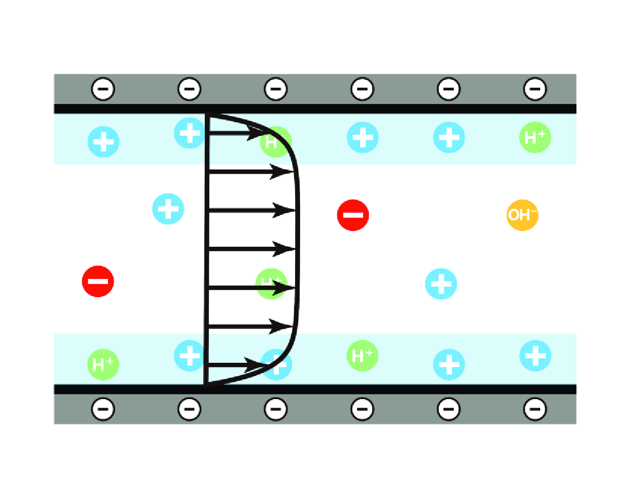
Figure 1. (a) Schematic of EOF triggered by an external electric field
 $E$
applied along a negatively charged nanochannel, where
$E$
applied along a negatively charged nanochannel, where
 $\ell$
and
$\ell$
and
 $\lambda$
are the channel size and Debye length, respectively. (b) Zoomed-in view of the ionization equilibrium of the acidic groups HA at the channel walls.
$\lambda$
are the channel size and Debye length, respectively. (b) Zoomed-in view of the ionization equilibrium of the acidic groups HA at the channel walls.
We consider a two-dimensional channel of size
 $2\ell$
(see figure 1
a), where the channel walls are negatively charged due to the ionization of acidic groups,
$2\ell$
(see figure 1
a), where the channel walls are negatively charged due to the ionization of acidic groups,
 ${\textrm{H}\textrm{A} \rightleftharpoons \textrm{A}^{-} + \textrm{H}^{+}}$
(figure 1
b). Accordingly, the surface charge density
${\textrm{H}\textrm{A} \rightleftharpoons \textrm{A}^{-} + \textrm{H}^{+}}$
(figure 1
b). Accordingly, the surface charge density
 $\sigma$
is regulated by the hydrogen ion concentration at the surface, namely the surface
$\sigma$
is regulated by the hydrogen ion concentration at the surface, namely the surface
 $\mathrm{pH}$
value. The distributions of the electrostatic potential
$\mathrm{pH}$
value. The distributions of the electrostatic potential
 $\psi$
and the ion concentrations
$\psi$
and the ion concentrations
 $n_i$
of various species
$n_i$
of various species
 $i=\pm ,{\rm H}^{+},{\rm OH}^{-}$
within the channel
$i=\pm ,{\rm H}^{+},{\rm OH}^{-}$
within the channel
 $-\ell \leq y \leq \ell$
can be obtained by solving the Poisson–Boltzmann (PB) equation:
$-\ell \leq y \leq \ell$
can be obtained by solving the Poisson–Boltzmann (PB) equation:
 \begin{align} \frac {\mathrm {d}^2\psi }{\mathrm {d} y^2}&=-\frac {e}{\epsilon _0\epsilon _r}\sum _{i} z_i n_i , \end{align}
 \begin{align} n_i &= n_{i,\infty } \exp \!\left ({-}z_i\frac {e\psi }{k_B T} \right ), \\[6pt] \nonumber \end{align}
with the boundary condition
 ${\mathrm {d} \psi }/{\mathrm {d} y} |_{y=\pm \ell }=\pm {\sigma }/ ({\epsilon _0\epsilon _r})$
. Here,
${\mathrm {d} \psi }/{\mathrm {d} y} |_{y=\pm \ell }=\pm {\sigma }/ ({\epsilon _0\epsilon _r})$
. Here,
 $e$
is the elementary charge,
$e$
is the elementary charge,
 $k_B$
is the Boltzmann constant,
$k_B$
is the Boltzmann constant,
 $T$
is the thermal temperature,
$T$
is the thermal temperature,
 $\epsilon _0$
is the vacuum permittivity,
$\epsilon _0$
is the vacuum permittivity,
 $\epsilon _r$
is the relative permittivity of water,
$\epsilon _r$
is the relative permittivity of water,
 $z_i=\pm 1$
is the valence of the ion species, and
$z_i=\pm 1$
is the valence of the ion species, and
 $n_{i,\infty }$
is the bulk ion concentration. For an acidic solution (
$n_{i,\infty }$
is the bulk ion concentration. For an acidic solution (
 $\mathrm{pH}\le 7$
), such as one prepared by adding HCl to a NaCl solution, the bulk ion concentrations are given by
$\mathrm{pH}\le 7$
), such as one prepared by adding HCl to a NaCl solution, the bulk ion concentrations are given by
 $n_{+,\infty }=n_s$
,
$n_{+,\infty }=n_s$
,
 $n_{-,\infty }=n_s+n_{{{\rm H}{+}},\infty }-n_{{{\rm OH}{-}},\infty }$
,
$n_{-,\infty }=n_s+n_{{{\rm H}{+}},\infty }-n_{{{\rm OH}{-}},\infty }$
,
 $n_{{{\rm H}{+}},\infty }=10^3N_A 10^{-\mathrm{pH}}$
and
$n_{{{\rm H}{+}},\infty }=10^3N_A 10^{-\mathrm{pH}}$
and
 $n_{{{\rm OH}{-}},\infty }=10^3 N_A 10^{-14+\mathrm{pH}}$
, where
$n_{{{\rm OH}{-}},\infty }=10^3 N_A 10^{-14+\mathrm{pH}}$
, where
 $N_A = 6.022\times 10^{23}$
is the Avogadro constant. Thus, the degree of ionization
$N_A = 6.022\times 10^{23}$
is the Avogadro constant. Thus, the degree of ionization
 $\sigma /\sigma _0$
of the charged surfaces is related to the undetermined surface electrostatic potential
$\sigma /\sigma _0$
of the charged surfaces is related to the undetermined surface electrostatic potential
 $\psi _S = \psi |_{y=\pm \ell }$
:
$\psi _S = \psi |_{y=\pm \ell }$
:
 \begin{equation} \frac {\sigma }{\sigma _0}= \frac {1}{1+10^{\textrm{p}K_a - \mathrm{pH}} \exp (-\frac {e\psi _S}{k_B T})}, \end{equation}
where
 $\sigma _0$
is the maximum surface charge density and
$\sigma _0$
is the maximum surface charge density and
 $\textrm{p}K_a$
is the ionization constant of the acidic groups (Duan et al. Reference Duan, Zhang, Chen and Chen2024).
$\textrm{p}K_a$
is the ionization constant of the acidic groups (Duan et al. Reference Duan, Zhang, Chen and Chen2024).
When an external electric field
 $E$
is applied along the channel, the Coulomb force acting on the mobile ions triggers EOF. The EOF velocity
$E$
is applied along the channel, the Coulomb force acting on the mobile ions triggers EOF. The EOF velocity
 $u$
can be determined using the Stokes equation
$u$
can be determined using the Stokes equation
 \begin{equation} \eta \frac {\mathrm {d} ^2 u}{\mathrm {d} y^2}+Ee \sum _{i} z_i n_i=0, \end{equation}
with a no-slip boundary condition
 $\left .{u}\right |_{y= \pm \ell }=0$
, where
$\left .{u}\right |_{y= \pm \ell }=0$
, where
 $\eta$
is the dynamic viscosity of the electrolyte solution (Burgreen & Nakache Reference Burgreen and Nakache1964). Accordingly, the electro-osmotic mobility
$\eta$
is the dynamic viscosity of the electrolyte solution (Burgreen & Nakache Reference Burgreen and Nakache1964). Accordingly, the electro-osmotic mobility
 $\mu _{\mathrm {eo}}$
is defined as
$\mu _{\mathrm {eo}}$
is defined as
 \begin{equation} \mu _{\mathrm {eo}}=\frac {1}{2\ell E}\int ^{\ell }_{-\ell } u\, \mathrm {d} y. \end{equation}
Now, using (2.1)–(2.4), we can theoretically predict the distributions of the electrostatic potential
 $\psi$
, ion concentration
$\psi$
, ion concentration
 $n_i$
, EOF velocity
$n_i$
, EOF velocity
 $u$
and electro-osmotic mobility
$u$
and electro-osmotic mobility
 $\mu _{\mathrm {eo}}$
in both micro- and nanochannels, and make comparisons with experiments.
$\mu _{\mathrm {eo}}$
in both micro- and nanochannels, and make comparisons with experiments.
3. Asymptotic analysis
3.1. Puzzling experimental observations
The aforementioned puzzling observations are illustrated in figure 2(a), where markers depict the experimental measurements of the electro-osmotic mobility
 $\mu _{\mathrm {eo}}$
in borosilicate glass channels at various NaCl concentrations
$\mu _{\mathrm {eo}}$
in borosilicate glass channels at various NaCl concentrations
 $n_s$
where
$n_s$
where
 $\mathrm{pH}\approx 5.5$
(Haywood et al. Reference Haywood, Harms and Jacobson2014). In the microchannel with a half-channel size of
$\mathrm{pH}\approx 5.5$
(Haywood et al. Reference Haywood, Harms and Jacobson2014). In the microchannel with a half-channel size of
 $\ell =2500\,\mathrm {nm}$
, the data represented by the blue markers show that
$\ell =2500\,\mathrm {nm}$
, the data represented by the blue markers show that
 $\mu _{\mathrm {eo}}$
decreases monotonically as
$\mu _{\mathrm {eo}}$
decreases monotonically as
 $n_s$
increases. In contrast, nanochannels with
$n_s$
increases. In contrast, nanochannels with
 $\ell =108\,$
,
$\ell =108\,$
,
 $54\,$
and
$54\,$
and
 $27\,\mathrm {nm}$
exhibit non-monotonic behaviour, where
$27\,\mathrm {nm}$
exhibit non-monotonic behaviour, where
 $\mu _{\mathrm {eo}}$
initially increases and then decreases with increasing
$\mu _{\mathrm {eo}}$
initially increases and then decreases with increasing
 $n_s$
, as indicated by the green, yellow and red markers, respectively.
$n_s$
, as indicated by the green, yellow and red markers, respectively.
To further understand this phenomenon, we look into the corresponding surface electrostatic potential
 $|\psi _S|$
measured for
$|\psi _S|$
measured for
 $\ell =2500\,\mathrm {nm}$
at various
$\ell =2500\,\mathrm {nm}$
at various
 $n_s$
, as depicted by the blue markers in figure 2(b) (Haywood et al. Reference Haywood, Harms and Jacobson2014). The results indicate that
$n_s$
, as depicted by the blue markers in figure 2(b) (Haywood et al. Reference Haywood, Harms and Jacobson2014). The results indicate that
 $|\psi _S|$
decreases with increasing
$|\psi _S|$
decreases with increasing
 $n_s$
, with data points for
$n_s$
, with data points for
 $n_s\lt 10^{-1}\,\mathrm {M}$
exceeding the DH limit, i.e.
$n_s\lt 10^{-1}\,\mathrm {M}$
exceeding the DH limit, i.e.
 $|\psi _S|\gt k_BT/e$
. Here, we have
$|\psi _S|\gt k_BT/e$
. Here, we have
 $k_BT/e \approx 25\,\mathrm {mV}$
, considering
$k_BT/e \approx 25\,\mathrm {mV}$
, considering
 $k_B=1.3804\times 10^{-23}\,\mathrm {J\,K^{-1}}$
,
$k_B=1.3804\times 10^{-23}\,\mathrm {J\,K^{-1}}$
,
 $T=300\,\mathrm {K}$
and
$T=300\,\mathrm {K}$
and
 $e=1.6\times 10^{-19}\,\mathrm {C}$
. Apparently, previous theoretical predictions derived within the DH limit are not applicable (Liu et al. Reference Liu, Tseng and Hsu2015; Sadeghi et al. Reference Sadeghi, Saidi and Sadeghi2017). Furthermore, we note that the Gouy–Chapman length
$e=1.6\times 10^{-19}\,\mathrm {C}$
. Apparently, previous theoretical predictions derived within the DH limit are not applicable (Liu et al. Reference Liu, Tseng and Hsu2015; Sadeghi et al. Reference Sadeghi, Saidi and Sadeghi2017). Furthermore, we note that the Gouy–Chapman length
 $\ell _{GC}= 2\epsilon _0 \epsilon _r k_B T/(e |\sigma |)$
, which is less than
$\ell _{GC}= 2\epsilon _0 \epsilon _r k_B T/(e |\sigma |)$
, which is less than
 $18\,\mathrm {nm}$
considering
$18\,\mathrm {nm}$
considering
 $|\sigma |\gt 0.002\,\mathrm {C\,m^{-2}}$
for typical glass surfaces in contact with aqueous solutions, is significantly smaller than the half-channel size
$|\sigma |\gt 0.002\,\mathrm {C\,m^{-2}}$
for typical glass surfaces in contact with aqueous solutions, is significantly smaller than the half-channel size
 $\ell$
. Consequently, we can derive analytical approximations for
$\ell$
. Consequently, we can derive analytical approximations for
 $\psi _S$
and
$\psi _S$
and
 $\mu _{\mathrm {eo}}$
under the conditions of
$\mu _{\mathrm {eo}}$
under the conditions of
 $|\psi _S|\gg k_B T/e$
and
$|\psi _S|\gg k_B T/e$
and
 $\ell _{GC}\ll \ell$
.
$\ell _{GC}\ll \ell$
.
3.2. Analytical predictions for the electrostatic potential

Figure 2. (a) Electro-osmotic mobility
 $\mu _{\mathrm {eo}}$
and (b) surface electrostatic potential
$\mu _{\mathrm {eo}}$
and (b) surface electrostatic potential
 $|\psi _S|$
as functions of
$|\psi _S|$
as functions of
 $n_s$
. The triangle markers represent the experimental data measured in borosilicate glass micro/nanochannels where
$n_s$
. The triangle markers represent the experimental data measured in borosilicate glass micro/nanochannels where
 $\mathrm{pH}\approx 5.5$
(Haywood et al. Reference Haywood, Harms and Jacobson2014). The coloured lines are the numerical predictions using
$\mathrm{pH}\approx 5.5$
(Haywood et al. Reference Haywood, Harms and Jacobson2014). The coloured lines are the numerical predictions using
 $\epsilon _0=8.8\times 10^{-12}\,\mathrm F\,\rm m^-{^1}$
,
$\epsilon _0=8.8\times 10^{-12}\,\mathrm F\,\rm m^-{^1}$
,
 $\epsilon _r=80$
,
$\epsilon _r=80$
,
 $k_B=1.3804\times 10^{-23}\,\mathrm J\,\rm K^-{^1}$
,
$k_B=1.3804\times 10^{-23}\,\mathrm J\,\rm K^-{^1}$
,
 $T=300\,\mathrm {K}$
,
$T=300\,\mathrm {K}$
,
 $\mathrm{pH}=5.5$
,
$\mathrm{pH}=5.5$
,
 $\textrm{p}K_a=6.6$
and
$\textrm{p}K_a=6.6$
and
 $\sigma _0=-0.45\,\mathrm C\,\rm m^-{^2}$
. The coloured arrows mark the positions where
$\sigma _0=-0.45\,\mathrm C\,\rm m^-{^2}$
. The coloured arrows mark the positions where
 $\lambda =\ell /(2\pi )$
for the corresponding curves.
$\lambda =\ell /(2\pi )$
for the corresponding curves.
The analytical predictions for the distributions of the electrostatic potential can be obtained using (2.1) and (2.2). The dimensionless forms of (2.1) and (2.2) and the corresponding boundary conditions are
 \begin{align} \frac {\mathrm {d}^2 {\Psi} }{\mathrm {d} \bar {y}^2} &= \frac {\sinh {\Psi}}{\bar {\lambda }^2},\,\,\,\,\mathrm {boundary\ conditions}\,\left .\frac {\mathrm {d} {\Psi} }{{\rm d}\bar{y}} \right |_{\bar {y}=\pm 1}=\pm \frac {\bar {\sigma }}{\bar {\lambda }^2 }, \end{align}
 \begin{align} \frac {\sigma }{\sigma _0} & = \frac {1}{1+10^{{\textrm p}K_a-\mathrm{pH}}\exp \left (-{\Psi} _S\right )}, \\[6pt] \nonumber \end{align}
where the dimensionless parameters are
 ${\Psi} =e\psi /(k_B T)$
,
${\Psi} =e\psi /(k_B T)$
,
 ${\Psi} _S=e\psi _S/(k_B T)$
,
${\Psi} _S=e\psi _S/(k_B T)$
,
 $\bar{y}=y/\ell$
,
$\bar{y}=y/\ell$
,
 $\bar {\sigma }=\sigma /(\sum _i n_{i,\infty }e \ell )$
and
$\bar {\sigma }=\sigma /(\sum _i n_{i,\infty }e \ell )$
and
 $\bar {\lambda }=\lambda /\ell$
, with
$\bar {\lambda }=\lambda /\ell$
, with
 $\lambda =\sqrt {\epsilon _0 \epsilon _r k_BT / (e^2 \sum _i{n_{i,\infty }} ) }$
being the Debye length which characterizes the thickness of the electric double layer (EDL).
$\lambda =\sqrt {\epsilon _0 \epsilon _r k_BT / (e^2 \sum _i{n_{i,\infty }} ) }$
being the Debye length which characterizes the thickness of the electric double layer (EDL).
Considering
 $|{\Psi} _S|\gg 1$
and
$|{\Psi} _S|\gg 1$
and
 $|\bar {\sigma }|/(2\bar {\lambda }^2)\gg 1$
, or equivalently
$|\bar {\sigma }|/(2\bar {\lambda }^2)\gg 1$
, or equivalently
 $|\psi _S|\gg k_B T/e$
and
$|\psi _S|\gg k_B T/e$
and
 $\ell _{GC}\ll \ell$
, the analytical approximation for the degree of ionization is derived as
$\ell _{GC}\ll \ell$
, the analytical approximation for the degree of ionization is derived as
 \begin{equation} \begin{aligned} \frac {\sigma }{\sigma _0} \approx \left (\frac {\bar {\lambda }^2}{10^{\textrm{p}K_a-\mathrm{pH}}\bar {\sigma }_0^2}\right )^{\frac {1}{3}}, \end{aligned} \end{equation}
where
 $\bar {\sigma }_0=\sigma _0/(\sum _i n_{i,\infty }e \ell )$
.
$\bar {\sigma }_0=\sigma _0/(\sum _i n_{i,\infty }e \ell )$
.
Accordingly, the electrostatic potential distributions are
 \begin{align} {\Psi} \left (\bar {y}\right )\approx\; & 4\tanh ^{-1}\left [\frac {1+\bar {\sigma }/\bar {\lambda }}{1-\bar {\sigma }/\bar {\lambda }}\exp \left(\frac {-\bar {y}-1}{\bar {\lambda }}\right)\right ]\nonumber \\ &+4\tanh ^{-1}\left [\frac {1+\bar {\sigma }/\bar {\lambda }}{1-\bar {\sigma }/\bar {\lambda }}\exp \left(\frac {\bar {y}-1}{\bar {\lambda }}\right)\right ]\,&\mathrm {for}\quad\left |{\Psi} _C\right |\ll 1. \end{align}
 \begin{align} {\Psi} \left (\bar {y}\right )\approx & -\ln \left( \frac {\pi ^2\bar {\lambda }^2}{\left (1-2\bar {\lambda }^2/\bar {\sigma }\right )^2} \left [1+\tan ^2\left (\frac {\pi \bar {y}}{2-4\bar {\lambda }^2/\bar {\sigma }}\right )\right ]\right) &\mathrm {for}\quad \left |{\Psi} _C\right |\gg 1, \\[6pt] \nonumber \end{align}
where
 ${\Psi} _C=e\psi _C/(k_B T)$
and
${\Psi} _C=e\psi _C/(k_B T)$
and
 $\psi_C=\psi|_{y=0}$
. The detailed derivations for (3.3), (3.4a
) and (3.4b
) are provided in Appendix A.
$\psi_C=\psi|_{y=0}$
. The detailed derivations for (3.3), (3.4a
) and (3.4b
) are provided in Appendix A.
Both (3.4a ) and (3.4b ) lead to the same analytical prediction of the surface electrostatic potential,
 \begin{equation} {\Psi}_S\approx -\ln \left(\frac {\bar {\sigma }^2}{\bar {\lambda }^2}\right), \end{equation}
which is the same as (A3) and (A8) in Appendix A. Considering
 $n_s\gg n_{{{\rm H}{+}},\infty }$
, (3.5) can be simplified to
$n_s\gg n_{{{\rm H}{+}},\infty }$
, (3.5) can be simplified to
 \begin{equation} \left |\frac {e\psi _S}{k_B T}\right |\approx \frac {2}{3}\ln \left [ \frac {\left |\sigma _0 \right |}{e10^{pK_a-\mathrm{pH}}}\left (\frac {n_s}{2\pi \ell _B }\right ) ^{-\frac {1}{2}}\right ], \end{equation}
where
 $\ell _B=e^2/(4\pi \epsilon _0 \epsilon _r k_B T)$
is the Bjerrum length.
$\ell _B=e^2/(4\pi \epsilon _0 \epsilon _r k_B T)$
is the Bjerrum length.
3.3. Analytical predictions for EOF
The analytical predictions for the distributions of EOF velocity can be obtained using (2.3). The dimensionless forms of (2.3) and the corresponding boundary conditions are
 \begin{equation} \frac {\mathrm {d}^2 \bar {u}}{\mathrm {d} \bar {y}^2} = \frac {\sinh {\Psi}}{\bar {\lambda }^2},\,\,\,\,\mathrm {boundary\ conditions}\,\left .\frac {\mathrm {d} \bar {u}}{{\rm d}\bar {y}} \right |_{\bar {y}=\pm 1}=0 , \end{equation}
where
 $\bar {u}=u/u_0$
and
$\bar {u}=u/u_0$
and
 $u_0=E\epsilon _0\epsilon _rk_B T/(e\eta )$
.
$u_0=E\epsilon _0\epsilon _rk_B T/(e\eta )$
.
Combining (3.1) and (3.7) yields
 \begin{equation} \bar {u}\left (\bar {y}\right )={\Psi} - {\Psi}_S. \end{equation}
Substituting (3.4a ) and (3.5) into (3.8) yields
 \begin{align} \bar {u}\left (\bar {y}\right )\approx\; & 4\tanh ^{-1}\left [\frac {1+\bar {\sigma }/\bar {\lambda }}{1-\bar {\sigma }/\bar {\lambda }}\exp \left(\frac {-\bar {y}-1}{\bar {\lambda }}\right)\right ]\nonumber \\ &+4\tanh ^{-1}\left [\frac {1+\bar {\sigma }/\bar {\lambda }}{1-\bar {\sigma }/\bar {\lambda }}\exp \left(\frac {\bar {y}-1}{\bar {\lambda }}\right)\right ]+\ln \left(\frac {\bar {\sigma }^2}{\bar {\lambda }^2}\right)\,&\mathrm {for}\quad \left |{\Psi} _C\right |\ll 1, \end{align}
 \begin{align} \bar {u}\left (\bar {y}\right )\approx & \ln \left [\frac { 1+\tan ^2\left (\frac {\pi }{2-4\bar {\lambda }^2/\bar {\sigma }}\right )}{1+\tan ^2\left (\frac {\pi \bar {y}}{2-4\bar {\lambda }^2/\bar {\sigma }}\right )}\right ]\,&\mathrm {for}\quad \left |{\Psi} _C\right |\gg 1. \\[6pt] \nonumber \end{align}
Finally, substituting (3.9a
) and (3.9b
) into (2.4), the analytical predictions for the electro-osmotic mobility
 $\mu _{\mathrm {eo}}$
are obtained:
$\mu _{\mathrm {eo}}$
are obtained:
 \begin{align} & \frac {\mu _{\mathrm {eo}}}{\mu _0}\approx \frac {2}{3}\ln \left(\frac {\left |\bar {\sigma }_0\right |}{10^{\textrm{p}K_a-\mathrm{pH}}\bar {\lambda }}\right)\quad \mathrm {for}\quad \left |{\Psi} _C\right |\ll 1, \end{align}
 \begin{align} & \frac {\mu _{\mathrm {eo}}}{\mu _0}\approx 2\ln \left [\frac {1}{2\pi \bar {\lambda }}\left (\frac {\left |\bar {\sigma }_0\right |}{10^{\textrm{p}K_a-\mathrm{pH}}\bar {\lambda }}\right )^{\frac {1}{3}}+1\right ]\quad \mathrm {for}\quad \left |{\Psi} _C\right |\gg 1, \\[6pt] \nonumber \end{align}
where
 $\mu _0=\epsilon _0\epsilon _rk_B T/(e\eta )$
is introduced for normalization. The threshold
$\mu _0=\epsilon _0\epsilon _rk_B T/(e\eta )$
is introduced for normalization. The threshold
 $|{\Psi} _C|\approx 1$
is equivalent to
$|{\Psi} _C|\approx 1$
is equivalent to
 \begin{equation} \lambda \approx \frac {\ell }{2\pi }, \end{equation}
which is obtained analytically by determining the intersection point of (3.10a
) and (3.10b
). Considering
 $n_s\gg n_{{{\rm H}{+}},\infty }$
, (3.10a
) and (3.10b
) can be simplified to
$n_s\gg n_{{{\rm H}{+}},\infty }$
, (3.10a
) and (3.10b
) can be simplified to
 \begin{align} \frac {\mu _{\mathrm {eo}}}{\mu _0}\approx \frac {2}{3}\ln \left [ \frac {\left |\sigma _0 \right |}{e10^{\textrm{p}K_a-\mathrm{pH}}}\left (\frac {n_s}{2\pi \ell _B }\right ) ^{-\frac {1}{2}}\right ]\quad \mathrm {for}\quad \lambda \ll \frac {\ell }{2\pi }, \end{align}
 \begin{align} \frac {\mu _{\mathrm {eo}}}{\mu _0}\approx 2 \ln \left [\left ( \frac {4\ell _B^2 \left |\sigma _0\right | n_s \ell ^3}{\pi e 10^{\textrm{p}K_a-\mathrm{pH}} } \right )^{\frac {1}{3}} +1\right ] \quad \mathrm {for}\quad \lambda \gg \frac {\ell }{2\pi }. \\[6pt] \nonumber \end{align}
Here, combining (3.6) and (3.12a
), we obtain
 $\mu _{\mathrm {eo}}/\mu _0 = e | \psi _S |/ (k_BT )$
, which aligns with the Helmholtz–Smoluchowski (HS) theory. In contrast, when the Debye length becomes larger than the channel size, i.e.
$\mu _{\mathrm {eo}}/\mu _0 = e | \psi _S |/ (k_BT )$
, which aligns with the Helmholtz–Smoluchowski (HS) theory. In contrast, when the Debye length becomes larger than the channel size, i.e.
 $\lambda \gg \ell /(2\pi )$
, the ratio
$\lambda \gg \ell /(2\pi )$
, the ratio
 $\mu _{\mathrm {eo}}/\mu _0$
becomes a function of
$\mu _{\mathrm {eo}}/\mu _0$
becomes a function of
 $\ell$
, as indicated in (3.12b
).
$\ell$
, as indicated in (3.12b
).
3.4. Fitting parameters
It is important to note that two key parameters, the maximum surface charge density
 $\sigma _0$
and the ionization constant
$\sigma _0$
and the ionization constant
 $pK_a$
of the charged surfaces, are not provided in the referenced article (Haywood et al. Reference Haywood, Harms and Jacobson2014). To determine these parameters, we first fit the experimental data for
$pK_a$
of the charged surfaces, are not provided in the referenced article (Haywood et al. Reference Haywood, Harms and Jacobson2014). To determine these parameters, we first fit the experimental data for
 $|\psi _S|$
shown in figure 2(b) using (3.6). The fitting process yields
$|\psi _S|$
shown in figure 2(b) using (3.6). The fitting process yields
 $\sigma _0=-0.45\,\mathrm {C\,m^{-2}}$
and
$\sigma _0=-0.45\,\mathrm {C\,m^{-2}}$
and
 $\textrm{p}K_a=6.6$
, which are consistent with ranges reported in previous studies on glass–water interfaces (Sjöberg Reference Sjöberg1996; Mueller et al. Reference Mueller, Kammler, Wegner and Pratsinis2003). Using these fitted values, we compute the numerical predictions of
$\textrm{p}K_a=6.6$
, which are consistent with ranges reported in previous studies on glass–water interfaces (Sjöberg Reference Sjöberg1996; Mueller et al. Reference Mueller, Kammler, Wegner and Pratsinis2003). Using these fitted values, we compute the numerical predictions of
 $|\psi _S|$
for various values of
$|\psi _S|$
for various values of
 $\ell$
, as shown by the coloured lines in figure 2(b), which exhibit close alignment. We then calculate the corresponding numerical predictions of
$\ell$
, as shown by the coloured lines in figure 2(b), which exhibit close alignment. We then calculate the corresponding numerical predictions of
 $\mu _{\mathrm {eo}}$
for various values of
$\mu _{\mathrm {eo}}$
for various values of
 $\ell$
, as represented by the coloured lines in figure 2(a). These predictions fit well with both the experimental data and the theoretical predictions from (3.12a
) and (3.12b
) in the corresponding regimes. Notably, the results indicate that the HS theory is applicable only in microchannels or at high salt concentrations, provided the condition
$\ell$
, as represented by the coloured lines in figure 2(a). These predictions fit well with both the experimental data and the theoretical predictions from (3.12a
) and (3.12b
) in the corresponding regimes. Notably, the results indicate that the HS theory is applicable only in microchannels or at high salt concentrations, provided the condition
 $\lambda \ll \ell /(2\pi )$
is satisfied.
$\lambda \ll \ell /(2\pi )$
is satisfied.
4. Discussion
4.1. Influence of channel size

Figure 3. (a) Numerical predictions for the spatial distributions of dimensionless electrostatic potential
 $e|\psi |/(k_B T)$
with various
$e|\psi |/(k_B T)$
with various
 $\ell$
considering
$\ell$
considering
 $n_s=10^{-4}\,\mathrm {M}$
(or equivalently
$n_s=10^{-4}\,\mathrm {M}$
(or equivalently
 $\lambda =30.2\,\mathrm {nm}$
), where the dashed and dotted lines are the corresponding analytical predictions using (3.4a
) and (3.4b
), respectively. (b) Numerical predictions for the dimensionless EOF velocity
$\lambda =30.2\,\mathrm {nm}$
), where the dashed and dotted lines are the corresponding analytical predictions using (3.4a
) and (3.4b
), respectively. (b) Numerical predictions for the dimensionless EOF velocity
 $u/u_0$
with various
$u/u_0$
with various
 $\ell$
considering
$\ell$
considering
 $n_s=10^{-4}\,\mathrm {M}$
(or equivalently
$n_s=10^{-4}\,\mathrm {M}$
(or equivalently
 $\lambda =30.2\,\mathrm {nm}$
), where the dashed and dotted lines are the corresponding analytical predictions using (3.9a
) and (3.9b
), respectively. Other parameters are identical to those used in figure 2.
$\lambda =30.2\,\mathrm {nm}$
), where the dashed and dotted lines are the corresponding analytical predictions using (3.9a
) and (3.9b
), respectively. Other parameters are identical to those used in figure 2.
To clarify the effect of channel size on EOF, we present the predicted distributions of the dimensionless electrostatic potential
 $e|\psi |/(k_B T)$
and EOF velocity
$e|\psi |/(k_B T)$
and EOF velocity
 $u/u_0$
within the channel at
$u/u_0$
within the channel at
 $n_s=10^{-4}\,\mathrm {M}$
for various
$n_s=10^{-4}\,\mathrm {M}$
for various
 $\ell$
in figure 3(a,b), respectively. The Debye length
$\ell$
in figure 3(a,b), respectively. The Debye length
 $\lambda$
is approximately
$\lambda$
is approximately
 $30 \,\mathrm {nm}$
, remaining constant for
$30 \,\mathrm {nm}$
, remaining constant for
 $n_s=10^{-4}\,\mathrm {M}$
and
$n_s=10^{-4}\,\mathrm {M}$
and
 $\mathrm{pH}=5.5$
. Figure 3(a) shows that while the centre electrostatic potential
$\mathrm{pH}=5.5$
. Figure 3(a) shows that while the centre electrostatic potential
 $|\psi _C|$
increases as
$|\psi _C|$
increases as
 $\ell$
decreases, the surface electrostatic potential
$\ell$
decreases, the surface electrostatic potential
 $|\psi _S|$
remains independent of
$|\psi _S|$
remains independent of
 $\ell$
. This behaviour arises because the analysed cases fall within the regime where
$\ell$
. This behaviour arises because the analysed cases fall within the regime where
 $\ell _{GC}\ll \ell$
. According to (2.2), the surface charge density
$\ell _{GC}\ll \ell$
. According to (2.2), the surface charge density
 $\sigma$
is also unaffected by
$\sigma$
is also unaffected by
 $\ell$
, ensuring that the total net charge
$\ell$
, ensuring that the total net charge
 $\int _{-\ell }^\ell {n_{{net}}} \, {\rm d}y$
remains constant due to electroneutrality, where
$\int _{-\ell }^\ell {n_{{net}}} \, {\rm d}y$
remains constant due to electroneutrality, where
 $n_{{net}}=\sum _i {z_i n_i}$
represents the net charge density. As
$n_{{net}}=\sum _i {z_i n_i}$
represents the net charge density. As
 $\ell$
decreases to the order of
$\ell$
decreases to the order of
 $\lambda$
, the EDLs on both sides of the channel generally converge, leading to an increase in
$\lambda$
, the EDLs on both sides of the channel generally converge, leading to an increase in
 $|\psi _C|$
. In figure 3(b), a plug-like velocity profile is shown for the EOF velocity
$|\psi _C|$
. In figure 3(b), a plug-like velocity profile is shown for the EOF velocity
 $u/u_0$
in the microchannel with
$u/u_0$
in the microchannel with
 $\ell =2500 \,\mathrm {nm}$
. This occurs because the driving Coulomb force of the EOF is concentrated within the EDL, the length scale of which is significantly smaller than the half-channel size, i.e.
$\ell =2500 \,\mathrm {nm}$
. This occurs because the driving Coulomb force of the EOF is concentrated within the EDL, the length scale of which is significantly smaller than the half-channel size, i.e.
 $\lambda \ll \ell$
(Burgreen & Nakache Reference Burgreen and Nakache1964; Arulanandam & Li Reference Arulanandam and Li2000). The plateau value can be captured by the HS equation
$\lambda \ll \ell$
(Burgreen & Nakache Reference Burgreen and Nakache1964; Arulanandam & Li Reference Arulanandam and Li2000). The plateau value can be captured by the HS equation
 $u=u_0 e|\psi _S|/(k_B T)$
, which remains constant for even larger
$u=u_0 e|\psi _S|/(k_B T)$
, which remains constant for even larger
 $\ell$
. In contrast, as
$\ell$
. In contrast, as
 $\ell$
approaches the scale of
$\ell$
approaches the scale of
 $\lambda$
, the plug-like profile diminishes and
$\lambda$
, the plug-like profile diminishes and
 $u/u_0$
decreases due to the increasing spatial confinement.
$u/u_0$
decreases due to the increasing spatial confinement.
4.2. Influence of salt concentration

Figure 4. Numerical predictions for the spatial distributions of net charge density
 $n_{net}=n_+-n_-+n_{{{\rm H}{+}}}-n_{{{\rm OH}{-}}}$
(colourmaps) and dimensionless EOF velocity
$n_{net}=n_+-n_-+n_{{{\rm H}{+}}}-n_{{{\rm OH}{-}}}$
(colourmaps) and dimensionless EOF velocity
 $u/u_0$
(solid lines) in the nanochannel with
$u/u_0$
(solid lines) in the nanochannel with
 $\ell =27\,\mathrm {nm}$
for various
$\ell =27\,\mathrm {nm}$
for various
 $n_s$
. Numerical predictions for the degree of ionization
$n_s$
. Numerical predictions for the degree of ionization
 $\sigma /\sigma _0$
at each
$\sigma /\sigma _0$
at each
 $n_s$
are marked in the corresponding subplot. Other parameters are identical with those used in figure 2.
$n_s$
are marked in the corresponding subplot. Other parameters are identical with those used in figure 2.
To elucidate the impact of salt concentration
 $n_s$
on EOF in nanochannels, we visualize the distributions of net charge density
$n_s$
on EOF in nanochannels, we visualize the distributions of net charge density
 $n_{{net}}$
and dimensionless EOF velocity
$n_{{net}}$
and dimensionless EOF velocity
 $u/u_0$
at different
$u/u_0$
at different
 $n_s$
for
$n_s$
for
 $\ell =27\,\mathrm {nm}$
in figure 4. The degree of ionization
$\ell =27\,\mathrm {nm}$
in figure 4. The degree of ionization
 $\sigma /\sigma _0$
for each case is indicated in the corner, showing an increase with the addition of salt due to the
$\sigma /\sigma _0$
for each case is indicated in the corner, showing an increase with the addition of salt due to the
 $\mathrm{pH}$
-regulation effect. At low salt concentrations, i.e.
$\mathrm{pH}$
-regulation effect. At low salt concentrations, i.e.
 $n_s=10^{-4} \,\mathrm {M}$
and
$n_s=10^{-4} \,\mathrm {M}$
and
 $n_s= 10^{-3}\,\mathrm {M}$
as indicated in figure 4(a,b), wide diffusive layers are observed because the EDL thicknesses, i.e.
$n_s= 10^{-3}\,\mathrm {M}$
as indicated in figure 4(a,b), wide diffusive layers are observed because the EDL thicknesses, i.e.
 $\lambda \approx 30 \,\mathrm {nm}$
and
$\lambda \approx 30 \,\mathrm {nm}$
and
 $\lambda \approx 10 \,\mathrm {nm}$
, respectively, are large compared with the half-channel size. Consequently, the driving Coulomb force of the EOF is evenly distributed across the channel, leading to parabolic-like velocity profiles. Meanwhile, as the degree of ionization
$\lambda \approx 10 \,\mathrm {nm}$
, respectively, are large compared with the half-channel size. Consequently, the driving Coulomb force of the EOF is evenly distributed across the channel, leading to parabolic-like velocity profiles. Meanwhile, as the degree of ionization
 $\sigma /\sigma _0$
for
$\sigma /\sigma _0$
for
 $n_s= 10^{-3}\,\mathrm {M}$
is higher than that for
$n_s= 10^{-3}\,\mathrm {M}$
is higher than that for
 $n_s=10^{-4} \,\mathrm {M}$
, the driving Coulomb force is stronger for
$n_s=10^{-4} \,\mathrm {M}$
, the driving Coulomb force is stronger for
 $n_s= 10^{-3}\,\mathrm {M}$
, resulting in a greater EOF rate compared with
$n_s= 10^{-3}\,\mathrm {M}$
, resulting in a greater EOF rate compared with
 $n_s=10^{-4} \,\mathrm {M}$
. At high salt concentrations, i.e.
$n_s=10^{-4} \,\mathrm {M}$
. At high salt concentrations, i.e.
 $n_s=10^{-2} \,\mathrm {M}$
and
$n_s=10^{-2} \,\mathrm {M}$
and
 $n_s= 10^{-1}\,\mathrm {M}$
in figure 4(c,d), net charges predominantly accumulate near the walls, resulting in plug-like velocity profiles since the corresponding Debye lengths, i.e.
$n_s= 10^{-1}\,\mathrm {M}$
in figure 4(c,d), net charges predominantly accumulate near the walls, resulting in plug-like velocity profiles since the corresponding Debye lengths, i.e.
 $\lambda \approx 3 \,\mathrm {nm}$
and
$\lambda \approx 3 \,\mathrm {nm}$
and
 $\lambda \approx 1 \,\mathrm {nm}$
, respectively, are small compared with the half-channel size. Moreover, the EOF at
$\lambda \approx 1 \,\mathrm {nm}$
, respectively, are small compared with the half-channel size. Moreover, the EOF at
 $n_s= 10^{-1}\,\mathrm {M}$
is more severely retarded due to wall shear stress, despite the degree of ionization
$n_s= 10^{-1}\,\mathrm {M}$
is more severely retarded due to wall shear stress, despite the degree of ionization
 $\sigma /\sigma _0$
and the driving Coulomb force being greater than those at
$\sigma /\sigma _0$
and the driving Coulomb force being greater than those at
 $n_s= 10^{-2}\,\mathrm {M}$
.
$n_s= 10^{-2}\,\mathrm {M}$
.
4.3. Potential effect of the Stern layer
The Stern layer is often considered a crucial factor in charge regulation, as it is assumed that the ions are tightly adsorbed to the charged surface, leading to a linear drop in electrostatic potential. Baldessari’s model incorporates the Stern layer in its charge regulation boundary condition, expressed in our notation as
 \begin{equation} {\frac {\sigma }{\sigma _0}= \frac {1}{1+10^{\textrm{p}K_a - \mathrm{pH}} \exp \big(-\frac {e\psi _S}{k_B T}-\frac {e\sigma }{C k_B T} \big)},} \end{equation}
where
 $\sigma /C$
is the potential drop within the Stern layer and
$\sigma /C$
is the potential drop within the Stern layer and
 $C$
is the Stern layer’s phenomenological capacity (Behrens & Grier Reference Behrens and Grier2001; Baldessari Reference Baldessari2008). To evaluate the potential effects of the Stern layer, we compare the numerical predictions for
$C$
is the Stern layer’s phenomenological capacity (Behrens & Grier Reference Behrens and Grier2001; Baldessari Reference Baldessari2008). To evaluate the potential effects of the Stern layer, we compare the numerical predictions for
 $|\sigma |$
,
$|\sigma |$
,
 $|\psi _S|$
and
$|\psi _S|$
and
 $\mu _{\mathrm {eo}}$
using the two boundary conditions in (2.2) and (4.1), as shown in figure 5(a–c).
$\mu _{\mathrm {eo}}$
using the two boundary conditions in (2.2) and (4.1), as shown in figure 5(a–c).
The results indicate that the two boundary conditions yield similar predictions for smaller surface group densities of
 $\sigma _0=-0.045\,\mathrm C\,\rm m^-{^2}$
and
$\sigma _0=-0.045\,\mathrm C\,\rm m^-{^2}$
and
 $\sigma _0=-0.45\,\mathrm C\,\rm m^-{^2}$
. In contrast, for
$\sigma _0=-0.45\,\mathrm C\,\rm m^-{^2}$
. In contrast, for
 $\sigma _0=-4.5\,\mathrm C\,\rm m^-{^2}$
, the model that incorporates the Stern layer predicts slightly lower values for
$\sigma _0=-4.5\,\mathrm C\,\rm m^-{^2}$
, the model that incorporates the Stern layer predicts slightly lower values for
 $|\sigma |$
,
$|\sigma |$
,
 $|\psi _S|$
and
$|\psi _S|$
and
 $\mu _{\mathrm {eo}}$
when
$\mu _{\mathrm {eo}}$
when
 $n_s\gt 10^{-2}\,\mathrm {M}$
. Thus, we anticipate that incorporating the Stern layer is primarily necessary for surfaces with extensive chargeable groups.
$n_s\gt 10^{-2}\,\mathrm {M}$
. Thus, we anticipate that incorporating the Stern layer is primarily necessary for surfaces with extensive chargeable groups.

Figure 5. (a) Surface charge density
 $|\sigma |$
, (b) surface electrostatic potential
$|\sigma |$
, (b) surface electrostatic potential
 $|\psi _S|$
and (c) electro-osmotic mobility
$|\psi _S|$
and (c) electro-osmotic mobility
 $\mu _{\mathrm {eo}}$
as functions of
$\mu _{\mathrm {eo}}$
as functions of
 $n_s$
for different
$n_s$
for different
 $\sigma _0$
. The solid lines represent the numerical predictions obtained from the boundary condition in (2.2). The dashed lines are the numerical predictions obtained from the boundary condition in (4.1) considering
$\sigma _0$
. The solid lines represent the numerical predictions obtained from the boundary condition in (2.2). The dashed lines are the numerical predictions obtained from the boundary condition in (4.1) considering
 $C=3.0\,\mathrm {F\,m^{-2}}$
, as reported in Baldessari (Reference Baldessari2008). Other parameters are identical to those used in figure 2.
$C=3.0\,\mathrm {F\,m^{-2}}$
, as reported in Baldessari (Reference Baldessari2008). Other parameters are identical to those used in figure 2.
4.4. Range of applicability of the classical PB equation
The classical PB equation is a well-established framework for modelling electrostatic interactions. While it may be regarded as less effective at very high salt concentrations due to factors such as ion size and ion–ion correlations, it remains a valid and robust approach for the specific cases presented in our study. Please note that the salt concentrations we consider, ranging from
 $n_s=10^{-5}\,$
to
$n_s=10^{-5}\,$
to
 $1\,\mathrm {M}$
, are significantly lower than the cutoff concentration
$1\,\mathrm {M}$
, are significantly lower than the cutoff concentration
 $n_s^{cut}=a^{-3}=5 \sim 60\,\mathrm {M}$
, considering a typical ion size of
$n_s^{cut}=a^{-3}=5 \sim 60\,\mathrm {M}$
, considering a typical ion size of
 $a=0.3 {\sim} 0.7 \,\mathrm {nm}$
. This suggests that the ion size effect is negligible, thereby justifying the applicability of the classical PB equation (Storey et al. Reference Storey, Edwards, Kilic and Bazant2008). Furthermore, scenarios with salt concentrations exceeding
$a=0.3 {\sim} 0.7 \,\mathrm {nm}$
. This suggests that the ion size effect is negligible, thereby justifying the applicability of the classical PB equation (Storey et al. Reference Storey, Edwards, Kilic and Bazant2008). Furthermore, scenarios with salt concentrations exceeding
 $1\,\mathrm {M}$
are less relevant to this work, as both the EOF velocity and electro-osmotic mobility approach zero in these conditions.
$1\,\mathrm {M}$
are less relevant to this work, as both the EOF velocity and electro-osmotic mobility approach zero in these conditions.
5. Conclusion
In conclusion, when it comes to EOF at the nanoscale, the ionization of charged surfaces and the distribution of net charge across the channel emerge as more critical factors than the surface potential, as they govern both the magnitude and the spatial distribution of the Coulomb driving force of the EOF. By analysing the experimental data, fitting them with our analytical predictions, and visualizing the electrostatic potential, net charge distribution and EOF velocity profile across the channel, we provide a comprehensive explanation for the non-monotonic salt dependence of the electro-osmotic mobility in
 $\mathrm{pH}$
-regulated nanochannels. Specifically, as the salt concentration increases, the initial rise of the electro-osmotic mobility is caused by the increase of surface charge density, while the subsequent decline is induced by the increase of the wall shear stress. Furthermore, we identify a transition point at
$\mathrm{pH}$
-regulated nanochannels. Specifically, as the salt concentration increases, the initial rise of the electro-osmotic mobility is caused by the increase of surface charge density, while the subsequent decline is induced by the increase of the wall shear stress. Furthermore, we identify a transition point at
 $\lambda \approx \ell /(2\pi )$
, where the EOF velocity shifts from a parabolic-like to a plug-like profile, which has practical implications for applications such as cell manipulations at the nanoscale. Additionally, we highlight that the Helmholtz–Smoluchowski theory is applicable only to microchannels or at high salt concentrations where
$\lambda \approx \ell /(2\pi )$
, where the EOF velocity shifts from a parabolic-like to a plug-like profile, which has practical implications for applications such as cell manipulations at the nanoscale. Additionally, we highlight that the Helmholtz–Smoluchowski theory is applicable only to microchannels or at high salt concentrations where
 $\lambda \ll \ell$
, a limitation that may have been overlooked in zeta-potential measurement. We anticipate that this work will advance the understanding of EOF in nanofluidic systems, with applications ranging from particle separation and ionic valves to seawater desalination, while also providing new insights into broader electrokinetic phenomena influenced by
$\lambda \ll \ell$
, a limitation that may have been overlooked in zeta-potential measurement. We anticipate that this work will advance the understanding of EOF in nanofluidic systems, with applications ranging from particle separation and ionic valves to seawater desalination, while also providing new insights into broader electrokinetic phenomena influenced by
 $\mathrm{pH}$
regulation.
$\mathrm{pH}$
regulation.
Funding
This work was supported by the National Natural Science Foundation of China (no. 12372259).
Declaration of interests
The authors report no conflict of interest.
Data availability statement
The data that support the findings of this study are available from the corresponding author upon reasonable request.
Appendix A. Analytical approximations of the electrostatic potential and degree of ionization
We first derive the analytical approximations of
 $\Psi$
considering
$\Psi$
considering
 $|{\Psi} _S|\gg 1$
and
$|{\Psi} _S|\gg 1$
and
 $|\bar {\sigma }|/(2\bar {\lambda }^2)\gg 1$
.
$|\bar {\sigma }|/(2\bar {\lambda }^2)\gg 1$
.
When
 $|{\Psi} _C|\ll 1$
, integrating (3.1) from
$|{\Psi} _C|\ll 1$
, integrating (3.1) from
 $0$
to
$0$
to
 $\bar {y}$
, using
$\bar {y}$
, using
 $\cosh {\Psi} _C \approx 1$
and considering the symmetry at
$\cosh {\Psi} _C \approx 1$
and considering the symmetry at
 $\bar {y}=0$
, i.e.
$\bar {y}=0$
, i.e.
 $\left .\mathrm {d} {\Psi} / \mathrm {d} \bar {y}\right |_{\bar {y}=0}=0$
, we have
$\left .\mathrm {d} {\Psi} / \mathrm {d} \bar {y}\right |_{\bar {y}=0}=0$
, we have
 \begin{align} \frac {1}{2}\left (\frac {\mathrm {\rm d} {\Psi} }{\mathrm {\rm d} \bar {y}}\right )^2\approx \frac {\cosh {\Psi} -1}{\bar {\lambda }^2}, \end{align}
which yields an analytical solution,
 \begin{align} {\Psi} \left (\bar {y}\right )\approx 4\tanh ^{-1}\left [C_1\exp \left(\frac {-\bar {y}-1}{\bar {\lambda }}\right)\right ]+4\tanh ^{-1}\left [C_1\exp \left(\frac {\bar {y}-1}{\bar {\lambda }}\right)\right ], \end{align}
where the constant
 $C_1$
needs to be determined. Using the boundary condition
$C_1$
needs to be determined. Using the boundary condition
 $\left.{\mathrm {d} {\Psi} }/{{\rm d}\bar {y}} \right |_{\bar {y}=\pm 1}=\pm \ {(\bar {\sigma }}/{\bar {\lambda }^2) }$
in (A1), we obtain
$\left.{\mathrm {d} {\Psi} }/{{\rm d}\bar {y}} \right |_{\bar {y}=\pm 1}=\pm \ {(\bar {\sigma }}/{\bar {\lambda }^2) }$
in (A1), we obtain
 ${\Psi} _S\approx 2 \sinh ^{-1} ({\bar {\sigma }}/{2\bar {\lambda }} )$
. Considering
${\Psi} _S\approx 2 \sinh ^{-1} ({\bar {\sigma }}/{2\bar {\lambda }} )$
. Considering
 $|{\Psi} _S|\gg 1$
, it can be simplified to
$|{\Psi} _S|\gg 1$
, it can be simplified to
 \begin{align} {\Psi} _S\approx -\ln \left(\frac {\bar {\sigma }^2}{\bar {\lambda }^2}\right). \end{align}
Combining (A2) and (A3) gives
 $C_1\approx (1+\bar {\sigma }/\bar {\lambda })/(1-\bar {\sigma }/\bar {\lambda })$
. Substituting
$C_1\approx (1+\bar {\sigma }/\bar {\lambda })/(1-\bar {\sigma }/\bar {\lambda })$
. Substituting
 $C_1$
into (A2) yields
$C_1$
into (A2) yields
 \begin{align} {\Psi} \left (\bar {y}\right )\approx 4\tanh ^{-1}\left [\frac {1+\bar {\sigma }/\bar {\lambda }}{1-\bar {\sigma }/\bar {\lambda }}\exp \left(\frac {-\bar {y}-1}{\bar {\lambda }}\right)\right ]+4\tanh ^{-1}\left [\frac {1+\bar {\sigma }/\bar {\lambda }}{1-\bar {\sigma }/\bar {\lambda }}\exp \left(\frac {\bar {y}-1}{\bar {\lambda }}\right)\right ], \end{align}
which is the same as (3.4a ) in the main text.
When
 $|{\Psi} _C|\gg 1$
, using
$|{\Psi} _C|\gg 1$
, using
 $\sinh {\Psi} \approx \exp (-{\Psi} )/2$
, (3.1) can be simplified to
$\sinh {\Psi} \approx \exp (-{\Psi} )/2$
, (3.1) can be simplified to
 \begin{align} \frac {\mathrm {d}^2 {\Psi} }{{\rm d} \bar {y}^2} \approx -\frac {\exp (-{\Psi} )}{2\bar {\lambda }^2}, \end{align}
which yields an analytical solution,
 \begin{align} {\Psi} \left (\bar {y}\right )\approx -\ln \left(C_2\bar {\lambda }^2\left [1+\tan ^2\left (\frac {\sqrt {C_2}}{2}\bar {y}\right )\right ]\right), \end{align}
where the constant
 $C_2$
needs to be determined. Using the boundary condition
$C_2$
needs to be determined. Using the boundary condition
 $\left .\mathrm {d} {\Psi} / \mathrm {d} \bar {y}\right |_{\bar {y}=\pm 1}=\pm \bar {\sigma }/\bar {\lambda }^2$
in (A6), we have
$\left .\mathrm {d} {\Psi} / \mathrm {d} \bar {y}\right |_{\bar {y}=\pm 1}=\pm \bar {\sigma }/\bar {\lambda }^2$
in (A6), we have
 $\sqrt {C_2}/2\tan (\sqrt {C_2}/2 )\approx -\bar {\sigma }/(2\bar {\lambda }^2)$
, which leads to
$\sqrt {C_2}/2\tan (\sqrt {C_2}/2 )\approx -\bar {\sigma }/(2\bar {\lambda }^2)$
, which leads to
 $C_2\approx \pi ^2/(1-2\bar {\lambda }^2/\bar {\sigma })^2$
considering
$C_2\approx \pi ^2/(1-2\bar {\lambda }^2/\bar {\sigma })^2$
considering
 $|\bar {\sigma }|/(2\bar {\lambda }^2)\gg 1$
. Substituting
$|\bar {\sigma }|/(2\bar {\lambda }^2)\gg 1$
. Substituting
 $C_2$
into (A6) yields
$C_2$
into (A6) yields
 \begin{align} {\Psi} \left (\bar {y}\right )\approx & -\ln \left( \frac {\pi ^2\bar {\lambda }^2}{\left (1-2\bar {\lambda }^2/\bar {\sigma }\right )^2} \left [1+\tan ^2\left (\frac {\pi \bar {y}}{2-4\bar {\lambda }^2/\bar {\sigma }}\right )\right ]\right), \end{align}
which is the same as (3.4b ) in the main text. Equation (A7) further leads to
 \begin{align} {\Psi} _S\approx -\ln \left(\frac {\bar {\sigma }^2}{\bar {\lambda }^2}\right). \end{align}
Note that (A3) and (A8) are identical. Thus, we can combine these two scenarios and probe
 $\sigma /\sigma _0$
for
$\sigma /\sigma _0$
for
 $|\Psi _S|\gg 1$
and
$|\Psi _S|\gg 1$
and
 $|\bar {\sigma }|/(2\bar {\lambda }^2)\gg 1$
. Substituting (A3) or (A8) into (3.2) yields
$|\bar {\sigma }|/(2\bar {\lambda }^2)\gg 1$
. Substituting (A3) or (A8) into (3.2) yields
 \begin{align} \frac {\sigma }{\sigma _0} & \approx \left ({\frac {\bar {\lambda }^2}{\bar {\sigma }_0^210^{{\textrm p}K_a-\mathrm{pH}}}}\right )^{\frac {1}{3}} \left [\sqrt [3]{\frac {1}{2}\sqrt {1+\frac {4\bar {\lambda }^2}{27\bar {\sigma }_0^2 10^{\textrm{p}K_a-\mathrm{pH}}}}+\frac {1}{2}} \right. \nonumber\\ & \quad \left. -\sqrt [3]{\frac {1}{2}\sqrt {1+\frac {4\bar {\lambda }^2}{27\bar {\sigma }_0^2 10^{\textrm{p}K_a-\mathrm{pH}}}}-\frac {1}{2}}\right ]. \end{align}
Equation (A9) can be further simplified to
 \begin{align} \frac {\sigma }{\sigma _0} \approx \left (\frac {\bar {\lambda }^2}{10^{\textrm{p}K_a-\mathrm{pH}}\bar {\sigma }_0^2}\right )^{\frac {1}{3}} \quad \mathrm {for}\quad \frac {\left |\bar {\sigma }_0\right |}{\bar {\lambda }} \gg \sqrt {10^{\mathrm{pH}-\textrm{p}K_a}}, \end{align}
which is the same as (3.3) in the main text.


