


1 Introduction
It is well known that laminar to turbulent transition in boundary layers is strongly influenced by unsteady disturbances in the free stream. This is often the result of a sequence of events beginning with the excitation of spatially growing instability waves by the free-stream disturbances. This so-called receptivity problem differs from classical instability theory in that it leads to a boundary value problem rather than an eigenvalue problem for the Orr–Sommerfeld or Rayleigh equations, which only applies in a region where the mean flow is nearly parallel (refer to review article by Reshotko (Reference Reshotko1976)). However, the relevant boundary conditions cannot be imposed on the Orr–Sommerfeld or Rayleigh equations in the infinite Reynolds number limit being considered here. The free-stream disturbances can, however, produce unsteady boundary layer disturbances near the leading edge of the boundary layer which eventually become unstable further downstream.
Goldstein (Reference Goldstein1983) used a low frequency parameter matched asymptotic expansion to show that there is an overlap domain where appropriate asymptotic solutions to the forced boundary layer equations match onto the Tollmien–Schlichting wave solutions of the Orr–Sommerfeld equation, which applies further downstream. The Tollmien–Schlichting wave/free-stream disturbance coupling tends to be fairly weak for the two-dimensional incompressible flow considered by Goldstein (Reference Goldstein1983), primarily because the boundary layer disturbances undergo considerable decay before turning into growing Tollmien–Schlichting waves in the Orr–Sommerfeld region.
But the situation can be quite different in supersonic flows where various modes of instability, which have been well documented by Mack (Reference Mack1984), can occur. Our interest here is in the moderately supersonic regime (Mach number less than 4) where the so called 1st Mack instability mode, which results from a purely inviscid mechanism when the mean flow has a generalized inflection point, is the dominant instability. Smith (Reference Smith1989) showed that there are also viscous instabilities with obliqueness angles
 $\unicode[STIX]{x1D703}$
greater than the critical angle, say
$\unicode[STIX]{x1D703}$
greater than the critical angle, say
 $\unicode[STIX]{x1D703}_{c}$
, which is equal to the inverse cosine of the free-stream Mach number,
$\unicode[STIX]{x1D703}_{c}$
, which is equal to the inverse cosine of the free-stream Mach number,
 $\cos ^{-1}(M_{\infty }^{-1})$
. These instabilities exhibit the same triple-deck structure as the subsonic Tollmien–Schlichting waves in the vicinity of the lower branch. Their critical layers lie near the wall and their phase speeds are very small. They must therefore be generated by a wall layer mechanism analogous to the one identified by Goldstein (Reference Goldstein1983).
$\cos ^{-1}(M_{\infty }^{-1})$
. These instabilities exhibit the same triple-deck structure as the subsonic Tollmien–Schlichting waves in the vicinity of the lower branch. Their critical layers lie near the wall and their phase speeds are very small. They must therefore be generated by a wall layer mechanism analogous to the one identified by Goldstein (Reference Goldstein1983).
Ricco & Wu (Reference Ricco and Wu2007) extended the Goldstein (Reference Goldstein1983) analysis to compressible subsonic and supersonic flat plate boundary layer flows and showed that highly oblique vortical disturbances can generate the viscously unstable disturbances that are a limiting form of the instability identified by Smith (Reference Smith1989). The present paper considers the more general case where the free-stream vortical disturbances generate the complete Smith (Reference Smith1989) instability, which now comes into play when the frequency-scaled (i.e. scaled with the free-stream velocity/frequency) streamwise coordinate
 $x$
is of the order of
$x$
is of the order of
 $\unicode[STIX]{x1D716}^{-2}$
, where
$\unicode[STIX]{x1D716}^{-2}$
, where
 $\unicode[STIX]{x1D716}$
denotes the frequency parameter
$\unicode[STIX]{x1D716}$
denotes the frequency parameter
 ${\mathcal{F}}$
(defined explicitly below) to the one-sixth power. (Refer to figure 1, which will be discussed more fully below.) The instability waves can have arbitrary obliqueness angles at subsonic Mach numbers but our interest here is in the supersonic case, where
${\mathcal{F}}$
(defined explicitly below) to the one-sixth power. (Refer to figure 1, which will be discussed more fully below.) The instability waves can have arbitrary obliqueness angles at subsonic Mach numbers but our interest here is in the supersonic case, where
 $\unicode[STIX]{x1D703}$
must be greater than
$\unicode[STIX]{x1D703}$
must be greater than
 $\unicode[STIX]{x1D703}_{c}$
, since our computations show that the instability wave lower branch lies further upstream than the subsonic lower branch and much further upstream than the incompressible lower branch considered by Goldstein (Reference Goldstein1983). This means that the instability wave/free-stream disturbance coupling will be much greater in this case. The instability does not possess an upper branch in this case and matches onto a low frequency (short streamwise wavenumber) Rayleigh instability (that can be identified with the 1st Mack mode) when
$\unicode[STIX]{x1D703}_{c}$
, since our computations show that the instability wave lower branch lies further upstream than the subsonic lower branch and much further upstream than the incompressible lower branch considered by Goldstein (Reference Goldstein1983). This means that the instability wave/free-stream disturbance coupling will be much greater in this case. The instability does not possess an upper branch in this case and matches onto a low frequency (short streamwise wavenumber) Rayleigh instability (that can be identified with the 1st Mack mode) when
 $x$
is of the order of
$x$
is of the order of
 $\unicode[STIX]{x1D716}^{-4}$
.
$\unicode[STIX]{x1D716}^{-4}$
.

Figure 1. Structure of disturbance flow where
 $r$
is a real number in the range
$r$
is a real number in the range
 $0\leqslant r<1$
.
$0\leqslant r<1$
.
Fedorov & Khokhlov (Reference Fedorov and Khokhlov1991) and Fedorov (Reference Fedorov2003) (hereafter referred to as F/K) analysed the generation of inviscid instabilities in a supersonic flat plate boundary layer by fast and slow acoustic disturbances in the free stream. (The Fedorov & Khokhlov (Reference Fedorov and Khokhlov1991) analysis was two-dimensional and Fedorov (Reference Fedorov2003) extended it to include oblique disturbances.) The slow acoustic mode propagates downstream/upstream when the obliqueness angle
 $\unicode[STIX]{x1D703}$
of the acoustic disturbances is smaller/larger than the critical angle
$\unicode[STIX]{x1D703}$
of the acoustic disturbances is smaller/larger than the critical angle
 $\unicode[STIX]{x1D703}_{c}$
, which, as already indicated, corresponds to the minimum obliqueness angle of the Smith (Reference Smith1989) instabilities. Fedorov (Reference Fedorov2003) considered the case where the deviation
$\unicode[STIX]{x1D703}_{c}$
, which, as already indicated, corresponds to the minimum obliqueness angle of the Smith (Reference Smith1989) instabilities. Fedorov (Reference Fedorov2003) considered the case where the deviation
 $\unicode[STIX]{x0394}\unicode[STIX]{x1D703}\equiv \unicode[STIX]{x1D703}_{c}-\unicode[STIX]{x1D703}$
of the obliqueness angle from its critical value is
$\unicode[STIX]{x0394}\unicode[STIX]{x1D703}\equiv \unicode[STIX]{x1D703}_{c}-\unicode[STIX]{x1D703}$
of the obliqueness angle from its critical value is
 $\mathit{O}(1)$
and showed that downstream propagating slow acoustic modes with
$\mathit{O}(1)$
and showed that downstream propagating slow acoustic modes with
 $\unicode[STIX]{x0394}\unicode[STIX]{x1D703}>0$
generate unsteady boundary layer disturbances that match onto the inviscid 1st Mack mode instability without undergoing any significant decay. But the inviscid Mack mode only emerges when the frequency-scaled distance
$\unicode[STIX]{x0394}\unicode[STIX]{x1D703}>0$
generate unsteady boundary layer disturbances that match onto the inviscid 1st Mack mode instability without undergoing any significant decay. But the inviscid Mack mode only emerges when the frequency-scaled distance
 $x$
is
$x$
is
 $\mathit{O}(\unicode[STIX]{x1D716}^{-6})=\mathit{O}({\mathcal{F}}^{-1})$
which is much further downstream than the region where the long streamwise wavelength Rayleigh (1st Mack) mode emerges from the Smith (Reference Smith1989) triple-deck solution. The latter instability can, therefore, undergo considerable growth before reaching the downstream region where the inviscid Mack mode emerges from the F/K solution. This is important because (as will be shown below) this region is likely to lie too far downstream to be of practical interest when scaled up to actual flight conditions. It also turns out that the most rapidly growing instability in the moderately supersonic regime being considered here is the (usually highly oblique) 1st mode. (The obliqueness angle of the most rapidly growing 1st mode lies between
$\mathit{O}(\unicode[STIX]{x1D716}^{-6})=\mathit{O}({\mathcal{F}}^{-1})$
which is much further downstream than the region where the long streamwise wavelength Rayleigh (1st Mack) mode emerges from the Smith (Reference Smith1989) triple-deck solution. The latter instability can, therefore, undergo considerable growth before reaching the downstream region where the inviscid Mack mode emerges from the F/K solution. This is important because (as will be shown below) this region is likely to lie too far downstream to be of practical interest when scaled up to actual flight conditions. It also turns out that the most rapidly growing instability in the moderately supersonic regime being considered here is the (usually highly oblique) 1st mode. (The obliqueness angle of the most rapidly growing 1st mode lies between
 $50^{\circ }$
and
$50^{\circ }$
and
 $70^{\circ }$
for an insulated wall when the Mach number is between 2 and 6, Mack Reference Mack1984.)
$70^{\circ }$
for an insulated wall when the Mach number is between 2 and 6, Mack Reference Mack1984.)
The spanwise wavenumber of the slow acoustic mode increases as
 $\unicode[STIX]{x1D703}$
approaches
$\unicode[STIX]{x1D703}$
approaches
 $\unicode[STIX]{x1D703}_{c}$
and the F/K analysis, which is completely inviscid, breaks down when
$\unicode[STIX]{x1D703}_{c}$
and the F/K analysis, which is completely inviscid, breaks down when
 $\unicode[STIX]{x0394}\unicode[STIX]{x1D703}$
becomes sufficiently small (Fedorov Reference Fedorov2003). We extend their analysis to these small values of
$\unicode[STIX]{x0394}\unicode[STIX]{x1D703}$
becomes sufficiently small (Fedorov Reference Fedorov2003). We extend their analysis to these small values of
 $\unicode[STIX]{x0394}\unicode[STIX]{x1D703}$
and show that viscous effects come into play in the diffraction region where the slow boundary layer disturbance is generated when
$\unicode[STIX]{x0394}\unicode[STIX]{x1D703}$
and show that viscous effects come into play in the diffraction region where the slow boundary layer disturbance is generated when
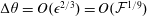 $\unicode[STIX]{x0394}\unicode[STIX]{x1D703}=\mathit{O}(\unicode[STIX]{x1D716}^{2/3})=\mathit{O}({\mathcal{F}}^{1/9})$
and that this region, as well as the downstream region where an instability wave can emerge, moves upstream as
$\unicode[STIX]{x0394}\unicode[STIX]{x1D703}=\mathit{O}(\unicode[STIX]{x1D716}^{2/3})=\mathit{O}({\mathcal{F}}^{1/9})$
and that this region, as well as the downstream region where an instability wave can emerge, moves upstream as
 $\unicode[STIX]{x0394}\unicode[STIX]{x1D703}\rightarrow 0$
. The latter region lies at an
$\unicode[STIX]{x0394}\unicode[STIX]{x1D703}\rightarrow 0$
. The latter region lies at an
 $\mathit{O}(\unicode[STIX]{x1D716}^{-(4+2r)})$
distance downstream when
$\mathit{O}(\unicode[STIX]{x1D716}^{-(4+2r)})$
distance downstream when
 $\unicode[STIX]{x0394}\unicode[STIX]{x1D703}$
is reduced to
$\unicode[STIX]{x0394}\unicode[STIX]{x1D703}$
is reduced to
 $\mathit{O}(\unicode[STIX]{x1D716}^{1-r})$
where
$\mathit{O}(\unicode[STIX]{x1D716}^{1-r})$
where
 $r$
is a real number in the range
$r$
is a real number in the range
 $1/3\leqslant r<1$
, which is downstream of the viscous triple-deck region where the Goldstein (Reference Goldstein1983)–Ricco–Wu (Reference Ricco and Wu2007) instability begins to grow (since it turns out that there are no global solutions when
$1/3\leqslant r<1$
, which is downstream of the viscous triple-deck region where the Goldstein (Reference Goldstein1983)–Ricco–Wu (Reference Ricco and Wu2007) instability begins to grow (since it turns out that there are no global solutions when
 $r<1/3$
) but can now be of considerable significance under actual flight conditions since it lies upstream of the region where the
$r<1/3$
) but can now be of considerable significance under actual flight conditions since it lies upstream of the region where the
 $\unicode[STIX]{x0394}\unicode[STIX]{x1D703}=\mathit{O}(1)$
instability begins to grow.
$\unicode[STIX]{x0394}\unicode[STIX]{x1D703}=\mathit{O}(1)$
instability begins to grow.
It is therefore reasonable to consider both the vortical and small-
 $\unicode[STIX]{x0394}\unicode[STIX]{x1D703}$
acoustic disturbances simultaneously. The vortically generated instability is likely to be more important than the acoustically generated instability since the analysis shows that the former, which comes into play when
$\unicode[STIX]{x0394}\unicode[STIX]{x1D703}$
acoustic disturbances simultaneously. The vortically generated instability is likely to be more important than the acoustically generated instability since the analysis shows that the former, which comes into play when
 $x=\mathit{O}(\unicode[STIX]{x1D716}^{-2})$
, has an
$x=\mathit{O}(\unicode[STIX]{x1D716}^{-2})$
, has an
 $\mathit{O}(\unicode[STIX]{x1D716}^{-1})$
growth rate while the maximum growth rate of the latter, which cannot come into play until
$\mathit{O}(\unicode[STIX]{x1D716}^{-1})$
growth rate while the maximum growth rate of the latter, which cannot come into play until
 $x=\mathit{O}(\unicode[STIX]{x1D716}^{-(4+2r)})$
, turns out to be
$x=\mathit{O}(\unicode[STIX]{x1D716}^{-(4+2r)})$
, turns out to be
 $\mathit{O}(1)$
.
$\mathit{O}(1)$
.
The forced slow mode generated by the F/K mechanism appears to exist for smaller obliqueness angles with
 $\unicode[STIX]{x0394}\unicode[STIX]{x1D703}<0$
, but the streamwise wavenumber then becomes negative, which means that the acoustic disturbances propagate upstream and are probably not able to directly produce 1st Mack mode instabilities which propagate downstream. The deviation angle
$\unicode[STIX]{x0394}\unicode[STIX]{x1D703}<0$
, but the streamwise wavenumber then becomes negative, which means that the acoustic disturbances propagate upstream and are probably not able to directly produce 1st Mack mode instabilities which propagate downstream. The deviation angle
 $\unicode[STIX]{x0394}\unicode[STIX]{x1D703}$
is negative for the supersonic triple-deck instabilities but the streamwise wavenumber is positive in that case and the solution can, therefore, match the downstream propagating 1st Mack mode instability.
$\unicode[STIX]{x0394}\unicode[STIX]{x1D703}$
is negative for the supersonic triple-deck instabilities but the streamwise wavenumber is positive in that case and the solution can, therefore, match the downstream propagating 1st Mack mode instability.
Fedorov (Reference Fedorov2003) showed that the F/K solution is in close agreement with the data of Maslov et al. (Reference Maslov, Shiplyuk, Sidorenko and Arnal2001) at
 $\mathit{O}(1)$
values of
$\mathit{O}(1)$
values of
 $\unicode[STIX]{x0394}\unicode[STIX]{x1D703}$
but greatly underpredicts the experimental receptivity coefficient when
$\unicode[STIX]{x0394}\unicode[STIX]{x1D703}$
but greatly underpredicts the experimental receptivity coefficient when
 $\unicode[STIX]{x0394}\unicode[STIX]{x1D703}$
is close to zero, which could be due the additional inviscid instability that evolves from the viscous triple-deck solution.
$\unicode[STIX]{x0394}\unicode[STIX]{x1D703}$
is close to zero, which could be due the additional inviscid instability that evolves from the viscous triple-deck solution.
As noted above, the present paper is concerned with the unsteady flow in a flat plate boundary layer generated by mildly oblique vortical disturbances and small-
 $\unicode[STIX]{x0394}\unicode[STIX]{x1D703}$
acoustic disturbances in a moderate supersonic Mach number free stream. It shows, among other things, that the vortical disturbances generate a viscous instability that can exhibit much less decay upstream of its lower branch than the corresponding two-dimensional subsonic modes considered by Goldstein (Reference Goldstein1983) even when the frequency parameter is small and that the resulting instabilities could, therefore, dominate over those generated by the acoustic disturbances. The relevant experiments are usually conducted with a trailing edge flap that tends to move the leading edge stagnation point to the lower surface of the plate, which could certainly cause the leading edge boundary layer to be slightly different from the Blasius boundary layer considered in the paper and thereby slightly modify the leading edge receptivity. But the present paper is meant to explain the relevant physics and we believe that this is best done by analysing the ideal situation that the experiments are meant to simulate.
$\unicode[STIX]{x0394}\unicode[STIX]{x1D703}$
acoustic disturbances in a moderate supersonic Mach number free stream. It shows, among other things, that the vortical disturbances generate a viscous instability that can exhibit much less decay upstream of its lower branch than the corresponding two-dimensional subsonic modes considered by Goldstein (Reference Goldstein1983) even when the frequency parameter is small and that the resulting instabilities could, therefore, dominate over those generated by the acoustic disturbances. The relevant experiments are usually conducted with a trailing edge flap that tends to move the leading edge stagnation point to the lower surface of the plate, which could certainly cause the leading edge boundary layer to be slightly different from the Blasius boundary layer considered in the paper and thereby slightly modify the leading edge receptivity. But the present paper is meant to explain the relevant physics and we believe that this is best done by analysing the ideal situation that the experiments are meant to simulate.
The outline of the paper is as follows. The imposed upstream disturbance environment is discussed in § 2 and the upstream boundary layer flow generated by the imposed vortical disturbances is analysed in § 3.1. Section 3.2 describes the resulting asymptotic eigensolutions produced by this flow. The slow boundary layer disturbances generated by acoustic disturbances with obliqueness angles close to the critical angle are analysed in § 4. Section 5 shows that the vortically generated asymptotic eigensolutions evolve into oblique instability waves with a viscous triple-deck structure when, as noted above, the scaled streamwise coordinate is
 $\mathit{O}(\unicode[STIX]{x1D716}^{-2})$
while the acoustically generated slow boundary disturbances do not evolve into oblique instability waves in this region and eventually develop into oblique stable disturbances with an inviscid triple-deck structure when the scaled streamwise coordinate becomes
$\mathit{O}(\unicode[STIX]{x1D716}^{-2})$
while the acoustically generated slow boundary disturbances do not evolve into oblique instability waves in this region and eventually develop into oblique stable disturbances with an inviscid triple-deck structure when the scaled streamwise coordinate becomes
 $\mathit{O}(\unicode[STIX]{x1D716}^{-(2+4r)})$
,
$\mathit{O}(\unicode[STIX]{x1D716}^{-(2+4r)})$
,
 $1/3\leqslant r<1$
. Section 6 shows that both the vortically generated instability and the acoustically generated oblique disturbance eventually evolve into modified Rayleigh-type instabilities at larger downstream distances. The numerical procedures are described in § 7. The numerical results are presented in § 8 and their physical implications are discussed. Some final conclusions are given in § 9.
$1/3\leqslant r<1$
. Section 6 shows that both the vortically generated instability and the acoustically generated oblique disturbance eventually evolve into modified Rayleigh-type instabilities at larger downstream distances. The numerical procedures are described in § 7. The numerical results are presented in § 8 and their physical implications are discussed. Some final conclusions are given in § 9.
2 Formulation
We consider a supersonic flow of an ideal gas with uniform free-stream velocity
 $U_{\infty }^{\ast }$
, temperature
$U_{\infty }^{\ast }$
, temperature
 $T_{\infty }^{\ast }$
, dynamic viscosity
$T_{\infty }^{\ast }$
, dynamic viscosity
 $\unicode[STIX]{x1D707}_{\infty }^{\ast }$
and density
$\unicode[STIX]{x1D707}_{\infty }^{\ast }$
and density
 $\unicode[STIX]{x1D70C}_{\infty }^{\ast }$
past an infinitely thin flat plate and suppose that a small amplitude harmonic distortion with angular frequency
$\unicode[STIX]{x1D70C}_{\infty }^{\ast }$
past an infinitely thin flat plate and suppose that a small amplitude harmonic distortion with angular frequency
 $\unicode[STIX]{x1D714}^{\ast }$
is superimposed on the flow. We also suppose that the time
$\unicode[STIX]{x1D714}^{\ast }$
is superimposed on the flow. We also suppose that the time
 $t$
is normalized by
$t$
is normalized by
 $\unicode[STIX]{x1D714}^{\ast }$
, the velocities by
$\unicode[STIX]{x1D714}^{\ast }$
, the velocities by
 $U_{\infty }^{\ast }$
, the pressure fluctuation by
$U_{\infty }^{\ast }$
, the pressure fluctuation by
 $\unicode[STIX]{x1D70C}_{\infty }^{\ast }(U_{\infty }^{\ast })^{2}$
, the temperature by
$\unicode[STIX]{x1D70C}_{\infty }^{\ast }(U_{\infty }^{\ast })^{2}$
, the temperature by
 $T_{\infty }^{\ast }$
and the dynamic viscosity by
$T_{\infty }^{\ast }$
and the dynamic viscosity by
 $\unicode[STIX]{x1D707}_{\infty }^{\ast }$
. We let
$\unicode[STIX]{x1D707}_{\infty }^{\ast }$
. We let
 $\{x,y,z\}$
denote Cartesian coordinates normalized by
$\{x,y,z\}$
denote Cartesian coordinates normalized by
 $L^{\ast }\equiv U_{\infty }^{\ast }/\unicode[STIX]{x1D714}^{\ast }$
with the coordinate
$L^{\ast }\equiv U_{\infty }^{\ast }/\unicode[STIX]{x1D714}^{\ast }$
with the coordinate
 $y$
being perpendicular to the surface of the plate.
$y$
being perpendicular to the surface of the plate.
As indicated in the introduction, the present paper assumes the Reynolds number
 $\unicode[STIX]{x1D70C}^{\ast }U_{\infty }^{\ast }L^{\ast }/\unicode[STIX]{x1D707}_{\infty }^{\ast }$
to be large and uses asymptotic theory to explain how the imposed harmonic distortion generates oblique instabilities at large downstream distances in the viscous boundary layer that forms on the surface of the plate. The distortion will therefore be inviscid at lowest approximation and, as is well known (Kovasznay Reference Kovasznay1953), can be decomposed into an acoustic component that carries no vorticity, and vortical and entropic components that produce no pressure fluctuations.
$\unicode[STIX]{x1D70C}^{\ast }U_{\infty }^{\ast }L^{\ast }/\unicode[STIX]{x1D707}_{\infty }^{\ast }$
to be large and uses asymptotic theory to explain how the imposed harmonic distortion generates oblique instabilities at large downstream distances in the viscous boundary layer that forms on the surface of the plate. The distortion will therefore be inviscid at lowest approximation and, as is well known (Kovasznay Reference Kovasznay1953), can be decomposed into an acoustic component that carries no vorticity, and vortical and entropic components that produce no pressure fluctuations.
We only consider the first two for simplicity. The vortical velocity
 $\boldsymbol{u}_{v}$
is given by
$\boldsymbol{u}_{v}$
is given by
 $$\begin{eqnarray}\boldsymbol{u}_{v}=\{u_{v},v_{v},w_{v}\}=\hat{\unicode[STIX]{x1D6FF}}\{u_{\infty },v_{\infty },w_{\infty }\}\exp [\text{i}(x-t+\unicode[STIX]{x1D6FE}y+\unicode[STIX]{x1D6FD}z)],\end{eqnarray}$$
where
 $\hat{\unicode[STIX]{x1D6FF}}\ll 1$
and
$\hat{\unicode[STIX]{x1D6FF}}\ll 1$
and
 $u_{\infty },v_{\infty },w_{\infty }$
satisfy the continuity condition
$u_{\infty },v_{\infty },w_{\infty }$
satisfy the continuity condition
 $$\begin{eqnarray}u_{\infty }+\unicode[STIX]{x1D6FE}v_{\infty }+\unicode[STIX]{x1D6FD}w_{\infty }=0\end{eqnarray}$$
but are otherwise arbitrary constants while the acoustic component is governed by the linear wave equation which has a fundamental plane wave solution
 $$\begin{eqnarray}\{\boldsymbol{u}_{a},p_{a}\}=\{u_{a},v_{a},w_{a},p_{a}\}=\frac{\hat{\unicode[STIX]{x1D6FF}}p_{\infty }}{1-\unicode[STIX]{x1D6FC}}\{\unicode[STIX]{x1D6FC},\unicode[STIX]{x1D6FE},\unicode[STIX]{x1D6FD},1-\unicode[STIX]{x1D6FC}\}\exp [\text{i}(\unicode[STIX]{x1D6FC}x+\unicode[STIX]{x1D6FE}y+\unicode[STIX]{x1D6FD}z-t)],\end{eqnarray}$$
for the velocity and pressure perturbation where
 $$\begin{eqnarray}\unicode[STIX]{x1D6FE}=\sqrt{(M_{\infty }^{2}-1)(\unicode[STIX]{x1D6FC}-\unicode[STIX]{x1D6FC}_{1})(\unicode[STIX]{x1D6FC}-\unicode[STIX]{x1D6FC}_{2})},\quad \unicode[STIX]{x1D6FC}_{1,2}=\frac{M_{\infty }^{2}\pm \sqrt{M_{\infty }^{2}+\unicode[STIX]{x1D6FD}^{2}(M_{\infty }^{2}-1)}}{M_{\infty }^{2}-1},\end{eqnarray}$$
where, as noted in the introduction,
 $M_{\infty }$
denotes the free-stream Mach number.
$M_{\infty }$
denotes the free-stream Mach number.
The leading edge interaction will produce large scattered fields when the incidence angle
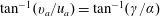 $\tan ^{-1}(v_{a}/u_{a})=\tan ^{-1}(\unicode[STIX]{x1D6FE}/\unicode[STIX]{x1D6FC})$
of the acoustic wave and
$\tan ^{-1}(v_{a}/u_{a})=\tan ^{-1}(\unicode[STIX]{x1D6FE}/\unicode[STIX]{x1D6FC})$
of the acoustic wave and
 $\tan ^{-1}(v_{v}/u_{v})$
of the vortical disturbance are
$\tan ^{-1}(v_{v}/u_{v})$
of the vortical disturbance are
 $\mathit{O}(1)$
. In order to avoid this complication, we only consider the case where the incidence angle of the vortical disturbance is small, which requires that
$\mathit{O}(1)$
. In order to avoid this complication, we only consider the case where the incidence angle of the vortical disturbance is small, which requires that
 $$\begin{eqnarray}\frac{v_{\infty }}{u_{\infty }}\ll 1\end{eqnarray}$$
and the case where the incidence angle of the acoustic disturbance is zero, which requires that
 $$\begin{eqnarray}\unicode[STIX]{x1D6FC}=\unicode[STIX]{x1D6FC}_{\mp }=\frac{M_{\infty }\cos \unicode[STIX]{x1D703}}{M_{\infty }\cos \unicode[STIX]{x1D703}\mp 1},\quad \unicode[STIX]{x1D703}\equiv \tan ^{-1}\left(\frac{\unicode[STIX]{x1D6FD}}{\unicode[STIX]{x1D6FC}}\right),\end{eqnarray}$$
where the subscripts
 $\mp$
refer to the slow/fast acoustic modes. Equation (2.6) shows that the slow mode wavenumber becomes infinite when the obliqueness angle is equal to the critical angle referred to in the introduction.
$\mp$
refer to the slow/fast acoustic modes. Equation (2.6) shows that the slow mode wavenumber becomes infinite when the obliqueness angle is equal to the critical angle referred to in the introduction.
As indicated above our interest here is in explaining how the incident harmonic distortions generate oblique instabilities at large downstream distances in the viscous boundary layer where the mean temperature, density and streamwise velocity, say
 $T$
,
$T$
,
 $\unicode[STIX]{x1D70C}$
,
$\unicode[STIX]{x1D70C}$
,
 $U$
, respectively, can be expressed as functions of the Dorodnitsyn–Howarth variable
$U$
, respectively, can be expressed as functions of the Dorodnitsyn–Howarth variable
 $$\begin{eqnarray}\unicode[STIX]{x1D702}\equiv \frac{1}{\unicode[STIX]{x1D716}^{3}\sqrt{2x}}\int _{0}^{y}\unicode[STIX]{x1D70C}(x,{\tilde{y}})\,\text{d}y\end{eqnarray}$$
and determined from the similarity equations (Stewartson Reference Stewartson1964)
 $$\begin{eqnarray}\displaystyle & U=F^{\prime }(\unicode[STIX]{x1D702}), & \displaystyle\end{eqnarray}$$
 $$\begin{eqnarray}\displaystyle & \displaystyle \left(\frac{\unicode[STIX]{x1D707}F^{\prime \prime }}{T}\right)^{\prime }+FF^{\prime \prime }=0, & \displaystyle\end{eqnarray}$$
 $$\begin{eqnarray}\displaystyle & \displaystyle \mathit{Pr}^{-1}\left(\frac{\unicode[STIX]{x1D707}T^{\prime }}{T}\right)^{\prime }+FT^{\prime }+(\unicode[STIX]{x1D6FE}_{r}-1)M_{\infty }^{2}(F^{\prime \prime })^{2}=0, & \displaystyle\end{eqnarray}$$
 $$\begin{eqnarray}\displaystyle & \unicode[STIX]{x1D70C}T=1, & \displaystyle\end{eqnarray}$$
 $$\begin{eqnarray}\displaystyle & F(0)=F^{\prime }(0)=0,T^{\prime }(0)=0;\quad F^{\prime }\rightarrow 1,T\rightarrow 1\quad \text{as }\unicode[STIX]{x1D702}\rightarrow \infty , & \displaystyle\end{eqnarray}$$
where
 $\unicode[STIX]{x1D6FE}_{r}$
is the specific heat ratio and the mean viscosity
$\unicode[STIX]{x1D6FE}_{r}$
is the specific heat ratio and the mean viscosity
 $\unicode[STIX]{x1D707}$
is assumed to depend on the temperature. The prime is used to denote differentiation with respect to
$\unicode[STIX]{x1D707}$
is assumed to depend on the temperature. The prime is used to denote differentiation with respect to
 $\unicode[STIX]{x1D702}$
and
$\unicode[STIX]{x1D702}$
and
 $\mathit{Pr}$
is used to denote the Prandtl number.
$\mathit{Pr}$
is used to denote the Prandtl number.
The natural small parameter for the asymptotic expansion turns out to be
 $$\begin{eqnarray}\unicode[STIX]{x1D716}\equiv {\mathcal{F}}^{1/6},\end{eqnarray}$$
where, as indicated in the introduction,
 $$\begin{eqnarray}{\mathcal{F}}\equiv \frac{\unicode[STIX]{x1D714}^{\ast }\unicode[STIX]{x1D707}_{\infty }^{\ast }}{\unicode[STIX]{x1D70C}_{\infty }^{\ast }(U_{\infty }^{\ast })^{2}}\end{eqnarray}$$
denotes the frequency parameter. We begin by considering the unsteady flow generated by the upstream vorticity.
3 Boundary layer disturbances generated by free-stream vorticity
3.1 Leading edge region
Our interest here is in boundary layer disturbances that generate oblique viscous instabilities in a triple-deck region that lies at an
 $\mathit{O}(\unicode[STIX]{x1D716}^{-2})$
distance downstream. These instabilities, as will be shown below, will have
$\mathit{O}(\unicode[STIX]{x1D716}^{-2})$
distance downstream. These instabilities, as will be shown below, will have
 $\mathit{O}(\unicode[STIX]{x1D716}^{-1})$
spanwise wavenumbers. And we therefore require that
$\mathit{O}(\unicode[STIX]{x1D716}^{-1})$
spanwise wavenumbers. And we therefore require that
 $$\begin{eqnarray}\overline{\unicode[STIX]{x1D6FD}}\equiv \unicode[STIX]{x1D716}\unicode[STIX]{x1D6FD}=\mathit{O}(1)\end{eqnarray}$$
since the spanwise wavenumber must remain constant as the disturbances propagate downstream. The continuity condition (2.2) will then require that
 $$\begin{eqnarray}\overline{w}_{\infty }\equiv \frac{w_{\infty }}{\unicode[STIX]{x1D716}}=\mathit{O}(1)\end{eqnarray}$$
and the obliqueness requirement (2.5) can be satisfied if we require that
 $$\begin{eqnarray}\overline{v}_{\infty }\equiv \frac{v_{\infty }}{\unicode[STIX]{x1D716}}=\mathit{O}(1).\end{eqnarray}$$
Equation (2.2) then becomes
 $$\begin{eqnarray}u_{\infty }+\overline{\unicode[STIX]{x1D6FE}}~\overline{v}_{\infty }+\overline{\unicode[STIX]{x1D6FD}}\overline{w}_{\infty }=0,\end{eqnarray}$$
where
 $$\begin{eqnarray}\overline{\unicode[STIX]{x1D6FE}}\equiv \unicode[STIX]{x1D716}\unicode[STIX]{x1D6FE}=\mathit{O}(1).\end{eqnarray}$$
The vortical velocity (2.1) will then interact with the plate to produce the following inviscid velocity field (Ricco & Wu Reference Ricco and Wu2007):
 $$\begin{eqnarray}\displaystyle \boldsymbol{u}_{v}(x,y,z) & = & \displaystyle \hat{\unicode[STIX]{x1D6FF}}\left\{u_{\infty }\text{e}^{\text{i}\overline{\unicode[STIX]{x1D6FE}}y/\unicode[STIX]{x1D716}}+\text{i}\unicode[STIX]{x1D716}^{2}\frac{\overline{v}_{\infty }}{\overline{g}}\text{e}^{-\overline{g}y/\unicode[STIX]{x1D716}},\unicode[STIX]{x1D716}\overline{v}_{\infty }(\text{e}^{\text{i}\overline{\unicode[STIX]{x1D6FE}}y/\unicode[STIX]{x1D716}}-\text{e}^{-\overline{g}y/\unicode[STIX]{x1D716}}),\right.\nonumber\\ \displaystyle & & \displaystyle \left.\unicode[STIX]{x1D716}\left(\overline{w}_{\infty }\text{e}^{\text{i}\overline{\unicode[STIX]{x1D6FE}}y/\unicode[STIX]{x1D716}}+\text{i}\overline{v}_{\infty }\frac{\overline{\unicode[STIX]{x1D6FD}}}{\overline{g}}\text{e}^{-\overline{g}y/\unicode[STIX]{x1D716}}\right)\right\}\text{e}^{\text{i}(x-t+\overline{\unicode[STIX]{x1D6FD}}z/\unicode[STIX]{x1D716})},\end{eqnarray}$$
 $$\begin{eqnarray}\overline{g}\equiv \unicode[STIX]{x1D716}\sqrt{1+\left(\frac{\overline{\unicode[STIX]{x1D6FD}}}{\unicode[STIX]{x1D716}}\right)^{2}}=\overline{\unicode[STIX]{x1D6FD}}+\frac{\unicode[STIX]{x1D716}^{2}}{2\overline{\unicode[STIX]{x1D6FD}}}+\cdots \,,\end{eqnarray}$$
when the streamwise coordinate
 $x$
is assumed to be large enough so that the leading edge refraction effects have decayed.
$x$
is assumed to be large enough so that the leading edge refraction effects have decayed.
As noted above the free-stream disturbance (2.1) generates a slip velocity at the surface of the plate that must be brought to zero in a thin viscous boundary layer whose mean velocity and temperature are given by (2.7)–(2.12). We begin by considering the flow in the vicinity of the leading edge where the streamwise length scale is
 $x=\mathit{O}(1)$
. Since (3.6) depends on the streamwise coordinate only through this relatively long streamwise length scale, the solution
$x=\mathit{O}(1)$
. Since (3.6) depends on the streamwise coordinate only through this relatively long streamwise length scale, the solution
 $\{u,v,w,\unicode[STIX]{x1D717}\}$
for the velocity and temperature in this region is given by (Ricco & Wu Reference Ricco and Wu2007)
$\{u,v,w,\unicode[STIX]{x1D717}\}$
for the velocity and temperature in this region is given by (Ricco & Wu Reference Ricco and Wu2007)
 $$\begin{eqnarray}\displaystyle \{u,v,w,\unicode[STIX]{x1D717}\} & = & \displaystyle \left\{F^{\prime }(\unicode[STIX]{x1D702}),\frac{\unicode[STIX]{x1D716}^{3}T}{\sqrt{2x}}\left(\unicode[STIX]{x1D702}_{c}F^{\prime }-F\right),0,T\right\}\nonumber\\ \displaystyle & & \displaystyle +\,\tilde{\unicode[STIX]{x1D6FF}}\left\{\overline{u}_{0}(x,\unicode[STIX]{x1D702}),\unicode[STIX]{x1D716}^{3}\sqrt{2x}\overline{v}_{0}(x,\unicode[STIX]{x1D702}),\unicode[STIX]{x1D716}\overline{w}_{0}(x,\unicode[STIX]{x1D702}),\overline{\unicode[STIX]{x1D717}}_{0}(x,\unicode[STIX]{x1D702})\right\}\text{e}^{\text{i}(\overline{\unicode[STIX]{x1D6FD}}z/\unicode[STIX]{x1D716}-t)},\qquad\end{eqnarray}$$
where
 $$\begin{eqnarray}\unicode[STIX]{x1D702}_{c}\equiv \frac{1}{T(\unicode[STIX]{x1D702})}\int _{0}^{\unicode[STIX]{x1D702}}T(\tilde{\unicode[STIX]{x1D702}})\,\text{d}\tilde{\unicode[STIX]{x1D702}}\end{eqnarray}$$
and
 $\{\overline{u}_{0}(x,\unicode[STIX]{x1D702}),\unicode[STIX]{x1D716}^{3}\sqrt{2x}\overline{v}_{0}(x,\unicode[STIX]{x1D702}),\unicode[STIX]{x1D716}\overline{w}_{0}(x,\unicode[STIX]{x1D702}),\overline{\unicode[STIX]{x1D717}}_{0}(x,\unicode[STIX]{x1D702})\}$
is determined by the linearized boundary layer equations. The solution
$\{\overline{u}_{0}(x,\unicode[STIX]{x1D702}),\unicode[STIX]{x1D716}^{3}\sqrt{2x}\overline{v}_{0}(x,\unicode[STIX]{x1D702}),\unicode[STIX]{x1D716}\overline{w}_{0}(x,\unicode[STIX]{x1D702}),\overline{\unicode[STIX]{x1D717}}_{0}(x,\unicode[STIX]{x1D702})\}$
is determined by the linearized boundary layer equations. The solution
 $\{\overline{u}_{0},\overline{v}_{0},\overline{w}_{0},\overline{\unicode[STIX]{x1D717}}_{0}\}$
to these equations can be divided into the two components (Gulyaev et al.
Reference Gulyaev, Kozlov, Kuzenetsov, Mineev and Sekundov1989)
$\{\overline{u}_{0},\overline{v}_{0},\overline{w}_{0},\overline{\unicode[STIX]{x1D717}}_{0}\}$
to these equations can be divided into the two components (Gulyaev et al.
Reference Gulyaev, Kozlov, Kuzenetsov, Mineev and Sekundov1989)
 $$\begin{eqnarray}\displaystyle \{\overline{u}_{0},\overline{v}_{0},\overline{w}_{0},\overline{\unicode[STIX]{x1D717}}_{0}\} & = & \displaystyle \left(\overline{u}_{\infty }\text{e}^{\text{i}\overline{\unicode[STIX]{x1D6FE}}y/\unicode[STIX]{x1D716}}+\text{i}\unicode[STIX]{x1D716}^{2}\frac{\overline{v}_{\infty }}{\overline{g}}\text{e}^{-\overline{g}y/\unicode[STIX]{x1D716}}\right)\{\overline{u},\overline{v},0,\overline{\unicode[STIX]{x1D717}}\}\nonumber\\ \displaystyle & & \displaystyle +\,\text{i}\unicode[STIX]{x1D6FD}\left(\overline{w}_{\infty }\text{e}^{\text{i}\overline{\unicode[STIX]{x1D6FE}}y/\unicode[STIX]{x1D716}}+\text{i}\overline{v}_{\infty }\frac{\overline{\unicode[STIX]{x1D6FD}}}{\overline{g}}\text{e}^{-\overline{g}y/\unicode[STIX]{x1D716}}\right)\{\overline{u}^{(0)},\overline{v}^{(0)},\overline{w}^{(0)},\overline{\unicode[STIX]{x1D717}}^{(0)}\},\qquad\end{eqnarray}$$
where
 $\{\overline{u}^{(0)},\overline{v}^{(0)},\overline{w}^{(0)},\overline{\unicode[STIX]{x1D717}}^{(0)}\}$
satisfy the three-dimensional compressible linearized boundary layer equations subject to the boundary conditions (Ricco & Wu Reference Ricco and Wu2007)
$\{\overline{u}^{(0)},\overline{v}^{(0)},\overline{w}^{(0)},\overline{\unicode[STIX]{x1D717}}^{(0)}\}$
satisfy the three-dimensional compressible linearized boundary layer equations subject to the boundary conditions (Ricco & Wu Reference Ricco and Wu2007)
 $$\begin{eqnarray}\overline{u}^{(0)}\rightarrow 0,\quad \overline{w}^{(0)}\rightarrow \text{e}^{\text{i}x},\quad \overline{\unicode[STIX]{x1D717}}^{(0)}\rightarrow 0\quad \text{as }\unicode[STIX]{x1D702}\rightarrow \infty ,\end{eqnarray}$$
while the two-dimensional solution
 $\{\overline{u},\overline{v},0,\overline{\unicode[STIX]{x1D717}}\}$
satisfies the two-dimensional linearized boundary layer equations
$\{\overline{u},\overline{v},0,\overline{\unicode[STIX]{x1D717}}\}$
satisfies the two-dimensional linearized boundary layer equations
 $$\begin{eqnarray}\displaystyle -\text{i}\overline{u}+F^{\prime }\frac{\unicode[STIX]{x2202}\overline{u}}{\unicode[STIX]{x2202}x}-\frac{F}{2x}\frac{\unicode[STIX]{x2202}\overline{u}}{\unicode[STIX]{x2202}\unicode[STIX]{x1D702}}-\frac{\unicode[STIX]{x1D702}_{c}F^{\prime \prime }}{2x}\overline{u}+\frac{F^{\prime \prime }}{T}\overline{v}+\frac{1}{2x}\left(F-\frac{\unicode[STIX]{x2202}\unicode[STIX]{x1D707}^{\prime }}{\unicode[STIX]{x2202}\unicode[STIX]{x1D702}}\right)\left(\frac{F^{\prime \prime }}{T}\overline{\unicode[STIX]{x1D717}}\right)=\frac{1}{2x}\frac{\unicode[STIX]{x2202}}{\unicode[STIX]{x2202}\unicode[STIX]{x1D702}}\left(\frac{\unicode[STIX]{x1D707}}{T}\frac{\unicode[STIX]{x2202}\overline{u}}{\unicode[STIX]{x2202}\unicode[STIX]{x1D702}}\right), & & \displaystyle \nonumber\\ \displaystyle & & \displaystyle\end{eqnarray}$$
 $$\begin{eqnarray}\frac{\unicode[STIX]{x2202}\overline{u}}{\unicode[STIX]{x2202}x}-\frac{\unicode[STIX]{x1D702}_{c}T}{2x}\frac{\unicode[STIX]{x2202}}{\unicode[STIX]{x2202}\unicode[STIX]{x1D702}}\left(\frac{\overline{u}}{T}\right)+\frac{\unicode[STIX]{x2202}}{\unicode[STIX]{x2202}\unicode[STIX]{x1D702}}\left(\frac{\overline{v}}{T}\right)+\left(\text{i}-F^{\prime }\frac{\unicode[STIX]{x2202}}{\unicode[STIX]{x2202}x}+\frac{F}{2x}\frac{\unicode[STIX]{x2202}}{\unicode[STIX]{x2202}\unicode[STIX]{x1D702}}\right)\left(\frac{\overline{\unicode[STIX]{x1D717}}}{T}\right)=0,\end{eqnarray}$$
 $$\begin{eqnarray}\displaystyle & & \displaystyle -\frac{\unicode[STIX]{x1D702}_{c}T^{\prime }}{2x}\overline{u}-\frac{2M_{\infty }^{2}(\unicode[STIX]{x1D6FE}_{r}-1)F^{\prime \prime }}{2x}\frac{\unicode[STIX]{x2202}\overline{u}}{\unicode[STIX]{x2202}\unicode[STIX]{x1D702}}+\frac{T^{\prime }\overline{v}}{T}-\left[\text{i}-\frac{T^{\prime }F}{2xT}+\frac{1}{2x\mathit{Pr}}\left(\frac{\unicode[STIX]{x1D707}^{\prime }T^{\prime }}{T}\right)^{\prime }\right.\nonumber\\ \displaystyle & & \displaystyle \left.+\frac{M_{\infty }^{2}(\unicode[STIX]{x1D6FE}_{r}-1)(F^{\prime \prime })^{2}}{2xT}\right]\overline{\unicode[STIX]{x1D717}}+\left[F^{\prime }\frac{\unicode[STIX]{x2202}}{\unicode[STIX]{x2202}x}-\frac{1}{2x}\left(F+\frac{\unicode[STIX]{x1D707}^{\prime }T^{\prime }}{\mathit{Pr}T}\right)\frac{\unicode[STIX]{x2202}}{\unicode[STIX]{x2202}\unicode[STIX]{x1D702}}\right]\overline{\unicode[STIX]{x1D717}}-\frac{1}{2x\mathit{Pr}}\frac{\unicode[STIX]{x2202}}{\unicode[STIX]{x2202}\unicode[STIX]{x1D702}}\left(\frac{\unicode[STIX]{x1D707}}{T}\frac{\unicode[STIX]{x2202}\overline{\unicode[STIX]{x1D717}}}{\unicode[STIX]{x2202}\unicode[STIX]{x1D702}}\right)=0,\nonumber\\ \displaystyle & & \displaystyle\end{eqnarray}$$
(where
 $\unicode[STIX]{x1D707}^{\prime }$
denotes
$\unicode[STIX]{x1D707}^{\prime }$
denotes
 $\text{d}\unicode[STIX]{x1D707}/\text{d}T$
) subject to the boundary conditions
$\text{d}\unicode[STIX]{x1D707}/\text{d}T$
) subject to the boundary conditions
 $$\begin{eqnarray}\overline{u}\rightarrow \text{e}^{\text{i}x},\quad \overline{w},\overline{\unicode[STIX]{x1D717}}\rightarrow 0\quad \text{as }\unicode[STIX]{x1D702}\rightarrow \infty .\end{eqnarray}$$
The estimate (5.18) below suggests that the lowest-order triple-deck solution considered in § 5 will match onto the viscous quasi-two-dimensional solution
 $\{\overline{u},\overline{v},0,\overline{\unicode[STIX]{x1D717}}\}$
, where the spanwise dependence only enters parametrically through the exponential factor in (3.8).
$\{\overline{u},\overline{v},0,\overline{\unicode[STIX]{x1D717}}\}$
, where the spanwise dependence only enters parametrically through the exponential factor in (3.8).
3.2 Asymptotic eigensolutions
Prandtl (Reference Prandtl1938), Glauert (Reference Glauert1956) and Lam & Rott (Reference Lam and Rott1960) showed that
 $$\begin{eqnarray}\overline{u}(x,\unicode[STIX]{x1D702})=-\frac{B(x)F^{\prime \prime }(\unicode[STIX]{x1D702})}{\sqrt{2x}T},\quad \overline{v}(x,\unicode[STIX]{x1D702})=\text{i}B(x)+\frac{\text{d}B}{\text{d}x}F^{\prime }(\unicode[STIX]{x1D702})-\frac{B(x)\unicode[STIX]{x1D702}_{c}F^{\prime \prime }(\unicode[STIX]{x1D702})}{2x},\end{eqnarray}$$
 $$\begin{eqnarray}\overline{\unicode[STIX]{x1D717}}(x,\unicode[STIX]{x1D702})=-\frac{B(x)T^{\prime }(\unicode[STIX]{x1D702})}{\sqrt{2x}T}\end{eqnarray}$$
is an exact eigensolution of the two-dimensional linearized unsteady boundary layer equations (3.12)–(3.14) that satisfies the homogeneous boundary conditions
 $\overline{u},\overline{w},\overline{\unicode[STIX]{x1D717}}\rightarrow 0$
as
$\overline{u},\overline{w},\overline{\unicode[STIX]{x1D717}}\rightarrow 0$
as
 $\unicode[STIX]{x1D702}\rightarrow \infty$
for all
$\unicode[STIX]{x1D702}\rightarrow \infty$
for all
 $B(x)$
, but does not necessarily satisfy the no-slip condition at the wall. Lam & Rott (Reference Lam and Rott1960) showed that (3.12)–(3.14) also possess asymptotic eigensolutions that emerge at large values of
$B(x)$
, but does not necessarily satisfy the no-slip condition at the wall. Lam & Rott (Reference Lam and Rott1960) showed that (3.12)–(3.14) also possess asymptotic eigensolutions that emerge at large values of
 $x$
and satisfy a no-slip condition at the wall but only considered the incompressible limit. These solutions have a double layer structure which consists of an outer region that encompasses the main part of the boundary layer and a thin viscous wall layer. They showed that the solution in the outer region is still given by (3.16) and (3.17) but with the arbitrary function
$x$
and satisfy a no-slip condition at the wall but only considered the incompressible limit. These solutions have a double layer structure which consists of an outer region that encompasses the main part of the boundary layer and a thin viscous wall layer. They showed that the solution in the outer region is still given by (3.16) and (3.17) but with the arbitrary function
 $B(x)$
determined by matching with the flow in the viscous wall layer. Ricco & Wu (Reference Ricco and Wu2007) pointed out that their analysis will also apply to the compressible case provided the full compressible solution (3.16) and (3.17) is used in the outer region and the solution in the viscous wall layer is slightly modified to account for the temperature and viscosity variations. The end result is that the function
$B(x)$
determined by matching with the flow in the viscous wall layer. Ricco & Wu (Reference Ricco and Wu2007) pointed out that their analysis will also apply to the compressible case provided the full compressible solution (3.16) and (3.17) is used in the outer region and the solution in the viscous wall layer is slightly modified to account for the temperature and viscosity variations. The end result is that the function
 $B(x)$
will now be given by
$B(x)$
will now be given by
 $$\begin{eqnarray}B(x)=x^{3/2}B_{n}\exp \left[-\frac{2^{3/2}\text{e}^{\text{i}\unicode[STIX]{x03C0}/4}}{3\unicode[STIX]{x1D706}\unicode[STIX]{x1D701}_{n}^{3/2}}\left(\frac{T_{w}}{\unicode[STIX]{x1D707}_{w}}\right)^{1/2}x^{3/2}\right]+\cdots \,,\end{eqnarray}$$
where
 $\unicode[STIX]{x1D701}_{n}$
is a root of
$\unicode[STIX]{x1D701}_{n}$
is a root of
 $$\begin{eqnarray}\text{Ai}^{\prime }(\unicode[STIX]{x1D701}_{n})=0,\quad \text{for }n=0,1,2,3\ldots\end{eqnarray}$$
and
 $$\begin{eqnarray}\unicode[STIX]{x1D706}\equiv F^{\prime \prime }(0).\end{eqnarray}$$
The only difference from the Lam–Rott result is the
 $(T_{w}/\unicode[STIX]{x1D707}_{w})^{1/2}$
factor in the exponent. The asymptotic solution to the full inhomogeneous boundary value problem (3.12)–(3.15) can now be expressed as the sum of a Stokes layer solution plus a number of these asymptotic eigensolutions. Goldstein (Reference Goldstein1983) and Goldstein, Sockol & Sanz (Reference Goldstein, Sockol and Sanz1983) showed how the multiplicative constants
$(T_{w}/\unicode[STIX]{x1D707}_{w})^{1/2}$
factor in the exponent. The asymptotic solution to the full inhomogeneous boundary value problem (3.12)–(3.15) can now be expressed as the sum of a Stokes layer solution plus a number of these asymptotic eigensolutions. Goldstein (Reference Goldstein1983) and Goldstein, Sockol & Sanz (Reference Goldstein, Sockol and Sanz1983) showed how the multiplicative constants
 $B_{n}$
can be determined from the full numerical solution to the boundary layer problem. However, our primary interest here is in the lowest-order
$B_{n}$
can be determined from the full numerical solution to the boundary layer problem. However, our primary interest here is in the lowest-order
 $n=0$
solution because, as will be shown below, this is the one that will match onto a spatially growing oblique instability wave further downstream. The final result can then be used to relate the instability wave amplitude to the initial amplitude of the free-stream disturbance, i.e. to solve the receptivity problem.
$n=0$
solution because, as will be shown below, this is the one that will match onto a spatially growing oblique instability wave further downstream. The final result can then be used to relate the instability wave amplitude to the initial amplitude of the free-stream disturbance, i.e. to solve the receptivity problem.
The three-dimensional linearized boundary layer equations could also have quasi-two-dimensional asymptotic eigensolutions which satisfy (3.12)–(3.14) and the present result will apply to those solutions as well. Both sets of eigensolutions will have to be considered when the full receptivity problem is solved. These boundary layer disturbances will, as already noted, eventually evolve into a spatially growing instability in a region that lies further downstream. But we first consider the boundary layer disturbances generated by the free-stream acoustic waves.
4 Boundary layer disturbances generated by the Fedorov/Khokhlov mechanism for obliqueness angles close to critical angle
F/K analysed the generation of Mack mode instabilities in flat plate boundary layers by oblique acoustic waves of the form (2.3) where the wavenumbers
 $\unicode[STIX]{x1D6FC}$
and
$\unicode[STIX]{x1D6FC}$
and
 $\unicode[STIX]{x1D6FD}$
satisfy the dispersion relation (2.6) when the incidence angle
$\unicode[STIX]{x1D6FD}$
satisfy the dispersion relation (2.6) when the incidence angle
 $\unicode[STIX]{x1D6FE}$
is equal to zero, which, for reasons given in § 2, is the case of interest here. The focus of the present paper is on the moderate supersonic regime (the Mach number is less than approximately 4) where the most rapidly growing disturbances are usually highly oblique 1st Mack modes. (As indicated above, the obliqueness angle of the most rapidly growing 1st mode lies between
$\unicode[STIX]{x1D6FE}$
is equal to zero, which, for reasons given in § 2, is the case of interest here. The focus of the present paper is on the moderate supersonic regime (the Mach number is less than approximately 4) where the most rapidly growing disturbances are usually highly oblique 1st Mack modes. (As indicated above, the obliqueness angle of the most rapidly growing 1st mode lies between
 $50^{\circ }$
and
$50^{\circ }$
and
 $70^{\circ }$
for an insulated wall when the Mach number is between 2 and 6, Mack Reference Mack1984.) F/K showed that diffraction of the slow acoustic wave by the non-parallel mean boundary layer flow can produce a 1st Mack mode instability in the downstream region where
$70^{\circ }$
for an insulated wall when the Mach number is between 2 and 6, Mack Reference Mack1984.) F/K showed that diffraction of the slow acoustic wave by the non-parallel mean boundary layer flow can produce a 1st Mack mode instability in the downstream region where
 $x=\mathit{O}(\unicode[STIX]{x1D716}^{-6})$
when its obliqueness angle
$x=\mathit{O}(\unicode[STIX]{x1D716}^{-6})$
when its obliqueness angle
 $\unicode[STIX]{x1D703}$
is less than the critical angle
$\unicode[STIX]{x1D703}$
is less than the critical angle
 $$\begin{eqnarray}\cos \unicode[STIX]{x1D703}_{c}\equiv \frac{1}{M_{\infty }}\end{eqnarray}$$
and the deviation
 $$\begin{eqnarray}\unicode[STIX]{x0394}\unicode[STIX]{x1D703}\equiv \unicode[STIX]{x1D703}_{c}-\unicode[STIX]{x1D703}\end{eqnarray}$$
is
 $\mathit{O}(1)$
. Their analysis shows that the diffraction occurs in the downstream region where
$\mathit{O}(1)$
. Their analysis shows that the diffraction occurs in the downstream region where
 $x=\mathit{O}(\unicode[STIX]{x1D716}^{-3})$
and the unsteady flow has a three layer structure: a passive Stokes layer near the wall, a main boundary layer region that fills the mean boundary layer and an outer diffraction region of thickness
$x=\mathit{O}(\unicode[STIX]{x1D716}^{-3})$
and the unsteady flow has a three layer structure: a passive Stokes layer near the wall, a main boundary layer region that fills the mean boundary layer and an outer diffraction region of thickness
 $\mathit{O}(\unicode[STIX]{x1D716}^{-3/2})$
. The instability emerges from the downstream limit of the solution in this region.
$\mathit{O}(\unicode[STIX]{x1D716}^{-3/2})$
. The instability emerges from the downstream limit of the solution in this region.
As noted above our interest here is in comparing the unstable flow produced by this mechanism with that produced by the vortical disturbances. It is natural to do this comparison at the same scaled spanwise wavenumber and scaled time (and, therefore, the same period for the periodic motion being considered here). But, as noted above, the vortical disturbances must have large spanwise wavenumber
 $\unicode[STIX]{x1D6FD}$
in order to produce oblique instability waves in the downstream region. The corresponding acoustic disturbances will only have large spanwise wavenumbers when their obliqueness angles
$\unicode[STIX]{x1D6FD}$
in order to produce oblique instability waves in the downstream region. The corresponding acoustic disturbances will only have large spanwise wavenumbers when their obliqueness angles
 $\unicode[STIX]{x1D703}$
are close to the critical angle
$\unicode[STIX]{x1D703}$
are close to the critical angle
 $\unicode[STIX]{x1D703}_{c}$
, i.e. when
$\unicode[STIX]{x1D703}_{c}$
, i.e. when
 $\unicode[STIX]{x0394}\unicode[STIX]{x1D703}\ll 1$
. And since
$\unicode[STIX]{x0394}\unicode[STIX]{x1D703}\ll 1$
. And since
 $$\begin{eqnarray}\displaystyle & \cos (\unicode[STIX]{x1D703}_{c}-\unicode[STIX]{x0394}\unicode[STIX]{x1D703})=\cos \unicode[STIX]{x1D703}_{c}+\unicode[STIX]{x0394}\unicode[STIX]{x1D703}\sin \unicode[STIX]{x1D703}_{c}+\mathit{O}((\unicode[STIX]{x0394}\unicode[STIX]{x1D703})^{2}), & \displaystyle\end{eqnarray}$$
 $$\begin{eqnarray}\displaystyle & \displaystyle \tan (\unicode[STIX]{x1D703}_{c}-\unicode[STIX]{x0394}\unicode[STIX]{x1D703})=\tan \unicode[STIX]{x1D703}_{c}-\frac{\unicode[STIX]{x0394}\unicode[STIX]{x1D703}}{\cos ^{2}\unicode[STIX]{x1D703}_{c}}+\mathit{O}((\unicode[STIX]{x0394}\unicode[STIX]{x1D703})^{2}), & \displaystyle\end{eqnarray}$$
when
 $\unicode[STIX]{x0394}\unicode[STIX]{x1D703}\ll 1$
, it follows from (2.6) that
$\unicode[STIX]{x0394}\unicode[STIX]{x1D703}\ll 1$
, it follows from (2.6) that
 $$\begin{eqnarray}\unicode[STIX]{x1D6FD}=\unicode[STIX]{x1D6FD}_{1}=\frac{\tilde{\unicode[STIX]{x1D6FD}}}{\unicode[STIX]{x0394}\unicode[STIX]{x1D703}}\end{eqnarray}$$
and
 $$\begin{eqnarray}\unicode[STIX]{x1D6FC}=\frac{\tilde{\unicode[STIX]{x1D6FC}}}{\unicode[STIX]{x0394}\unicode[STIX]{x1D703}}+\tilde{\unicode[STIX]{x1D6FC}}_{1}+\cdots \,,\end{eqnarray}$$
where
 $$\begin{eqnarray}\tilde{\unicode[STIX]{x1D6FC}}=\frac{1}{\tan \unicode[STIX]{x1D703}_{c}},\quad \tilde{\unicode[STIX]{x1D6FD}}=1,\quad \tilde{\unicode[STIX]{x1D6FC}}_{1}=\frac{1}{\sin ^{2}\unicode[STIX]{x1D703}_{c}}\end{eqnarray}$$
are
 $\mathit{O}(1)$
constants when this occurs. This shows that
$\mathit{O}(1)$
constants when this occurs. This shows that
 $\unicode[STIX]{x1D6FC}$
also becomes large when
$\unicode[STIX]{x1D6FC}$
also becomes large when
 $\unicode[STIX]{x0394}\unicode[STIX]{x1D703}\ll 1$
and that
$\unicode[STIX]{x0394}\unicode[STIX]{x1D703}\ll 1$
and that
 $\unicode[STIX]{x1D6FC}$
will expand in powers of
$\unicode[STIX]{x1D6FC}$
will expand in powers of
 $\unicode[STIX]{x0394}\unicode[STIX]{x1D703}$
as indicated in (4.6), if
$\unicode[STIX]{x0394}\unicode[STIX]{x1D703}$
as indicated in (4.6), if
 $\unicode[STIX]{x1D6FD}$
is fixed at (4.5) to all orders in
$\unicode[STIX]{x1D6FD}$
is fixed at (4.5) to all orders in
 $\unicode[STIX]{x0394}\unicode[STIX]{x1D703}$
(which we now assume to be the case). But the F/K diffraction region equations do not provide an appropriate asymptotic balance when
$\unicode[STIX]{x0394}\unicode[STIX]{x1D703}$
(which we now assume to be the case). But the F/K diffraction region equations do not provide an appropriate asymptotic balance when
 $\unicode[STIX]{x0394}\unicode[STIX]{x1D703}\ll 1$
and new equations have to be derived before that analysis can be extended into the small-
$\unicode[STIX]{x0394}\unicode[STIX]{x1D703}\ll 1$
and new equations have to be derived before that analysis can be extended into the small-
 $\unicode[STIX]{x0394}\unicode[STIX]{x1D703}$
regime. The relevant equations are derived in this section.
$\unicode[STIX]{x0394}\unicode[STIX]{x1D703}$
regime. The relevant equations are derived in this section.
We begin by rescaling the F/K diffraction region equations. F/K showed that the
 $\unicode[STIX]{x0394}\unicode[STIX]{x1D703}=\mathit{O}(1)$
solution, say
$\unicode[STIX]{x0394}\unicode[STIX]{x1D703}=\mathit{O}(1)$
solution, say
 $\{u,v,w,\unicode[STIX]{x1D717},p\}$
, for the velocity, temperature and pressure in the outer diffraction region (region 2 in their notation) is of the form
$\{u,v,w,\unicode[STIX]{x1D717},p\}$
, for the velocity, temperature and pressure in the outer diffraction region (region 2 in their notation) is of the form
 $$\begin{eqnarray}\displaystyle \{u,v,w,\unicode[STIX]{x1D717},p\} & = & \displaystyle \{1,0,0,1,1\}+\hat{\unicode[STIX]{x1D6FF}}\{\!u_{2}(x_{2},y_{2}),\unicode[STIX]{x1D716}^{3/2}v_{2}(x_{2},y_{2}),w_{2}(x_{2},y_{2}),\unicode[STIX]{x1D717}_{2}(x_{2},y_{2}),\nonumber\\ \displaystyle & & \displaystyle p_{2}(x_{2},y_{2})\!\}\exp \left\{\text{i}\left[\left(\frac{\tilde{\unicode[STIX]{x1D6FC}}}{\unicode[STIX]{x0394}\unicode[STIX]{x1D703}}+\tilde{\unicode[STIX]{x1D6FC}}_{1}\right)x+\frac{\tilde{\unicode[STIX]{x1D6FD}}z}{\unicode[STIX]{x0394}\unicode[STIX]{x1D703}}-t\right]\right\},\end{eqnarray}$$
where
 $$\begin{eqnarray}x_{2}\equiv x\unicode[STIX]{x1D716}^{3}=\mathit{O}(1),\quad y_{2}\equiv y\unicode[STIX]{x1D716}^{3/2}=\mathit{O}(1)\end{eqnarray}$$
and the pressure is determined by
 $$\begin{eqnarray}\frac{\unicode[STIX]{x2202}^{2}p_{2}}{\unicode[STIX]{x2202}y_{2}^{2}}=2\text{i}[M_{\infty }^{2}(\unicode[STIX]{x1D6FC}-1)-\unicode[STIX]{x1D6FC}]\frac{\unicode[STIX]{x2202}p_{2}}{\unicode[STIX]{x2202}x_{2}},\end{eqnarray}$$
subject to the boundary conditions
 $$\begin{eqnarray}\displaystyle & p_{2}(x_{2},\infty )=p_{2}(0,y_{2})=1, & \displaystyle\end{eqnarray}$$
 $$\begin{eqnarray}\displaystyle & \displaystyle \frac{\unicode[STIX]{x2202}p_{2}}{\unicode[STIX]{x2202}y_{2}}=-\text{i}(\unicode[STIX]{x1D6FC}-1)v_{1}(x_{2},\infty ),\quad p_{2}=p_{1}(x_{2})\quad \text{at }y_{2}=0, & \displaystyle\end{eqnarray}$$
where the wall normal velocity
 $v_{1}(x_{2},\infty )=\lim _{\unicode[STIX]{x1D702}\rightarrow \infty }v_{1}(x_{2},\unicode[STIX]{x1D702})$
is determined by the solution in the boundary layer where
$v_{1}(x_{2},\infty )=\lim _{\unicode[STIX]{x1D702}\rightarrow \infty }v_{1}(x_{2},\unicode[STIX]{x1D702})$
is determined by the solution in the boundary layer where
 $\unicode[STIX]{x1D702}=\mathit{O}(1)$
. This solution shows that
$\unicode[STIX]{x1D702}=\mathit{O}(1)$
. This solution shows that
 $v_{1}(x_{2},\infty )$
is related to the boundary layer pressure
$v_{1}(x_{2},\infty )$
is related to the boundary layer pressure
 $p_{1}$
by
$p_{1}$
by
 $$\begin{eqnarray}v_{1}(x_{2},\infty )=\frac{\text{i}\unicode[STIX]{x1D6FC}k}{\cos ^{2}\unicode[STIX]{x1D703}}\sqrt{x_{2}}p_{1},\end{eqnarray}$$
where
 $k$
is a constant.
$k$
is a constant.
Equations (4.10) and (4.12) become
 $$\begin{eqnarray}\displaystyle & \displaystyle \frac{\unicode[STIX]{x2202}^{2}p_{2}}{\unicode[STIX]{x2202}y_{2}^{2}}=2\text{i}\unicode[STIX]{x1D6FC}(M_{\infty }^{2}-1)\frac{\unicode[STIX]{x2202}p_{2}}{\unicode[STIX]{x2202}x_{2}}, & \displaystyle\end{eqnarray}$$
 $$\begin{eqnarray}\displaystyle & \displaystyle \frac{\unicode[STIX]{x2202}p_{2}}{\unicode[STIX]{x2202}y_{2}}=-\text{i}\unicode[STIX]{x1D6FC}v_{1}(x_{2},\infty ),\quad p_{2}=p_{1}(x_{2})\quad \text{at }y_{2}=0, & \displaystyle\end{eqnarray}$$
when the obliqueness angle is close to the critical angle. But, as noted above, these equations have to be rescaled in order to obtain an asymptotically balanced result because now
 $\unicode[STIX]{x1D6FC}\gg 1$
. Appendix A shows that they will remain unchanged, i.e. they can be written as
$\unicode[STIX]{x1D6FC}\gg 1$
. Appendix A shows that they will remain unchanged, i.e. they can be written as
 $$\begin{eqnarray}\displaystyle & \displaystyle \frac{\unicode[STIX]{x2202}^{2}p_{2}}{\unicode[STIX]{x2202}\tilde{{\tilde{y}}}_{2}^{2}}=2\text{i}\tilde{\unicode[STIX]{x1D6FC}}(M_{\infty }^{2}-1)\frac{\unicode[STIX]{x2202}p_{2}}{\unicode[STIX]{x2202}\tilde{\tilde{x}}_{2}}, & \displaystyle\end{eqnarray}$$
 $$\begin{eqnarray}\displaystyle & \displaystyle \frac{\unicode[STIX]{x2202}p_{2}}{\unicode[STIX]{x2202}\tilde{{\tilde{y}}}_{2}}=-\text{i}\unicode[STIX]{x1D6FC}v_{1}(\tilde{\tilde{x}}_{2},\infty ),\quad p_{2}=p_{1}(\tilde{\tilde{x}}_{2})\quad \text{at }\tilde{{\tilde{y}}}_{2}=0, & \displaystyle\end{eqnarray}$$
 $$\begin{eqnarray}\displaystyle & \displaystyle v_{1}(\tilde{\tilde{x}}_{2},\infty )=\frac{\text{i}\tilde{\unicode[STIX]{x1D6FC}}\tilde{k}(\tilde{\tilde{x}}_{2})}{\cos ^{2}\unicode[STIX]{x1D703}}\sqrt{\tilde{\tilde{x}}_{2}}p_{2}, & \displaystyle\end{eqnarray}$$
if we put
 $$\begin{eqnarray}\left.\begin{array}{@{}c@{}}\tilde{\tilde{x}}_{2}\equiv {\displaystyle \frac{x_{2}}{(\unicode[STIX]{x0394}\unicode[STIX]{x1D703})^{3/2}\unicode[STIX]{x0394}\unicode[STIX]{x1D711}}}={\displaystyle \frac{x\unicode[STIX]{x1D716}^{3}}{(\unicode[STIX]{x0394}\unicode[STIX]{x1D703})^{3/2}\unicode[STIX]{x0394}\unicode[STIX]{x1D711}}},\\ \tilde{{\tilde{y}}}_{2}\equiv {\displaystyle \frac{y_{2}}{(\unicode[STIX]{x0394}\unicode[STIX]{x1D711})^{5/4}(\unicode[STIX]{x0394}\unicode[STIX]{x1D703})^{1/2}}}=\mathit{O}(1),\quad \tilde{k}(\tilde{\tilde{x}}_{2})\equiv k\unicode[STIX]{x0394}\unicode[STIX]{x1D711},\end{array}\right\}\end{eqnarray}$$
where we now allow the rescaled proportionality constant
 $\tilde{k}(\tilde{\tilde{x}}_{2})$
to depend on
$\tilde{k}(\tilde{\tilde{x}}_{2})$
to depend on
 $\tilde{\tilde{x}}_{2}$
in order to accommodate the altered boundary layer flow which determines (4.18). The scale factor
$\tilde{\tilde{x}}_{2}$
in order to accommodate the altered boundary layer flow which determines (4.18). The scale factor
 $\unicode[STIX]{x0394}\unicode[STIX]{x1D711}\ll 1$
is introduced to account for the fact this flow now develops a double layer structure below the outer diffraction region when
$\unicode[STIX]{x0394}\unicode[STIX]{x1D711}\ll 1$
is introduced to account for the fact this flow now develops a double layer structure below the outer diffraction region when
 $\unicode[STIX]{x0394}\unicode[STIX]{x1D703}\rightarrow 0$
: a main boundary layer where
$\unicode[STIX]{x0394}\unicode[STIX]{x1D703}\rightarrow 0$
: a main boundary layer where
 $\unicode[STIX]{x1D702}=\mathit{O}(1)$
and a wall layer where
$\unicode[STIX]{x1D702}=\mathit{O}(1)$
and a wall layer where
 $$\begin{eqnarray}\tilde{\unicode[STIX]{x1D702}}\equiv \frac{\unicode[STIX]{x1D702}}{\unicode[STIX]{x0394}\unicode[STIX]{x1D711}}=\mathit{O}(1).\end{eqnarray}$$
The solution to (4.16), which is essentially the same as that in F/K, implies that the wall boundary condition (4.17) can be written as
 $$\begin{eqnarray}p_{2}(\tilde{\tilde{x}}_{2},0)=1-\frac{\tilde{\tilde{x}}_{2}}{\sqrt{2\unicode[STIX]{x03C0}\text{i}\tilde{\unicode[STIX]{x1D6FC}}(M_{\infty }^{2}-1)}}\int _{0}^{1}\frac{\text{i}\sqrt{\unicode[STIX]{x1D70E}}}{\sqrt{1-\unicode[STIX]{x1D70E}}}\tilde{\unicode[STIX]{x1D6FC}}\left[\frac{v_{1}(\tilde{\tilde{x}}_{2}\unicode[STIX]{x1D70E},\infty )}{\sqrt{\tilde{\tilde{x}}_{2}\unicode[STIX]{x1D70E}}}\right]\text{d}\unicode[STIX]{x1D70E}.\end{eqnarray}$$
It turns out that the wall layer flow can be balanced if the lowest-order solution
 $\{u,v,w,p\}$
in the main boundary layer behaves like
$\{u,v,w,p\}$
in the main boundary layer behaves like
 $$\begin{eqnarray}\displaystyle \{u,v,w,p\} & = & \displaystyle \{U(\unicode[STIX]{x1D702}),0,0,1\}+\hat{\unicode[STIX]{x1D6FF}}\left\{\frac{u_{1}(\tilde{\tilde{x}}_{2},\unicode[STIX]{x1D702})}{\unicode[STIX]{x0394}\unicode[STIX]{x1D711}},\left[\frac{\unicode[STIX]{x1D716}^{3}}{(\unicode[STIX]{x0394}\unicode[STIX]{x1D703})^{1/2}\unicode[STIX]{x0394}\unicode[STIX]{x1D711}}\right]^{1/2}v_{1}(\tilde{\tilde{x}}_{2},\unicode[STIX]{x1D702}),w_{1}(\tilde{\tilde{x}}_{2},\unicode[STIX]{x1D702}),\right.\nonumber\\ \displaystyle & & \displaystyle \left.p_{1}(\tilde{\tilde{x}}_{2})\vphantom{\left[\frac{\unicode[STIX]{x1D716}^{3}}{(\unicode[STIX]{x0394}\unicode[STIX]{x1D703})^{1/2}\unicode[STIX]{x0394}\unicode[STIX]{x1D711}}\right]^{1/2}}\right\}\exp \left\{\text{i}\left[\left(\frac{\tilde{\unicode[STIX]{x1D6FC}}}{\unicode[STIX]{x0394}\unicode[STIX]{x1D703}}+\tilde{\unicode[STIX]{x1D6FC}}_{1}\right)x+\overline{\unicode[STIX]{x1D6FD}}z-t\right]\right\},\end{eqnarray}$$
with
 $$\begin{eqnarray}v_{1}=\text{i}\tilde{\unicode[STIX]{x1D6FC}}U(\unicode[STIX]{x1D702})\tilde{A}(\tilde{\tilde{x}}_{2})\sqrt{2\tilde{\tilde{x}}_{2}}\quad \text{and}\quad u_{1}=-\frac{U^{\prime }(\unicode[STIX]{x1D702})\tilde{A}(\tilde{\tilde{x}}_{2})}{T(\unicode[STIX]{x1D702})}.\end{eqnarray}$$
The wall layer flow will be completely viscous when the convective and viscous terms in the wall layer equations, which are proportional to
 $\unicode[STIX]{x1D6FC}\unicode[STIX]{x1D702}$
and
$\unicode[STIX]{x1D6FC}\unicode[STIX]{x1D702}$
and
 $(2x)^{-1}\unicode[STIX]{x2202}^{2}/\unicode[STIX]{x2202}\unicode[STIX]{x1D702}^{2}$
respectively, are of the same order. This occurs when
$(2x)^{-1}\unicode[STIX]{x2202}^{2}/\unicode[STIX]{x2202}\unicode[STIX]{x1D702}^{2}$
respectively, are of the same order. This occurs when
 $$\begin{eqnarray}\tilde{\unicode[STIX]{x1D6FC}}\left(\frac{\unicode[STIX]{x0394}\unicode[STIX]{x1D711}}{\unicode[STIX]{x0394}\unicode[STIX]{x1D703}}\right)=\mathit{O}\left(\frac{1}{2x(\unicode[STIX]{x0394}\unicode[STIX]{x1D711})^{2}}\right)\end{eqnarray}$$
or
 $$\begin{eqnarray}x=\mathit{O}\left(\frac{\unicode[STIX]{x0394}\unicode[STIX]{x1D703}}{(\unicode[STIX]{x0394}\unicode[STIX]{x1D711})^{3}}\right)\end{eqnarray}$$
and, since
 $\tilde{\tilde{x}}_{2}=\mathit{O}(1)$
, it follows from (4.19) that this occurs when
$\tilde{\tilde{x}}_{2}=\mathit{O}(1)$
, it follows from (4.19) that this occurs when
 $$\begin{eqnarray}\unicode[STIX]{x0394}\unicode[STIX]{x1D711}=\left[\frac{\unicode[STIX]{x1D716}^{3}}{(\unicode[STIX]{x0394}\unicode[STIX]{x1D703})^{1/2}}\right]^{1/4}\end{eqnarray}$$
or equivalently when
 $$\begin{eqnarray}\frac{\unicode[STIX]{x0394}\unicode[STIX]{x1D711}}{\unicode[STIX]{x0394}\unicode[STIX]{x1D703}}=\left(\frac{\unicode[STIX]{x1D716}^{2/3}}{\unicode[STIX]{x0394}\unicode[STIX]{x1D703}}\right)^{9/8}.\end{eqnarray}$$
Inserting (4.26) into (4.19) shows that
 $$\begin{eqnarray}\left.\begin{array}{@{}c@{}}\tilde{\tilde{x}}_{2}\equiv {\displaystyle \frac{x_{2}}{\unicode[STIX]{x1D716}^{3/4}(\unicode[STIX]{x0394}\unicode[STIX]{x1D703})^{11/8}}}={\displaystyle \frac{x\unicode[STIX]{x1D716}^{9/4}}{(\unicode[STIX]{x0394}\unicode[STIX]{x1D703})^{11/8}}}=x\unicode[STIX]{x1D716}^{4/3}\left({\displaystyle \frac{\unicode[STIX]{x1D716}^{2/3}}{\unicode[STIX]{x0394}\unicode[STIX]{x1D703}}}\right)^{11/8}=x\left[{\displaystyle \frac{\unicode[STIX]{x1D716}^{6}}{(\unicode[STIX]{x0394}\unicode[STIX]{x1D703})^{11/3}}}\right]^{3/8},\\ \tilde{{\tilde{y}}}_{2}\equiv {\displaystyle \frac{y_{2}}{(\unicode[STIX]{x0394}\unicode[STIX]{x1D703})^{31/64}\unicode[STIX]{x1D716}^{15/16}}}.\end{array}\right\}\end{eqnarray}$$
The distinguished limit corresponds to the case where the wall layer flow is also time dependent. This occurs when
 $\unicode[STIX]{x0394}\unicode[STIX]{x1D711}=\unicode[STIX]{x0394}\unicode[STIX]{x1D703}$
or, in view of (4.27), when
$\unicode[STIX]{x0394}\unicode[STIX]{x1D711}=\unicode[STIX]{x0394}\unicode[STIX]{x1D703}$
or, in view of (4.27), when
 $\unicode[STIX]{x0394}\unicode[STIX]{x1D703}=\mathit{O}(\unicode[STIX]{x1D716}^{2/3})$
. The corresponding wall layer solution, which is given in appendix B, shows that the wall normal velocity
$\unicode[STIX]{x0394}\unicode[STIX]{x1D703}=\mathit{O}(\unicode[STIX]{x1D716}^{2/3})$
. The corresponding wall layer solution, which is given in appendix B, shows that the wall normal velocity
 $v_{1}(\tilde{\tilde{x}}_{2},\infty )=\lim _{\unicode[STIX]{x1D702}\rightarrow \infty }v_{1}(\tilde{\tilde{x}}_{2},\unicode[STIX]{x1D702})$
is given in terms of the integral
$v_{1}(\tilde{\tilde{x}}_{2},\infty )=\lim _{\unicode[STIX]{x1D702}\rightarrow \infty }v_{1}(\tilde{\tilde{x}}_{2},\unicode[STIX]{x1D702})$
is given in terms of the integral
 $\int _{\unicode[STIX]{x1D709}_{0}}^{\infty }\text{Ai}(\unicode[STIX]{x1D709})\,\text{d}\unicode[STIX]{x1D709}$
and the derivative
$\int _{\unicode[STIX]{x1D709}_{0}}^{\infty }\text{Ai}(\unicode[STIX]{x1D709})\,\text{d}\unicode[STIX]{x1D709}$
and the derivative
 $\text{Ai}^{\prime }(\unicode[STIX]{x1D709}_{0})$
of the Airy function
$\text{Ai}^{\prime }(\unicode[STIX]{x1D709}_{0})$
of the Airy function
 $\text{Ai}(\unicode[STIX]{x1D709}_{0})$
by
$\text{Ai}(\unicode[STIX]{x1D709}_{0})$
by
 $$\begin{eqnarray}\frac{v_{1}(\tilde{\tilde{x}}_{2},\infty )}{\sqrt{2\tilde{\tilde{x}}_{2}}}=\text{i}p_{1}(\tilde{\tilde{x}}_{2})\frac{(\tilde{\unicode[STIX]{x1D6FC}}^{2}+\tilde{\unicode[STIX]{x1D6FD}}^{2})T_{w}^{2}\unicode[STIX]{x1D709}_{0}}{\unicode[STIX]{x1D706}\text{Ai}^{\prime }(\unicode[STIX]{x1D709}_{0})}\int _{\unicode[STIX]{x1D709}_{0}}^{\infty }\text{Ai}(\unicode[STIX]{x1D709})\,\text{d}\unicode[STIX]{x1D709},\end{eqnarray}$$
which behaves like
 $$\begin{eqnarray}\frac{v_{1}(\tilde{\tilde{x}}_{2},\infty )}{\sqrt{2\tilde{\tilde{x}}_{2}}}\sim -\frac{ip_{1}(\tilde{\tilde{x}}_{2})(\tilde{\unicode[STIX]{x1D6FC}}^{2}+\tilde{\unicode[STIX]{x1D6FD}}^{2})T_{w}^{2}}{\unicode[STIX]{x1D706}}\end{eqnarray}$$
as
 $\tilde{\tilde{x}}_{2}\rightarrow \infty$
since (Abramowitz & Stegun Reference Abramowitz and Stegun1964, pp. 446–447)
$\tilde{\tilde{x}}_{2}\rightarrow \infty$
since (Abramowitz & Stegun Reference Abramowitz and Stegun1964, pp. 446–447)
 $$\begin{eqnarray}\frac{\text{Ai}^{\prime }(\unicode[STIX]{x1D709}_{0})}{\displaystyle \int _{\unicode[STIX]{x1D709}_{0}}^{\infty }\text{Ai}(q)\,\text{d}q}\rightarrow -\unicode[STIX]{x1D709}_{0}\quad \text{as }\unicode[STIX]{x1D709}_{0}\rightarrow \infty .\end{eqnarray}$$
Inserting (4.17) and (4.30) into (4.21) shows that
 $$\begin{eqnarray}p_{1}(\tilde{\tilde{x}}_{2})=1-\unicode[STIX]{x1D6FE}_{0}\int _{0}^{1}\frac{\sqrt{\unicode[STIX]{x1D70E}}}{\sqrt{1-\unicode[STIX]{x1D70E}}}p(\unicode[STIX]{x1D70E}\tilde{\tilde{x}}_{2})\,\text{d}\unicode[STIX]{x1D70E},\end{eqnarray}$$
where
 $$\begin{eqnarray}\unicode[STIX]{x1D6FE}_{0}\equiv \frac{\tilde{\tilde{x}}_{2}(\tilde{\unicode[STIX]{x1D6FC}}^{2}+\tilde{\unicode[STIX]{x1D6FD}}^{2})\tilde{\unicode[STIX]{x1D6FC}}^{1/2}T_{w}^{2}}{\unicode[STIX]{x1D706}\sqrt{2\unicode[STIX]{x03C0}\text{i}(M_{\infty }^{2}-1)}},\end{eqnarray}$$
which is formally the same as the equation considered by F/K who showed that the solution is given by
 $$\begin{eqnarray}p_{1}(\tilde{\tilde{x}}_{2})\sim \exp [\unicode[STIX]{x1D6FE}_{0}^{2}\unicode[STIX]{x03C0}(\tilde{\tilde{x}}_{2})^{2}]\quad \text{as }\tilde{\tilde{x}}_{2}\rightarrow \infty .\end{eqnarray}$$
This result also applies when
 $$\begin{eqnarray}\frac{\unicode[STIX]{x1D716}^{2/3}}{\unicode[STIX]{x0394}\unicode[STIX]{x1D703}}=\unicode[STIX]{x1D716}^{r},\quad 0<r<2/3.\end{eqnarray}$$
But the wall layer flow will be inviscid when
 $\unicode[STIX]{x0394}\unicode[STIX]{x1D703}>\unicode[STIX]{x1D716}^{2/3}$
and the time dependent term must again balance the convective term in the wall layer equations, which means that the wall layer scale factor
$\unicode[STIX]{x0394}\unicode[STIX]{x1D703}>\unicode[STIX]{x1D716}^{2/3}$
and the time dependent term must again balance the convective term in the wall layer equations, which means that the wall layer scale factor
 $\unicode[STIX]{x0394}\unicode[STIX]{x1D711}$
must also be set equal to
$\unicode[STIX]{x0394}\unicode[STIX]{x1D711}$
must also be set equal to
 $\unicode[STIX]{x0394}\unicode[STIX]{x1D703}$
in this case. Equation (4.19) then becomes
$\unicode[STIX]{x0394}\unicode[STIX]{x1D703}$
in this case. Equation (4.19) then becomes
 $$\begin{eqnarray}\tilde{\tilde{x}}_{2}\equiv \frac{x_{2}}{(\unicode[STIX]{x0394}\unicode[STIX]{x1D703})^{5/2}}=\frac{x\unicode[STIX]{x1D716}^{3}}{(\unicode[STIX]{x0394}\unicode[STIX]{x1D703})^{5/2}}=\mathit{O}(1),\quad \tilde{{\tilde{y}}}_{2}\equiv \frac{y_{2}}{(\unicode[STIX]{x0394}\unicode[STIX]{x1D703})^{7/4}}=\mathit{O}(1),\quad \tilde{k}\equiv k\unicode[STIX]{x0394}\unicode[STIX]{x1D703},\end{eqnarray}$$
which is consistent with (4.28) when
 $\unicode[STIX]{x0394}\unicode[STIX]{x1D703}=\unicode[STIX]{x1D716}^{2/3}$
and shows that the diffraction region moves upstream when
$\unicode[STIX]{x0394}\unicode[STIX]{x1D703}=\unicode[STIX]{x1D716}^{2/3}$
and shows that the diffraction region moves upstream when
 $\unicode[STIX]{x0394}\unicode[STIX]{x1D703}\rightarrow 0$
. The expansion breaks down when the length of the diffraction region
$\unicode[STIX]{x0394}\unicode[STIX]{x1D703}\rightarrow 0$
. The expansion breaks down when the length of the diffraction region
 $x=(\unicode[STIX]{x0394}\unicode[STIX]{x1D703})^{5/2}\tilde{\tilde{x}}_{2}\unicode[STIX]{x1D716}^{-3}$
is equal to the wavelength
$x=(\unicode[STIX]{x0394}\unicode[STIX]{x1D703})^{5/2}\tilde{\tilde{x}}_{2}\unicode[STIX]{x1D716}^{-3}$
is equal to the wavelength
 $\unicode[STIX]{x0394}\unicode[STIX]{x1D703}$
when
$\unicode[STIX]{x0394}\unicode[STIX]{x1D703}$
when
 $\unicode[STIX]{x0394}\unicode[STIX]{x1D703}\unicode[STIX]{x1D716}^{-2}=\mathit{O}(1)$
.
$\unicode[STIX]{x0394}\unicode[STIX]{x1D703}\unicode[STIX]{x1D716}^{-2}=\mathit{O}(1)$
.
Equation (4.27) shows that
 $\unicode[STIX]{x0394}\unicode[STIX]{x1D711}(\unicode[STIX]{x0394}\unicode[STIX]{x1D703})^{-1}\gg 1$
when
$\unicode[STIX]{x0394}\unicode[STIX]{x1D711}(\unicode[STIX]{x0394}\unicode[STIX]{x1D703})^{-1}\gg 1$
when
 $\unicode[STIX]{x1D716}^{2/3}(\unicode[STIX]{x0394}\unicode[STIX]{x1D703})^{-1}\gg 1$
. This implies that the time dependent terms will drop out of the wall layer equations when
$\unicode[STIX]{x1D716}^{2/3}(\unicode[STIX]{x0394}\unicode[STIX]{x1D703})^{-1}\gg 1$
. This implies that the time dependent terms will drop out of the wall layer equations when
 $\unicode[STIX]{x1D716}^{2/3}(\unicode[STIX]{x0394}\unicode[STIX]{x1D703})^{-1}\gg 1$
, which occurs when
$\unicode[STIX]{x1D716}^{2/3}(\unicode[STIX]{x0394}\unicode[STIX]{x1D703})^{-1}\gg 1$
, which occurs when
 $\unicode[STIX]{x1D709}$
is replaced by
$\unicode[STIX]{x1D709}$
is replaced by
 $\overline{\unicode[STIX]{x1D709}}$
in the analysis of appendix B. The relevant solution for the wall normal velocity
$\overline{\unicode[STIX]{x1D709}}$
in the analysis of appendix B. The relevant solution for the wall normal velocity
 $v_{1}$
can therefore be obtained from (4.29) by taking the limit
$v_{1}$
can therefore be obtained from (4.29) by taking the limit
 $\unicode[STIX]{x1D709}_{0}\rightarrow 0$
, with
$\unicode[STIX]{x1D709}_{0}\rightarrow 0$
, with
 $p_{1},\unicode[STIX]{x1D709}_{0}$
held fixed. And, since (Abramowitz & Stegun Reference Abramowitz and Stegun1964, pp. 448–449)
$p_{1},\unicode[STIX]{x1D709}_{0}$
held fixed. And, since (Abramowitz & Stegun Reference Abramowitz and Stegun1964, pp. 448–449)
 $$\begin{eqnarray}\frac{\displaystyle \int _{\unicode[STIX]{x1D709}_{0}}^{\infty }\text{Ai}(\unicode[STIX]{x1D709})\,\text{d}\unicode[STIX]{x1D709}}{\text{Ai}^{\prime }(\unicode[STIX]{x1D709}_{0})}\rightarrow -\frac{\unicode[STIX]{x1D6E4}(1/3)}{3^{2/3}}\quad \text{as }\unicode[STIX]{x1D709}_{0}\rightarrow 0,\end{eqnarray}$$
where
 $\unicode[STIX]{x1D6E4}(x)$
denotes the gamma function, it follows that
$\unicode[STIX]{x1D6E4}(x)$
denotes the gamma function, it follows that
 $$\begin{eqnarray}\displaystyle \frac{v_{1}(\tilde{\tilde{x}}_{2},\infty )}{\sqrt{2\tilde{\tilde{x}}_{2}}} & = & \displaystyle -\text{i}p_{1}(\tilde{\tilde{x}}_{2})\frac{(\tilde{\unicode[STIX]{x1D6FC}}^{2}+\tilde{\unicode[STIX]{x1D6FD}}^{2})T_{w}^{2}\unicode[STIX]{x1D709}_{0}\unicode[STIX]{x1D6E4}(1/3)}{3^{2/3}\unicode[STIX]{x1D706}}=\text{i}p_{1}(\tilde{\tilde{x}}_{2})(\tilde{\unicode[STIX]{x1D6FC}}^{2}+\tilde{\unicode[STIX]{x1D6FD}}^{2})\nonumber\\ \displaystyle & & \displaystyle \times \,T_{w}^{2}\text{i}^{1/3}\left[\frac{\unicode[STIX]{x1D6E4}(1/3)}{3^{2/3}\unicode[STIX]{x1D706}}\right]\left(\frac{\sqrt{2\tilde{\tilde{x}}_{2}}}{\tilde{\unicode[STIX]{x1D6FC}}\unicode[STIX]{x1D706}}\right)^{2/3}\left(\frac{T_{w}}{\unicode[STIX]{x1D707}_{w}}\right)^{1/3}.\end{eqnarray}$$
And inserting (4.17) and (4.38) into (4.21) shows that
 $$\begin{eqnarray}p_{2}=1-(\tilde{\tilde{x}}_{2})^{4/3}\unicode[STIX]{x1D6FE}_{1}\int _{0}^{1}\sqrt{\frac{\unicode[STIX]{x1D70E}}{1-\unicode[STIX]{x1D70E}}}\unicode[STIX]{x1D70E}^{1/3}p_{2}(\tilde{\tilde{x}}_{2}\unicode[STIX]{x1D70E})\,\text{d}\unicode[STIX]{x1D70E},\end{eqnarray}$$
where
 $$\begin{eqnarray}\unicode[STIX]{x1D6FE}_{1}\equiv (\tilde{\unicode[STIX]{x1D6FC}}^{2}+\tilde{\unicode[STIX]{x1D6FD}}^{2})T_{w}^{2}\frac{2^{1/3}\unicode[STIX]{x1D6E4}(1/3)}{\unicode[STIX]{x1D706}^{5/3}3^{2/3}\sqrt{\text{i}\unicode[STIX]{x03C0}\tilde{\unicode[STIX]{x1D6FC}}(M_{\infty }^{2}-1)}}\left(\frac{\text{i}T_{w}\tilde{\unicode[STIX]{x1D6FC}}}{\unicode[STIX]{x1D707}_{w}}\right)^{1/3}\end{eqnarray}$$
is a constant.
Equation (4.39) possesses a power series solution of the form
 $$\begin{eqnarray}p_{2}=\mathop{\sum }_{n=0}^{\infty }a_{n}Z^{n},\end{eqnarray}$$
where
 $$\begin{eqnarray}Z\equiv \unicode[STIX]{x1D6FE}_{1}(\tilde{\tilde{x}}_{2})^{4/3}\sqrt{\unicode[STIX]{x03C0}},\end{eqnarray}$$
which is somewhat different from the corresponding solution obtained by F/K. Inserting (4.42) into (4.39), equating coefficients of like powers of
 $Z$
, summing the resulting recurrence relation and using equations (6.1.8), (6.2.1) and (6.2.2) of Abramowitz & Stegun (Reference Abramowitz and Stegun1964) shows that
$Z$
, summing the resulting recurrence relation and using equations (6.1.8), (6.2.1) and (6.2.2) of Abramowitz & Stegun (Reference Abramowitz and Stegun1964) shows that
 $$\begin{eqnarray}a_{n}=\mathop{\prod }_{j=1}^{n}\frac{\unicode[STIX]{x1D6E4}(4j/3+1/2)}{\unicode[STIX]{x1D6E4}(4j/3+1)}.\end{eqnarray}$$
It therefore follows from (4.42) and (C 5) that
 $$\begin{eqnarray}p_{1}\sim \frac{3}{4}A(8\unicode[STIX]{x03C0})^{1/4}\sqrt{\unicode[STIX]{x03C0}}\unicode[STIX]{x1D6FE}_{1}(\tilde{\tilde{x}}_{2})^{4/3}\exp \left[\frac{3\unicode[STIX]{x1D6FE}_{1}^{2}\unicode[STIX]{x03C0}(\tilde{\tilde{x}}_{2})^{8/3}}{8}\right]\quad \text{as }\tilde{\tilde{x}}_{2}\rightarrow \infty ,\end{eqnarray}$$
where
 $\unicode[STIX]{x1D6FE}_{1}$
is given by (4.40). Equations (4.17) and (4.22) show that the pressure
$\unicode[STIX]{x1D6FE}_{1}$
is given by (4.40). Equations (4.17) and (4.22) show that the pressure
 $p(\tilde{\tilde{x}}_{2})$
in the main boundary layer is given by
$p(\tilde{\tilde{x}}_{2})$
in the main boundary layer is given by
 $$\begin{eqnarray}p(\tilde{\tilde{x}}_{2})-1=\hat{\unicode[STIX]{x1D6FF}}p_{1}(\tilde{\tilde{x}}_{2})\exp \left\{\text{i}\left[\left(\frac{\tilde{\unicode[STIX]{x1D6FC}}}{\unicode[STIX]{x0394}\unicode[STIX]{x1D703}}+\tilde{\unicode[STIX]{x1D6FC}}_{1}\right)x+\frac{\tilde{\unicode[STIX]{x1D6FD}}z}{\unicode[STIX]{x0394}\unicode[STIX]{x1D703}}-t\right]\right\}.\end{eqnarray}$$
The acoustically generated boundary layer disturbance considered in this section as well as the vortically generated disturbance considered in § 3 will eventually evolve into propagating eigensolutions in regions that lie further downstream. The resulting flow will have a triple-deck structure of the type considered by Smith (Reference Smith1989), Wu (Reference Wu1999) and Ricco & Wu (Reference Ricco and Wu2007) in the latter (i.e. vortically generated) case. But the acoustically generated disturbance considered in the present section can also potentially have a triple-deck structure when
 $\unicode[STIX]{x0394}\unicode[STIX]{x1D703}=\mathit{O}(\unicode[STIX]{x1D716})$
. We therefore begin by considering the flow in this region and show that the resulting triple-deck solution will match onto the compressible Lam–Rott eigensolutions (3.16) and (3.17). We then further investigate whether an analogous matching occurs for the acoustically generated small-
$\unicode[STIX]{x0394}\unicode[STIX]{x1D703}=\mathit{O}(\unicode[STIX]{x1D716})$
. We therefore begin by considering the flow in this region and show that the resulting triple-deck solution will match onto the compressible Lam–Rott eigensolutions (3.16) and (3.17). We then further investigate whether an analogous matching occurs for the acoustically generated small-
 $\unicode[STIX]{x0394}\unicode[STIX]{x1D703}$
F/K solution.
$\unicode[STIX]{x0394}\unicode[STIX]{x1D703}$
F/K solution.
5 The triple-deck region
As shown by Smith (Reference Smith1989), Wu (Reference Wu1999) and Ricco & Wu (Reference Ricco and Wu2007) the linearized Navier–Stokes equations possess an eigensolution of the form
 $$\begin{eqnarray}\{u,v,w,p\}=\hat{\unicode[STIX]{x1D6FF}}\unicode[STIX]{x1D731}(y,\unicode[STIX]{x1D716})\exp \left\{\text{i}\left[\frac{1}{\unicode[STIX]{x1D716}^{3}}\int _{0}^{x_{1}}\unicode[STIX]{x1D705}(x_{1},\unicode[STIX]{x1D716})\,\text{d}x_{1}+\overline{\unicode[STIX]{x1D6FD}}\overline{z}-t\right]\right\}\end{eqnarray}$$
in the triple-deck region where
 $$\begin{eqnarray}x_{1}\equiv \unicode[STIX]{x1D716}^{2}x=\mathit{O}(1)\end{eqnarray}$$
and
 $$\begin{eqnarray}\overline{z}\equiv \frac{z}{\unicode[STIX]{x1D716}}=\frac{z^{\ast }\unicode[STIX]{x1D714}^{\ast }}{\unicode[STIX]{x1D716}U_{\infty }^{\ast }}\end{eqnarray}$$
is a scaled transverse coordinate and, as noted in Goldstein (Reference Goldstein1983),
 $\unicode[STIX]{x1D705}$
has the expansion
$\unicode[STIX]{x1D705}$
has the expansion
 $$\begin{eqnarray}\unicode[STIX]{x1D705}(x_{1},\unicode[STIX]{x1D716})=\unicode[STIX]{x1D705}_{0}(x_{1})+\unicode[STIX]{x1D716}\unicode[STIX]{x1D705}_{1}(x_{1})+\unicode[STIX]{x1D716}^{2}\unicode[STIX]{x1D705}_{2}(x_{1})+\cdots \,,\end{eqnarray}$$
where the lowest-order term in this expansion satisfies the dispersion relation
 $$\begin{eqnarray}\unicode[STIX]{x1D705}_{0}^{2}+\overline{\unicode[STIX]{x1D6FD}}^{2}=\frac{1}{(\text{i}\unicode[STIX]{x1D705}_{0})^{1/3}}\left(\frac{\unicode[STIX]{x1D706}}{\sqrt{2x_{1}}}\right)^{5/3}\left(\frac{\unicode[STIX]{x1D707}_{w}}{T_{w}^{7}}\right)^{1/3}\frac{\left[\overline{\unicode[STIX]{x1D6FD}}^{2}-(M_{\infty }^{2}-1)\unicode[STIX]{x1D705}_{0}^{2}\right]^{1/2}\text{Ai}^{\prime }(\unicode[STIX]{x1D709}_{0})}{\displaystyle \int _{\unicode[STIX]{x1D709}_{0}}^{\infty }\text{Ai}(q)\,\text{d}q}\end{eqnarray}$$
and
 $$\begin{eqnarray}\unicode[STIX]{x1D709}_{0}=-\text{i}^{1/3}\left(\frac{\sqrt{2x_{1}}}{\unicode[STIX]{x1D705}_{0}\unicode[STIX]{x1D706}}\right)^{2/3}\left(\frac{T_{w}}{\unicode[STIX]{x1D707}_{w}}\right)^{1/3},\end{eqnarray}$$
which is easily obtained by rewriting equation (5.2) of Ricco & Wu (Reference Ricco and Wu2007) or equation (3.17) of Wu (Reference Wu1999) in the present notation.
The solution in the main boundary layer where
 $\unicode[STIX]{x1D702}=\mathit{O}(1)$
is given by
$\unicode[STIX]{x1D702}=\mathit{O}(1)$
is given by
 $$\begin{eqnarray}\displaystyle \{u,v,w,p\} & = & \displaystyle \hat{\unicode[STIX]{x1D6FF}}\left\{\frac{\overline{A}(x_{1})U^{\prime }(\unicode[STIX]{x1D702})}{T(\unicode[STIX]{x1D702})},-\text{i}\unicode[STIX]{x1D705}_{0}\overline{A}(x_{1})U(\unicode[STIX]{x1D702})\sqrt{2x_{1}},-\frac{\unicode[STIX]{x1D716}^{2}\overline{\unicode[STIX]{x1D6FD}}\overline{P}T(\unicode[STIX]{x1D702})}{\unicode[STIX]{x1D705}_{0}U(\unicode[STIX]{x1D702})},\unicode[STIX]{x1D716}^{2}\overline{P}\right\}\nonumber\\ \displaystyle & & \displaystyle \times \,\exp \left\{\text{i}\left[\frac{1}{\unicode[STIX]{x1D716}}\int _{0}^{x}\unicode[STIX]{x1D705}(x_{1},\unicode[STIX]{x1D716})\,\text{d}x+\overline{\unicode[STIX]{x1D6FD}}\overline{z}-t\right]\right\},\end{eqnarray}$$
where
 $\hat{\unicode[STIX]{x1D6FF}}\ll 1$
is the common scale factor used in (3.6).
$\hat{\unicode[STIX]{x1D6FF}}\ll 1$
is the common scale factor used in (3.6).
The solution in the upper deck where
 $$\begin{eqnarray}\overline{y}\equiv \frac{y}{\unicode[STIX]{x1D716}}=\frac{y^{\ast }\unicode[STIX]{x1D714}^{\ast }}{\unicode[STIX]{x1D716}U_{\infty }^{\ast }}=\mathit{O}(1)\end{eqnarray}$$
is given by
 $$\begin{eqnarray}p=\hat{\unicode[STIX]{x1D6FF}}\tilde{p}^{(2)}\exp \{-[\overline{\unicode[STIX]{x1D6FD}}^{2}-(M_{\infty }^{2}-1)\unicode[STIX]{x1D705}_{0}^{2}]^{1/2}\overline{y}\}\exp \left\{\text{i}\left[\frac{1}{\unicode[STIX]{x1D716}}\int _{0}^{x}\unicode[STIX]{x1D705}(x_{1},\unicode[STIX]{x1D716})\,\text{d}x+\overline{\unicode[STIX]{x1D6FD}}\overline{z}-t\right]\right\},\end{eqnarray}$$
when the branch of the square root is chosen so that
 $$\begin{eqnarray}\text{Re}\{[\overline{\unicode[STIX]{x1D6FD}}^{2}-(M_{\infty }^{2}-1)\unicode[STIX]{x1D705}_{0}^{2}]^{1/2}\}\geqslant 0\end{eqnarray}$$
in order to exclude solutions exhibiting unphysical wall normal exponential growth.
Continuity of pressure and wall normal velocity requires that
 $$\begin{eqnarray}p^{(2)}=\overline{P},\quad \frac{\unicode[STIX]{x2202}p^{(2)}}{\unicode[STIX]{x2202}\overline{y}}=-\sqrt{2x_{1}}\unicode[STIX]{x1D705}_{0}^{2}\overline{A}\quad \text{for }\overline{y}=0,\end{eqnarray}$$
which implies that
 $\overline{P}$
and
$\overline{P}$
and
 $\overline{A}$
are related by
$\overline{A}$
are related by
 $$\begin{eqnarray}[\overline{\unicode[STIX]{x1D6FD}}^{2}-(M_{\infty }^{2}-1)\unicode[STIX]{x1D705}_{0}^{2}]^{1/2}\overline{P}=\unicode[STIX]{x1D705}_{0}^{2}\sqrt{2x_{1}}\;\overline{A}.\end{eqnarray}$$
The equation for
 $w$
can be written as
$w$
can be written as
 $$\begin{eqnarray}w=\hat{\unicode[STIX]{x1D6FF}}\unicode[STIX]{x1D716}^{2}\frac{\unicode[STIX]{x1D705}_{0}\overline{\unicode[STIX]{x1D6FD}}\sqrt{2x_{1}}\;\overline{A}T(\unicode[STIX]{x1D702})}{[\overline{\unicode[STIX]{x1D6FD}}^{2}-(M_{\infty }^{2}-1)\unicode[STIX]{x1D705}_{0}^{2}]^{1/2}U(\unicode[STIX]{x1D702})}\exp \left\{\text{i}\left[\frac{1}{\unicode[STIX]{x1D716}}\int _{0}^{x}\unicode[STIX]{x1D705}(x_{1},\unicode[STIX]{x1D716})\,\text{d}x+\overline{\unicode[STIX]{x1D6FD}}\overline{z}-t\right]\right\}.\end{eqnarray}$$
As expected these equations reduce to equations (5.2) and (5.3) of Goldstein (Reference Goldstein1983) with
 $H$
defined by the right-hand side of (4.52) of that reference when
$H$
defined by the right-hand side of (4.52) of that reference when
 $\overline{\unicode[STIX]{x1D6FD}}$
and
$\overline{\unicode[STIX]{x1D6FD}}$
and
 $M_{\infty }$
are set to zero.
$M_{\infty }$
are set to zero.
5.1 Matching with the Lam–Rott solution
Equations (5.5) and (5.6) can be satisfied at small values of
 $x_{1}$
if
$x_{1}$
if
 $\unicode[STIX]{x1D705}_{0}\sim \sqrt{x_{1}}$
and
$\unicode[STIX]{x1D705}_{0}\sim \sqrt{x_{1}}$
and
 $$\begin{eqnarray}\unicode[STIX]{x1D709}_{0}\rightarrow \unicode[STIX]{x1D701}_{n},\quad \text{for }n=0,1,2,\ldots \quad \text{as }x_{1}\rightarrow 0,\end{eqnarray}$$
where
 $\unicode[STIX]{x1D701}_{n}$
is the
$\unicode[STIX]{x1D701}_{n}$
is the
 $n$
th root of (3.19). Inserting (5.14) into (5.5) shows that
$n$
th root of (3.19). Inserting (5.14) into (5.5) shows that
 $$\begin{eqnarray}\unicode[STIX]{x1D705}_{0}\rightarrow \frac{1}{\unicode[STIX]{x1D706}\unicode[STIX]{x1D701}_{n}^{3/2}}\left(\frac{2T_{w}x_{1}}{\text{i}\unicode[STIX]{x1D707}_{w}}\right)^{1/2}\quad \text{as }x_{1}\rightarrow 0.\end{eqnarray}$$
Inserting (5.15) into (5.4) shows that (5.1) matches onto (3.16)–(3.19). Equation (5.13) then implies that
 $$\begin{eqnarray}w\sim \hat{\unicode[STIX]{x1D6FF}}\unicode[STIX]{x1D716}^{2}\frac{2x_{1}T\overline{A}}{U}\quad \text{as }x_{1}\rightarrow 0.\end{eqnarray}$$
It therefore follows from (5.7) that
 $$\begin{eqnarray}\frac{w}{u}\sim \frac{\unicode[STIX]{x1D716}^{2}x_{1}}{\unicode[STIX]{x1D706}}\quad \text{as }x_{1}\rightarrow 0\end{eqnarray}$$
and, therefore, that
 $$\begin{eqnarray}\frac{w}{u}=\mathit{O}(\unicode[STIX]{x1D716}^{4})\quad \text{for }x=\mathit{O}(1).\end{eqnarray}$$
This shows that
 $w$
drops out and the flow in the main deck becomes two-dimensional as
$w$
drops out and the flow in the main deck becomes two-dimensional as
 $x_{1}\rightarrow 0$
and is therefore compatible with the quasi-two-dimensional Lam–Rott solution (3.16)–(3.18).
$x_{1}\rightarrow 0$
and is therefore compatible with the quasi-two-dimensional Lam–Rott solution (3.16)–(3.18).
5.2 Matching with the small-
 $\unicode[STIX]{x0394}\unicode[STIX]{x1D703}$
Fedorov/Khokhlov solution
$\unicode[STIX]{x0394}\unicode[STIX]{x1D703}$
Fedorov/Khokhlov solution

As explained at the end of § 4 it is necessary to investigate whether the acoustically driven small-
 $\unicode[STIX]{x0394}\unicode[STIX]{x1D703}$
F/K solution matches onto the triple-deck instability downstream. To this end we note that the triple-deck dispersion relation (5.5)–(5.6) also has a solution that behaves like
$\unicode[STIX]{x0394}\unicode[STIX]{x1D703}$
F/K solution matches onto the triple-deck instability downstream. To this end we note that the triple-deck dispersion relation (5.5)–(5.6) also has a solution that behaves like
 $$\begin{eqnarray}\unicode[STIX]{x1D705}_{0}\rightarrow \frac{\overline{\unicode[STIX]{x1D6FD}}}{(M_{\infty }^{2}-1)^{1/2}}-\overline{\unicode[STIX]{x1D6FD}}^{11/3}[\tilde{\unicode[STIX]{x1D6FC}}_{0}(0)]^{2}x_{1}^{5/3}+\mathit{O}(x_{1}^{2})\quad \text{as }x_{1}\rightarrow 0,\end{eqnarray}$$
where
 $$\begin{eqnarray}\tilde{\unicode[STIX]{x1D6FC}}_{0}(x)\equiv \frac{M_{\infty }^{2}T_{w}^{2}(2\text{i})^{1/3}\displaystyle \int _{x}^{\infty }\text{Ai}(q)\,\text{d}q}{\text{Ai}^{\prime }(x)\unicode[STIX]{x1D706}^{5/3}(M_{\infty }^{2}-1)^{17/12}(\unicode[STIX]{x1D707}_{w}/T_{w})^{1/3}}=\frac{(\tilde{\unicode[STIX]{x1D6FC}}^{2}+\tilde{\unicode[STIX]{x1D6FD}}^{2})T_{w}^{2}(2\text{i}\tilde{\unicode[STIX]{x1D6FC}})^{1/3}\displaystyle \int _{x}^{\infty }\text{Ai}(q)\,\text{d}q}{\text{Ai}^{\prime }(x)\unicode[STIX]{x1D706}^{5/3}[\tilde{\unicode[STIX]{x1D6FC}}(M_{\infty }^{2}-1)]^{1/2}(\unicode[STIX]{x1D707}_{w}/T_{w})^{1/3}}\end{eqnarray}$$
and
 $\tilde{\unicode[STIX]{x1D6FC}}$
is given by (4.6) and (4.7). It therefore follows that
$\tilde{\unicode[STIX]{x1D6FC}}$
is given by (4.6) and (4.7). It therefore follows that
 $$\begin{eqnarray}\displaystyle & & \displaystyle \frac{1}{\unicode[STIX]{x1D716}^{3}}\int _{0}^{x_{1}}[\unicode[STIX]{x1D705}_{0}(x_{1})+\unicode[STIX]{x1D716}\unicode[STIX]{x1D705}_{1}(x_{1})]\,\text{d}x_{1}\rightarrow \frac{\tilde{\unicode[STIX]{x1D6FC}}x}{\unicode[STIX]{x0394}\unicode[STIX]{x1D703}}-\frac{3\unicode[STIX]{x1D716}^{6}[\tilde{\unicode[STIX]{x1D6FC}}_{0}(0)]^{2}x^{8/3}}{8(\unicode[STIX]{x0394}\unicode[STIX]{x1D703})^{11/3}}\nonumber\\ \displaystyle & & \displaystyle \quad =\frac{\tilde{\unicode[STIX]{x1D6FC}}x}{\unicode[STIX]{x0394}\unicode[STIX]{x1D703}}-\frac{3[\tilde{\unicode[STIX]{x1D6FC}}_{0}(0)]^{2}}{8}\left\{x\left[\frac{\unicode[STIX]{x1D716}^{6}}{(\unicode[STIX]{x0394}\unicode[STIX]{x1D703})^{11/3}}\right]^{3/8}\right\}^{8/3}=\frac{\tilde{\unicode[STIX]{x1D6FC}}x}{\unicode[STIX]{x0394}\unicode[STIX]{x1D703}}-\frac{3[\tilde{\unicode[STIX]{x1D6FC}}_{0}(0)]^{2}}{8}\tilde{\tilde{x}}_{2}^{8/3},\end{eqnarray}$$
when
 $\overline{\unicode[STIX]{x1D6FD}}$
is set equal to
$\overline{\unicode[STIX]{x1D6FD}}$
is set equal to
 $\unicode[STIX]{x1D716}/\unicode[STIX]{x0394}\unicode[STIX]{x1D703}=\mathit{O}(1)$
and
$\unicode[STIX]{x1D716}/\unicode[STIX]{x0394}\unicode[STIX]{x1D703}=\mathit{O}(1)$
and
 $\tilde{\tilde{x}}_{2}$
is given by (4.28), which shows that the F/K solution (4.44), (4.45) and (4.40) matches onto the pressure component of the outer triple-deck solution (5.7) when
$\tilde{\tilde{x}}_{2}$
is given by (4.28), which shows that the F/K solution (4.44), (4.45) and (4.40) matches onto the pressure component of the outer triple-deck solution (5.7) when
 $\unicode[STIX]{x0394}\unicode[STIX]{x1D703}=\unicode[STIX]{x1D716}/\overline{\unicode[STIX]{x1D6FD}}=\mathit{O}(\unicode[STIX]{x1D716})$
with the lowest-order term in the expansion (5.4) determined by the Smith–Ricco–Wu dispersion relation (5.5), which is only valid when
$\unicode[STIX]{x0394}\unicode[STIX]{x1D703}=\unicode[STIX]{x1D716}/\overline{\unicode[STIX]{x1D6FD}}=\mathit{O}(\unicode[STIX]{x1D716})$
with the lowest-order term in the expansion (5.4) determined by the Smith–Ricco–Wu dispersion relation (5.5), which is only valid when
 $[\overline{\unicode[STIX]{x1D6FD}}^{2}-(M_{\infty }^{2}-1)\unicode[STIX]{x1D705}_{0}^{2}]^{1/2}$
satisfies (5.10). But inserting (5.19) into
$[\overline{\unicode[STIX]{x1D6FD}}^{2}-(M_{\infty }^{2}-1)\unicode[STIX]{x1D705}_{0}^{2}]^{1/2}$
satisfies (5.10). But inserting (5.19) into
 $[\overline{\unicode[STIX]{x1D6FD}}^{2}-(M_{\infty }^{2}-1)\unicode[STIX]{x1D705}_{0}^{2}]^{1/2}$
shows that the real part of this quantity is less than zero, which means that (5.10) is not satisfied and therefore that (5.5) is invalid. This shows that there are no global solutions with obliqueness angles close to the critical angle that extend (4.44) and (4.45) into the downstream region since these solutions would exhibit unphysical exponential growth in the wall normal direction.
$[\overline{\unicode[STIX]{x1D6FD}}^{2}-(M_{\infty }^{2}-1)\unicode[STIX]{x1D705}_{0}^{2}]^{1/2}$
shows that the real part of this quantity is less than zero, which means that (5.10) is not satisfied and therefore that (5.5) is invalid. This shows that there are no global solutions with obliqueness angles close to the critical angle that extend (4.44) and (4.45) into the downstream region since these solutions would exhibit unphysical exponential growth in the wall normal direction.
It is therefore necessary to increase the magnitude of the critical angle deviation
 $\unicode[STIX]{x0394}\unicode[STIX]{x1D703}$
in the F/K solution (given in (4.22)) in order to construct a non-local solution that can be extended downstream. This can be accomplished by putting
$\unicode[STIX]{x0394}\unicode[STIX]{x1D703}$
in the F/K solution (given in (4.22)) in order to construct a non-local solution that can be extended downstream. This can be accomplished by putting
 $\unicode[STIX]{x1D716}/\unicode[STIX]{x0394}\unicode[STIX]{x1D703}=\mathit{O}\left(\unicode[STIX]{x1D716}^{r}\right)$
where
$\unicode[STIX]{x1D716}/\unicode[STIX]{x0394}\unicode[STIX]{x1D703}=\mathit{O}\left(\unicode[STIX]{x1D716}^{r}\right)$
where
 $r$
is required to lie in the range
$r$
is required to lie in the range
 $$\begin{eqnarray}0<r<1\end{eqnarray}$$
since (as explained above) we want the deviation
 $\unicode[STIX]{x0394}\unicode[STIX]{x1D703}$
of the obliqueness angle from the critical angle to remain small in order to compare the result with the viscous triple-deck solution. Inserting the rescaled variables
$\unicode[STIX]{x0394}\unicode[STIX]{x1D703}$
of the obliqueness angle from the critical angle to remain small in order to compare the result with the viscous triple-deck solution. Inserting the rescaled variables
 $$\begin{eqnarray}\overline{\overline{\unicode[STIX]{x1D6FD}}}=\overline{\unicode[STIX]{x1D6FD}}/\unicode[STIX]{x1D716}^{r},\quad \overline{\unicode[STIX]{x1D705}}_{0}=\unicode[STIX]{x1D705}_{0}/\unicode[STIX]{x1D716}^{r},\quad \hat{x}_{1}=x_{1}\unicode[STIX]{x1D716}^{4r}\end{eqnarray}$$
into (5.5), using (4.31) and taking the limit as
 $\unicode[STIX]{x1D716}\rightarrow 0$
with
$\unicode[STIX]{x1D716}\rightarrow 0$
with
 $\overline{\overline{\unicode[STIX]{x1D6FD}}}$
,
$\overline{\overline{\unicode[STIX]{x1D6FD}}}$
,
 $\overline{\unicode[STIX]{x1D705}}_{0}$
and
$\overline{\unicode[STIX]{x1D705}}_{0}$
and
 $\hat{x}_{1}$
held fixed, shows that the rescaled wavenumber
$\hat{x}_{1}$
held fixed, shows that the rescaled wavenumber
 $\overline{\unicode[STIX]{x1D705}}_{0}$
satisfies the inviscid dispersion relation
$\overline{\unicode[STIX]{x1D705}}_{0}$
satisfies the inviscid dispersion relation
 $$\begin{eqnarray}{\overline{\unicode[STIX]{x1D705}}_{0}}^{2}+\overline{\overline{\unicode[STIX]{x1D6FD}}}^{2}=\frac{\unicode[STIX]{x1D706}[\overline{\overline{\unicode[STIX]{x1D6FD}}}^{2}-(M_{\infty }^{2}-1)\overline{\unicode[STIX]{x1D705}}_{0}^{2}]^{1/2}}{\overline{\unicode[STIX]{x1D705}}_{0}\sqrt{2\hat{x}_{1}}T_{w}^{2}},\end{eqnarray}$$
when the square root
 $[\overline{\overline{\unicode[STIX]{x1D6FD}}}^{2}-(M_{\infty }^{2}-1)\overline{\unicode[STIX]{x1D705}}_{0}^{2}]^{1/2}$
is required to remain finite as
$[\overline{\overline{\unicode[STIX]{x1D6FD}}}^{2}-(M_{\infty }^{2}-1)\overline{\unicode[STIX]{x1D705}}_{0}^{2}]^{1/2}$
is required to remain finite as
 $\unicode[STIX]{x1D716}\rightarrow 0$
. It can then be shown by direct substitution that the solution
$\unicode[STIX]{x1D716}\rightarrow 0$
. It can then be shown by direct substitution that the solution
 $\overline{\unicode[STIX]{x1D705}}_{0}$
behaves like
$\overline{\unicode[STIX]{x1D705}}_{0}$
behaves like
 $$\begin{eqnarray}\overline{\unicode[STIX]{x1D705}}_{0}\rightarrow \frac{\overline{\overline{\unicode[STIX]{x1D6FD}}}}{(M_{\infty }^{2}-1)^{1/2}}-\overline{\overline{\unicode[STIX]{x1D6FD}}}^{5}\hat{\unicode[STIX]{x1D6FC}}_{0}^{2}\hat{x}_{1}\quad \text{as }\hat{x}_{1}\rightarrow 0,\end{eqnarray}$$
where
 $$\begin{eqnarray}\hat{\unicode[STIX]{x1D6FC}}_{0}\equiv \frac{M_{\infty }^{2}T_{w}^{2}}{(M_{\infty }^{2}-1)^{7/4}\unicode[STIX]{x1D706}}.\end{eqnarray}$$
The square root
 $[\overline{\overline{\unicode[STIX]{x1D6FD}}}^{2}-(M_{\infty }^{2}-1)\overline{\unicode[STIX]{x1D705}}_{0}^{2}]^{1/2}$
now satisfies the inequality (5.10) when
$[\overline{\overline{\unicode[STIX]{x1D6FD}}}^{2}-(M_{\infty }^{2}-1)\overline{\unicode[STIX]{x1D705}}_{0}^{2}]^{1/2}$
now satisfies the inequality (5.10) when
 $\hat{x}_{1}\rightarrow 0$
and (5.24) therefore remains valid in this limit.
$\hat{x}_{1}\rightarrow 0$
and (5.24) therefore remains valid in this limit.
The pressure component of the resulting solution (5.7) will then match onto the downstream limit (4.33), (4.34) and (4.45) of the F/K diffraction region solution when
 $\overline{\overline{\unicode[STIX]{x1D6FD}}}=\mathit{O}(\unicode[STIX]{x1D716}^{1-r}/\unicode[STIX]{x0394}\unicode[STIX]{x1D703})$
with
$\overline{\overline{\unicode[STIX]{x1D6FD}}}=\mathit{O}(\unicode[STIX]{x1D716}^{1-r}/\unicode[STIX]{x0394}\unicode[STIX]{x1D703})$
with
 $1/3\leqslant r<1$
and
$1/3\leqslant r<1$
and
 $\tilde{\tilde{x}}_{2}$
is given by (4.36a–c
) since it follows from (3.1), (5.2), (5.23) that
$\tilde{\tilde{x}}_{2}$
is given by (4.36a–c
) since it follows from (3.1), (5.2), (5.23) that
 $$\begin{eqnarray}\displaystyle & & \displaystyle \frac{1}{\unicode[STIX]{x1D716}^{3}}\int _{0}^{x_{1}}\unicode[STIX]{x1D705}_{0}(x_{1})\,\text{d}x_{1}=\frac{1}{\unicode[STIX]{x1D716}^{3(r+1)}}\int _{0}^{\hat{x}_{1}}\overline{\unicode[STIX]{x1D705}}_{0}(\hat{x}_{1})\,\text{d}\hat{x}_{1}\nonumber\\ \displaystyle & & \displaystyle \quad \rightarrow \frac{\tilde{\unicode[STIX]{x1D6FC}}x}{\unicode[STIX]{x0394}\unicode[STIX]{x1D703}}-\unicode[STIX]{x1D716}\overline{\unicode[STIX]{x1D6FD}}^{5}\hat{\unicode[STIX]{x1D6FC}}_{0}^{2}x^{2}/2=\frac{\tilde{\unicode[STIX]{x1D6FC}}x}{\unicode[STIX]{x0394}\unicode[STIX]{x1D703}}-\overline{\unicode[STIX]{x1D6FD}}^{5}\hat{\unicode[STIX]{x1D6FC}}_{0}^{2}(\unicode[STIX]{x1D716}^{3}x)^{2}/2=\frac{\tilde{\unicode[STIX]{x1D6FC}}x}{\unicode[STIX]{x0394}\unicode[STIX]{x1D703}}-\hat{\unicode[STIX]{x1D6FC}}_{0}^{2}\tilde{\tilde{x}}_{2}^{2}/2.\end{eqnarray}$$
We can investigate the remaining range
 $\unicode[STIX]{x1D716}<\mathit{O}(\unicode[STIX]{x0394}\unicode[STIX]{x1D703})<\unicode[STIX]{x1D716}^{2/3}$
of
$\unicode[STIX]{x1D716}<\mathit{O}(\unicode[STIX]{x0394}\unicode[STIX]{x1D703})<\unicode[STIX]{x1D716}^{2/3}$
of
 $\unicode[STIX]{x0394}\unicode[STIX]{x1D703}$
by noting that a different limiting form of (5.5) and (5.6) can be obtained when
$\unicode[STIX]{x0394}\unicode[STIX]{x1D703}$
by noting that a different limiting form of (5.5) and (5.6) can be obtained when
 $\overline{\unicode[STIX]{x1D705}}_{0}$
is allowed to approach
$\overline{\unicode[STIX]{x1D705}}_{0}$
is allowed to approach
 $\overline{\overline{\unicode[STIX]{x1D6FD}}}/(M_{\infty }^{2}-1)^{1/2}$
as
$\overline{\overline{\unicode[STIX]{x1D6FD}}}/(M_{\infty }^{2}-1)^{1/2}$
as
 $\unicode[STIX]{x1D716}\rightarrow 0$
. Inserting the first two of the rescaled variables (5.23) into these equations and putting
$\unicode[STIX]{x1D716}\rightarrow 0$
. Inserting the first two of the rescaled variables (5.23) into these equations and putting
 $$\begin{eqnarray}\overline{\unicode[STIX]{x1D705}}_{0}=\frac{\overline{\overline{\unicode[STIX]{x1D6FD}}}}{(M_{\infty }^{2}-1)^{1/2}}-\unicode[STIX]{x1D716}^{6r}[\hat{a}(\breve{x}_{1})]^{2},\end{eqnarray}$$
where
 $$\begin{eqnarray}\breve{x}_{1}\equiv x_{1}/\unicode[STIX]{x1D716}^{2r},\end{eqnarray}$$
shows that the resulting rescaled equations will be satisfied to lowest order in
 $\unicode[STIX]{x1D716}$
if we put
$\unicode[STIX]{x1D716}$
if we put
 $$\begin{eqnarray}\hat{a}(\breve{x}_{1})\equiv \frac{M_{\infty }^{2}\overline{\overline{\unicode[STIX]{x1D6FD}}}^{11/6}}{(M_{\infty }^{2}-1)^{5/4}}\left(\frac{\sqrt{\breve{x}_{1}}}{\unicode[STIX]{x1D706}}\right)^{5/3}\left(\frac{\text{i}T_{w}^{7}}{\unicode[STIX]{x1D707}_{w}}\right)^{1/3}\frac{\displaystyle \int _{\unicode[STIX]{x1D709}_{0}}^{\infty }\text{Ai}(q)\,\text{d}q}{\text{Ai}^{\prime }(\unicode[STIX]{x1D709}_{0})},\end{eqnarray}$$
where
 $$\begin{eqnarray}\unicode[STIX]{x1D709}_{0}=-\text{i}^{1/3}\left[\frac{\sqrt{2(M_{\infty }^{2}-1)\breve{x}_{1}}}{\overline{\overline{\unicode[STIX]{x1D6FD}}}\unicode[STIX]{x1D706}}\right]^{2/3}\left(\frac{T_{w}}{\unicode[STIX]{x1D707}_{w}}\right)^{1/3}.\end{eqnarray}$$
The asymptotic behaviour of the upstream diffraction layer solution is given by (4.40), (4.44) and (4.45) when
 $\unicode[STIX]{x0394}\unicode[STIX]{x1D703}<\mathit{O}(\unicode[STIX]{x1D716}^{2/3})$
. The resulting pressure component of the inviscid triple-deck solution (5.7) will match onto these equations when
$\unicode[STIX]{x0394}\unicode[STIX]{x1D703}<\mathit{O}(\unicode[STIX]{x1D716}^{2/3})$
. The resulting pressure component of the inviscid triple-deck solution (5.7) will match onto these equations when
 $\overline{\unicode[STIX]{x1D705}}_{0}$
is given by (5.28)–(5.31) with
$\overline{\unicode[STIX]{x1D705}}_{0}$
is given by (5.28)–(5.31) with
 $\overline{\unicode[STIX]{x1D6FD}}$
set equal to
$\overline{\unicode[STIX]{x1D6FD}}$
set equal to
 $\unicode[STIX]{x1D716}/\unicode[STIX]{x0394}\unicode[STIX]{x1D703}$
since
$\unicode[STIX]{x1D716}/\unicode[STIX]{x0394}\unicode[STIX]{x1D703}$
since
 $$\begin{eqnarray}\hat{a}\rightarrow \frac{M_{\infty }^{2}\overline{\overline{\unicode[STIX]{x1D6FD}}}^{11/6}}{(M_{\infty }^{2}-1)^{5/4}}\left(\frac{\sqrt{\breve{x}_{1}}}{\unicode[STIX]{x1D706}}\right)^{5/3}\left(\frac{\text{i}T_{w}^{7}}{\unicode[STIX]{x1D707}_{w}}\right)^{1/3}\frac{\displaystyle \int _{0}^{\infty }\text{Ai}(q)\,\text{d}q}{\text{Ai}^{\prime }(0)}\quad \text{as }\breve{x}_{1}\rightarrow 0,\end{eqnarray}$$
and it therefore follows that
 $$\begin{eqnarray}\displaystyle & & \displaystyle \frac{1}{\unicode[STIX]{x1D716}^{3}}\int _{0}^{x_{1}}\unicode[STIX]{x1D705}_{0}(x_{1})\,\text{d}x_{1}=\frac{1}{\unicode[STIX]{x1D716}^{3+r}}\int _{0}^{\breve{x}_{1}}\overline{\unicode[STIX]{x1D705}}_{0}(\breve{x}_{1})\,\text{d}\breve{x}_{1}\nonumber\\ \displaystyle & & \displaystyle \quad \rightarrow \frac{x\tilde{\unicode[STIX]{x1D6FC}}}{\unicode[STIX]{x0394}\unicode[STIX]{x1D703}}-\frac{3\tilde{\unicode[STIX]{x1D6FC}}_{0}^{2}}{8}\{x[\unicode[STIX]{x1D716}^{6}/(\unicode[STIX]{x0394}\unicode[STIX]{x1D703})^{11/3}]^{3/8}\}^{8/3}=\frac{x\tilde{\unicode[STIX]{x1D6FC}}}{\unicode[STIX]{x0394}\unicode[STIX]{x1D703}}-\frac{3\tilde{\unicode[STIX]{x1D6FC}}_{0}^{2}}{8}\left(\frac{\unicode[STIX]{x0394}\unicode[STIX]{x1D703}\tilde{\tilde{x}}_{2}}{\unicode[STIX]{x0394}\unicode[STIX]{x1D711}}\right)^{8/3},\end{eqnarray}$$
where
 $\tilde{\unicode[STIX]{x1D6FC}}$
is given by (4.6) and (4.7) and
$\tilde{\unicode[STIX]{x1D6FC}}$
is given by (4.6) and (4.7) and
 $\tilde{\unicode[STIX]{x1D6FC}}_{0}$
is an
$\tilde{\unicode[STIX]{x1D6FC}}_{0}$
is an
 $\mathit{O}(1)$
constant. But it follows from (5.28) that the square root
$\mathit{O}(1)$
constant. But it follows from (5.28) that the square root
 $[\overline{\overline{\unicode[STIX]{x1D6FD}}}^{2}-(M_{\infty }^{2}-1)\overline{\unicode[STIX]{x1D705}}_{0}^{2}]^{1/2}$
does not satisfy (5.10) in this case, which shows that a global solution does not exist when
$[\overline{\overline{\unicode[STIX]{x1D6FD}}}^{2}-(M_{\infty }^{2}-1)\overline{\unicode[STIX]{x1D705}}_{0}^{2}]^{1/2}$
does not satisfy (5.10) in this case, which shows that a global solution does not exist when
 $\unicode[STIX]{x0394}\unicode[STIX]{x1D703}=o(\unicode[STIX]{x1D716}^{2/3})$
. The results of this section therefore show that the small-
$\unicode[STIX]{x0394}\unicode[STIX]{x1D703}=o(\unicode[STIX]{x1D716}^{2/3})$
. The results of this section therefore show that the small-
 $\unicode[STIX]{x0394}\unicode[STIX]{x1D703}$
F/K solution (4.45) only matches onto a physically realizable inviscid triple solution when
$\unicode[STIX]{x0394}\unicode[STIX]{x1D703}$
F/K solution (4.45) only matches onto a physically realizable inviscid triple solution when
 $\unicode[STIX]{x1D716}^{2/3}\leqslant \mathit{O}(\unicode[STIX]{x0394}\unicode[STIX]{x1D703})<1$
. This implies, among other things, that the former solution can only be continued downstream when the unsteady and convective terms both appear in the wall layer equations.
$\unicode[STIX]{x1D716}^{2/3}\leqslant \mathit{O}(\unicode[STIX]{x0394}\unicode[STIX]{x1D703})<1$
. This implies, among other things, that the former solution can only be continued downstream when the unsteady and convective terms both appear in the wall layer equations.
6 The next stage of evolution
It follows from (4.31), (5.5) and (5.6) that
 $$\begin{eqnarray}\overline{\unicode[STIX]{x1D6FD}}\rightarrow \frac{1}{\unicode[STIX]{x1D705}_{0}^{1/3}T_{w}^{2}}\left(\frac{\unicode[STIX]{x1D706}}{\sqrt{2x_{1}}}\right)^{5/3}\left(\frac{\sqrt{2x_{1}}}{\unicode[STIX]{x1D705}_{0}\unicode[STIX]{x1D706}}\right)^{2/3}=\frac{\unicode[STIX]{x1D706}}{\unicode[STIX]{x1D705}_{0}T_{w}^{2}\sqrt{2x_{1}}},\end{eqnarray}$$
when
 $x_{1}\rightarrow \infty$
and, therefore, that
$x_{1}\rightarrow \infty$
and, therefore, that
 $$\begin{eqnarray}\unicode[STIX]{x1D705}_{0}\rightarrow \frac{\unicode[STIX]{x1D706}}{\overline{\unicode[STIX]{x1D6FD}}T_{w}^{2}\sqrt{2x_{1}}},\end{eqnarray}$$
when
 $\unicode[STIX]{x1D705}_{0}$
is allowed to approach zero when
$\unicode[STIX]{x1D705}_{0}$
is allowed to approach zero when
 $x_{1}\rightarrow \infty$
, and that
$x_{1}\rightarrow \infty$
, and that
 $$\begin{eqnarray}\unicode[STIX]{x1D705}_{0}=\pm \text{i}\overline{\unicode[STIX]{x1D6FD}}+\frac{c}{\sqrt{2x_{1}}}+\cdots \,,\end{eqnarray}$$
when it is not. Substituting this latter result into (5.5) shows that the constant
 $c$
is given by
$c$
is given by
 $$\begin{eqnarray}c=-\frac{\unicode[STIX]{x1D706}M_{\infty }}{2\overline{\unicode[STIX]{x1D6FD}}T_{w}^{2}}.\end{eqnarray}$$
We exclude this latter case because it does not seem to match onto a non-trivial solution downstream.
It is easy to show that the solution to the reduced dispersion relation (5.24) satisfies the rescaled version
 $$\begin{eqnarray}\overline{\unicode[STIX]{x1D705}}_{0}\rightarrow \frac{\unicode[STIX]{x1D706}}{\overline{\overline{\unicode[STIX]{x1D6FD}}}T_{w}^{2}\sqrt{2\hat{x}_{1}}}\quad \text{as }\hat{x}_{1}\rightarrow \infty\end{eqnarray}$$
of (6.2), which can be considered to be a special case of this result if we allow
 $r$
to lie in the half-closed interval
$r$
to lie in the half-closed interval
 $0\leqslant r<1$
instead of the open interval (5.22). (The subset
$0\leqslant r<1$
instead of the open interval (5.22). (The subset
 $0<r<1/3$
will be of little interest since there are no global solutions in this range.) The expansion (5.4) then generalizes to
$0<r<1/3$
will be of little interest since there are no global solutions in this range.) The expansion (5.4) then generalizes to
 $$\begin{eqnarray}\overline{\unicode[STIX]{x1D705}}(x_{1},\unicode[STIX]{x1D716})=\overline{\unicode[STIX]{x1D705}}_{0}(\hat{x}_{1})+\unicode[STIX]{x1D716}^{1-r}\overline{\unicode[STIX]{x1D705}}_{1}(\hat{x}_{1})+\unicode[STIX]{x1D716}^{2(1-r)}\overline{\unicode[STIX]{x1D705}}_{2}(\hat{x}_{1})+\cdots \,,\end{eqnarray}$$
where
 $$\begin{eqnarray}\overline{\unicode[STIX]{x1D705}},\overline{\unicode[STIX]{x1D705}}_{1},\overline{\unicode[STIX]{x1D705}}_{2}\ldots =\unicode[STIX]{x1D705}/\unicode[STIX]{x1D716}^{r},\unicode[STIX]{x1D705}_{1},\unicode[STIX]{x1D705}_{2}\unicode[STIX]{x1D716}^{r}\ldots\end{eqnarray}$$
and
 $\hat{x}_{1}$
is defined in (5.23).
$\hat{x}_{1}$
is defined in (5.23).
Equation (6.5) implies that the streamwise wavenumber goes to zero as the disturbance propagates downstream. Its growth rate approaches or is equal to zero but does not become negative. The spanwise length scale remains constant at
 $\mathit{O}(\unicode[STIX]{x1D716}^{1-r})$
, but the boundary layer thickness continues to increase and the triple-deck scaling breaks down when the boundary layer thickness, which is of
$\mathit{O}(\unicode[STIX]{x1D716}^{1-r})$
, but the boundary layer thickness continues to increase and the triple-deck scaling breaks down when the boundary layer thickness, which is of
 $\mathit{O}(\unicode[STIX]{x1D716}^{3}\sqrt{x})$
, becomes of the order of the spanwise length scale. This occurs when
$\mathit{O}(\unicode[STIX]{x1D716}^{3}\sqrt{x})$
, becomes of the order of the spanwise length scale. This occurs when
 $$\begin{eqnarray}\overline{x}_{1}=x\unicode[STIX]{x1D716}^{4+2r}=\mathit{O}(1),\end{eqnarray}$$
which is upstream of the location where the unsteady flow is governed by the full Rayleigh equation considered in F/K. The instability wave becomes more oblique in this limit and it follows from (5.4) and (5.23) that
 $$\begin{eqnarray}\displaystyle & & \displaystyle \exp \left\{\text{i}\left[\frac{1}{\unicode[STIX]{x1D716}^{3}}\int _{0}^{x_{1}}\unicode[STIX]{x1D705}(x_{1},\unicode[STIX]{x1D716})\,\text{d}x_{1}+\overline{\unicode[STIX]{x1D6FD}}\overline{z}-t\right]\right\}=\exp \left\{\text{i}\left[\frac{1}{\unicode[STIX]{x1D716}^{3(1+r)}}\int _{0}^{\hat{x}_{1}}\overline{\unicode[STIX]{x1D705}}_{0}(\hat{x}_{1},\unicode[STIX]{x1D716})\,\text{d}\hat{x}_{1}\right.\right.\nonumber\\ \displaystyle & & \displaystyle \qquad \left.\left.+\,\frac{1}{\unicode[STIX]{x1D716}^{2+4r}}\int _{0}^{\hat{x}_{1}}\overline{\unicode[STIX]{x1D705}}_{1}(\hat{x}_{1},\unicode[STIX]{x1D716})\,\text{d}\hat{x}_{1}+\frac{1}{\unicode[STIX]{x1D716}^{1+5r}}\int _{0}^{\hat{x}_{1}}\overline{\unicode[STIX]{x1D705}}_{2}(\hat{x}_{1},\unicode[STIX]{x1D716})\,\text{d}\hat{x}_{1}+\mathit{O}(\unicode[STIX]{x1D716}^{-4r})+\unicode[STIX]{x1D716}^{r}\overline{\overline{\unicode[STIX]{x1D6FD}}}\overline{z}-t\right]\right\}\nonumber\\ \displaystyle & & \displaystyle \quad \rightarrow \exp \left\{\text{i}\left[\frac{1}{\unicode[STIX]{x1D716}^{4+2r}}\int _{0}^{\overline{x}_{1}}\overline{\unicode[STIX]{x1D6FC}}(\overline{x}_{1},\unicode[STIX]{x1D716})\,\text{d}\overline{x}_{1}+\overline{\overline{\unicode[STIX]{x1D6FD}}}\overline{\overline{z}}-t\right]\right\}\quad \text{as }\hat{x}_{1}\rightarrow \infty ,\end{eqnarray}$$
where
 $\overline{\unicode[STIX]{x1D6FC}}(\overline{x}_{1})$
is an
$\overline{\unicode[STIX]{x1D6FC}}(\overline{x}_{1})$
is an
 $\mathit{O}(1)$
function of
$\mathit{O}(1)$
function of
 $\overline{x}_{1}$
(given by (6.8)) and
$\overline{x}_{1}$
(given by (6.8)) and
 $$\begin{eqnarray}\overline{\overline{z}}\equiv \unicode[STIX]{x1D716}^{r}\overline{z}=\frac{z}{\unicode[STIX]{x1D716}^{1-r}},\end{eqnarray}$$
which means that the solution should be proportional to
 $\exp \{\text{i}[\unicode[STIX]{x1D716}^{-(4+2r)}\int _{0}^{\overline{x}_{1}}\overline{\unicode[STIX]{x1D6FC}}(\overline{x}_{1},\unicode[STIX]{x1D716})\,\text{d}\overline{x}_{1}+\overline{\overline{\unicode[STIX]{x1D6FD}}}\overline{\overline{z}}-t]\}$
, where
$\exp \{\text{i}[\unicode[STIX]{x1D716}^{-(4+2r)}\int _{0}^{\overline{x}_{1}}\overline{\unicode[STIX]{x1D6FC}}(\overline{x}_{1},\unicode[STIX]{x1D716})\,\text{d}\overline{x}_{1}+\overline{\overline{\unicode[STIX]{x1D6FD}}}\overline{\overline{z}}-t]\}$
, where
 $\overline{\unicode[STIX]{x1D6FC}}(\overline{x}_{1})$
is an
$\overline{\unicode[STIX]{x1D6FC}}(\overline{x}_{1})$
is an
 $\mathit{O}(1)$
function of
$\mathit{O}(1)$
function of
 $\overline{x}_{1}$
that behaves like
$\overline{x}_{1}$
that behaves like
 $$\begin{eqnarray}\overline{\unicode[STIX]{x1D6FC}}\rightarrow \frac{\unicode[STIX]{x1D706}}{\overline{\overline{\unicode[STIX]{x1D6FD}}}T_{w}^{2}\sqrt{2\overline{x}_{1}}}+\cdots \quad \text{as }\overline{x}_{1}\rightarrow 0,\end{eqnarray}$$
in this next stage and should exhibit a double layer structure consisting of an inviscid region whose thickness is of the order of the boundary layer thickness and a completely passive viscous wall layer (i.e. a Stokes layer). The scaled variable
 $$\begin{eqnarray}\overline{Y}\equiv \frac{\unicode[STIX]{x1D716}^{3}y}{\sqrt{2\overline{x}_{1}}}\end{eqnarray}$$
will be
 $\mathit{O}(1)$
in the latter region and the scaled variable
$\mathit{O}(1)$
in the latter region and the scaled variable
 $$\begin{eqnarray}\overline{y}\equiv \frac{y}{\unicode[STIX]{x1D716}^{1-r}}\end{eqnarray}$$
will be
 $\mathit{O}(1)$
in the former region since the boundary layer thickness is now of the order of the spanwise length scale,
$\mathit{O}(1)$
in the former region since the boundary layer thickness is now of the order of the spanwise length scale,
 $\mathit{O}(\unicode[STIX]{x1D716}^{1-r})$
. It therefore follows from (6.8) and (6.13) that the transverse pressure gradients are expected to come into play and the solution in this region should expand like
$\mathit{O}(\unicode[STIX]{x1D716}^{1-r})$
. It therefore follows from (6.8) and (6.13) that the transverse pressure gradients are expected to come into play and the solution in this region should expand like
 $$\begin{eqnarray}\displaystyle \{u,v,w,p\} & = & \displaystyle \{U,0,0,0\}+\hat{\unicode[STIX]{x1D6FF}}{\mathcal{A}}(\overline{x}_{1})\{\overline{u}(\overline{y};\overline{x}_{1}),\unicode[STIX]{x1D716}^{1-r}\overline{v}(\overline{y};\overline{x}_{1}),\unicode[STIX]{x1D716}^{1-r}\overline{w}(\overline{y};\overline{x}_{1}),\unicode[STIX]{x1D716}^{2(1-r)}\overline{p}(\overline{y};\overline{x}_{1})\}\nonumber\\ \displaystyle & & \displaystyle \times \,\exp \left\{\text{i}\left[\unicode[STIX]{x1D716}^{-(4+2r)}\int _{0}^{\overline{x}_{1}}\overline{\unicode[STIX]{x1D6FC}}(\overline{x}_{1},\unicode[STIX]{x1D716})\,\text{d}\overline{x}_{1}+\overline{\overline{\unicode[STIX]{x1D6FD}}}\overline{\overline{z}}-t\right]\right\}+\cdots \,,\end{eqnarray}$$
where
 ${\mathcal{A}}(\overline{x}_{1})$
is a function of the slow variable
${\mathcal{A}}(\overline{x}_{1})$
is a function of the slow variable
 $\overline{x}_{1}$
. Substituting this into the linearized Navier–Stokes equations shows that
$\overline{x}_{1}$
. Substituting this into the linearized Navier–Stokes equations shows that
 $$\begin{eqnarray}\displaystyle & \displaystyle \text{i}\overline{\unicode[STIX]{x1D6FC}}\;\overline{u}+\frac{\unicode[STIX]{x2202}\overline{v}}{\unicode[STIX]{x2202}\overline{y}}+\text{i}\overline{\overline{\unicode[STIX]{x1D6FD}}}\overline{w}=\text{i}\unicode[STIX]{x1D716}^{2(1-r)}M_{\infty }^{2}(1-\overline{\unicode[STIX]{x1D6FC}}U)\overline{p}+\mathit{O}(\unicode[STIX]{x1D716}^{4(1-r)}), & \displaystyle\end{eqnarray}$$
 $$\begin{eqnarray}\displaystyle & \displaystyle -\text{i}(1-\overline{\unicode[STIX]{x1D6FC}}U)\overline{u}+\frac{\text{d}U}{\text{d}\overline{y}}\overline{v}=-\unicode[STIX]{x1D716}^{2(1-r)}\text{i}\overline{\unicode[STIX]{x1D6FC}}T\overline{p}+\mathit{O}(\unicode[STIX]{x1D716}^{4(1-r)}), & \displaystyle\end{eqnarray}$$
 $$\begin{eqnarray}\displaystyle & \displaystyle -\text{i}(1-\overline{\unicode[STIX]{x1D6FC}}U)\overline{v}=-T\frac{\unicode[STIX]{x2202}\overline{p}}{\unicode[STIX]{x2202}\overline{y}}, & \displaystyle\end{eqnarray}$$
 $$\begin{eqnarray}\displaystyle & \displaystyle (1-\overline{\unicode[STIX]{x1D6FC}}U)\overline{w}=T\overline{\overline{\unicode[STIX]{x1D6FD}}}\overline{p}, & \displaystyle\end{eqnarray}$$
since the density and temperature fluctuations can be eliminated between the energy equation and continuity equations to obtain a single equation for the pressure and velocity fluctuations at this order of approximation (Goldstein Reference Goldstein1976, Reference Goldstein2003). Eliminating the velocity between (6.15)–(6.18) leads to the incompressible reduced Rayleigh equation
 $$\begin{eqnarray}\frac{(1-\overline{\unicode[STIX]{x1D6FC}}U)^{2}}{T}\frac{\text{d}}{\text{d}\overline{y}}\left[\frac{T}{(1-\overline{\unicode[STIX]{x1D6FC}}U)^{2}}\frac{\text{d}\overline{p}}{\text{d}\overline{y}}\right]-\overline{\overline{\unicode[STIX]{x1D6FD}}}^{2}\overline{p}=\mathit{O}(\unicode[STIX]{x1D716}^{2(1-r)})\end{eqnarray}$$
for a variable temperature mean flow. Equation (6.19) is a limiting form of the full (compressible) reduced Rayleigh equation
 $$\begin{eqnarray}\frac{(1-\overline{\unicode[STIX]{x1D6FC}}U)^{2}}{T}\frac{\text{d}}{\text{d}\overline{y}}\left[\frac{T}{(1-\overline{\unicode[STIX]{x1D6FC}}U)^{2}}\frac{\text{d}\overline{p}}{\text{d}\overline{y}}\right]-\left\{\overline{\overline{\unicode[STIX]{x1D6FD}}}^{2}+\unicode[STIX]{x1D716}^{2(1-r)}\left[\overline{\unicode[STIX]{x1D6FC}}^{2}-\frac{M_{\infty }^{2}(1-\overline{\unicode[STIX]{x1D6FC}}U)^{2}}{T}\right]\right\}\overline{p}=0.\end{eqnarray}$$
It is well known that the incompressible Rayleigh equation can also be expressed in terms of the wall normal velocity
 $v$
. In fact, substituting (6.17) into (6.20) and differentiating with respect to
$v$
. In fact, substituting (6.17) into (6.20) and differentiating with respect to
 $\overline{y}$
shows that
$\overline{y}$
shows that
 $$\begin{eqnarray}\displaystyle & & \displaystyle T\frac{\text{d}}{\text{d}\overline{y}}\left\{\frac{(1-\overline{\unicode[STIX]{x1D6FC}}U)^{2}}{T}\frac{\text{d}}{\text{d}\overline{y}}\left[\frac{\overline{v}}{1-\overline{\unicode[STIX]{x1D6FC}}U}\right]\right\}-\left(\overline{\overline{\unicode[STIX]{x1D6FD}}}^{2}+\unicode[STIX]{x1D716}^{2}\overline{\unicode[STIX]{x1D6FC}}^{2}\right)(1-\overline{\unicode[STIX]{x1D6FC}}U)\overline{v}\nonumber\\ \displaystyle & & \displaystyle \quad =-\unicode[STIX]{x1D716}^{2(1-r)}T\frac{\text{d}}{\text{d}\overline{y}}\left[\frac{M_{\infty }^{2}(1-\overline{\unicode[STIX]{x1D6FC}}U)^{2}}{T}\overline{p}\right]\end{eqnarray}$$
and therefore that
 $$\begin{eqnarray}\displaystyle & & \displaystyle T\frac{\text{d}}{\text{d}\overline{y}}\left(\frac{1}{T}\frac{\text{d}\overline{v}}{\text{d}\overline{y}}\right)+\left[\frac{T\overline{\unicode[STIX]{x1D6FC}}}{1-\overline{\unicode[STIX]{x1D6FC}}U}\frac{\text{d}}{\text{d}\overline{y}}\left(\frac{1}{T}\frac{\text{d}U}{\text{d}\overline{y}}\right)-\left(\overline{\overline{\unicode[STIX]{x1D6FD}}}^{2}+\unicode[STIX]{x1D716}^{2(1-r)}\overline{\unicode[STIX]{x1D6FC}}^{2}\right)\right]\overline{v}\nonumber\\ \displaystyle & & \displaystyle \quad =-\unicode[STIX]{x1D716}^{2(1-r)}\frac{T}{(1-\overline{\unicode[STIX]{x1D6FC}}U)^{2}}\frac{\text{d}}{\text{d}\overline{y}}\left[\frac{M_{\infty }^{2}(1-\overline{\unicode[STIX]{x1D6FC}}U)^{2}}{T}\overline{p}\right],\end{eqnarray}$$
whose solution must satisfy the following boundary conditions:
 $$\begin{eqnarray}\displaystyle & \overline{v}\sim \text{e}^{-\overline{\overline{\unicode[STIX]{x1D6FD}}}\overline{y}}\quad \text{for }\overline{y}\rightarrow \infty , & \displaystyle\end{eqnarray}$$
 $$\begin{eqnarray}\displaystyle & \overline{v}=0\quad \text{at }\overline{y}=0. & \displaystyle\end{eqnarray}$$
Matching with the upstream solution (5.1) and (5.4) requires that
 $\overline{\unicode[STIX]{x1D6FC}}(\overline{x}_{1})$
satisfy the matching condition (6.11) as
$\overline{\unicode[STIX]{x1D6FC}}(\overline{x}_{1})$
satisfy the matching condition (6.11) as
 $\overline{x}_{1}\rightarrow 0$
.
$\overline{x}_{1}\rightarrow 0$
.
Inserting (2.7), (2.11) and (6.13) into (6.22) and using (6.24) shows that
 $$\begin{eqnarray}\displaystyle & \displaystyle \frac{\text{d}}{\text{d}\unicode[STIX]{x1D702}}\left(\frac{1}{T^{2}}\frac{\text{d}\overline{v}}{\text{d}\unicode[STIX]{x1D702}}\right)+\left[\frac{\overline{\unicode[STIX]{x1D6FC}}}{1-\overline{\unicode[STIX]{x1D6FC}}U}\left(\frac{U^{\prime }}{T^{2}}\right)^{\prime }-\left(\overline{\overline{\unicode[STIX]{x1D6FD}}}\sqrt{2\overline{x}_{1}}\right)^{2}\right]\overline{v}=\mathit{O}(\unicode[STIX]{x1D716}^{2(1-r)}), & \displaystyle\end{eqnarray}$$
 $$\begin{eqnarray}\displaystyle & \overline{v}=0\quad \text{at }\unicode[STIX]{x1D702}=0, & \displaystyle\end{eqnarray}$$
which means that
 $$\begin{eqnarray}\overline{\unicode[STIX]{x1D6FC}}=f(\widehat{\unicode[STIX]{x1D6FD}}),\end{eqnarray}$$
where
 $$\begin{eqnarray}\widehat{\unicode[STIX]{x1D6FD}}\equiv \overline{\overline{\unicode[STIX]{x1D6FD}}}\sqrt{2\overline{x}_{1}}\end{eqnarray}$$
clearly approaches zero when
 $$\begin{eqnarray}\overline{x}_{1}\rightarrow 0,\end{eqnarray}$$
which means
 $\overline{\unicode[STIX]{x1D6FC}}$
that will be consistent with the matching condition (6.9) if we require that it behave like
$\overline{\unicode[STIX]{x1D6FC}}$
that will be consistent with the matching condition (6.9) if we require that it behave like
 $$\begin{eqnarray}\overline{\unicode[STIX]{x1D6FC}}=\unicode[STIX]{x1D6FC}_{0}/\widehat{\unicode[STIX]{x1D6FD}}+\unicode[STIX]{x1D6FC}_{1}+\unicode[STIX]{x1D6FC}_{2}\widehat{\unicode[STIX]{x1D6FD}}+\cdots \quad \text{as }\overline{x}_{1}\rightarrow 0,\end{eqnarray}$$
where
 $\unicode[STIX]{x1D6FC}_{0}=\unicode[STIX]{x1D706}/T_{w}^{2}$
and
$\unicode[STIX]{x1D6FC}_{0}=\unicode[STIX]{x1D706}/T_{w}^{2}$
and
 $\unicode[STIX]{x1D6FC}_{1},\unicode[STIX]{x1D6FC}_{2}\ldots$
are (in general complex) constants such that
$\unicode[STIX]{x1D6FC}_{1},\unicode[STIX]{x1D6FC}_{2}\ldots$
are (in general complex) constants such that
 $$\begin{eqnarray}\unicode[STIX]{x1D6FC}_{1}=\lim _{\hat{x}_{1}\rightarrow \infty }\overline{\unicode[STIX]{x1D705}}_{1}(\hat{x}_{1})\end{eqnarray}$$
and
 $$\begin{eqnarray}\unicode[STIX]{x1D6FC}_{2}=\lim _{\hat{x}_{1}\rightarrow \infty }\frac{\overline{\unicode[STIX]{x1D705}}_{1}(\hat{x}_{1})}{\overline{\overline{\unicode[STIX]{x1D6FD}}}\sqrt{2\hat{x}_{1}}}.\end{eqnarray}$$
We therefore need to consider the expansion (6.30) in order to show that the solution matches with the triple-deck solution. Substituting (6.30) into (6.25) shows that
 $$\begin{eqnarray}\frac{\text{d}}{\text{d}\unicode[STIX]{x1D702}}\left(\frac{1}{T^{2}}\frac{\text{d}\overline{v}}{\text{d}\unicode[STIX]{x1D702}}\right)-\frac{1}{U}\left(\frac{U^{\prime }}{T^{2}}\right)^{\prime }\left[1-\frac{\widehat{\unicode[STIX]{x1D6FD}}}{U\unicode[STIX]{x1D6FC}_{0}}+\frac{\widehat{\unicode[STIX]{x1D6FD}}^{2}(1-\unicode[STIX]{x1D6FC}_{1}U)(2-\unicode[STIX]{x1D6FC}_{1}U)}{(U\unicode[STIX]{x1D6FC}_{0})^{2}}+\cdots \,\right]\overline{v}-\widehat{\unicode[STIX]{x1D6FD}}^{2}\overline{v}=0,\end{eqnarray}$$
which suggests that
 $\overline{v}$
should expand like
$\overline{v}$
should expand like
 $$\begin{eqnarray}\overline{v}=v_{0}+\widehat{\unicode[STIX]{x1D6FD}}v_{1}+\widehat{\unicode[STIX]{x1D6FD}}^{2}v_{2}+\cdots \,,\end{eqnarray}$$
when
 $\unicode[STIX]{x1D702}=\mathit{O}(1)$
. Inserting (6.34) into (6.33) and equating coefficients of like powers of
$\unicode[STIX]{x1D702}=\mathit{O}(1)$
. Inserting (6.34) into (6.33) and equating coefficients of like powers of
 $\widehat{\unicode[STIX]{x1D6FD}}$
yields
$\widehat{\unicode[STIX]{x1D6FD}}$
yields
 $$\begin{eqnarray}\displaystyle & \displaystyle \frac{\text{d}}{\text{d}\unicode[STIX]{x1D702}}\left[\frac{U^{2}}{T^{2}}\frac{\text{d}}{\text{d}\unicode[STIX]{x1D702}}\left(\frac{v_{0}}{U}\right)\right]=0, & \displaystyle\end{eqnarray}$$
 $$\begin{eqnarray}\displaystyle & \displaystyle \frac{\text{d}}{\text{d}\unicode[STIX]{x1D702}}\left[\frac{U^{2}}{T^{2}}\frac{\text{d}}{\text{d}\unicode[STIX]{x1D702}}\left(\frac{v_{1}}{U}\right)\right]-\frac{1}{U\unicode[STIX]{x1D6FC}_{0}}\left(\frac{U^{\prime }}{T^{2}}\right)^{\prime }v_{0}=0 & \displaystyle\end{eqnarray}$$
and (6.24) implies that
 $$\begin{eqnarray}\overline{v}_{0}=\overline{v}_{1}=0\quad \text{at }\unicode[STIX]{x1D702}=0.\end{eqnarray}$$
But (6.25) also shows that
 $$\begin{eqnarray}\frac{\text{d}^{2}\overline{v}}{\text{d}\hat{\unicode[STIX]{x1D702}}^{2}}-\overline{v}=0,\end{eqnarray}$$
when
 $$\begin{eqnarray}\hat{\unicode[STIX]{x1D702}}\equiv \unicode[STIX]{x1D702}\widehat{\unicode[STIX]{x1D6FD}}=\mathit{O}(1),\end{eqnarray}$$
which means that
 $$\begin{eqnarray}\overline{v}=\text{e}^{-\hat{\unicode[STIX]{x1D702}}}=\text{e}^{-\hat{\unicode[STIX]{x1D6FD}}\unicode[STIX]{x1D702}}\end{eqnarray}$$
in this region. And, since expanding (6.40) for small
 $\hat{\unicode[STIX]{x1D702}}$
shows that
$\hat{\unicode[STIX]{x1D702}}$
shows that
 $$\begin{eqnarray}\overline{v}=1-\hat{\unicode[STIX]{x1D6FD}}\unicode[STIX]{x1D702}+(\hat{\unicode[STIX]{x1D6FD}}\unicode[STIX]{x1D702})^{2}/2+\cdots \quad \text{as }\hat{\unicode[STIX]{x1D702}}\rightarrow 0,\end{eqnarray}$$
matching the inner solution (6.34), (6.35) and (6.37) to this result implies that
 $$\begin{eqnarray}v_{0}=U.\end{eqnarray}$$
Inserting (6.42) into (6.36) and integrating the result yields
 $$\begin{eqnarray}\overline{v}_{1}=-\frac{1}{\unicode[STIX]{x1D6FC}_{0}}-c_{1}U\left[\int _{\unicode[STIX]{x1D702}}^{\infty }\left(\frac{T^{2}}{U^{2}}-1\right)\,\text{d}\unicode[STIX]{x1D702}-\unicode[STIX]{x1D702}\right]+{\hat{c}}_{1}U,\end{eqnarray}$$
where
 $c$
and
$c$
and
 ${\hat{c}}_{1}$
are integration constants. Matching (6.43) with (6.41) and imposing the boundary condition (6.37) shows that
${\hat{c}}_{1}$
are integration constants. Matching (6.43) with (6.41) and imposing the boundary condition (6.37) shows that
 $$\begin{eqnarray}c_{1}=-1,\quad {\hat{c}}_{1}=1/\unicode[STIX]{x1D6FC}_{0},\quad \unicode[STIX]{x1D6FC}_{0}=\unicode[STIX]{x1D706}/T_{w}^{2},\end{eqnarray}$$
and it therefore follows from (6.30) and (6.32) that
 $$\begin{eqnarray}\overline{\unicode[STIX]{x1D6FC}}=\frac{\unicode[STIX]{x1D706}}{T_{w}^{2}\overline{\overline{\unicode[STIX]{x1D6FD}}}\sqrt{2\overline{x}_{1}}}+\unicode[STIX]{x1D6FC}_{1}+\unicode[STIX]{x1D6FC}_{2}\widehat{\unicode[STIX]{x1D6FD}}+\cdots \,,\end{eqnarray}$$
which is consistent with the matching condition (6.11). Notice that (6.42) is consistent with (5.7).
While
 $\overline{\unicode[STIX]{x1D6FC}}$
is initially real it can eventually become complex and thereby produce exponential growth or decay because
$\overline{\unicode[STIX]{x1D6FC}}$
is initially real it can eventually become complex and thereby produce exponential growth or decay because
 $\left(U^{\prime }/T^{2}\right)^{\prime }$
can equal zero at some finite value of
$\left(U^{\prime }/T^{2}\right)^{\prime }$
can equal zero at some finite value of
 $\unicode[STIX]{x1D702}$
and (6.25) can, therefore, have the equivalent of a generalized inflection point there.
$\unicode[STIX]{x1D702}$
and (6.25) can, therefore, have the equivalent of a generalized inflection point there.
7 Numerical procedures
The Newton–Raphson method was used to solve the dispersion relation (5.5). The complex eigenvalue
 $\unicode[STIX]{x1D705}_{0}$
was first computed at small-
$\unicode[STIX]{x1D705}_{0}$
was first computed at small-
 $x_{1}$
values, where quick numerical convergence was achieved by using the asymptotic formula (5.15) as an initial guess for the iterative procedure. The numerically computed
$x_{1}$
values, where quick numerical convergence was achieved by using the asymptotic formula (5.15) as an initial guess for the iterative procedure. The numerically computed
 $\unicode[STIX]{x1D705}_{0}$
values at the two previous
$\unicode[STIX]{x1D705}_{0}$
values at the two previous
 $x_{1}$
locations were interpolated to construct the initial guess for the
$x_{1}$
locations were interpolated to construct the initial guess for the
 $\unicode[STIX]{x1D705}_{0}$
calculations at larger
$\unicode[STIX]{x1D705}_{0}$
calculations at larger
 $x_{1}$
locations. The same procedure was used to solve (5.24). The Airy function was computed with an in-house code based on the method developed by Gil, Segura & Temme (Reference Gil, Segura and Temme2002).
$x_{1}$
locations. The same procedure was used to solve (5.24). The Airy function was computed with an in-house code based on the method developed by Gil, Segura & Temme (Reference Gil, Segura and Temme2002).
An implicit second-order finite-difference scheme was used to solve the modified Rayleigh boundary value problem (6.23), (6.25) and (6.26). The eigenvalue
 $\overline{\unicode[STIX]{x1D6FC}}$
was computed by setting
$\overline{\unicode[STIX]{x1D6FC}}$
was computed by setting
 $\text{d}\overline{v}/\text{d}\unicode[STIX]{x1D702}|_{\unicode[STIX]{x1D702}=0}$
to an order-one constant and using the Newton–Raphson method to iteratively update the computed value of
$\text{d}\overline{v}/\text{d}\unicode[STIX]{x1D702}|_{\unicode[STIX]{x1D702}=0}$
to an order-one constant and using the Newton–Raphson method to iteratively update the computed value of
 $\overline{\unicode[STIX]{x1D6FC}}$
until
$\overline{\unicode[STIX]{x1D6FC}}$
until
 $|\overline{v}(0)|$
was smaller than
$|\overline{v}(0)|$
was smaller than
 $10^{-8}$
, and the difference between the absolute values of two successively computed values of
$10^{-8}$
, and the difference between the absolute values of two successively computed values of
 $\overline{\unicode[STIX]{x1D6FC}}$
was also smaller than
$\overline{\unicode[STIX]{x1D6FC}}$
was also smaller than
 $10^{-8}$
. The computation was first performed at small
$10^{-8}$
. The computation was first performed at small
 $\widehat{\unicode[STIX]{x1D6FD}}$
values, where quick numerical convergence was achieved by using the asymptotic formula (6.11) as an initial guess for the iterative procedure. The numerically computed
$\widehat{\unicode[STIX]{x1D6FD}}$
values, where quick numerical convergence was achieved by using the asymptotic formula (6.11) as an initial guess for the iterative procedure. The numerically computed
 $\overline{\unicode[STIX]{x1D6FC}}$
values at the two smaller
$\overline{\unicode[STIX]{x1D6FC}}$
values at the two smaller
 $\widehat{\unicode[STIX]{x1D6FD}}$
values were interpolated to construct the initial guess for the
$\widehat{\unicode[STIX]{x1D6FD}}$
values were interpolated to construct the initial guess for the
 $\overline{\unicode[STIX]{x1D6FC}}$
calculations at the larger
$\overline{\unicode[STIX]{x1D6FC}}$
calculations at the larger
 $\widehat{\unicode[STIX]{x1D6FD}}$
values.
$\widehat{\unicode[STIX]{x1D6FD}}$
values.
8 Results and discussion
This paper uses asymptotic analysis to compare the generation of oblique 1st Mack mode instabilities by free-stream acoustic disturbances with those generated by elongated vortical disturbances. The focus is on explaining the relevant physics and not on obtaining accurate numerical predictions. The appropriate small expansion parameter turns out to be
 $\unicode[STIX]{x1D716}={\mathcal{F}}^{1/6}$
, where
$\unicode[STIX]{x1D716}={\mathcal{F}}^{1/6}$
, where
 ${\mathcal{F}}$
denotes the frequency parameter defined in (2.14).
${\mathcal{F}}$
denotes the frequency parameter defined in (2.14).
The free-stream vortical disturbances generate unsteady flows in the leading edge region that produce short spanwise wavelength instabilities in a viscous triple-deck region which lies at an
 $\mathit{O}(\unicode[STIX]{x1D716}^{-2})$
distance downstream. The mechanism is analogous to the one considered by Goldstein (Reference Goldstein1983) in incompressible flows, but the instability onset occurs much further upstream in the present supersonic case and is, therefore, much more robust. The triple-deck instability does not possess an upper branch and evolves into an inviscid 1st Mack mode instability with short spanwise wavelength at an
$\mathit{O}(\unicode[STIX]{x1D716}^{-2})$
distance downstream. The mechanism is analogous to the one considered by Goldstein (Reference Goldstein1983) in incompressible flows, but the instability onset occurs much further upstream in the present supersonic case and is, therefore, much more robust. The triple-deck instability does not possess an upper branch and evolves into an inviscid 1st Mack mode instability with short spanwise wavelength at an
 $\mathit{O}(\unicode[STIX]{x1D716}^{-4})$
distance downstream.
$\mathit{O}(\unicode[STIX]{x1D716}^{-4})$
distance downstream.

Figure 2.
 $\text{Re}(\unicode[STIX]{x1D705}_{0}^{\dagger })$
as a function of the scaled streamwise coordinate
$\text{Re}(\unicode[STIX]{x1D705}_{0}^{\dagger })$
as a function of the scaled streamwise coordinate
 $x_{1}^{\dagger }$
calculated from the dispersion relation (5.5) together with the Lam–Rott initial condition (5.15) for
$x_{1}^{\dagger }$
calculated from the dispersion relation (5.5) together with the Lam–Rott initial condition (5.15) for
 $M_{\infty }=2,3,4$
(double dot-dashed, dot-dashed and solid lines, respectively) and three values of the frequency-scaled transverse wavenumber
$M_{\infty }=2,3,4$
(double dot-dashed, dot-dashed and solid lines, respectively) and three values of the frequency-scaled transverse wavenumber
 $\overline{\unicode[STIX]{x1D6FD}}^{\dagger }\geqslant 2$
. In the main graph, the dashed curve is the rescaled large-
$\overline{\unicode[STIX]{x1D6FD}}^{\dagger }\geqslant 2$
. In the main graph, the dashed curve is the rescaled large-
 $x_{1}^{\dagger }$
asymptote (6.5).
$x_{1}^{\dagger }$
asymptote (6.5).
Slow free-stream acoustic waves whose obliqueness angles differ from the critical angle
 $\unicode[STIX]{x1D703}_{c}$
by an
$\unicode[STIX]{x1D703}_{c}$
by an
 $\mathit{O}(1)$
amount generate slow boundary layer disturbances over a relatively long region of length
$\mathit{O}(1)$
amount generate slow boundary layer disturbances over a relatively long region of length
 $\mathit{O}(\unicode[STIX]{x1D716}^{-3})$
. And these latter disturbances then produce
$\mathit{O}(\unicode[STIX]{x1D716}^{-3})$
. And these latter disturbances then produce
 $\mathit{O}(1)$
spanwise wavelength inviscid 1st Mack mode instabilities at a much larger
$\mathit{O}(1)$
spanwise wavelength inviscid 1st Mack mode instabilities at a much larger
 $\mathit{O}(\unicode[STIX]{x1D716}^{-6})$
distance downstream. But the physical streamwise distance
$\mathit{O}(\unicode[STIX]{x1D716}^{-6})$
distance downstream. But the physical streamwise distance
 $x^{\ast }=(U_{\infty }^{\ast })^{3}/[(\unicode[STIX]{x1D714}^{\ast })^{2}\unicode[STIX]{x1D708}_{\infty }^{\ast }]$
corresponding to this scaled downstream location is at least equal to approximately 7 m for the typical supersonic flight conditions at
$x^{\ast }=(U_{\infty }^{\ast })^{3}/[(\unicode[STIX]{x1D714}^{\ast })^{2}\unicode[STIX]{x1D708}_{\infty }^{\ast }]$
corresponding to this scaled downstream location is at least equal to approximately 7 m for the typical supersonic flight conditions at
 $M_{\infty }=3$
(
$M_{\infty }=3$
(
 $U_{\infty }^{\ast }=888~\text{m}~\text{s}^{-1}$
,
$U_{\infty }^{\ast }=888~\text{m}~\text{s}^{-1}$
,
 $\unicode[STIX]{x1D708}_{\infty }^{\ast }=0.000264~\text{m}^{2}~\text{s}^{-1}$
) at an altitude of 20 km, with an upper bound of 100 kHz for typical ‘low’ characteristic frequency. This means that this instability occurs too far downstream to be any practical interest.
$\unicode[STIX]{x1D708}_{\infty }^{\ast }=0.000264~\text{m}^{2}~\text{s}^{-1}$
) at an altitude of 20 km, with an upper bound of 100 kHz for typical ‘low’ characteristic frequency. This means that this instability occurs too far downstream to be any practical interest.
However, the present results show that the slow boundary layer disturbances are generated over shorter streamwise length scales and produce (possibly unstable) eigensolutions in a region that lies at an
 $\mathit{O}(\unicode[STIX]{x1D716}^{-(4+2r)})$
distance downstream when the deviation
$\mathit{O}(\unicode[STIX]{x1D716}^{-(4+2r)})$
distance downstream when the deviation
 $\unicode[STIX]{x0394}\unicode[STIX]{x1D703}$
of the acoustic wave obliqueness angle from its critical angle
$\unicode[STIX]{x0394}\unicode[STIX]{x1D703}$
of the acoustic wave obliqueness angle from its critical angle
 $\unicode[STIX]{x1D703}_{c}$
is reduced to
$\unicode[STIX]{x1D703}_{c}$
is reduced to
 $\mathit{O}(\unicode[STIX]{x1D716}^{1-r})$
, with
$\mathit{O}(\unicode[STIX]{x1D716}^{1-r})$
, with
 $1/3\leqslant r<1$
. This region lies closer to the leading edge and the latter eigensolutions are therefore more likely to be of practical interest than the
$1/3\leqslant r<1$
. This region lies closer to the leading edge and the latter eigensolutions are therefore more likely to be of practical interest than the
 $\unicode[STIX]{x0394}\unicode[STIX]{x1D703}=\mathit{O}(1)$
1st Mack mode instabilities that appear in the F/K analysis. The relevant flow structure is depicted in figure 1.
$\unicode[STIX]{x0394}\unicode[STIX]{x1D703}=\mathit{O}(1)$
1st Mack mode instabilities that appear in the F/K analysis. The relevant flow structure is depicted in figure 1.
The dispersion relation (5.5), which determines the complex wavenumber of the triple-deck instabilities, is expected to have at least one root corresponding to each of the infinitely many roots of the Lam–Rott dispersion relation (3.19). But only the lowest-order
 $n=0$
root of (3.19) can produce the spatially growing modes of (5.5). The wall temperature
$n=0$
root of (3.19) can produce the spatially growing modes of (5.5). The wall temperature
 $T_{w}$
and viscosity
$T_{w}$
and viscosity
 $\unicode[STIX]{x1D707}_{w}$
can be scaled out of this equation by introducing the rescaled variables
$\unicode[STIX]{x1D707}_{w}$
can be scaled out of this equation by introducing the rescaled variables
 $$\begin{eqnarray}\unicode[STIX]{x1D705}_{0}^{\dagger }=\unicode[STIX]{x1D705}_{0}T_{w}^{1/2}\unicode[STIX]{x1D707}_{w}^{1/6},\quad x_{1}^{\dagger }=x_{1}T_{w}^{2}/\unicode[STIX]{x1D707}_{w}^{2/3},\quad \overline{\unicode[STIX]{x1D6FD}}^{\dagger }=\overline{\unicode[STIX]{x1D6FD}}T_{w}^{1/2}\unicode[STIX]{x1D707}_{w}^{1/6}.\end{eqnarray}$$
Figures 2 and 3 are plots of the real and negative imaginary parts, respectively, of the scaled wavenumber
 $\unicode[STIX]{x1D705}_{0}^{\dagger }$
as a function of the scaled streamwise coordinate
$\unicode[STIX]{x1D705}_{0}^{\dagger }$
as a function of the scaled streamwise coordinate
 $\overline{x}_{1}^{\dagger }$
calculated from (5.5) together with the
$\overline{x}_{1}^{\dagger }$
calculated from (5.5) together with the
 $n=0$
Lam–Rott initial condition (5.15) for
$n=0$
Lam–Rott initial condition (5.15) for
 $M_{\infty }=2,3,4$
and three values of the frequency-scaled transverse wavenumber
$M_{\infty }=2,3,4$
and three values of the frequency-scaled transverse wavenumber
 $\overline{\unicode[STIX]{x1D6FD}}^{\dagger }\geqslant 2$
. The dashed curves in the main plot of figure 2 show the re-scaled large-
$\overline{\unicode[STIX]{x1D6FD}}^{\dagger }\geqslant 2$
. The dashed curves in the main plot of figure 2 show the re-scaled large-
 $\overline{x}_{1}^{\dagger }$
asymptote (6.2). The insets are included to more clearly show the changes at small
$\overline{x}_{1}^{\dagger }$
asymptote (6.2). The insets are included to more clearly show the changes at small
 $\overline{x}_{1}^{\dagger }$
. The dashed curves in the insets denote the real and imaginary parts of the small-
$\overline{x}_{1}^{\dagger }$
. The dashed curves in the insets denote the real and imaginary parts of the small-
 $\overline{x}_{1}^{\dagger }$
asymptotic formula (5.15). The composite Lam–Rott triple-deck eigensolution can undergo a significant amount of damping before it turns into a spatially growing instability wave at the lower branch with the amount of damping determined by the upstream behaviour of the triple-deck solution (5.1) since this solution actually contains the Lam–Rott solution as an upstream limit. Equation (5.1) shows that the exponential damping factor is proportional to
$\overline{x}_{1}^{\dagger }$
asymptotic formula (5.15). The composite Lam–Rott triple-deck eigensolution can undergo a significant amount of damping before it turns into a spatially growing instability wave at the lower branch with the amount of damping determined by the upstream behaviour of the triple-deck solution (5.1) since this solution actually contains the Lam–Rott solution as an upstream limit. Equation (5.1) shows that the exponential damping factor is proportional to
 $\text{Im}[\int _{0}^{x_{LB}}\unicode[STIX]{x1D705}(x_{1})\,\text{d}x]=\unicode[STIX]{x1D716}^{-2}$
 $\text{Im}[\int _{0}^{(x_{1})_{LB}}\unicode[STIX]{x1D705}(x_{1})\,\text{d}x]$
, where
$\text{Im}[\int _{0}^{(x_{1})_{LB}}\unicode[STIX]{x1D705}(x_{1})\,\text{d}x]$
, where
 $x_{LB}$
denotes the streamwise location of the lower branch of the neutral stability curve and
$x_{LB}$
denotes the streamwise location of the lower branch of the neutral stability curve and
 $(x_{1})_{LB}$
denotes the scaled streamwise location of that curve. In other words it is proportional to the area under the growth rate curve in figure 3 between zero and the lower branch. The inset in figure 3 is particularly relevant because it shows that the length
$(x_{1})_{LB}$
denotes the scaled streamwise location of that curve. In other words it is proportional to the area under the growth rate curve in figure 3 between zero and the lower branch. The inset in figure 3 is particularly relevant because it shows that the length
 $\unicode[STIX]{x0394}x_{1}^{\dagger }=0.01$
of this upstream region is very short and therefore that the amount of damping is relatively small. The supersonic leading edge receptivity mechanism is therefore expected to be much more relevant than in the incompressible case considered by Goldstein (Reference Goldstein1983).
$\unicode[STIX]{x0394}x_{1}^{\dagger }=0.01$
of this upstream region is very short and therefore that the amount of damping is relatively small. The supersonic leading edge receptivity mechanism is therefore expected to be much more relevant than in the incompressible case considered by Goldstein (Reference Goldstein1983).

Figure 3.
 $-\text{Im}(\unicode[STIX]{x1D705}_{0}^{\dagger })$
as a function of the scaled streamwise coordinate
$-\text{Im}(\unicode[STIX]{x1D705}_{0}^{\dagger })$
as a function of the scaled streamwise coordinate
 $x_{1}^{\dagger }$
calculated from the dispersion relation (5.5) together with the Lam–Rott initial condition (5.15) for
$x_{1}^{\dagger }$
calculated from the dispersion relation (5.5) together with the Lam–Rott initial condition (5.15) for
 $M_{\infty }=2,3,4$
(double dot-dashed, dot-dashed and solid lines, respectively) and three values of the frequency-scaled transverse wavenumber
$M_{\infty }=2,3,4$
(double dot-dashed, dot-dashed and solid lines, respectively) and three values of the frequency-scaled transverse wavenumber
 $\overline{\unicode[STIX]{x1D6FD}}^{\dagger }\geqslant 2$
.
$\overline{\unicode[STIX]{x1D6FD}}^{\dagger }\geqslant 2$
.
The rapid changes allow small changes in
 $x_{1}^{\dagger }$
to produce order-one changes in
$x_{1}^{\dagger }$
to produce order-one changes in
 $\unicode[STIX]{x1D705}_{0}^{\dagger }$
which means that the asymptotic expansion will not be accurate in the region where
$\unicode[STIX]{x1D705}_{0}^{\dagger }$
which means that the asymptotic expansion will not be accurate in the region where
 $x_{1}^{\dagger }\in \unicode[STIX]{x0394}x_{1}^{\dagger }$
unless the small expansion parameter
$x_{1}^{\dagger }\in \unicode[STIX]{x0394}x_{1}^{\dagger }$
unless the small expansion parameter
 $\unicode[STIX]{x1D716}$
is much smaller than
$\unicode[STIX]{x1D716}$
is much smaller than
 $\unicode[STIX]{x0394}x_{1}^{\dagger }$
(although it is still likely to be accurate in the region where
$\unicode[STIX]{x0394}x_{1}^{\dagger }$
(although it is still likely to be accurate in the region where
 $x_{1}^{\dagger }=\mathit{O}(1)$
). This requirement will probably not be satisfied at realistic values of
$x_{1}^{\dagger }=\mathit{O}(1)$
). This requirement will probably not be satisfied at realistic values of
 $\unicode[STIX]{x1D716}$
and the full linearized Navier–Stokes equations will then have to be used to obtain accurate results in this upstream region. This was done by Wanderley & Corke (Reference Wanderley and Corke2001) for the incompressible case considered by Goldstein (Reference Goldstein1983). Analogous calculations were carried out by Ricco & Wu (Reference Ricco and Wu2007) who solved the boundary region equations driven by highly oblique free-stream disturbances and obtained exponentially growing (i.e. unstable) solutions which exactly correspond to the large
$\unicode[STIX]{x1D716}$
and the full linearized Navier–Stokes equations will then have to be used to obtain accurate results in this upstream region. This was done by Wanderley & Corke (Reference Wanderley and Corke2001) for the incompressible case considered by Goldstein (Reference Goldstein1983). Analogous calculations were carried out by Ricco & Wu (Reference Ricco and Wu2007) who solved the boundary region equations driven by highly oblique free-stream disturbances and obtained exponentially growing (i.e. unstable) solutions which exactly correspond to the large
 $\overline{\unicode[STIX]{x1D6FD}}$
limit of the triple-deck dispersion relation (5.5). But the full linearized Navier–Stokes equations would have to be used in the present case in order to account for the streamwise pressure gradients that enter into the
$\overline{\unicode[STIX]{x1D6FD}}$
limit of the triple-deck dispersion relation (5.5). But the full linearized Navier–Stokes equations would have to be used in the present case in order to account for the streamwise pressure gradients that enter into the
 $\overline{\unicode[STIX]{x1D6FD}}=\mathit{O}(1)$
triple-deck solutions.
$\overline{\unicode[STIX]{x1D6FD}}=\mathit{O}(1)$
triple-deck solutions.
Since these results show that the complex wavenumber
 $\unicode[STIX]{x1D705}_{0}^{\dagger }$
is nearly independent of the Mach number for the Mach number range being considered here, the remaining discussion of the triple-deck regime is restricted to the
$\unicode[STIX]{x1D705}_{0}^{\dagger }$
is nearly independent of the Mach number for the Mach number range being considered here, the remaining discussion of the triple-deck regime is restricted to the
 $M_{\infty }=3$
case.
$M_{\infty }=3$
case.
Table 1. Estimation of location of triple-deck viscous instability for flight conditions at an altitude of 20 km.

Realistic values of the actual unscaled streamwise location of the triple-deck region can be estimated by first selecting the characteristic scaled spanwise wavenumber
 $\overline{\unicode[STIX]{x1D6FD}}^{\dagger }$
and taking
$\overline{\unicode[STIX]{x1D6FD}}^{\dagger }$
and taking
 $x_{1}^{\dagger }$
to be the streamwise coordinate of the downstream location of maximum growth rate. It follows from figure 3 that typical values of
$x_{1}^{\dagger }$
to be the streamwise coordinate of the downstream location of maximum growth rate. It follows from figure 3 that typical values of
 $\overline{\unicode[STIX]{x1D6FD}}^{\dagger }$
and
$\overline{\unicode[STIX]{x1D6FD}}^{\dagger }$
and
 $x_{1}^{\dagger }$
are
$x_{1}^{\dagger }$
are
 $\overline{\unicode[STIX]{x1D6FD}}^{\dagger }=2$
and
$\overline{\unicode[STIX]{x1D6FD}}^{\dagger }=2$
and
 $x_{1}^{\dagger }=0.25$
, which satisfy the requirement, alluded to above, that the scaled streamwise location
$x_{1}^{\dagger }=0.25$
, which satisfy the requirement, alluded to above, that the scaled streamwise location
 $x_{1}^{\dagger }$
be significantly larger than the short streamwise region of length
$x_{1}^{\dagger }$
be significantly larger than the short streamwise region of length
 $\unicode[STIX]{x0394}x_{1}^{\dagger }=0.01$
where the gradient of the growth rate is too large for the asymptotic balance to be valid. By expressing
$\unicode[STIX]{x0394}x_{1}^{\dagger }=0.01$
where the gradient of the growth rate is too large for the asymptotic balance to be valid. By expressing
 $\overline{\unicode[STIX]{x1D6FD}}^{\dagger }$
and
$\overline{\unicode[STIX]{x1D6FD}}^{\dagger }$
and
 $x_{1}^{\dagger }$
in terms of dimensional quantities,
$x_{1}^{\dagger }$
in terms of dimensional quantities,
 $\overline{\unicode[STIX]{x1D6FD}}^{\dagger }=2\unicode[STIX]{x03C0}(U_{\infty }^{\ast })^{2/3}(\unicode[STIX]{x1D708}_{\infty }^{\ast })^{1/6}T_{w}^{2/3}/[\unicode[STIX]{x1D706}_{z}^{\ast }(\unicode[STIX]{x1D714}^{\ast })^{2/3}]$
, and eliminating the frequency
$\overline{\unicode[STIX]{x1D6FD}}^{\dagger }=2\unicode[STIX]{x03C0}(U_{\infty }^{\ast })^{2/3}(\unicode[STIX]{x1D708}_{\infty }^{\ast })^{1/6}T_{w}^{2/3}/[\unicode[STIX]{x1D706}_{z}^{\ast }(\unicode[STIX]{x1D714}^{\ast })^{2/3}]$
, and eliminating the frequency
 $\unicode[STIX]{x1D714}^{\ast }$
, the dimensional (unscaled) downstream location can be estimated as
$\unicode[STIX]{x1D714}^{\ast }$
, the dimensional (unscaled) downstream location can be estimated as
 $x^{\ast }=x_{1}^{\dagger }(\overline{\unicode[STIX]{x1D6FD}}^{\dagger }\unicode[STIX]{x1D706}_{z}^{\ast })^{8/5}(U_{\infty }^{\ast })^{3/5}/[(2\unicode[STIX]{x03C0})^{8/5}(\unicode[STIX]{x1D708}_{\infty }^{\ast })^{3/5}T_{w}^{12/5}]$
. The streamwise locations of the points of maximum instability wave growth are given in table 1 for typical supersonic flight conditions and realistic values of the spanwise wavelength
$x^{\ast }=x_{1}^{\dagger }(\overline{\unicode[STIX]{x1D6FD}}^{\dagger }\unicode[STIX]{x1D706}_{z}^{\ast })^{8/5}(U_{\infty }^{\ast })^{3/5}/[(2\unicode[STIX]{x03C0})^{8/5}(\unicode[STIX]{x1D708}_{\infty }^{\ast })^{3/5}T_{w}^{12/5}]$
. The streamwise locations of the points of maximum instability wave growth are given in table 1 for typical supersonic flight conditions and realistic values of the spanwise wavelength
 $\unicode[STIX]{x1D706}_{z}^{\ast }=2\unicode[STIX]{x03C0}/\unicode[STIX]{x1D6FD}^{\ast }$
. We therefore conclude that the triple-deck instability can play an important role in the boundary layer transition process on actual supersonic aircraft wings.
$\unicode[STIX]{x1D706}_{z}^{\ast }=2\unicode[STIX]{x03C0}/\unicode[STIX]{x1D6FD}^{\ast }$
. We therefore conclude that the triple-deck instability can play an important role in the boundary layer transition process on actual supersonic aircraft wings.
Figure 4 is a plot of the real part of
 $\hat{\unicode[STIX]{x1D705}}_{0}$
as a function of the frequency-scaled transverse wavenumber
$\hat{\unicode[STIX]{x1D705}}_{0}$
as a function of the frequency-scaled transverse wavenumber
 $\overline{\unicode[STIX]{x1D6FD}}^{\dagger }$
for various values of the scaled streamwise coordinate
$\overline{\unicode[STIX]{x1D6FD}}^{\dagger }$
for various values of the scaled streamwise coordinate
 $x_{1}^{\dagger }$
calculated from the dispersion relation (5.5) together with the Lam–Rott initial condition (5.15) for
$x_{1}^{\dagger }$
calculated from the dispersion relation (5.5) together with the Lam–Rott initial condition (5.15) for
 $M_{\infty }=3$
. It shows that the results are well approximated by the (appropriately rescaled) large-
$M_{\infty }=3$
. It shows that the results are well approximated by the (appropriately rescaled) large-
 $x_{1}$
asymptote (6.2) and therefore that this formula is also the lowest-order term in the large-
$x_{1}$
asymptote (6.2) and therefore that this formula is also the lowest-order term in the large-
 $\overline{\unicode[STIX]{x1D6FD}}^{\dagger }$
asymptotic expansion of
$\overline{\unicode[STIX]{x1D6FD}}^{\dagger }$
asymptotic expansion of
 $\hat{\unicode[STIX]{x1D705}}_{0}$
at fixed
$\hat{\unicode[STIX]{x1D705}}_{0}$
at fixed
 $x_{1}$
for
$x_{1}$
for
 $\overline{\unicode[STIX]{x1D6FD}}^{\dagger }>2$
.
$\overline{\unicode[STIX]{x1D6FD}}^{\dagger }>2$
.

Figure 4.
 $\text{Re}(\unicode[STIX]{x1D705}_{0}^{\dagger })$
as a function of the frequency-scaled transverse wavenumber
$\text{Re}(\unicode[STIX]{x1D705}_{0}^{\dagger })$
as a function of the frequency-scaled transverse wavenumber
 $\overline{\unicode[STIX]{x1D6FD}}^{\dagger }$
for three values of the scaled streamwise coordinate
$\overline{\unicode[STIX]{x1D6FD}}^{\dagger }$
for three values of the scaled streamwise coordinate
 $x_{1}^{\dagger }$
calculated from the dispersion relation (5.5) together with the Lam–Rott initial condition (5.15) for
$x_{1}^{\dagger }$
calculated from the dispersion relation (5.5) together with the Lam–Rott initial condition (5.15) for
 $M_{\infty }=3$
. The dashed curve is the rescaled large-
$M_{\infty }=3$
. The dashed curve is the rescaled large-
 $x_{1}^{\dagger }$
asymptote (6.5), which shows that this result is also valid when
$x_{1}^{\dagger }$
asymptote (6.5), which shows that this result is also valid when
 $\overline{\overline{\unicode[STIX]{x1D6FD}}}\rightarrow \infty$
and
$\overline{\overline{\unicode[STIX]{x1D6FD}}}\rightarrow \infty$
and
 $x_{1}^{\dagger }=\mathit{O}(1)$
.
$x_{1}^{\dagger }=\mathit{O}(1)$
.
Figure 5 is a plot of the complex wavenumber
 $\unicode[STIX]{x1D705}_{0}^{\dagger }$
for
$\unicode[STIX]{x1D705}_{0}^{\dagger }$
for
 $M_{\infty }=3$
and various values of
$M_{\infty }=3$
and various values of
 $\overline{\unicode[STIX]{x1D6FD}}^{\dagger }<5$
. The
$\overline{\unicode[STIX]{x1D6FD}}^{\dagger }<5$
. The
 $\overline{\unicode[STIX]{x1D6FD}}^{\dagger }<0.978$
curves are discontinued at the value of
$\overline{\unicode[STIX]{x1D6FD}}^{\dagger }<0.978$
curves are discontinued at the value of
 $\overline{x}_{1}^{\dagger }$
where
$\overline{x}_{1}^{\dagger }$
where
 $\text{Im}(\hat{\unicode[STIX]{x1D705}}_{0})=0$
because the upper-deck solution, which is proportional to
$\text{Im}(\hat{\unicode[STIX]{x1D705}}_{0})=0$
because the upper-deck solution, which is proportional to
 $\exp \left[-\overline{y}\sqrt{\overline{\unicode[STIX]{x1D6FD}}^{2}-(M_{\infty }^{2}-1)\unicode[STIX]{x1D705}_{0}^{2}}\right]$
, becomes unbounded at large
$\exp \left[-\overline{y}\sqrt{\overline{\unicode[STIX]{x1D6FD}}^{2}-(M_{\infty }^{2}-1)\unicode[STIX]{x1D705}_{0}^{2}}\right]$
, becomes unbounded at large
 $\overline{y}$
when the curves are continued to larger
$\overline{y}$
when the curves are continued to larger
 $x_{1}^{\dagger }$
values. Similar behaviour was found to occur in rotating-disk boundary layers (Healey Reference Healey2006). The inset in figure 5 shows that the bifurcation occurs at
$x_{1}^{\dagger }$
values. Similar behaviour was found to occur in rotating-disk boundary layers (Healey Reference Healey2006). The inset in figure 5 shows that the bifurcation occurs at
 $\overline{\unicode[STIX]{x1D6FD}}^{\dagger }=0.978$
and
$\overline{\unicode[STIX]{x1D6FD}}^{\dagger }=0.978$
and
 $x_{1}^{\dagger }=0.025$
. Figure 6 shows that this happens because the real part of the exponent
$x_{1}^{\dagger }=0.025$
. Figure 6 shows that this happens because the real part of the exponent
 $\sqrt{\overline{\unicode[STIX]{x1D6FD}}^{2}-(M_{\infty }^{2}-1)\unicode[STIX]{x1D705}_{0}^{2}}$
becomes negative when
$\sqrt{\overline{\unicode[STIX]{x1D6FD}}^{2}-(M_{\infty }^{2}-1)\unicode[STIX]{x1D705}_{0}^{2}}$
becomes negative when
 $\text{Im}(\unicode[STIX]{x1D705}_{0}^{\dagger })$
becomes negative if
$\text{Im}(\unicode[STIX]{x1D705}_{0}^{\dagger })$
becomes negative if
 $\overline{\unicode[STIX]{x1D6FD}}^{\dagger }<0.978$
but remains positive if
$\overline{\unicode[STIX]{x1D6FD}}^{\dagger }<0.978$
but remains positive if
 $\overline{\unicode[STIX]{x1D6FD}}^{\dagger }>0.978$
, which means that the
$\overline{\unicode[STIX]{x1D6FD}}^{\dagger }>0.978$
, which means that the
 $n=0$
Lam–Rott solution cannot be continued into the downstream region when
$n=0$
Lam–Rott solution cannot be continued into the downstream region when
 $M_{\infty }=3$
and
$M_{\infty }=3$
and
 $\overline{\unicode[STIX]{x1D6FD}}^{\dagger }\leqslant 0.978$
and a linear steady state (time periodic) global solution will not exist. But the higher-order
$\overline{\unicode[STIX]{x1D6FD}}^{\dagger }\leqslant 0.978$
and a linear steady state (time periodic) global solution will not exist. But the higher-order
 $n>0$
modes shown in figure 7 exist for all
$n>0$
modes shown in figure 7 exist for all
 $x_{1}^{\dagger }$
when
$x_{1}^{\dagger }$
when
 $\overline{\unicode[STIX]{x1D6FD}}^{\dagger }>0.978$
, which means that there will be at least one global solution for all values of
$\overline{\unicode[STIX]{x1D6FD}}^{\dagger }>0.978$
, which means that there will be at least one global solution for all values of
 $\overline{\unicode[STIX]{x1D6FD}}^{\dagger }$
. The lowest-order
$\overline{\unicode[STIX]{x1D6FD}}^{\dagger }$
. The lowest-order
 $n=0$
modes have a positive growth rates for at least some values of
$n=0$
modes have a positive growth rates for at least some values of
 $x_{1}^{\dagger }$
when
$x_{1}^{\dagger }$
when
 $\overline{\unicode[STIX]{x1D6FD}}^{\dagger }>0.978$
and have negative or zero growth at all
$\overline{\unicode[STIX]{x1D6FD}}^{\dagger }>0.978$
and have negative or zero growth at all
 $x_{1}^{\dagger }$
values when
$x_{1}^{\dagger }$
values when
 $\overline{\unicode[STIX]{x1D6FD}}^{\dagger }$
is less than this critical value 0.978. The higher-order
$\overline{\unicode[STIX]{x1D6FD}}^{\dagger }$
is less than this critical value 0.978. The higher-order
 $n>0$
modes have negative growth rates for all values of
$n>0$
modes have negative growth rates for all values of
 $x_{1}^{\dagger }$
.
$x_{1}^{\dagger }$
.

Figure 5. (a)
 $\text{Re}(\unicode[STIX]{x1D705}_{0}^{\dagger })$
, (b) scaled growth rate
$\text{Re}(\unicode[STIX]{x1D705}_{0}^{\dagger })$
, (b) scaled growth rate
 $-\text{Im}(\unicode[STIX]{x1D705}_{0}^{\dagger })$
as a function of the scaled streamwise coordinate
$-\text{Im}(\unicode[STIX]{x1D705}_{0}^{\dagger })$
as a function of the scaled streamwise coordinate
 $\overline{x}_{1}^{\dagger }$
calculated from the dispersion relation (5.5) together with the initial condition given by (5.15) with
$\overline{x}_{1}^{\dagger }$
calculated from the dispersion relation (5.5) together with the initial condition given by (5.15) with
 $n=0$
for
$n=0$
for
 $M_{\infty }=3$
and various values of the frequency-scaled transverse wavenumber
$M_{\infty }=3$
and various values of the frequency-scaled transverse wavenumber
 $\overline{\unicode[STIX]{x1D6FD}}^{\dagger }<5$
.
$\overline{\unicode[STIX]{x1D6FD}}^{\dagger }<5$
.

Figure 6. Constant
 $\overline{\unicode[STIX]{x1D6FD}}$
curves in
$\overline{\unicode[STIX]{x1D6FD}}$
curves in
 $\sqrt{\overline{\unicode[STIX]{x1D6FD}}^{2}-(M_{\infty }^{2}-1)\unicode[STIX]{x1D705}_{0}^{2}}$
-plane for
$\sqrt{\overline{\unicode[STIX]{x1D6FD}}^{2}-(M_{\infty }^{2}-1)\unicode[STIX]{x1D705}_{0}^{2}}$
-plane for
 $M_{\infty }=3$
.
$M_{\infty }=3$
.

Figure 7. (a)
 $\text{Re}(\unicode[STIX]{x1D705}_{0}^{\dagger })$
, (b) scaled growth rate
$\text{Re}(\unicode[STIX]{x1D705}_{0}^{\dagger })$
, (b) scaled growth rate
 $-\text{Im}(\unicode[STIX]{x1D705}_{0}^{\dagger })$
as a function of the scaled streamwise coordinate
$-\text{Im}(\unicode[STIX]{x1D705}_{0}^{\dagger })$
as a function of the scaled streamwise coordinate
 $x_{1}^{\dagger }$
calculated from the dispersion relation (5.5) with the initial condition given by (5.15) with
$x_{1}^{\dagger }$
calculated from the dispersion relation (5.5) with the initial condition given by (5.15) with
 $n>0$
for
$n>0$
for
 $M_{\infty }=3$
and
$M_{\infty }=3$
and
 $\overline{\unicode[STIX]{x1D6FD}}_{0}^{\dagger }=0.6$
.
$\overline{\unicode[STIX]{x1D6FD}}_{0}^{\dagger }=0.6$
.
The dashed curves in figure 5 show the small-
 $\overline{x}_{1}^{\dagger }$
asymptote (5.15) which is the initial condition for the calculation. The dashed curves in figure 7 show the small-
$\overline{x}_{1}^{\dagger }$
asymptote (5.15) which is the initial condition for the calculation. The dashed curves in figure 7 show the small-
 $\overline{x}_{1}^{\dagger }$
asymptotes (5.15) for
$\overline{x}_{1}^{\dagger }$
asymptotes (5.15) for
 $n>0$
.
$n>0$
.
While the slow F/K solution constructed in § 4 can be matched onto a viscous triple-deck solution when
 $\overline{\unicode[STIX]{x1D6FD}}\equiv \unicode[STIX]{x1D716}/\unicode[STIX]{x0394}\unicode[STIX]{x1D703}=\mathit{O}(1)$
, we have shown (after (5.21)) that this result is unphysical because it does not remain bounded at large wall normal distances from the plate. This means that a global triple-deck solution can only exist at larger
$\overline{\unicode[STIX]{x1D6FD}}\equiv \unicode[STIX]{x1D716}/\unicode[STIX]{x0394}\unicode[STIX]{x1D703}=\mathit{O}(1)$
, we have shown (after (5.21)) that this result is unphysical because it does not remain bounded at large wall normal distances from the plate. This means that a global triple-deck solution can only exist at larger
 $\unicode[STIX]{x0394}\unicode[STIX]{x1D703}$
, which corresponds to the scaling
$\unicode[STIX]{x0394}\unicode[STIX]{x1D703}$
, which corresponds to the scaling
 $$\begin{eqnarray}\overline{\overline{\unicode[STIX]{x1D6FD}}}=\frac{\unicode[STIX]{x1D716}^{1-r}}{\unicode[STIX]{x0394}\unicode[STIX]{x1D703}}=\mathit{O}(1),\end{eqnarray}$$
with
 $0<r<1$
. But § 5 shows that the resulting solution can only be matched onto the slow F/K solution when
$0<r<1$
. But § 5 shows that the resulting solution can only be matched onto the slow F/K solution when
 $1/3\leqslant r<1$
, which means that the F/K solution cannot be continued into the downstream region when
$1/3\leqslant r<1$
, which means that the F/K solution cannot be continued into the downstream region when
 $0\leqslant r<1/3$
. The minimum
$0\leqslant r<1/3$
. The minimum
 $\unicode[STIX]{x0394}\unicode[STIX]{x1D703}$
, which is determined by
$\unicode[STIX]{x0394}\unicode[STIX]{x1D703}$
, which is determined by
 $\overline{\overline{\unicode[STIX]{x1D6FD}}}=\unicode[STIX]{x1D716}^{2/3}/\unicode[STIX]{x0394}\unicode[STIX]{x1D703}=\mathit{O}(1)$
in (8.2), corresponds to an upstream diffraction region solution that matches onto an inviscid triple-deck solution in the downstream region where
$\overline{\overline{\unicode[STIX]{x1D6FD}}}=\unicode[STIX]{x1D716}^{2/3}/\unicode[STIX]{x0394}\unicode[STIX]{x1D703}=\mathit{O}(1)$
in (8.2), corresponds to an upstream diffraction region solution that matches onto an inviscid triple-deck solution in the downstream region where
 $\hat{x}_{1}=x_{1}\unicode[STIX]{x1D716}^{4/3}=\mathit{O}(1)$
, which is still further downstream than the viscous triple-deck region where
$\hat{x}_{1}=x_{1}\unicode[STIX]{x1D716}^{4/3}=\mathit{O}(1)$
, which is still further downstream than the viscous triple-deck region where
 $x_{1}=\mathit{O}(1)$
but upstream of the full Rayleigh equation region where the
$x_{1}=\mathit{O}(1)$
but upstream of the full Rayleigh equation region where the
 $\unicode[STIX]{x0394}\unicode[STIX]{x1D703}=\mathit{O}(1)$
solution becomes unstable.
$\unicode[STIX]{x0394}\unicode[STIX]{x1D703}=\mathit{O}(1)$
solution becomes unstable.
Figure 8 is a plot of the scaled wavenumber
 $\overline{\unicode[STIX]{x1D705}}_{0}/\overline{\overline{\unicode[STIX]{x1D6FD}}}=\unicode[STIX]{x1D705}_{0}/\overline{\unicode[STIX]{x1D6FD}}$
as a function of the scaled streamwise coordinate
$\overline{\unicode[STIX]{x1D705}}_{0}/\overline{\overline{\unicode[STIX]{x1D6FD}}}=\unicode[STIX]{x1D705}_{0}/\overline{\unicode[STIX]{x1D6FD}}$
as a function of the scaled streamwise coordinate
 $(\overline{\overline{\unicode[STIX]{x1D6FD}}}T_{w})^{4}\hat{x}_{1}/\unicode[STIX]{x1D706}^{2}=(\overline{\unicode[STIX]{x1D6FD}}T_{w})^{4}x_{1}/\unicode[STIX]{x1D706}^{2}$
for various values of the free-stream Mach number
$(\overline{\overline{\unicode[STIX]{x1D6FD}}}T_{w})^{4}\hat{x}_{1}/\unicode[STIX]{x1D706}^{2}=(\overline{\unicode[STIX]{x1D6FD}}T_{w})^{4}x_{1}/\unicode[STIX]{x1D706}^{2}$
for various values of the free-stream Mach number
 $M_{\infty }$
calculated from the inviscid triple-deck dispersion relation (5.24) together with the F/K asymptotic initial condition (5.25) which is shown by the dashed curves in the figure. The wavenumber is now completely real and the disturbance growth rates are therefore zero. This means that these F/K disturbances are potentially much less significant than the Lam–Rott instabilities which occur upstream and can exhibit significant streamwise growth.
$M_{\infty }$
calculated from the inviscid triple-deck dispersion relation (5.24) together with the F/K asymptotic initial condition (5.25) which is shown by the dashed curves in the figure. The wavenumber is now completely real and the disturbance growth rates are therefore zero. This means that these F/K disturbances are potentially much less significant than the Lam–Rott instabilities which occur upstream and can exhibit significant streamwise growth.

Figure 8. Scaled wavenumber
 $\overline{\unicode[STIX]{x1D705}}_{0}/\overline{\overline{\unicode[STIX]{x1D6FD}}}=\unicode[STIX]{x1D705}_{0}/\overline{\unicode[STIX]{x1D6FD}}$
as a function of the scaled streamwise coordinate
$\overline{\unicode[STIX]{x1D705}}_{0}/\overline{\overline{\unicode[STIX]{x1D6FD}}}=\unicode[STIX]{x1D705}_{0}/\overline{\unicode[STIX]{x1D6FD}}$
as a function of the scaled streamwise coordinate
 $(\overline{\overline{\unicode[STIX]{x1D6FD}}}T_{w})^{4}\hat{x}_{1}/\unicode[STIX]{x1D706}^{2}=(\overline{\unicode[STIX]{x1D6FD}}T_{w})^{4}x_{1}/\unicode[STIX]{x1D706}^{2}$
for various values of the free-stream Mach number
$(\overline{\overline{\unicode[STIX]{x1D6FD}}}T_{w})^{4}\hat{x}_{1}/\unicode[STIX]{x1D706}^{2}=(\overline{\unicode[STIX]{x1D6FD}}T_{w})^{4}x_{1}/\unicode[STIX]{x1D706}^{2}$
for various values of the free-stream Mach number
 $M_{\infty }$
. The solid lines represent the numerical solution while the dashed lines represent the asymptotic solution (5.25).
$M_{\infty }$
. The solid lines represent the numerical solution while the dashed lines represent the asymptotic solution (5.25).
The non-local Lam–Rott instabilities are low frequency disturbances that occur when the scaled frequency parameter
 $\overline{\unicode[STIX]{x1D6FD}}^{-1}$
is less than the critical value
$\overline{\unicode[STIX]{x1D6FD}}^{-1}$
is less than the critical value
 $1/0.4925$
for
$1/0.4925$
for
 $M_{\infty }=3$
and the non-local F/K instabilities are high frequency disturbances that occur when
$M_{\infty }=3$
and the non-local F/K instabilities are high frequency disturbances that occur when
 $\overline{\unicode[STIX]{x1D6FD}}^{-1}=\unicode[STIX]{x1D716}^{-r}$
,
$\overline{\unicode[STIX]{x1D6FD}}^{-1}=\unicode[STIX]{x1D716}^{-r}$
,
 $1/3\leqslant r<1$
. Since
$1/3\leqslant r<1$
. Since
 $\unicode[STIX]{x1D716}^{1/3}$
could easily be equal to 0.4925 numerically and since the leading edge shock wave can convert acoustic disturbances into convected disturbances, this may explain the results plotted in figure 13 of Fedorov (Reference Fedorov2003) which show that the F/K solution significantly underpredicts the experimental data of Maslov et al. (Reference Maslov, Shiplyuk, Sidorenko and Arnal2001) in the vicinity of the critical angle.
$\unicode[STIX]{x1D716}^{1/3}$
could easily be equal to 0.4925 numerically and since the leading edge shock wave can convert acoustic disturbances into convected disturbances, this may explain the results plotted in figure 13 of Fedorov (Reference Fedorov2003) which show that the F/K solution significantly underpredicts the experimental data of Maslov et al. (Reference Maslov, Shiplyuk, Sidorenko and Arnal2001) in the vicinity of the critical angle.
We have also shown that the solutions in the (viscous or inviscid) triple-deck regions eventually evolve into a Rayleigh equation phase whose eigenvalues
 $\overline{\unicode[STIX]{x1D6FC}}$
are determined by the boundary value problem (6.23), (6.25) and (6.26) and must therefore occur in complex conjugate pairs since the coefficients in (6.25) are all real. These equations suggest that
$\overline{\unicode[STIX]{x1D6FC}}$
are determined by the boundary value problem (6.23), (6.25) and (6.26) and must therefore occur in complex conjugate pairs since the coefficients in (6.25) are all real. These equations suggest that
 $\overline{\unicode[STIX]{x1D6FC}}$
will depend on the single parameter
$\overline{\unicode[STIX]{x1D6FC}}$
will depend on the single parameter
 $\widehat{\unicode[STIX]{x1D6FD}}$
, but it will, in reality, also be Mach number dependent since (2.8)–(2.11) show that the mean streamwise velocity
$\widehat{\unicode[STIX]{x1D6FD}}$
, but it will, in reality, also be Mach number dependent since (2.8)–(2.11) show that the mean streamwise velocity
 $U=F^{\prime }(\unicode[STIX]{x1D702})$
and mean temperature distribution
$U=F^{\prime }(\unicode[STIX]{x1D702})$
and mean temperature distribution
 $T(\unicode[STIX]{x1D702})$
exhibit this dependence. The eigenvalues that satisfy this non-local problem must also satisfy the initial conditions (6.30)–(6.32). We assume in the following that the Prandtl number
$T(\unicode[STIX]{x1D702})$
exhibit this dependence. The eigenvalues that satisfy this non-local problem must also satisfy the initial conditions (6.30)–(6.32). We assume in the following that the Prandtl number
 $\mathit{Pr}$
is equal to unity and that the viscosity
$\mathit{Pr}$
is equal to unity and that the viscosity
 $\unicode[STIX]{x1D707}(T)$
satisfies the simple linear relation
$\unicode[STIX]{x1D707}(T)$
satisfies the simple linear relation
 $\unicode[STIX]{x1D707}(T)=T(\unicode[STIX]{x1D702})$
.
$\unicode[STIX]{x1D707}(T)=T(\unicode[STIX]{x1D702})$
.
Figures 9 and 10 are plots of the real and imaginary parts respectively of these eigenvalues as a function of
 $\widehat{\unicode[STIX]{x1D6FD}}$
. They clearly show that
$\widehat{\unicode[STIX]{x1D6FD}}$
. They clearly show that
 $\text{Im}(\overline{\unicode[STIX]{x1D6FC}})$
undergoes very rapid changes at small values of
$\text{Im}(\overline{\unicode[STIX]{x1D6FC}})$
undergoes very rapid changes at small values of
 $\widehat{\unicode[STIX]{x1D6FD}}$
. But, as in the triple-deck case, these changes again allow small changes in
$\widehat{\unicode[STIX]{x1D6FD}}$
. But, as in the triple-deck case, these changes again allow small changes in
 $\widehat{\unicode[STIX]{x1D6FD}}$
, say
$\widehat{\unicode[STIX]{x1D6FD}}$
, say
 $\unicode[STIX]{x0394}\widehat{\unicode[STIX]{x1D6FD}}=0.05$
, to produce order-one changes in
$\unicode[STIX]{x0394}\widehat{\unicode[STIX]{x1D6FD}}=0.05$
, to produce order-one changes in
 $\overline{\unicode[STIX]{x1D6FC}}$
which means that the asymptotic solution may not be accurate in the region where
$\overline{\unicode[STIX]{x1D6FC}}$
which means that the asymptotic solution may not be accurate in the region where
 $\widehat{\unicode[STIX]{x1D6FD}}\in \unicode[STIX]{x0394}\widehat{\unicode[STIX]{x1D6FD}}$
. It may even lead to unphysical results unless the expansion parameter is much smaller than
$\widehat{\unicode[STIX]{x1D6FD}}\in \unicode[STIX]{x0394}\widehat{\unicode[STIX]{x1D6FD}}$
. It may even lead to unphysical results unless the expansion parameter is much smaller than
 $\unicode[STIX]{x0394}\widehat{\unicode[STIX]{x1D6FD}}$
, although, analogously to the triple-deck solution, it should still be accurate in the region where
$\unicode[STIX]{x0394}\widehat{\unicode[STIX]{x1D6FD}}$
, although, analogously to the triple-deck solution, it should still be accurate in the region where
 $\widehat{\unicode[STIX]{x1D6FD}}=\mathit{O}(1)$
and the results should still be qualitatively correct for all
$\widehat{\unicode[STIX]{x1D6FD}}=\mathit{O}(1)$
and the results should still be qualitatively correct for all
 $\widehat{\unicode[STIX]{x1D6FD}}$
. It is again unlikely that this restriction on
$\widehat{\unicode[STIX]{x1D6FD}}$
. It is again unlikely that this restriction on
 $\unicode[STIX]{x1D716}$
will be satisfied for realistic values of
$\unicode[STIX]{x1D716}$
will be satisfied for realistic values of
 $~epsilon$
and the full linearized Navier–Stokes equations may again have to be used to obtain accurate solutions in this region.
$~epsilon$
and the full linearized Navier–Stokes equations may again have to be used to obtain accurate solutions in this region.

Figure 9.
 $\text{Re}(\bar{\unicode[STIX]{x1D6FC}})$
versus
$\text{Re}(\bar{\unicode[STIX]{x1D6FC}})$
versus
 $\widehat{\unicode[STIX]{x1D6FD}}$
calculated from the modified Rayleigh equation eigenvalue problem. The dashed curves are calculated from the asymptotic formula (6.11).
$\widehat{\unicode[STIX]{x1D6FD}}$
calculated from the modified Rayleigh equation eigenvalue problem. The dashed curves are calculated from the asymptotic formula (6.11).

Figure 10.
 $|\text{Im}(\bar{\unicode[STIX]{x1D6FC}})|$
versus
$|\text{Im}(\bar{\unicode[STIX]{x1D6FC}})|$
versus
 $\widehat{\unicode[STIX]{x1D6FD}}$
calculated from the modified Rayleigh solution. The dashed lines in the inset are
$\widehat{\unicode[STIX]{x1D6FD}}$
calculated from the modified Rayleigh solution. The dashed lines in the inset are
 $|\text{Im}(\bar{\unicode[STIX]{x1D6FC}})|=C\widehat{\unicode[STIX]{x1D6FD}}$
, where the following values for the scale factor
$|\text{Im}(\bar{\unicode[STIX]{x1D6FC}})|=C\widehat{\unicode[STIX]{x1D6FD}}$
, where the following values for the scale factor
 $C$
were obtained by optimizing the fit to the computations:
$C$
were obtained by optimizing the fit to the computations:
 $C=36$
for
$C=36$
for
 $M_{\infty }=2$
,
$M_{\infty }=2$
,
 $C=129.4$
for
$C=129.4$
for
 $M_{\infty }=3$
and
$M_{\infty }=3$
and
 $C=340.1$
for
$C=340.1$
for
 $M_{\infty }=4$
.
$M_{\infty }=4$
.
Figures 9 and 10 also show that the numerical solution for
 $\overline{\unicode[STIX]{x1D6FC}}$
is consistent with the initial conditions (6.11) and (6.32) provided that
$\overline{\unicode[STIX]{x1D6FC}}$
is consistent with the initial conditions (6.11) and (6.32) provided that
 $\text{Im}(\unicode[STIX]{x1D6FC}_{1})=\text{Im}[\lim _{\hat{x}_{1}\rightarrow \infty }\overline{\unicode[STIX]{x1D705}}_{1}(\hat{x}_{1})]=0$
and
$\text{Im}(\unicode[STIX]{x1D6FC}_{1})=\text{Im}[\lim _{\hat{x}_{1}\rightarrow \infty }\overline{\unicode[STIX]{x1D705}}_{1}(\hat{x}_{1})]=0$
and
 $\unicode[STIX]{x1D6FC}_{2}=\lim _{\hat{x}_{1}\rightarrow \infty }\overline{\unicode[STIX]{x1D705}}_{2}(\hat{x}_{1})/\overline{\overline{\unicode[STIX]{x1D6FD}}}\sqrt{2\hat{x}_{1}}=\pm \text{i}C$
, where the values of
$\unicode[STIX]{x1D6FC}_{2}=\lim _{\hat{x}_{1}\rightarrow \infty }\overline{\unicode[STIX]{x1D705}}_{2}(\hat{x}_{1})/\overline{\overline{\unicode[STIX]{x1D6FD}}}\sqrt{2\hat{x}_{1}}=\pm \text{i}C$
, where the values of
 $C$
are given in the caption of figure 10.
$C$
are given in the caption of figure 10.
The last of these three conditions would determine the sign of
 $\text{Im}(\overline{\unicode[STIX]{x1D6FC}})$
and therefore whether the Rayleigh instability will grow or decay, if the solution for the second-order term in the triple-deck expansion (5.4) was known. We do not pursue this further since
$\text{Im}(\overline{\unicode[STIX]{x1D6FC}})$
and therefore whether the Rayleigh instability will grow or decay, if the solution for the second-order term in the triple-deck expansion (5.4) was known. We do not pursue this further since
 $\overline{\unicode[STIX]{x1D705}}_{2}(\hat{x}_{1})$
is determined by a very complicated higher-order triple-deck problem. But (6.8) and (6.28) show that actual streamwise length of the region where
$\overline{\unicode[STIX]{x1D705}}_{2}(\hat{x}_{1})$
is determined by a very complicated higher-order triple-deck problem. But (6.8) and (6.28) show that actual streamwise length of the region where
 $|\text{Im}(\overline{\unicode[STIX]{x1D6FC}})|>0$
increases as
$|\text{Im}(\overline{\unicode[STIX]{x1D6FC}})|>0$
increases as
 $r\rightarrow 1$
(i.e. the flow will become more unstable when
$r\rightarrow 1$
(i.e. the flow will become more unstable when
 $\text{Im}(\overline{\unicode[STIX]{x1D6FC}})<0$
) and setting
$\text{Im}(\overline{\unicode[STIX]{x1D6FC}})<0$
) and setting
 $\overline{\unicode[STIX]{x1D6FD}}$
equal to
$\overline{\unicode[STIX]{x1D6FD}}$
equal to
 $\unicode[STIX]{x1D716}/\unicode[STIX]{x0394}\unicode[STIX]{x1D703}$
in (5.23) suggests that present solution will merge into the
$\unicode[STIX]{x1D716}/\unicode[STIX]{x0394}\unicode[STIX]{x1D703}$
in (5.23) suggests that present solution will merge into the
 $\unicode[STIX]{x0394}\unicode[STIX]{x1D703}=\mathit{O}(1)$
solution constructed by Fedorov (Reference Fedorov2003) when
$\unicode[STIX]{x0394}\unicode[STIX]{x1D703}=\mathit{O}(1)$
solution constructed by Fedorov (Reference Fedorov2003) when
 $r$
approaches this limit, which tends to support the positive growth option for the F/K result since the Fedorov solution is known to produce spatially growing instabilities. But the Lam–Rott instability may exhibit negative growth at large values of
$r$
approaches this limit, which tends to support the positive growth option for the F/K result since the Fedorov solution is known to produce spatially growing instabilities. But the Lam–Rott instability may exhibit negative growth at large values of
 $\overline{\unicode[STIX]{x1D6FD}}$
since the Ricco & Wu (Reference Ricco and Wu2007) boundary region equation solutions suggest that its amplitude exhibits a single peak as it increases from zero and eventually decays back to zero at large streamwise distances (refer to their figure 10). But the present results allow us to compare the F/K and Lam–Rott transition mechanisms even when this issue remains unresolved. The comparison is most meaningful with
$\overline{\unicode[STIX]{x1D6FD}}$
since the Ricco & Wu (Reference Ricco and Wu2007) boundary region equation solutions suggest that its amplitude exhibits a single peak as it increases from zero and eventually decays back to zero at large streamwise distances (refer to their figure 10). But the present results allow us to compare the F/K and Lam–Rott transition mechanisms even when this issue remains unresolved. The comparison is most meaningful with
 $\overline{\overline{\unicode[STIX]{x1D6FD}}}$
rather than
$\overline{\overline{\unicode[STIX]{x1D6FD}}}$
rather than
 $\overline{\unicode[STIX]{x1D6FD}}$
held fixed. Equations (5.1) and (5.2) show that the maximum scaled growth rate of the Lam–Rott instability is
$\overline{\unicode[STIX]{x1D6FD}}$
held fixed. Equations (5.1) and (5.2) show that the maximum scaled growth rate of the Lam–Rott instability is
 $\mathit{O}(\unicode[STIX]{x1D716}^{-1})$
and occurs at
$\mathit{O}(\unicode[STIX]{x1D716}^{-1})$
and occurs at
 $x=\mathit{O}(\unicode[STIX]{x1D716}^{-2})$
while (6.8) and (6.14) now show that the maximum scaled growth rate of the F/K instability can only be
$x=\mathit{O}(\unicode[STIX]{x1D716}^{-2})$
while (6.8) and (6.14) now show that the maximum scaled growth rate of the F/K instability can only be
 $\mathit{O}(1)$
and must occur further downstream at
$\mathit{O}(1)$
and must occur further downstream at
 $x=\mathit{O}(\unicode[STIX]{x1D716}^{-(4+2r)})$
for
$x=\mathit{O}(\unicode[STIX]{x1D716}^{-(4+2r)})$
for
 $1/3\leqslant r<1$
.
$1/3\leqslant r<1$
.
The computations show that the growth rates go to zero when
 $\widehat{\unicode[STIX]{x1D6FD}}=0.477$
and that no solutions, other than the trivial solution
$\widehat{\unicode[STIX]{x1D6FD}}=0.477$
and that no solutions, other than the trivial solution
 $$\begin{eqnarray}\{u,v,w,p\}=\{0,0,0,0\},\end{eqnarray}$$
exist beyond this point, which might suggest that there are no global solutions to the receptivity problem. But (6.25) has a critical layer at the point where
 $U(\unicode[STIX]{x1D702})=\overline{\unicode[STIX]{x1D6FC}}^{-1}$
when
$U(\unicode[STIX]{x1D702})=\overline{\unicode[STIX]{x1D6FC}}^{-1}$
when
 $\overline{\unicode[STIX]{x1D6FC}}$
is real. The Rayleigh equation solution will be regular (i.e. analytic) there since this point coincides with the generalized inflection point where
$\overline{\unicode[STIX]{x1D6FC}}$
is real. The Rayleigh equation solution will be regular (i.e. analytic) there since this point coincides with the generalized inflection point where
 $(U^{\prime }/T^{2})^{\prime }=0$
. But viscous effects must be taken into account within a thin critical layer surrounding this point before continuing the solution into the downstream region because the streamwise and spanwise velocity perturbations still become singular there.
$(U^{\prime }/T^{2})^{\prime }=0$
. But viscous effects must be taken into account within a thin critical layer surrounding this point before continuing the solution into the downstream region because the streamwise and spanwise velocity perturbations still become singular there.
The viscous effects actually come into play in a thin critical layer at the point, say
 $x_{c}$
, where
$x_{c}$
, where
 $\text{Im}(\overline{\unicode[STIX]{x1D6FC}})=\mathit{O}(\unicode[STIX]{x1D716}^{4/3})$
which lies slightly upstream of the neutral stability point
$\text{Im}(\overline{\unicode[STIX]{x1D6FC}})=\mathit{O}(\unicode[STIX]{x1D716}^{4/3})$
which lies slightly upstream of the neutral stability point
 $x_{n.s.}$
. The difference between the corresponding scaled streamwise coordinates, say
$x_{n.s.}$
. The difference between the corresponding scaled streamwise coordinates, say
 $\overline{x}_{1c}-\overline{x}_{n.s.}$
, will also be
$\overline{x}_{1c}-\overline{x}_{n.s.}$
, will also be
 $\mathit{O}(\unicode[STIX]{x1D716}^{4/3})$
at this point, but its actual location can otherwise be arbitrarily specified. The critical layer flow can only be balanced by allowing the unsteady flow to evolve on the relatively fast streamwise length scale
$\mathit{O}(\unicode[STIX]{x1D716}^{4/3})$
at this point, but its actual location can otherwise be arbitrarily specified. The critical layer flow can only be balanced by allowing the unsteady flow to evolve on the relatively fast streamwise length scale
 $$\begin{eqnarray}\overline{\overline{x}}_{1}\equiv \unicode[STIX]{x1D716}^{4/3}(x-x_{c}),\end{eqnarray}$$
which can be done by changing the amplitude function in (6.14) and using (6.16) to show that the streamwise velocity outside of the critical layer should expand like
 $$\begin{eqnarray}\displaystyle u & = & \displaystyle U(\unicode[STIX]{x1D702})+\hat{\unicode[STIX]{x1D6FF}}\left\{\frac{{\mathcal{A}}(\overline{\overline{x}}_{1})\overline{v}(\unicode[STIX]{x1D702};\overline{x}_{1c})U^{\prime }(\unicode[STIX]{x1D702})}{\text{i}T(\unicode[STIX]{x1D702})\sqrt{2\overline{x}_{1c}}[1-\overline{\unicode[STIX]{x1D6FC}}_{c}U(\unicode[STIX]{x1D702})]}+\unicode[STIX]{x1D716}^{4/3}\overline{u}_{1}(\unicode[STIX]{x1D702},\overline{\overline{x}}_{1})+\cdots \right\}\nonumber\\ \displaystyle & & \displaystyle \times \,\exp \left\{\text{i}\left[\frac{1}{\unicode[STIX]{x1D716}^{4+2r}}\int _{0}^{\overline{x}_{1}}\overline{\unicode[STIX]{x1D6FC}}(\overline{x}_{1},\unicode[STIX]{x1D716})\,\text{d}\overline{x}_{1}+\overline{\overline{\unicode[STIX]{x1D6FD}}}\;\overline{\overline{z}}-t\right]\right\},\end{eqnarray}$$
where
 $\overline{x}_{1c}$
denotes the scaled streamwise coordinate
$\overline{x}_{1c}$
denotes the scaled streamwise coordinate
 $\overline{x}_{1}$
at the location of the critical point
$\overline{x}_{1}$
at the location of the critical point
 $$\begin{eqnarray}\overline{\unicode[STIX]{x1D6FC}}_{c}=\overline{\unicode[STIX]{x1D6FC}}_{R}+\text{i}\unicode[STIX]{x1D716}^{4/3}\overline{\overline{\unicode[STIX]{x1D705}}}\equiv \overline{\unicode[STIX]{x1D6FC}}(\overline{x}_{1c})\end{eqnarray}$$
and
 $\overline{v}(\unicode[STIX]{x1D702};\overline{x}_{1})$
denotes the solution to the Rayleigh equation (6.25) described in § 6. The second-order solution can be determined from (6.15)–(6.18) with
$\overline{v}(\unicode[STIX]{x1D702};\overline{x}_{1})$
denotes the solution to the Rayleigh equation (6.25) described in § 6. The second-order solution can be determined from (6.15)–(6.18) with
 $\overline{\unicode[STIX]{x1D6FC}}$
replaced by the operator
$\overline{\unicode[STIX]{x1D6FC}}$
replaced by the operator
 $\overline{\unicode[STIX]{x1D6FC}}_{c}+\unicode[STIX]{x1D716}^{4/3}\unicode[STIX]{x2202}/\unicode[STIX]{x2202}\overline{\overline{x}}_{1}$
but the
$\overline{\unicode[STIX]{x1D6FC}}_{c}+\unicode[STIX]{x1D716}^{4/3}\unicode[STIX]{x2202}/\unicode[STIX]{x2202}\overline{\overline{x}}_{1}$
but the
 $\mathit{O}(\unicode[STIX]{x1D716}^{2(1-r)})$
terms have to be included when
$\mathit{O}(\unicode[STIX]{x1D716}^{2(1-r)})$
terms have to be included when
 $1/3\leqslant r\leqslant 1$
, which is the range of
$1/3\leqslant r\leqslant 1$
, which is the range of
 $r$
-values associated with the F/K solutions.
$r$
-values associated with the F/K solutions.
Since (6.8) and (8.4) show that
 $\overline{\overline{x}}_{1}\equiv \unicode[STIX]{x1D716}^{4/3}(\overline{x}_{1}-\overline{x}_{1c})/\unicode[STIX]{x1D716}^{4+2r}$
and since
$\overline{\overline{x}}_{1}\equiv \unicode[STIX]{x1D716}^{4/3}(\overline{x}_{1}-\overline{x}_{1c})/\unicode[STIX]{x1D716}^{4+2r}$
and since
 $\overline{x}_{1c}-\overline{x}_{1n.s.}$
must be
$\overline{x}_{1c}-\overline{x}_{1n.s.}$
must be
 $\mathit{O}(\unicode[STIX]{x1D716}^{4/3})$
the relatively short streamwise distance
$\mathit{O}(\unicode[STIX]{x1D716}^{4/3})$
the relatively short streamwise distance
 $\overline{\overline{x}}_{1}$
can be as large as
$\overline{\overline{x}}_{1}$
can be as large as
 $\unicode[STIX]{x1D716}^{-(2r+4/3)}$
and still lie in the upstream region where the Rayleigh problem can be solved, which means that the limit
$\unicode[STIX]{x1D716}^{-(2r+4/3)}$
and still lie in the upstream region where the Rayleigh problem can be solved, which means that the limit
 $\overline{\overline{x}}_{1}\rightarrow \infty$
will also lie in this region in a strict asymptotic sense. The outer solution (8.5) will therefore still exist and be compatible with the trivial solution (8.3) if the, as yet undetermined, amplitude function
$\overline{\overline{x}}_{1}\rightarrow \infty$
will also lie in this region in a strict asymptotic sense. The outer solution (8.5) will therefore still exist and be compatible with the trivial solution (8.3) if the, as yet undetermined, amplitude function
 ${\mathcal{A}}(\overline{\overline{x}}_{1})$
goes to zero as
${\mathcal{A}}(\overline{\overline{x}}_{1})$
goes to zero as
 $\overline{\overline{x}}_{1}\rightarrow \infty$
. But it now has a singularity at the critical point which must be eliminated by accounting for viscous effects.
$\overline{\overline{x}}_{1}\rightarrow \infty$
. But it now has a singularity at the critical point which must be eliminated by accounting for viscous effects.
Balancing the viscous and convective terms shows that the streamwise velocity within the critical layer should expand like
 $$\begin{eqnarray}\displaystyle u & = & \displaystyle U_{c}+\hat{\unicode[STIX]{x1D6FF}}\{\unicode[STIX]{x1D716}^{-4/3}\overline{\overline{u}}_{0}(\overline{\unicode[STIX]{x1D702}},\overline{\overline{x}}_{1})+\overline{\overline{u}}_{1}(\overline{\unicode[STIX]{x1D702}},\overline{\overline{x}}_{1})+\cdots \}\nonumber\\ \displaystyle & & \displaystyle \times \,\exp \left\{\text{i}\left[\frac{1}{\unicode[STIX]{x1D716}^{4+2r}}\int _{0}^{\overline{x}_{1}}\overline{\unicode[STIX]{x1D6FC}}(\overline{x}_{1},\unicode[STIX]{x1D716})\,\text{d}\overline{x}_{1}+\overline{\overline{\unicode[STIX]{x1D6FD}}}\;\overline{\overline{z}}-t\right]\right\},\end{eqnarray}$$
where the lowest-order scaled dependent variable
 $\overline{\overline{u}}_{0}$
is determined by
$\overline{\overline{u}}_{0}$
is determined by
 $$\begin{eqnarray}\text{i}(\overline{\unicode[STIX]{x1D6FC}}_{R}U_{c}^{\prime }\overline{\unicode[STIX]{x1D702}}+\text{i}U_{c}\overline{\overline{\unicode[STIX]{x1D705}}})\overline{\overline{u}}_{0}+U_{c}\frac{\unicode[STIX]{x2202}\overline{\overline{u}}_{0}}{\unicode[STIX]{x2202}\overline{\overline{x}}_{1}}+{\mathcal{A}}(\overline{\overline{x}}_{1})\frac{\overline{v}(\unicode[STIX]{x1D702}_{c},\overline{x}_{1c})}{T_{c}\sqrt{2\overline{x}_{1c}}}U_{c}^{\prime }=\frac{1}{T_{c}^{2}2\overline{x}_{1c}}\frac{\unicode[STIX]{x2202}^{2}\overline{\overline{u}}_{0}}{\unicode[STIX]{x2202}\overline{\unicode[STIX]{x1D702}}^{2}},\end{eqnarray}$$
where
 $\unicode[STIX]{x1D702}_{c}$
denotes the transverse location of the critical layer,
$\unicode[STIX]{x1D702}_{c}$
denotes the transverse location of the critical layer,
 $$\begin{eqnarray}U_{c}\equiv U(\unicode[STIX]{x1D702}_{c})={\overline{\unicode[STIX]{x1D6FC}}_{R}}^{-1},\end{eqnarray}$$
 $T_{c}$
and
$T_{c}$
and
 $U_{c}^{\prime }$
denote the mean temperature and mean velocity derivative at that level and
$U_{c}^{\prime }$
denote the mean temperature and mean velocity derivative at that level and
 $$\begin{eqnarray}\overline{\unicode[STIX]{x1D702}}\equiv \frac{\unicode[STIX]{x1D702}-\unicode[STIX]{x1D702}_{c}}{\unicode[STIX]{x1D716}^{4/3}}.\end{eqnarray}$$
The solution to (8.8) is given by
 $$\begin{eqnarray}\overline{\overline{u}}_{0}=-\frac{\overline{v}(\unicode[STIX]{x1D702}_{c},\overline{x}_{1c})U_{c}^{\prime }}{U_{c}T_{c}\sqrt{2\overline{x}_{1c}}}\int _{-\infty }^{\overline{\overline{x}}_{1}}{\mathcal{A}}(\hat{x})\widehat{\unicode[STIX]{x1D6E4}}(\overline{\overline{x}}_{1}-\hat{x})\,\text{d}\hat{x},\end{eqnarray}$$
where
 $$\begin{eqnarray}\widehat{\unicode[STIX]{x1D6E4}}(\hat{x})\equiv \exp \left\{-\left[\frac{\text{i}\tilde{x}}{U_{c}}(\overline{\unicode[STIX]{x1D6FC}}_{R}U_{c}^{\prime }\overline{\unicode[STIX]{x1D702}}+\text{i}U_{c}\overline{\overline{\unicode[STIX]{x1D705}}})+\left(\frac{\tilde{x}}{U_{c}}\right)^{3}\frac{(\overline{\unicode[STIX]{x1D6FC}}_{R}U_{c}^{\prime })^{2}}{6T_{c}^{2}\overline{x}_{1c}}\right]\right\}.\end{eqnarray}$$
Integrating by parts shows that
 $$\begin{eqnarray}\overline{\overline{u}}_{0}\rightarrow -\frac{\overline{v}(\unicode[STIX]{x1D702}_{c},\overline{x}_{1c})U_{c}^{\prime }{\mathcal{A}}(\hat{x})}{\text{i}(\overline{\unicode[STIX]{x1D6FC}}_{R}U_{c}^{\prime }\overline{\unicode[STIX]{x1D702}}+\text{i}U_{c}\overline{\overline{\unicode[STIX]{x1D705}}})T_{c}\sqrt{2\overline{x}_{1c}}}\quad \text{as }\overline{\unicode[STIX]{x1D702}}\rightarrow \pm \infty\end{eqnarray}$$
and, therefore, that (8.11) matches with (8.7).
The slowly varying amplitude
 ${\mathcal{A}}(\overline{\overline{x}}_{1})$
is determined by requiring that the change in the second-order outer streamwise velocity
${\mathcal{A}}(\overline{\overline{x}}_{1})$
is determined by requiring that the change in the second-order outer streamwise velocity
 $\overline{u}_{1}(\unicode[STIX]{x1D702},\overline{\overline{x}}_{1};\overline{\overline{x}}_{1c})$
balance the change in the second-order inner streamwise velocity
$\overline{u}_{1}(\unicode[STIX]{x1D702},\overline{\overline{x}}_{1};\overline{\overline{x}}_{1c})$
balance the change in the second-order inner streamwise velocity
 $\overline{\overline{u}}_{1}(\overline{\overline{y}},\overline{\overline{x}}_{1})$
across the critical layer. We will not go through the details here but the results are expected to show that
$\overline{\overline{u}}_{1}(\overline{\overline{y}},\overline{\overline{x}}_{1})$
across the critical layer. We will not go through the details here but the results are expected to show that
 ${\mathcal{A}}(\overline{\overline{x}}_{1})\rightarrow 0$
as
${\mathcal{A}}(\overline{\overline{x}}_{1})\rightarrow 0$
as
 $\overline{\overline{x}}_{1}\rightarrow \infty$
which, as noted above, implies that the instability wave will vanish on the relative fast streamwise length scale
$\overline{\overline{x}}_{1}\rightarrow \infty$
which, as noted above, implies that the instability wave will vanish on the relative fast streamwise length scale
 $\overline{\overline{x}}_{1}$
and is therefore compatible with the non-existence of a non-trivial Rayleigh equation solution downstream of the neutral point.
$\overline{\overline{x}}_{1}$
and is therefore compatible with the non-existence of a non-trivial Rayleigh equation solution downstream of the neutral point.
The dimensional streamwise location of the neutral stability point (which lies well outside the small region
 $\unicode[STIX]{x0394}\widehat{\unicode[STIX]{x1D6FD}}$
where the complex wavenumber
$\unicode[STIX]{x0394}\widehat{\unicode[STIX]{x1D6FD}}$
where the complex wavenumber
 $\overline{\unicode[STIX]{x1D6FC}}$
undergoes rapid change and the modified Rayleigh equation is therefore expected to accurately predict the unsteady flow at this location) is given by
$\overline{\unicode[STIX]{x1D6FC}}$
undergoes rapid change and the modified Rayleigh equation is therefore expected to accurately predict the unsteady flow at this location) is given by
 $x^{\ast }=\hat{\unicode[STIX]{x1D6FD}}^{2}U_{\infty }^{\ast }(\unicode[STIX]{x1D706}_{z}^{\ast })^{2}/(8\unicode[STIX]{x03C0}^{2}\unicode[STIX]{x1D708}_{\infty }^{\ast })$
, where
$x^{\ast }=\hat{\unicode[STIX]{x1D6FD}}^{2}U_{\infty }^{\ast }(\unicode[STIX]{x1D706}_{z}^{\ast })^{2}/(8\unicode[STIX]{x03C0}^{2}\unicode[STIX]{x1D708}_{\infty }^{\ast })$
, where
 $\unicode[STIX]{x1D706}_{z}^{\ast }=2\unicode[STIX]{x03C0}/\unicode[STIX]{x1D6FD}^{\ast }$
is the spanwise wavelength. We can estimate the downstream distance to this point under typical supersonic flight conditions for the case where
$\unicode[STIX]{x1D706}_{z}^{\ast }=2\unicode[STIX]{x03C0}/\unicode[STIX]{x1D6FD}^{\ast }$
is the spanwise wavelength. We can estimate the downstream distance to this point under typical supersonic flight conditions for the case where
 $M_{\infty }=3$
as we did for the
$M_{\infty }=3$
as we did for the
 $\unicode[STIX]{x0394}\unicode[STIX]{x1D703}=\mathit{O}(1)$
F/K Rayleigh instability and for the triple-deck instability. The results, which are given in table 2, show that these distances are probably too large to be relevant to the transition process on actual aircraft wings and we therefore do not further pursue the critical layer analysis.
$\unicode[STIX]{x0394}\unicode[STIX]{x1D703}=\mathit{O}(1)$
F/K Rayleigh instability and for the triple-deck instability. The results, which are given in table 2, show that these distances are probably too large to be relevant to the transition process on actual aircraft wings and we therefore do not further pursue the critical layer analysis.
Figure 11 is a plot of the Rayleigh solution wall normal velocity profiles as a function of the transverse Blasius coordinate
 $\unicode[STIX]{x1D702}$
defined by (2.7) for small and intermediate values of
$\unicode[STIX]{x1D702}$
defined by (2.7) for small and intermediate values of
 $\widehat{\unicode[STIX]{x1D6FD}}$
. The dashed curves denote the one-term uniformly valid composite solution
$\widehat{\unicode[STIX]{x1D6FD}}$
. The dashed curves denote the one-term uniformly valid composite solution
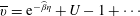 $\overline{v}=\text{e}^{-\widehat{\unicode[STIX]{x1D6FD}}\unicode[STIX]{x1D702}}+U-1+\cdots \,$
, constructed from (6.40)–(6.42). The numerical results are in excellent agreement with the asymptotic results when
$\overline{v}=\text{e}^{-\widehat{\unicode[STIX]{x1D6FD}}\unicode[STIX]{x1D702}}+U-1+\cdots \,$
, constructed from (6.40)–(6.42). The numerical results are in excellent agreement with the asymptotic results when
 $\widehat{\unicode[STIX]{x1D6FD}}\ll 1$
.
$\widehat{\unicode[STIX]{x1D6FD}}\ll 1$
.
Figure 11. Wall normal velocity profiles of the real parts of the Rayleigh solution as a function of the transverse Blasius coordinate
 $\unicode[STIX]{x1D702}$
for
$\unicode[STIX]{x1D702}$
for
 $M_{\infty }=3$
. (a) For small values of
$M_{\infty }=3$
. (a) For small values of
 $\widehat{\unicode[STIX]{x1D6FD}}$
(dashed curves denote uniformly valid composite solution constructed from (6.40)–(6.42). (b) For intermediate values of
$\widehat{\unicode[STIX]{x1D6FD}}$
(dashed curves denote uniformly valid composite solution constructed from (6.40)–(6.42). (b) For intermediate values of
 $\widehat{\unicode[STIX]{x1D6FD}}$
.
$\widehat{\unicode[STIX]{x1D6FD}}$
.
Table 2. Estimation of modified Rayleigh neutral point location for flight conditions at
 $M_{\infty }=3$
(
$M_{\infty }=3$
(
 $U_{\infty }^{\ast }=888~\text{m}~\text{s}^{-1}$
,
$U_{\infty }^{\ast }=888~\text{m}~\text{s}^{-1}$
,
 $\unicode[STIX]{x1D708}_{\infty }^{\ast }=0.000264~\text{m}^{2}~\text{s}^{-1}$
) at an altitude of 20 km.
$\unicode[STIX]{x1D708}_{\infty }^{\ast }=0.000264~\text{m}^{2}~\text{s}^{-1}$
) at an altitude of 20 km.

The Rayleigh equation (6.25) develops a critical layer when
 $\overline{\unicode[STIX]{x1D6FC}}$
becomes real, which occurs when
$\overline{\unicode[STIX]{x1D6FC}}$
becomes real, which occurs when
 $\widehat{\unicode[STIX]{x1D6FD}}\rightarrow 0$
. It follows from the expansion (6.30) that the critical layer moves toward the wall and lies at
$\widehat{\unicode[STIX]{x1D6FD}}\rightarrow 0$
. It follows from the expansion (6.30) that the critical layer moves toward the wall and lies at
 $\unicode[STIX]{x1D702}=\widehat{\unicode[STIX]{x1D6FD}}(T_{w}/\unicode[STIX]{x1D706})^{2}$
when
$\unicode[STIX]{x1D702}=\widehat{\unicode[STIX]{x1D6FD}}(T_{w}/\unicode[STIX]{x1D706})^{2}$
when
 $\widehat{\unicode[STIX]{x1D6FD}}\rightarrow 0$
. It eventually moves into the viscous wall layer when
$\widehat{\unicode[STIX]{x1D6FD}}\rightarrow 0$
. It eventually moves into the viscous wall layer when
 $\overline{x}_{1}=\mathit{O}(\unicode[STIX]{x1D716}^{2+r})$
. This corresponds to
$\overline{x}_{1}=\mathit{O}(\unicode[STIX]{x1D716}^{2+r})$
. This corresponds to
 $\hat{x}_{1}=\mathit{O}(\unicode[STIX]{x1D716}^{3r})\leqslant \mathit{O}(1)$
which will lie well within the triple-deck region for realistic values of
$\hat{x}_{1}=\mathit{O}(\unicode[STIX]{x1D716}^{3r})\leqslant \mathit{O}(1)$
which will lie well within the triple-deck region for realistic values of
 $\unicode[STIX]{x1D716}$
.
$\unicode[STIX]{x1D716}$
.
The present study can also be extended to two-dimensional mean flow boundary layers on slightly curved surfaces. And while the analysis is probably not relevant for the boundary layers on highly swept wings such as the ones on current subsonic transports, it is expected to be very relevant to boundary layer transition on the nearly straight wing on aircraft such as the low-sweep Aerion AS2 supersonic Bizjet, shown in figure 12 – especially for wind tunnel testing, where strong acoustic disturbances are generated on the wind tunnel walls.

Figure 12. Low-sweep Aerion AS2 supersonic Bizjet. Posted by Tim Brown on the manufacturer Newsletter.
The analysis is also easily extended to supersonic wedge flows. It would directly apply to the flow behind the leading edge shock if the free-stream disturbance downstream of the shock rather than the disturbance field upstream of the shock were taken as input. But the shock wave will now couple the acoustic and vortical (as well as the entropic) free-stream disturbances and the downstream boundary layer can even produce reflected acoustic disturbance, which, as shown by the theoretical analyses of Duck, Lasseigne & Hussaini (Reference Duck, Lasseigne and Hussaini1997) and Cowley & Hall (Reference Cowley and Hall1990), will not play a significant role in the moderate supersonic Mach number regime being considered in this paper. The simultaneous consideration of the acoustic and vortical free-stream disturbances is however essential in this case. And finally it should be noted that the F/K disturbances are expected to become more significant than the Lam–Rott disturbances at sufficiently high free-stream Mach numbers (say,
 $M_{\infty }>4$
) and/or sufficiently cold walls (for which
$M_{\infty }>4$
) and/or sufficiently cold walls (for which
 $T_{w}$
is smaller than the adiabatic wall temperature), where the growth rate of the second Mack mode becomes larger than that of the oblique first mode. In fact, the main purpose of the F/K analysis was to deal with such hypersonic cases.
$T_{w}$
is smaller than the adiabatic wall temperature), where the growth rate of the second Mack mode becomes larger than that of the oblique first mode. In fact, the main purpose of the F/K analysis was to deal with such hypersonic cases.
9 Concluding remarks
High Reynolds number asymptotics was used to study the non-local behaviour of boundary layer instabilities generated by small amplitude free-stream disturbances at moderate supersonic Mach numbers. The vortical disturbances produce an unsteady boundary flow that develops into oblique instability waves with a viscous triple-deck structure in the downstream region where the frequency-scaled streamwise coordinate
 $x$
is
$x$
is
 $\mathit{O}(\unicode[STIX]{x1D716}^{-2})$
. The analysis is analogous to the leading edge receptivity analysis carried by Goldstein (Reference Goldstein1983) in the incompressible limit, but the present results are expected to be much more robust because the instability waves now undergo very little decay before they begin to grow. F/K analysed the generation of inviscid instabilities in supersonic boundary layers by fast and slow acoustic disturbances in the free stream. They considered the case where the deviation
$\mathit{O}(\unicode[STIX]{x1D716}^{-2})$
. The analysis is analogous to the leading edge receptivity analysis carried by Goldstein (Reference Goldstein1983) in the incompressible limit, but the present results are expected to be much more robust because the instability waves now undergo very little decay before they begin to grow. F/K analysed the generation of inviscid instabilities in supersonic boundary layers by fast and slow acoustic disturbances in the free stream. They considered the case where the deviation
 $\unicode[STIX]{x0394}\unicode[STIX]{x1D703}\equiv \unicode[STIX]{x1D703}_{c}-\unicode[STIX]{x1D703}$
of the obliqueness angle from its critical value is
$\unicode[STIX]{x0394}\unicode[STIX]{x1D703}\equiv \unicode[STIX]{x1D703}_{c}-\unicode[STIX]{x1D703}$
of the obliqueness angle from its critical value is
 $\mathit{O}(1)$
and showed that downstream propagating slow acoustic disturbances with
$\mathit{O}(1)$
and showed that downstream propagating slow acoustic disturbances with
 $\unicode[STIX]{x0394}\unicode[STIX]{x1D703}>0$
generate unsteady boundary layer disturbances that match onto the inviscid 1st Mack instability mode when the frequency-scaled distance
$\unicode[STIX]{x0394}\unicode[STIX]{x1D703}>0$
generate unsteady boundary layer disturbances that match onto the inviscid 1st Mack instability mode when the frequency-scaled distance
 $x$
is
$x$
is
 $\mathit{O}(\unicode[STIX]{x1D716}^{-6})=\mathit{O}({\mathcal{F}}^{-1})$
which is much further downstream than the region where the viscous triple-deck instability emerges from the vortically generated unsteady boundary layer flow. But, as shown in § 8, this instability emerges too far downstream to be of interest when scaled up to actual flight conditions for the small incidence angle disturbances considered in this paper. However, the inviscid instability, which first appears at an
$\mathit{O}(\unicode[STIX]{x1D716}^{-6})=\mathit{O}({\mathcal{F}}^{-1})$
which is much further downstream than the region where the viscous triple-deck instability emerges from the vortically generated unsteady boundary layer flow. But, as shown in § 8, this instability emerges too far downstream to be of interest when scaled up to actual flight conditions for the small incidence angle disturbances considered in this paper. However, the inviscid instability, which first appears at an
 $\mathit{O}(\unicode[STIX]{x1D716}^{-(4+2r)})$
distance downstream when
$\mathit{O}(\unicode[STIX]{x1D716}^{-(4+2r)})$
distance downstream when
 $\unicode[STIX]{x0394}\unicode[STIX]{x1D703}$
is reduced to
$\unicode[STIX]{x0394}\unicode[STIX]{x1D703}$
is reduced to
 $\mathit{O}(\unicode[STIX]{x1D716}^{1-r})$
with
$\mathit{O}(\unicode[STIX]{x1D716}^{1-r})$
with
 $1/3\leqslant r<1$
, can be of considerable importance when scaled to flight conditions. It is therefore appropriate to compare the vortically generated instabilities with the instabilities generated by oblique acoustic disturbances with obliqueness angles in this range as is done in this paper. These acoustic disturbances generate slow boundary layer disturbances which eventually develop into oblique stable disturbances with inviscid triple-deck structure in a region that lies downstream of the viscous triple-deck region. The acoustically generated oblique F/K disturbances are therefore likely to be insignificant compared to the vortically generated Lam–Rott instabilities. The paper shows that both of these instabilities eventually develop into modified Rayleigh-type instabilities (which can either grow or decay) further downstream.
$1/3\leqslant r<1$
, can be of considerable importance when scaled to flight conditions. It is therefore appropriate to compare the vortically generated instabilities with the instabilities generated by oblique acoustic disturbances with obliqueness angles in this range as is done in this paper. These acoustic disturbances generate slow boundary layer disturbances which eventually develop into oblique stable disturbances with inviscid triple-deck structure in a region that lies downstream of the viscous triple-deck region. The acoustically generated oblique F/K disturbances are therefore likely to be insignificant compared to the vortically generated Lam–Rott instabilities. The paper shows that both of these instabilities eventually develop into modified Rayleigh-type instabilities (which can either grow or decay) further downstream.
The global Lam–Rott instabilities are low frequency disturbances that occur when the scaled frequency parameter
 $1/\overline{\unicode[STIX]{x1D6FD}}^{\dagger }$
is less than the critical value
$1/\overline{\unicode[STIX]{x1D6FD}}^{\dagger }$
is less than the critical value
 $1/0.978$
and the global F/K instabilities are high frequency disturbances that occur when
$1/0.978$
and the global F/K instabilities are high frequency disturbances that occur when
 $1/\overline{\unicode[STIX]{x1D6FD}}=1/\unicode[STIX]{x1D716}^{r}$
,
$1/\overline{\unicode[STIX]{x1D6FD}}=1/\unicode[STIX]{x1D716}^{r}$
,
 $1/3\leqslant r<1$
. Since
$1/3\leqslant r<1$
. Since
 $\unicode[STIX]{x1D716}^{1/3}$
could easily be equal to 0.978 numerically and since the leading edge shock wave can convert acoustic disturbance into convected disturbances, this may explain the results given in Fedorov (Reference Fedorov2003) which show that the F/K solution significantly underpredicts the experimental data of Maslov et al. (Reference Maslov, Shiplyuk, Sidorenko and Arnal2001) in the vicinity of the critical angle.
$\unicode[STIX]{x1D716}^{1/3}$
could easily be equal to 0.978 numerically and since the leading edge shock wave can convert acoustic disturbance into convected disturbances, this may explain the results given in Fedorov (Reference Fedorov2003) which show that the F/K solution significantly underpredicts the experimental data of Maslov et al. (Reference Maslov, Shiplyuk, Sidorenko and Arnal2001) in the vicinity of the critical angle.
Acknowledgements
This research was sponsored by NASA’s Transformational Tools and Technologies (TTT) Project of the Transformative Aeronautics Concepts Program under the Aeronautics Research Mission Directorate. P.R. acknowledges the financial support by the Air Force Office of Scientific Research award number AFOSR grant FA9550-15-1-0248. The authors would also like to thank Dr M. Choudhari for making them aware of the photograph in figure 12.
Appendix A. Rescaling of F/K solution for
$\unicode[STIX]{x0394}\unicode[STIX]{x1D703}\ll 1$

Inserting
 $$\begin{eqnarray}\tilde{\tilde{x}}_{2}\equiv \frac{x_{2}}{(\unicode[STIX]{x0394}\unicode[STIX]{x1D703})^{a}(\unicode[STIX]{x0394}\unicode[STIX]{x1D711})^{a_{1}}}=\mathit{O}(1)\end{eqnarray}$$
and
 $$\begin{eqnarray}\tilde{{\tilde{y}}}_{2}\equiv \frac{y_{2}}{(\unicode[STIX]{x0394}\unicode[STIX]{x1D703})^{b}(\unicode[STIX]{x0394}\unicode[STIX]{x1D711})^{b_{1}}}=\mathit{O}(1),\quad \tilde{k}\equiv k\unicode[STIX]{x0394}\unicode[STIX]{x1D711}\end{eqnarray}$$
 $$\begin{eqnarray}\displaystyle & \displaystyle \frac{1}{(\unicode[STIX]{x0394}\unicode[STIX]{x1D703})^{2b}(\unicode[STIX]{x0394}\unicode[STIX]{x1D711})^{2b_{1}}}\frac{\unicode[STIX]{x2202}^{2}p_{2}}{\unicode[STIX]{x2202}\tilde{{\tilde{y}}}_{2}^{2}}=\frac{2\text{i}\tilde{\unicode[STIX]{x1D6FC}}(M_{\infty }^{2}-1)}{(\unicode[STIX]{x0394}\unicode[STIX]{x1D711})^{a_{1}}(\unicode[STIX]{x0394}\unicode[STIX]{x1D703})^{a+1}}\frac{\unicode[STIX]{x2202}p_{2}}{\unicode[STIX]{x2202}\tilde{\tilde{x}}_{2}}, & \displaystyle\end{eqnarray}$$
 $$\begin{eqnarray}\displaystyle & \displaystyle \frac{1}{(\unicode[STIX]{x0394}\unicode[STIX]{x1D711})^{b_{1}}(\unicode[STIX]{x0394}\unicode[STIX]{x1D703})^{b-1}}\frac{\unicode[STIX]{x2202}p_{2}}{\unicode[STIX]{x2202}\tilde{{\tilde{y}}}_{2}}=-\text{i}\tilde{\unicode[STIX]{x1D6FC}}v_{1}(\infty ),\quad p_{2}=p_{1}(x_{2})\quad \text{at }y_{2}=0, & \displaystyle\end{eqnarray}$$
 $$\begin{eqnarray}\displaystyle & \displaystyle v_{1}(\infty )=\frac{\text{i}\tilde{\unicode[STIX]{x1D6FC}}\tilde{k}(\unicode[STIX]{x0394}\unicode[STIX]{x1D703})^{a/2}(\unicode[STIX]{x0394}\unicode[STIX]{x1D711})^{a_{1}/2}}{\unicode[STIX]{x0394}\unicode[STIX]{x1D711}\unicode[STIX]{x0394}\unicode[STIX]{x1D703}\cos ^{2}\unicode[STIX]{x1D703}}\left(\frac{\sqrt{2\tilde{\tilde{x}}_{2}}}{\tilde{\unicode[STIX]{x1D6FC}}\unicode[STIX]{x1D706}}\right)^{2/3}\sqrt{\tilde{\tilde{x}}_{2}}p_{2}. & \displaystyle\end{eqnarray}$$
These equations will therefore remain unchanged if we put
 $$\begin{eqnarray}2b=a+1,\quad 2b_{1}=a_{1},\quad b_{1}=1-a_{1}/2,\quad b-1=1-a/2\end{eqnarray}$$
and it follows that
 $$\begin{eqnarray}a={\textstyle \frac{3}{2}},\quad b={\textstyle \frac{5}{4}},\quad b_{1}={\textstyle \frac{1}{2}},\quad a_{1}=1\end{eqnarray}$$
and therefore that
 $\tilde{\tilde{x}}_{2}$
and
$\tilde{\tilde{x}}_{2}$
and
 $\tilde{{\tilde{y}}}_{2}$
are given by (4.28).
$\tilde{{\tilde{y}}}_{2}$
are given by (4.28).
Appendix B. Solution for the
$\unicode[STIX]{x0394}\unicode[STIX]{x1D703}=\mathit{O}(\unicode[STIX]{x1D716}^{2/3})$
viscous wall layer

The solution in the main boundary layer is given by (4.22) and (4.26). The solution in wall layer where
 $$\begin{eqnarray}\displaystyle & \displaystyle \tilde{\unicode[STIX]{x1D702}}\equiv \frac{\unicode[STIX]{x1D702}}{\unicode[STIX]{x0394}\unicode[STIX]{x1D711}}=\frac{y}{\unicode[STIX]{x1D716}^{3}\unicode[STIX]{x0394}\unicode[STIX]{x1D711}T_{w}\sqrt{2x}}=\frac{y}{T_{w}\unicode[STIX]{x1D716}^{15/8}(\unicode[STIX]{x0394}\unicode[STIX]{x1D703})^{27/16}\sqrt{2\tilde{\tilde{x}}_{2}}}=\mathit{O}(1), & \displaystyle\end{eqnarray}$$
 $$\begin{eqnarray}\displaystyle & \displaystyle Y\equiv \frac{y}{\unicode[STIX]{x1D716}^{3}[\unicode[STIX]{x0394}\unicode[STIX]{x1D703}/\unicode[STIX]{x1D716}^{2/3}]^{27/16}} & \displaystyle\end{eqnarray}$$
expands like
 $$\begin{eqnarray}\displaystyle \{u,v,w,p\} & = & \displaystyle \frac{\unicode[STIX]{x0394}\unicode[STIX]{x1D703}\unicode[STIX]{x1D706}\unicode[STIX]{x1D702}}{T_{w}\sqrt{2\tilde{\tilde{x}}_{2}}}+\frac{\hat{\unicode[STIX]{x1D6FF}}}{\unicode[STIX]{x0394}\unicode[STIX]{x1D703}}\left\{\overline{U}(\tilde{\tilde{x}}_{2},\tilde{\unicode[STIX]{x1D702}}),\left[\frac{\unicode[STIX]{x1D716}^{3}}{(\unicode[STIX]{x0394}\unicode[STIX]{x1D703})^{1/2}}\right]^{7/8}\overline{V}(\tilde{\tilde{x}}_{2},\tilde{\unicode[STIX]{x1D702}}),\overline{W}(\tilde{\tilde{x}}_{2},\tilde{\unicode[STIX]{x1D702}}),\right.\nonumber\\ \displaystyle & & \displaystyle \left.\unicode[STIX]{x0394}\unicode[STIX]{x1D703}p_{1}(\tilde{\tilde{x}}_{2})\vphantom{\left[\frac{\unicode[STIX]{x1D716}^{3}}{(\unicode[STIX]{x0394}\unicode[STIX]{x1D703})^{1/2}}\right]^{7/8}}\right\}\text{e}^{\text{i}(\unicode[STIX]{x1D6FC}x+\unicode[STIX]{x1D6FD}z-t)}.\end{eqnarray}$$
Inserting (B 3) along with (4.19) into the Navier–Stokes equations shows that
 $\overline{U}(\tilde{\tilde{x}}_{2},\tilde{\unicode[STIX]{x1D702}})$
,
$\overline{U}(\tilde{\tilde{x}}_{2},\tilde{\unicode[STIX]{x1D702}})$
,
 $\overline{V}(\tilde{\tilde{x}}_{2},\tilde{\unicode[STIX]{x1D702}})$
,
$\overline{V}(\tilde{\tilde{x}}_{2},\tilde{\unicode[STIX]{x1D702}})$
,
 $\overline{W}(\tilde{\tilde{x}}_{2},\tilde{\unicode[STIX]{x1D702}})$
satisfy
$\overline{W}(\tilde{\tilde{x}}_{2},\tilde{\unicode[STIX]{x1D702}})$
satisfy
 $$\begin{eqnarray}\displaystyle & \displaystyle \text{i}\tilde{\unicode[STIX]{x1D6FC}}\overline{U}+\frac{\unicode[STIX]{x2202}\overline{V}}{\unicode[STIX]{x2202}Y}+\text{i}\tilde{\unicode[STIX]{x1D6FD}}\overline{W}=0, & \displaystyle\end{eqnarray}$$
 $$\begin{eqnarray}\displaystyle & \displaystyle -\text{i}\left(1-\tilde{\unicode[STIX]{x1D6FC}}\frac{\unicode[STIX]{x1D706}Y}{T_{w}\sqrt{2\tilde{\tilde{x}}_{2}}}\right)\overline{U}+\frac{\unicode[STIX]{x1D706}}{T_{w}\sqrt{2\tilde{\tilde{x}}_{2}}}\overline{V}=-\text{i}\unicode[STIX]{x1D6FC}T_{w}p_{1}+\unicode[STIX]{x1D707}_{w}T_{w}\frac{\unicode[STIX]{x2202}^{2}\overline{U}}{\unicode[STIX]{x2202}Y^{2}}, & \displaystyle\end{eqnarray}$$
 $$\begin{eqnarray}\displaystyle & \displaystyle -\text{i}\left(1-\tilde{\unicode[STIX]{x1D6FC}}\frac{\unicode[STIX]{x1D706}Y}{T_{w}\sqrt{2\tilde{\tilde{x}}_{2}}}\right)\overline{W}=-\text{i}\tilde{\unicode[STIX]{x1D6FD}}T_{w}p_{1}+\unicode[STIX]{x1D707}_{w}T_{w}\frac{\unicode[STIX]{x2202}^{2}\overline{W}}{\unicode[STIX]{x2202}Y^{2}}, & \displaystyle\end{eqnarray}$$
subject to the boundary conditions
 $$\begin{eqnarray}\overline{U}\rightarrow -\frac{\unicode[STIX]{x1D706}\overline{A}}{T_{w}}+\frac{T_{w}^{2}\sqrt{2\tilde{\tilde{x}}_{2}}\tilde{\unicode[STIX]{x1D6FD}}^{2}p_{1}}{\tilde{\unicode[STIX]{x1D6FC}}^{2}\unicode[STIX]{x1D706}Y},\quad \overline{W}\rightarrow -\frac{\tilde{\unicode[STIX]{x1D6FD}}p_{1}T_{w}^{2}\sqrt{2\tilde{\tilde{x}}_{2}}}{\tilde{\unicode[STIX]{x1D6FC}}\unicode[STIX]{x1D706}Y}\quad \text{as }Y\rightarrow \infty ,\end{eqnarray}$$
 $$\begin{eqnarray}\overline{U}(0),\overline{V}(0),\overline{W}(0)=0,\end{eqnarray}$$
which upon introducing the variable
 $$\begin{eqnarray}\unicode[STIX]{x1D709}\equiv \unicode[STIX]{x1D709}_{0}+\overline{\unicode[STIX]{x1D709}},\end{eqnarray}$$
where
 $$\begin{eqnarray}\overline{\unicode[STIX]{x1D709}}\equiv Y\left(\frac{\text{i}\unicode[STIX]{x1D706}\tilde{\unicode[STIX]{x1D6FC}}T_{w}}{\unicode[STIX]{x1D707}_{w}\sqrt{2\tilde{\tilde{x}}_{2}}}\right)^{1/3}\end{eqnarray}$$
and
 $$\begin{eqnarray}\unicode[STIX]{x1D709}_{0}=-\text{i}^{1/3}\left(\frac{\sqrt{2\tilde{\tilde{x}}_{2}}}{\tilde{\unicode[STIX]{x1D6FC}}\unicode[STIX]{x1D706}}\right)^{2/3}\left(\frac{T_{w}}{\unicode[STIX]{x1D707}_{w}}\right)^{1/3},\end{eqnarray}$$
becomes
 $$\begin{eqnarray}\displaystyle & \displaystyle \unicode[STIX]{x1D709}\overline{W}=\tilde{\unicode[STIX]{x1D6FD}}T_{w}\unicode[STIX]{x1D709}_{0}p_{1}+\frac{\unicode[STIX]{x2202}^{2}\overline{W}}{\unicode[STIX]{x2202}\unicode[STIX]{x1D709}^{2}}, & \displaystyle\end{eqnarray}$$
 $$\begin{eqnarray}\displaystyle & \displaystyle \unicode[STIX]{x1D709}\frac{\unicode[STIX]{x2202}\overline{U}}{\unicode[STIX]{x2202}\unicode[STIX]{x1D709}}=\frac{\tilde{\unicode[STIX]{x1D6FD}}}{\tilde{\unicode[STIX]{x1D6FC}}}\overline{W}+\frac{\unicode[STIX]{x2202}^{3}\overline{U}}{\unicode[STIX]{x2202}\unicode[STIX]{x1D709}^{3}}, & \displaystyle\end{eqnarray}$$
 $$\begin{eqnarray}\overline{U}=0,\quad \overline{W}=0,\quad \frac{\unicode[STIX]{x2202}^{2}\overline{U}}{\unicode[STIX]{x2202}\unicode[STIX]{x1D709}^{2}}=-\tilde{\unicode[STIX]{x1D6FC}}T_{w}\unicode[STIX]{x1D709}_{0}p_{1}\quad \text{at }\unicode[STIX]{x1D709}=\unicode[STIX]{x1D709}_{0}.\end{eqnarray}$$
The solution to this problem, which is now pretty standard, is
 $$\begin{eqnarray}\overline{W}=-\unicode[STIX]{x03C0}\tilde{\unicode[STIX]{x1D6FD}}T_{w}\unicode[STIX]{x1D709}_{0}p_{1}\text{Gi}(\unicode[STIX]{x1D709}_{0})\left[\frac{\text{Ai}(\unicode[STIX]{x1D709})}{\text{Ai}(\unicode[STIX]{x1D709}_{0})}-\frac{\text{Gi}(\unicode[STIX]{x1D709})}{\text{Gi}(\unicode[STIX]{x1D709}_{0})}\right],\end{eqnarray}$$
 $$\begin{eqnarray}\overline{U}=\frac{\unicode[STIX]{x03C0}\tilde{\unicode[STIX]{x1D6FD}}^{2}T_{w}\unicode[STIX]{x1D709}_{0}p_{1}}{\tilde{\unicode[STIX]{x1D6FC}}}\text{Gi}(\unicode[STIX]{x1D709}_{0})\left[\frac{\text{Ai}(\unicode[STIX]{x1D709})}{\text{Ai}(\unicode[STIX]{x1D709}_{0})}-\frac{\text{Gi}(\unicode[STIX]{x1D709})}{\text{Gi}(\unicode[STIX]{x1D709}_{0})}\right]-p_{1}T_{w}\frac{(\tilde{\unicode[STIX]{x1D6FC}}^{2}+\tilde{\unicode[STIX]{x1D6FD}}^{2})\unicode[STIX]{x1D709}_{0}}{\tilde{\unicode[STIX]{x1D6FC}}\text{Ai}^{\prime }(\unicode[STIX]{x1D709}_{0})}\int _{\unicode[STIX]{x1D709}_{0}}^{\unicode[STIX]{x1D709}}\text{Ai}(q)\,\text{d}q,\end{eqnarray}$$
where
 $\text{Ai}$
and
$\text{Ai}$
and
 $\text{Gi}$
denote the Airy function and Airy function integral defined in Abramowitz & Stegun (Reference Abramowitz and Stegun1964, pp. 446 and 448).
$\text{Gi}$
denote the Airy function and Airy function integral defined in Abramowitz & Stegun (Reference Abramowitz and Stegun1964, pp. 446 and 448).
Matching with (4.22) and (4.23) shows that
 $$\begin{eqnarray}\tilde{A}\unicode[STIX]{x1D706}=p_{1}T_{w}^{2}\frac{(\tilde{\unicode[STIX]{x1D6FC}}^{2}+\tilde{\unicode[STIX]{x1D6FD}}^{2})\unicode[STIX]{x1D709}_{0}}{\tilde{\unicode[STIX]{x1D6FC}}\text{Ai}^{\prime }(\unicode[STIX]{x1D709}_{0})}\int _{\unicode[STIX]{x1D709}_{0}}^{\infty }\text{Ai}(\unicode[STIX]{x1D709})\,\text{d}\unicode[STIX]{x1D709}\end{eqnarray}$$
and, therefore, that the wall normal velocity
 $v(\tilde{\tilde{x}}_{2},\infty )\equiv \lim _{\unicode[STIX]{x1D702}\rightarrow \infty }v_{1}(\tilde{\tilde{x}}_{2},\unicode[STIX]{x1D702})$
is given by (4.29).
$v(\tilde{\tilde{x}}_{2},\infty )\equiv \lim _{\unicode[STIX]{x1D702}\rightarrow \infty }v_{1}(\tilde{\tilde{x}}_{2},\unicode[STIX]{x1D702})$
is given by (4.29).
Appendix C. Asymptotic solution to the diffraction region problem
Since the dominant contribution to the sum
 $$\begin{eqnarray}\ln a_{n}=\mathop{\sum }_{j=1}^{n}\ln \frac{\unicode[STIX]{x1D6E4}(4j/3+1/2)}{\unicode[STIX]{x1D6E4}(4j/3+1)}\end{eqnarray}$$
(obtained by taking the logarithm of (4.43)) comes from the terms with
 $j\geqslant j_{0}$
where
$j\geqslant j_{0}$
where
 $1\leqslant j_{0}\leqslant n$
when
$1\leqslant j_{0}\leqslant n$
when
 $n\gg 1$
, it follows from Abramowitz & Stegun (Reference Abramowitz and Stegun1964, equation (6.1.40)) that
$n\gg 1$
, it follows from Abramowitz & Stegun (Reference Abramowitz and Stegun1964, equation (6.1.40)) that
 $$\begin{eqnarray}\displaystyle \ln a_{n} & {\sim} & \displaystyle \mathop{\sum }_{j=j_{0}}^{n}\ln \frac{\unicode[STIX]{x1D6E4}(4j/3+1/2)}{\unicode[STIX]{x1D6E4}(4j/3+1)}\sim -\frac{1}{2}\mathop{\sum }_{j=j_{0}}^{n}\ln \left(\frac{4j}{3}\right)\sim -\frac{1}{2}\int _{j_{0}}^{n}\ln \left(\frac{4\unicode[STIX]{x1D702}}{3}\right)\text{d}\unicode[STIX]{x1D702}\nonumber\\ \displaystyle & {\sim} & \displaystyle -\frac{n}{2}\left[\ln \left(\frac{4n}{3}\right)-1\right]\end{eqnarray}$$
and, therefore, that
 $$\begin{eqnarray}a_{n}\sim A\left(\frac{3e}{4n}\right)^{n/2},\end{eqnarray}$$
where
 $A$
is a constant. Then since the main contribution to the series (4.41) comes from its infinite tail when
$A$
is a constant. Then since the main contribution to the series (4.41) comes from its infinite tail when
 $Z\rightarrow \infty$
, it follows that (Bender & Orszag Reference Bender and Orszag1999, pp. 376–379)
$Z\rightarrow \infty$
, it follows that (Bender & Orszag Reference Bender and Orszag1999, pp. 376–379)
 $$\begin{eqnarray}\displaystyle p_{1} & = & \displaystyle \mathop{\sum }_{n=0}^{\infty }a_{n}Z^{n}\sim \frac{A}{(2\unicode[STIX]{x03C0})^{1/4}}\mathop{\sum }_{n=N}^{\infty }\frac{(\text{e}^{1/2}Z)^{n}}{(4n/3)^{n/2}}\sim \frac{A}{(2\unicode[STIX]{x03C0})^{1/4}}\int _{T}^{\infty }\left(Z\sqrt{\frac{3e}{4t}}\right)^{t}\,\text{d}t\nonumber\\ \displaystyle & {\sim} & \displaystyle \frac{3AZ^{2}}{4(2\unicode[STIX]{x03C0})^{1/4}}\int _{4T/3Z^{2}}^{\infty }\left(\frac{e}{\unicode[STIX]{x1D70F}}\right)^{3\unicode[STIX]{x1D70F}Z^{2}/8}\,\text{d}\unicode[STIX]{x1D70F}\sim \frac{3AZ^{2}}{4(2\unicode[STIX]{x03C0})^{1/4}}\int _{0}^{\infty }\text{e}^{-(3\unicode[STIX]{x1D70F}Z^{2}/8)(\ln \unicode[STIX]{x1D70F}-1)}\,\text{d}\unicode[STIX]{x1D70F}.\end{eqnarray}$$
Then since the dominant contribution to this integral comes from the saddle point at
 $\ln \unicode[STIX]{x1D70F}=0$
, applying the method of steepest descent shows that
$\ln \unicode[STIX]{x1D70F}=0$
, applying the method of steepest descent shows that
 $p_{1}$
behaves like
$p_{1}$
behaves like
 $$\begin{eqnarray}p_{1}\sim \frac{3A}{4(2\unicode[STIX]{x03C0})^{1/4}}\sqrt{\frac{4\unicode[STIX]{x03C0}}{Z^{2}}}Z^{2}\text{e}^{3Z^{2}/8}=\frac{3AZ}{2}\left(\frac{\unicode[STIX]{x03C0}}{2}\right)^{1/4}\text{e}^{3Z^{2}/8}.\end{eqnarray}$$
Appendix D. Comparison with Ricco–Wu (2007) solution
Ricco & Wu (Reference Ricco and Wu2007) show that
 $$\begin{eqnarray}\int _{\unicode[STIX]{x1D709}_{0}}^{\infty }\text{Ai}(q)\,\text{d}q=(\text{i}\unicode[STIX]{x1D6FC})^{-1/3}\left[\frac{F^{\prime \prime }(0)}{\sqrt{2\tilde{x}_{1}}}\right]^{5/3}\left(\frac{\unicode[STIX]{x1D707}_{w}}{T_{w}^{7}}\right)^{1/3}\frac{[1-(M_{\infty }^{2}-1)(\unicode[STIX]{x1D6FC}_{1}{\hat{s}})^{2}]^{1/2}}{1+(\unicode[STIX]{x1D6FC}_{1}{\hat{s}})^{2}}\text{Ai}^{\prime }(\unicode[STIX]{x1D709}_{0}),\end{eqnarray}$$
 $$\begin{eqnarray}\tilde{x}_{1}=\frac{k_{3}x}{k_{1}}\sqrt{\frac{k_{1}}{R_{\unicode[STIX]{x1D6E5}}}},\quad \unicode[STIX]{x1D709}_{0}=-\text{i}^{1/3}\left[\frac{\sqrt{2\tilde{x}_{1}}}{\unicode[STIX]{x1D6FC}_{1}F^{\prime \prime }(0)}\right]^{2/3}\left(\frac{T_{w}}{\unicode[STIX]{x1D707}_{w}}\right)^{1/3}\end{eqnarray}$$
and
 $$\begin{eqnarray}{\hat{s}}\equiv \frac{k_{1}^{5/4}R_{\unicode[STIX]{x1D6E5}}^{1/4}}{k_{3}^{3/2}},\quad k_{1}\equiv \frac{\unicode[STIX]{x1D714}^{\ast }\unicode[STIX]{x1D6E5}^{\ast }}{U_{\infty }^{\ast }},\end{eqnarray}$$
where
 $\unicode[STIX]{x1D6E5}^{\ast }$
denotes their spanwise scale factor,
$\unicode[STIX]{x1D6E5}^{\ast }$
denotes their spanwise scale factor,
 $k_{3}$
denotes a scaled spanwise wavenumber and it follows from (2.13) and (2.14) that
$k_{3}$
denotes a scaled spanwise wavenumber and it follows from (2.13) and (2.14) that
 $$\begin{eqnarray}R_{\unicode[STIX]{x1D6E5}}\equiv \frac{U_{\infty }^{\ast }\unicode[STIX]{x1D6E5}^{\ast }}{\unicode[STIX]{x1D708}_{\infty }^{\ast }}\rightarrow \frac{k_{1}}{\unicode[STIX]{x1D716}^{6}}.\end{eqnarray}$$
Comparing (D 2)–(D 4) with (3.6), (4.6), and (5.12) of Ricco & Wu (Reference Ricco and Wu2007) shows that
 $$\begin{eqnarray}\frac{k_{3}}{k_{1}}\rightarrow \frac{\overline{\unicode[STIX]{x1D6FD}}}{\unicode[STIX]{x1D716}},\quad \unicode[STIX]{x1D6FC}_{1}\rightarrow \sqrt{\overline{\unicode[STIX]{x1D6FD}}}\unicode[STIX]{x1D705}_{0}.\end{eqnarray}$$
And it therefore follows that
 $$\begin{eqnarray}{\hat{s}}\unicode[STIX]{x1D6FC}_{1}\rightarrow \frac{\unicode[STIX]{x1D705}_{0}}{\overline{\unicode[STIX]{x1D6FD}}},\quad \tilde{x}_{1}\rightarrow \overline{\unicode[STIX]{x1D6FD}}x_{1}.\end{eqnarray}$$


