2. Geometry and flow conditions

For the numerical investigation presented here, the geometry and the flow conditions of the experiments at the AFRL Mach 6 High-Reynolds Number Facility were used (Jewell et al. Reference Jewell, Kennedy, Laurence and Kimmel2018). The geometry (see figure 2) is a $7^\circ$ half-angle straight (right) cone with a nose radius of $r_{{nose}} = 1.524\ \textrm {mm}$ ($0.06\ \textrm {in}$) corresponding to the $3\,\%$ bluntness case from Jewell et al. (Reference Jewell, Kennedy, Laurence and Kimmel2018). The flow conditions are summarized in table 1, and the case chosen is marked in figure 1 with a red dot. The fluid is considered to be a perfect gas with a constant Prandtl number ($Pr = 0.71$) and a constant ratio of specific heats ($\gamma = 1.4$), and the viscosity is calculated using the standard Sutherland's law (no low-temperature correction).

Figure 2. Schematic of the blunt-cone geometry.

Table 1. Flow conditions.

3. Simulation strategy

For the simulations presented here, a three-step strategy was employed that has been successfully used previously for stability investigations and ‘controlled’ breakdown DNS for different geometries and flow conditions (see for example Laible et al. Reference Laible, Mayer and Fasel2009; Hader & Fasel Reference Hader and Fasel2019). Step 1 consists of a precursor calculation to obtain the steady base flow around the entire geometry (including the nose) using either a finite-volume code developed in our CFD laboratory by Gross & Fasel (Reference Gross and Fasel2008) or CFD++ (Chakravarthy et al. Reference Chakravarthy, Peroomian, Goldberg and Palaniswamy1998). In step 2, a new base flow is calculated in a smaller subdomain using a high-order-accurate finite-difference code, which was also developed in our laboratory by Laible et al. (Reference Laible, Mayer and Fasel2009). In step 3, the actual stability and transition simulations are carried out in the same subdomain as for step 2 using the same high-order finite-difference code.

4. Base flow

Contours of Mach number and the density of the laminar base flow (figure 3) show the formation of a bow shock around the nose of the cone, resulting in a strong entropy layer. The inset in figure 3 indicates the entire size of the cone geometry as used in the experiments of Jewell & Kimmel (Reference Jewell and Kimmel2016). The area shaded with dark grey in figure 3 highlights the extent of the subdomain used for the stability and transition simulations presented here. A comparison of the boundary-layer thickness determined at the location where the total enthalpy reaches 99.5 % of the total free stream enthalpy ($h_{t}(\delta _{99.5})=0.995h_{t\infty }$) and the entropy-layer thickness ($\delta _S$) calculated using (${\rm \Delta} S(\delta _S)=0.25{\rm \Delta} S_{{wall}}$, $\Delta S = c_{p}ln(T/T_{\infty}) - R_{g}ln(p/p_{\infty})$ where $c_{p}$ and $R_{g}$ are the specific heat and gas constant of the fluid, respectively), as also used by Paredes et al. (Reference Paredes, Choudhari, Li, Jewell and Kimmel2019b), is shown in figure 4. Close to the nose, the entropy layer is very thick compared with the boundary layer. The entropy-layer thickness rapidly decreases in the downstream direction but is not ‘swallowed’. The edge Mach number ($M_e$ see figure 4) is drastically reduced compared with free stream Mach number due to the strong shock. For the entire computational domain, it remains well below $M_e = 4$.

Figure 3. Contours of Mach number (M) and density $(\rho)$ normalized with the free-stream density $(\rho_{\infty})$, and the cone geometry as used in the original experiments with the dark grey shaded area highlighting the size of the computational domain used here.

Figure 4. Development of the boundary layer and entropy-layer thickness $(\delta)$, and the edge Mach number in the downstream direction.

5. Linear and nonlinear stability investigations

5.1. Linear stability investigations

For a blunt flat plate at $M = 2.5$, Dietz & Hein (Reference Dietz and Hein1999) found amplified entropy-layer instabilities. Results from a LST analysis using our in-house developed linear stability solver (parallel flow assumptions, Haas Reference Haas2020) for the geometry and flow conditions considered here (table 1) are shown in figure 5. The location of the inflow and outflow boundaries of the computational domain that was used for the highly resolved ‘controlled’ breakdown DNS are highlighted in figure 5. No unstable disturbance waves in the computational domain considered here were found from the LST analysis. Note that in the same region unstable disturbance waves were also not found in the PSE analysis by Jewell et al. (Reference Jewell, Kennedy, Laurence and Kimmel2018). Therefore, ‘linear’ stability investigations were carried using DNS introducing small amplitude disturbances into the computational domain. Simulations by Husmeier & Fasel (Reference Husmeier and Fasel2007) showed that for a blunt cone at $M=8$ the flow field was most receptive to continuously forced disturbances in the entropy layer. Thus, for this ‘linear’ stability investigation, total energy perturbations were introduced into the entropy layer using a volume-forcing approach. Low resolution (in the azimuthal direction) calculations were carried out for a wide range of frequencies and azimuthal wavenumbers. The spatial growth rates extracted from these calculations are provided in figure 6(a). Close to the inflow of the computational domain, a region of substantial growth over a very short downstream distance for oblique waves ($k_c>0$) of all the frequencies considered here can be observed (figure 6a). This very large linear growth was neither captured with LST nor with PSE, likely due to the assumptions required in LST and PSE. The maximum growth rates were obtained for an azimuthal wavenumber of $k_c\approx 300$. Due to the large growth rates of these unstable disturbances, relatively large $N$-factors (up to approximately 20) are reached over a short downstream distance as can be observed in figure 6(b). The ‘linear’ results clearly indicate that only oblique waves are amplified, while the flow is stable for axisymmetric waves (figure 6).

Figure 5. Growth rates from LST (A. Haas, private communication) for a wide range of frequencies (f) and azimuthal wavenumbers $(k_c)$. The grey planes indicate the location of the inflow and outflow boundary of the computational domain used for the highly resolved DNS.

Figure 6. (a) Growth rates and (b) $N$-factors from ‘linear’ stability investigations using low amplitude DNS for a wide range of forcing frequencies and azimuthal wavenumbers with slices of constant frequency at $f=50$, $f =200$, $f=350$ and $f=500$ kHz.

5.2. Nonlinear stability investigations

The linear stability investigations have shown that oblique disturbances are amplified while axisymmetric ones are not. Therefore, fundamental or subharmonic resonance are likely not relevant in the computational domain considered here and for these flow conditions and nose bluntness. Consequently, the possibility of an oblique breakdown (Fasel et al. Reference Fasel, Thumm and Bestek1993) was investigated in detail. To allow for a possible future comparison with numerical investigations of the same geometry and flow conditions by Paredes et al. (Reference Paredes, Choudhari and Li2019a,Reference Paredes, Choudhari, Li, Jewell and Kimmelb), a pair of oblique disturbance waves with $f = 250$ kHz and an azimuthal wavenumber of $k_c=50$ was chosen. This disturbance wave was found to have large linear amplification rates (see figure 6) in our stability investigations using DNS. While Paredes et al. (Reference Paredes, Choudhari and Li2019a,Reference Paredes, Choudhari, Li, Jewell and Kimmelb) investigated the possibility of non-modal growth leading to transition, the very large linear amplification rates obtained from DNS are exploited here to rapidly trigger nonlinear interactions and a subsequent oblique breakdown. In order to find out if oblique breakdown can be initiated with the selected disturbance waves, an oblique breakdown onset study was carried out by forcing a pair of oblique disturbance waves ($f=250$ kHz, $k_c = \pm 50$) with successively increasing amplitudes. The instantaneous pressure disturbances on the surface of the cone in figure 7 show that for a forcing amplitude of $A_{0}=1\times 10^{-6}$ (figure 7, top) the disturbances are amplified after reaching the wall and the sinusoidal nature of the disturbances suggests that this is a purely ‘linear’ amplification. Increasing the forcing amplitude to $A_{0}=1\times 10^{-5}$ (figure 7, middle) results in a distortion of the sinusoidal waveform of the instantaneous disturbance signal that is caused by nonlinear effects. When forced with a sufficiently large amplitude ($A_{0}=5\times 10^{-5}$), a strong nonlinear distortion of the disturbance signal can be observed. This suggests that an oblique breakdown (Fasel et al. Reference Fasel, Thumm and Bestek1993) may be a relevant nonlinear mechanism.

Figure 7. Instantaneous pressure disturbances $(p')$ normalized with twice the dynamic pressure, where $U_{\infty}$ is the freestream velocity, at the wall for three different forcing amplitudes $(A_0)$.

6. Oblique breakdown

In the simulation set-up for the nonlinear transition investigation by Paredes et al. (Reference Paredes, Choudhari, Li, Jewell and Kimmel2019b), non-modal disturbances (obtained from linear non-modal analysis, and ‘blown-up’ to large ‘nonlinear’ amplitudes) are forced at the inflow boundary of their computational domain. Thus, the nonlinear development resulting from that particular forcing is specific to what is imposed at the inflow as a boundary condition, in their case, a pair of non-modal oblique disturbances with $k_c=50$, $f=250$ kHz (Note that in Paredes et al. (Reference Paredes, Choudhari, Li, Jewell and Kimmel2019b) the azimuthal wavenumber is denoted with m). In contrast, our simulation set-up was motivated by the landmark ‘controlled’ boundary-layer transition experiments by Schubauer & Skramstad (Reference Schubauer and Skramstad1948), which validated the LST for the primary instability. Furthermore, it is motivated by the subsequent ‘controlled’ transition experiments by Klebanoff, Tidstrom & Sargent (Reference Klebanoff, Tidstrom and Sargent1962), which set the stage for the development of the secondary instability theory for incompressible boundary layers. In these experiments, local but ‘controlled disturbances’ of specified frequencies and amplitudes were introduced (via a ‘vibrating ribbon’). Thus, in these landmark experiments, the receptivity of the flow with respect to the ‘actuator’ (vibrating ribbon) was included in the flow response. These ‘controlled’ transition experiments laid the foundation for the understanding of low-speed boundary-layer transition.

The simulations discussed in our paper are set up in the spirit of these landmark low-speed ‘controlled’ transition experiments as hypersonic experimental equivalents have not yet been carried out. Towards this end, in our simulations, the disturbances are deliberately not forced at the inflow, but rather, as in the above mentioned experiments, locally (in our case in the entropy layer) using ‘controlled disturbances’ (with respect to amplitude, frequency and azimuthal wavenumber), so that the ‘actuator’ receptivity to the employed forcing is also included. Therefore, the resulting nonlinear transition mechanisms are not driven by imposed streamwise modes at the inflow boundary as in Paredes et al. (Reference Paredes, Choudhari, Li, Jewell and Kimmel2019b), but rather, the oblique transition mechanisms are allowed to ‘play out freely’ without any bias, and the streamwise modes are nonlinearly generated and can participate in the nonlinear transition process. It should be noted that a local ‘controlled’ disturbance generation as used in the present simulations could be realized in future high-speed transition experiments.

With the forcing parameters determined as discussed above, a highly resolved so-called ‘controlled’ oblique breakdown DNS was carried out. Towards this end, a pair of oblique disturbance waves with a frequency of $f=250$ kHz and an azimuthal wavenumber of $k_c=\pm 50$ were introduced into the entropy layer with an amplitude of $A_{0}=5\times 10^{-5}$. The computational domain for this simulation was focused on a region close to the blunted nose of the cone geometry (see figure 3). In the streamwise direction, the computational domain was resolved with $n_x=6800$ grid points with the inflow boundary located at $x=0.025$ m and the outflow at $x=0.125$ m. The grid spacing was refined in the downstream direction in order to resolve all relevant length scales near the downstream end of the domain where the nonlinear breakdown stages will be reached. The shock-fitted grid extends up to the shock location which was obtained from precursor calculations. A total of $n_{\eta }=698$ grid points clustered near the wall and in the entropy layer were used in the wall-normal direction. The computational domain in the azimuthal direction ($0\ \textrm {rad} \leq \varphi \leq {\rm \pi}/50\ \textrm {rad}$) was resolved with $n_{\varphi } = 199$ grid points (100 Fourier modes). For the wall-normal direction, grid convergence studies were carried (not presented here for brevity) to ensure that the boundary layer and the entropy layer were sufficiently resolved. An a priori estimate of the wall units was obtained with the turbulent skin-friction estimates (White Reference White2006). Based on these estimates, the grid line distribution was designed such that in the wall-normal direction ${\rm \Delta} y^+ \approx 1$ was obtained in the entire computational domain, and ${\rm \Delta} x^+<5$ was used in the refined region in the downstream direction where nonlinear breakdown was expected based on the oblique breakdown onset calculations (see § 5).

Contours of the instantaneous temperature disturbance in the symmetry plane from the nonlinear oblique breakdown DNS are shown in figure 8. For reference, the entropy-layer ($\delta _S$) and boundary-layer ($\delta _{99.5}$) thicknesses of the laminar base flow are also provided in figure 8. The oblique disturbance waves initially propagate along the entropy layer (figure 8a). The spatial forcing function used for the volume force was a so-called ‘monopole’ in the streamwise and the wall-normal direction. This shape is initially ‘imprinted’ on the disturbance waves but shortly downstream of the forcing location the disturbance waves adjust and exhibit an elongated shape ‘slanted’ upwards (figure 8a). A detailed view of the entropy-layer structures downstream of the forcing location (figure 8b) shows that the main structures are developing above the boundary layer. The ‘tails’ of these structures begin to penetrate the boundary layer (figure 8b) and then quickly become stretched in the streamwise direction due to the reduced flow speed inside of the boundary layer (figure 8c). While the structures comprising positive temperature disturbance values remain nearly unchanged, the structures that penetrated into the boundary layer (negative temperature disturbances) quickly merge and contaminate the entire boundary layer (figure 8d). Farther downstream, the ‘tail’ of the large structures in the entropy layer descends into the boundary layer and smaller scales are generated (figure 8d), indicating that the flow is progressing deeper into the nonlinear breakdown regime. Towards the end of the computational domain, the flow exhibits a breakdown to very small structures that are characteristic for a turbulent boundary layer. Remnants of the entropy-layer structures can still be observed even long after the nonlinear stages of the laminar-turbulent transition process have been reached. Thus, these ‘coherent’ structures persist far into the late stages of the transition process and into the turbulent boundary layer. The instantaneous three-dimensional structures of the late stages of the nonlinear transition process in figure 9 confirm that the coherent structures in the entropy layer prevail downstream into the late nonlinear transition stages. The negative temperature disturbances are layered between the wall and the positive temperature disturbances in the entropy layer.

Figure 8. Contours of the instantaneous temperature disturbance $(T')$ normalized with the free-stream temperature $(T_{\infty})$ in the symmetry plane.

Figure 9. Isosurfaces of the instantaneous three-dimensional temperature disturbances in the turbulent breakdown region.

The downstream development of the pressure disturbance amplitude extracted at the wall (figure 10a) and the maximum pressure disturbance amplitude (figure 10b) provide insight into which nonlinear interactions are dominating the transition process. For convenience, the notation $(n,m)$ which is a shorthand notation for $(n\times f_{{forced}},m\times k_{c,{domain}})$, where $f_{forced}$ is the frequency of the forced disturbance wave and $k_{c,domain}$ is the smallest azimuthal wavenumber resolved in the computational domain has been adopted here (for details see Hader & Fasel Reference Hader and Fasel2019). For the results presented here, the normalization parameters are $f_{{forced}} = 250$ kHz and $k_{c,{domain}}=50$. The development of the pressure disturbance amplitude at the wall (figure 10a) indicates that initially all modes are decaying downstream of the forcing location until a strong exponential (linear in the log plot) growth sets in, quickly leading to very large amplitudes for a wide range of disturbance waves at $x\approx 0.087$. Thereupon the oblique forced mode $(1,1)$ and all nonlinearly generated modes reach peak values. Thereafter, surprisingly, the disturbances decay until $x\approx 0.095$ m, from whereon all disturbance waves experience strong amplification, in particular the higher frequencies and azimuthal wavenumbers (indicated with grey lines, figure 10). The modes highlighted in colour (figure 10) are the so-called ‘signature modes’ of the oblique breakdown (Fasel et al. Reference Fasel, Thumm and Bestek1993), thus providing evidence that oblique breakdown is indeed the dominant nonlinear mechanism. These observations are the same for the development of the maximum pressure disturbance amplitudes (figure 10b). The most notable difference is that the amplification of the forced mode $(1,1)$ at the wall (figure 10a) sets in farther upstream (at approximately $x\approx 0.05$ m) compared with the development of the maximum pressure disturbance amplitude (at approximately $x\approx 0.07$ m, figure 10b).

Figure 10. Downstream development of the pressure disturbance amplitude at the wall $(p'_{wall})$ (a), and the maximum pressure disturbance amplitude (b).

As can be observed in figure 10(b), the streamwise mode (0,2), as well as the other signature modes of oblique breakdown, are generated as a consequence of a nonlinear interaction of the oblique modes (1,1) and (1,$-$1) which are the only ‘controlled’ disturbances introduced into the flow due to the simulation set-up as discussed above. This is in contrast to the numerical investigations of Paredes et al. (Reference Paredes, Choudhari, Li, Jewell and Kimmel2019b), where the streamwise modes were already introduced at the inflow of the computational domain by using disturbances obtained from a non-modal stability calculation.

The azimuthal wavenumber of the forced oblique waves was $k_c = 50$, resulting in a steady streamwise mode $(0,2)$ with $k_c = 100$. In the non-modal analysis by Paredes et al. (Reference Paredes, Choudhari, Li, Jewell and Kimmel2019b), a steady streamwise mode with $k_c = 100$ exhibits the largest N-factor. In the DNS for the ‘controlled’ oblique breakdown, not only steady streamwise modes but also a wide range of other modes are nonlinearly generated, in particular also the so-called ‘signature modes’ (see figure 10), which in turn can lead to other levels of nonlinear interactions. Therefore, it is difficult to establish an unambiguous link between the nonlinearly generated steady streamwise modes observed in the present oblique breakdown DNS and the steady streamwise modes obtained from the transient growth analysis by Paredes et al. (Reference Paredes, Choudhari, Li, Jewell and Kimmel2019b). Our simulations seem to indicate that the nonlinear breakdown is not only associated with the secondary instability of the steady streamwise modes, as described by Berlin, Lundbladh & Henningson (Reference Berlin, Lundbladh and Henningson1994) for incompressible flows, but is rather also caused by the rapid and strong nonlinear interactions with all the other unsteady, nonlinearly generated disturbances (see figure 10).

Contours of the time-averaged Stanton number on the surface of the cone are displayed in figure 11(a). Towards the end of the computational domain, streaks of increased Stanton number (‘hot streaks’) begin to develop. The streak spacing in the azimuthal direction is ${\rm \Delta} \varphi = 2{\rm \pi} /100$ or exactly 100 streaks around the circumference of the cone. The streak spacing corresponds to the azimuthal wavenumber of the steady streamwise mode (0,2), which is nonlinearly generated by interaction of the forced oblique modes $(1,\pm 1)$. Farther downstream these streaks merge in the azimuthal direction resulting in an increased Stanton number around the entire circumference of the cone, indicating that the flow has progressed deep into the nonlinear breakdown regime. The development of the Stanton number in the downstream direction extracted at different azimuthal locations is displayed in figure 11(b), where the laminar and turbulent estimates for a sharp cone (shifted in the downstream direction to the virtual cone origin of a perfectly sharp cone) are provided for reference. The Stanton number extracted along the streaks ($\varphi =0$, $\varphi ={\rm \pi} /100$ rad) shows a rapid deviation from the laminar estimate towards the turbulent value around $x\approx 0.09$ m. The Stanton number extracted at an azimuthal location between the streaks (figure 11(b), $\varphi ={\rm \pi} /50$ rad) exhibits a delayed deviation from the laminar value. At $x\approx 0.11$ m, the Stanton number has approached turbulent values at all azimuthal locations, and is later exceeding them (‘overshoot’) for some spanwise locations.

Figure 11. Contours of the time-averaged Stanton number $(C_h)$ on the surface of the cone (a), and development of the Stanton number in the downstream direction (b).

To provide a qualitative comparison to Schlieren images shown in Kennedy et al. (Reference Kennedy, Jagde, Laurence, Jewell and Kimmel2019), contours of ‘pseudo-schlieren’ are plotted in the symmetry plane in figure 12. As for the instantaneous temperature disturbance contours (figure 8), the entropy-layer thickness ($\delta _S$) and the boundary-layer thickness ($\delta _{99.5}$) are also provided in figure 12. The shape of the structures in the entropy layer that was observed in the instantaneous contours of the temperature disturbance (see figure 8) can also be seen in the ‘pseudo-schlieren’ (figure 12). As these ‘slanted’ structures propagate in the downstream direction their ‘tail’ begins to penetrate the boundary layer (figure 12b). The previously ‘quiet’ boundary layer is then quickly contaminated with the disturbances from the entropy layer and breakdown to small scales can be observed (figure 12d). This is followed by a rapid transition of the boundary layer while the coherent entropy-layer structures persist even in the late stages of the laminar-turbulent transition process (figure 12f). The small scales observed in the contours of the magnitude of the density gradient in figure 12(f) again confirm that the nonlinear stages of transition have been reached, and the flow is approaching turbulence.

Figure 12. Qualitative comparison of the Schlieren images taken from Kennedy et al. (Reference Kennedy, Jagde, Laurence, Jewell and Kimmel2019) (a,c,e) with ‘pseudo-schlieren’ (normalized magnitude of the density gradient, where $L_{ref} = 1\ \textrm{m}$ is the reference length scale used here) obtained from the oblique breakdown DNS (b,d,f).

The question arises how far transition has progressed towards fully turbulent flow. This can be addressed by analysing the van Driest transformed velocity profiles from the time-averaged flow field for different downstream and azimuthal locations (figure 13). The viscous sublayer and the log-layer are given as reference as a black dashed line and a dash-dotted line, respectively, in figure 13. The azimuthal locations at which the profiles were extracted correspond to a location cutting through the streaks ($\varphi =0$ rad) and between the streaks ($\varphi ={\rm \pi} /100$ rad). At $x=0.06$ m, the van Driest profiles (figure 13) at the two different azimuthal locations are indistinguishable from one another, thus the flow is most likely still laminar at this location. The profiles deviate from one another at $x=0.082$ m (figure 13) without any noticeable development of a log-layer. The profiles in the symmetry plane begin to approach the log-layer at $x=0.1$ m, while the profile between the streaks still appears to be laminar. Shortly downstream at $x=0.11$ and $x=0.12$ m (figure 13), the profiles at both azimuthal directions show the development of a log-layer, indicating that in this case the laminar-turbulent transition process is extremely rapid, resulting in a very short transition region. Here, the transition region is defined as the distance from the location where the Stanton number begins to deviate from its laminar value to where it has reached a sustained turbulent value. This rapid transition is in contrast to the findings for ‘controlled’ breakdown DNS for sharp straight and flared cones (see for example Laible et al. Reference Laible, Mayer and Fasel2009; Hader & Fasel Reference Hader and Fasel2019) where the transition region covered large portions of the geometry.

Figure 13. Van Driest transformed velocity $(u_c^+)$ profiles from the oblique breakdown simulations.

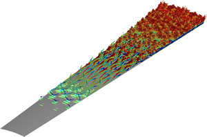
The instantaneous flow structures from the oblique breakdown simulation are visualized in figure 14 using $Q$-isocontours coloured with the contours of the instantaneous temperature disturbance. The isocontours of the $Q$-criterion confirm that the flow is laminar (no vortical structures) for a large downstream portion of the computational domain, followed by an explosive breakdown to turbulence towards the downstream end of the computational domain. The close-ups in figure 14 provide details of the laminar-turbulent breakdown process. The top down view (figure 14) shows the formation of staggered lambda vortices. At the downstream end of the computational domain, the flow has broken down to small scales, providing further evidence the boundary layer has reached the late stages of the transition process and the onset of turbulent flow.

Figure 14. Instantaneous isosurfaces of $Q=100\,000$ coloured with contours of the instantaneous temperature disturbance.