2.1 Linear stability analysis

Before considering the evolution of nonlinear wave interactions at the interface of a two-layer plane Couette–Poiseuille flow, it is instructive to briefly review the relevant linear theory.

2.1.1 Laminar linear stability analysis

Following the classical two-dimensional linear analysis of Yih (Reference Yih1967), the velocity and pressure variables are decomposed into as

(2.1) $$\begin{eqnarray}\left.\begin{array}{@{}c@{}}u_{j}=\hat{u} _{j}(x,z,t)+U_{j}(z)\\ w_{j}={\hat{w}}_{j}(x,z,t)\\ p_{j}=\hat{p}_{j}(x,z,t)+P(x)\end{array}\right\}\end{eqnarray}$$

for $j=1$ and 2, where $U_{j}(z)$ is the steady-state mean-velocity profile and $P(x)$ is the applied mean pressure across the channel. The fluctuating terms are then expanded in terms of the small variable $\unicode[STIX]{x1D716}$ (defined as the interfacial wave steepness), $\{\hat{u} _{j},{\hat{w}}_{j},\hat{p}_{j}\}=\unicode[STIX]{x1D716}\{\tilde{u} _{j},\tilde{w}_{j},\tilde{p}_{j}\}$ , and are substituted into the Navier–Stokes equations and interfacial and wall boundary conditions, which at leading order produce linearized equations of motion. The two-dimensional continuity equation permits the use of a stream function formulation, for which $\{\tilde{u} _{j},\tilde{w}_{j}\}=\{\unicode[STIX]{x1D713}_{j,z},-\unicode[STIX]{x1D713}_{j,x}\}$ , with the subscripts following the comma denoting partial differentiation. Assuming a travelling wave disturbance for all perturbation terms allows the flow variables to be expressed as $\{\unicode[STIX]{x1D713}_{j},\tilde{p}_{j},\tilde{\unicode[STIX]{x1D702}}\}=\{\unicode[STIX]{x1D719}_{j}(z),f_{j}(z),\unicode[STIX]{x1D702}_{o}\}\text{e}^{\text{i}k(x-ct)}$ , for which $c=c_{r}+ic_{i}$ is a complex number. This analysis produces the well-known Orr–Sommerfeld equations for each fluid

(2.2a ) $$\begin{eqnarray}\displaystyle {\mathcal{L}}_{1}\{\unicode[STIX]{x1D719}_{1}\} & \equiv & \displaystyle [(D^{2}-k^{2})^{2}-\text{i}k\,Re\{(U_{1}-c)(D^{2}-k^{2})-U_{1}^{\prime \prime }\}]\unicode[STIX]{x1D719}_{1}(z)=0\end{eqnarray}$$

(2.2b ) $$\begin{eqnarray}\displaystyle {\mathcal{L}}_{2}\{\unicode[STIX]{x1D719}_{2}\} & \equiv & \displaystyle \left[(D^{2}-k^{2})^{2}-\frac{\text{i}kr\,Re}{n}\{(U_{2}-c)(D^{2}-k^{2})-U_{2}^{\prime \prime }\}\right]\unicode[STIX]{x1D719}_{2}(z)=0,\end{eqnarray}$$

where $D$ denotes differentiation with respect to the $z$ -variable, $r=\unicode[STIX]{x1D70C}_{2}/\unicode[STIX]{x1D70C}_{1}$ , $n=\unicode[STIX]{x1D707}_{2}/\unicode[STIX]{x1D707}_{1}$ , $h=d_{2}/d_{1}$ , $Re=\unicode[STIX]{x1D70C}_{1}{\mathcal{U}}d_{1}/\unicode[STIX]{x1D707}_{1}$ is the Reynolds number and with ${\mathcal{L}}_{1}$ being defined over $z\in (0,1)$ and ${\mathcal{L}}_{2}$ being defined over $z\in (-h,0)$ . This problem is made complete with the accompanying wall (no-slip and no-flux) and interfacial boundary conditions (continuity of $u$ , $w$ and the normal and tangential stresses)

(2.3a ) $$\begin{eqnarray}\displaystyle & \displaystyle \frac{\text{d}}{\text{d}z}\unicode[STIX]{x1D719}_{1}(1)=0 & \displaystyle\end{eqnarray}$$

(2.3b ) $$\begin{eqnarray}\displaystyle & \displaystyle \frac{\text{d}}{\text{d}z}\unicode[STIX]{x1D719}_{2}(-h)=0 & \displaystyle\end{eqnarray}$$

(2.3c ) $$\begin{eqnarray}\displaystyle & \displaystyle \unicode[STIX]{x1D719}_{1}(1)=0 & \displaystyle\end{eqnarray}$$

(2.3d ) $$\begin{eqnarray}\displaystyle & \displaystyle \unicode[STIX]{x1D719}_{2}(-h)=0 & \displaystyle\end{eqnarray}$$

(2.3e ) $$\begin{eqnarray}\displaystyle & \displaystyle \unicode[STIX]{x1D719}_{1}(0)=\unicode[STIX]{x1D719}_{2}(0)\equiv \unicode[STIX]{x1D719}(0) & \displaystyle\end{eqnarray}$$

(2.3f ) $$\begin{eqnarray}\displaystyle & \displaystyle (c-U_{1}(0))\unicode[STIX]{x1D719}_{1}^{\prime }(0)+U_{1}^{\prime }(0)\unicode[STIX]{x1D719}_{1}(0)=(c-U_{2}(0))\unicode[STIX]{x1D719}_{2}^{\prime }(0)+U_{2}^{\prime }(0)\unicode[STIX]{x1D719}_{2}(0) & \displaystyle\end{eqnarray}$$

(2.3g ) $$\begin{eqnarray}\displaystyle & \displaystyle \unicode[STIX]{x1D719}_{1}^{\prime \prime }(0)+k^{2}\unicode[STIX]{x1D719}_{1}(0)=n(\unicode[STIX]{x1D719}_{2}^{\prime \prime }(0)+k^{2}\unicode[STIX]{x1D719}_{2}(0)) & \displaystyle\end{eqnarray}$$

(2.3h ) $$\begin{eqnarray}\displaystyle & & \displaystyle \frac{\text{i}k\,Re\unicode[STIX]{x1D719}(0)}{c-U_{1}(0)}[k^{2}S+{\mathcal{F}}]\nonumber\\ \displaystyle & & \displaystyle \quad =n(D^{3}\unicode[STIX]{x1D719}_{2}-3k^{2}\unicode[STIX]{x1D719}_{2}^{\prime })+\text{i}kr\,Re[(c-U_{2}(0))\unicode[STIX]{x1D719}_{2}^{\prime }+U_{2}^{\prime }(0)\unicode[STIX]{x1D719}_{2}]\nonumber\\ \displaystyle & & \displaystyle \qquad -\,(D^{3}\unicode[STIX]{x1D719}_{1}-3k^{2}\unicode[STIX]{x1D719}_{1}^{\prime })-\text{i}k\,Re[(c-U_{1}(0))\unicode[STIX]{x1D719}_{1}^{\prime }+U_{1}^{\prime }\unicode[STIX]{x1D719}_{1}],\end{eqnarray}$$

where ${\mathcal{F}}\equiv ((r-1)/Fr^{2})$ (with $Fr^{2}\equiv ({\mathcal{U}}^{2}/gd_{1})$ being the traditional square of the Froude number), $S\equiv (\unicode[STIX]{x1D6FE}/\unicode[STIX]{x1D70C}_{1}d_{1}{\mathcal{U}}^{2})$ being the dimensionless surface tension coefficient (and is equivalent to the reciprocal of the standard Weber number), and the $(~)^{\prime }$ denoting differentiation with respect to $z$ . Together, equations (2.2) and (2.3) define an eigenvalue problem for the eigenfunctions $\unicode[STIX]{x1D719}_{j}(z)$ and eigenvalue (wave speed) $c$ . This eigenvalue problem is solved using a modified form of the Chebyshev collocation (pseudospectral) method developed by Boomkamp & Miesen (Reference Boomkamp and Miesen1996). A detailed discussion of the numerical method is described in appendix A.

2.2 Nonlinear wave–wave resonances

A well-known property of linear systems is that waves of different wavelengths (frequencies) travel independently in space/time; however, when nonlinear wave interactions are accounted for, higher-order locked waves are generated. If the frequency and wavenumber of this locked wave satisfy the dispersion relationship, it becomes a free wave and undergoes what is referred to as resonant interactions. Under these conditions, the free wave component may grow significantly larger than when it is a locked wave, and can become of comparable amplitude to that of the primary waves. Studies, such as that of Phillips (Reference Phillips1960), have shown that resonant wave interactions have an important role in the evolution of ocean surface waves, and can result in significant energy transfer across the wave spectrum.

In this work, we examine the wave dynamics that occurs when a triad of resonantly interacting waves propagate on the interface of a two-fluid flow while at least one of the wave components is unstable to the linear Orr–Sommerfeld instability. For linearly stable systems, the amplitude of the interacting waves is usually bounded by the energy of their initial conditions; however, we will show that a triad of waves with one mode being linearly unstable can exhibit significantly larger long-term wave growth. Throughout the majority of this paper, we will focus on a triad composed of three wavenumbers with $k_{1}>k_{2}$ (with $k_{1}$ being the linearly unstable wave component). These three resonant waves must have wavenumbers and frequencies that satisfy

(2.4) $$\begin{eqnarray}\displaystyle \left.\begin{array}{@{}c@{}}k_{1}-k_{2}-k_{3}=0\\ \text{Re}\{\unicode[STIX]{x1D714}_{1}-\unicode[STIX]{x1D714}_{2}-\unicode[STIX]{x1D714}_{3}\}=\unicode[STIX]{x1D70E},\end{array}\right\} & & \displaystyle\end{eqnarray}$$

with $\unicode[STIX]{x1D70E}$ representing the frequency detuning and $\text{Re}$ denoting the real part of the expression. Note that the triad resonance condition is satisfied exactly when $\unicode[STIX]{x1D70E}=0$ . A special case of the triad resonance occurs when $k_{3}\rightarrow k_{2}$ . This case, referred to as a subharmonic resonance, has the corresponding resonance condition expressed as

(2.5) $$\begin{eqnarray}\displaystyle \left.\begin{array}{@{}c@{}}k_{1}-2k_{2}=0\\ \text{Re}\{\unicode[STIX]{x1D714}_{1}-2\unicode[STIX]{x1D714}_{2}\}=\unicode[STIX]{x1D70E}.\end{array}\right\} & & \displaystyle\end{eqnarray}$$

This class of resonances allows energy from the $k_{1}$ mode to be transferred to a second component with half the wavenumber (twice the wavelength). While this is merely a special case of the triad resonance, clear and pronounced subharmonic resonances are known to occur in nature, and are worth special consideration.

4.1 Initial condition

The Chebyshev spectral solution of the two-fluid Orr–Sommerfeld problem discussed in appendix A provides accurate approximations for the eigensolution (stream functions and wave speeds) and is used to develop the initial conditions for our numerical simulations.

The Orr–Sommerfeld analysis is derived by utilizing Taylor series expansions of the solution around the interface, allowing for the functions to be evaluated at $z=0$ rather than $z=\unicode[STIX]{x1D702}(x,t)$ , and results in the upper and lower eigenfunctions being calculated within the domain $z\in [0,1]$ and $z\in [-h,0]$ , respectively. The initial condition used by the Navier–Stokes solver contains a deformed interface corresponding to $z=\unicode[STIX]{x1D702}(x,t)$ . Therefore, the eigensolution is modified to produce an initial velocity field that accurately conforms to the deformed interfacial position by utilizing an algebraic mapping that transforms a rectangular domain to one with a wavy interface. The advantage of this algebraic mapping is that it preserves the velocity divergence condition while preserving the continuity of the normal velocity of the interface.

Consider the lower fluid in the Orr–Sommerfeld problem. The Chebyshev solution is defined on the domain of $(\hat{x},\hat{z})\in [0,L_{x}]\times [-h,0]$ , while the physical wavy solution has a domain defined on $(x,z)\in [0,L_{x}]\times [-h,\unicode[STIX]{x1D702}(x,z)]$ . The coordinate transformation

(4.1a ) $$\begin{eqnarray}\displaystyle \hat{x} & = & \displaystyle x\end{eqnarray}$$

(4.1b ) $$\begin{eqnarray}\displaystyle \hat{z} & = & \displaystyle h\frac{z-\unicode[STIX]{x1D702}(x,t)}{\unicode[STIX]{x1D702}(x,t)+h}\end{eqnarray}$$

(4.2a,b ) $$\begin{eqnarray}u_{1}(x,z)=\frac{\unicode[STIX]{x2202}\unicode[STIX]{x1D713}}{\unicode[STIX]{x2202}z},\quad u_{2}(x,z)=-\frac{\unicode[STIX]{x2202}\unicode[STIX]{x1D713}}{\unicode[STIX]{x2202}x}.\end{eqnarray}$$

For a given Chebyshev approximation of the stream function $\unicode[STIX]{x1D713}(\hat{x},\hat{z})$ , the transformation given by (4.1) allows the eigenfunctions within the wavy domain to be obtained through the derivative transformations, resulting in the perturbed velocity fields of the form

(4.3a ) $$\begin{eqnarray}\displaystyle u_{1}(x,z) & = & \displaystyle \frac{h}{h+\unicode[STIX]{x1D702}}\frac{\unicode[STIX]{x2202}\unicode[STIX]{x1D713}}{\unicode[STIX]{x2202}\hat{z}}\end{eqnarray}$$

(4.3b ) $$\begin{eqnarray}\displaystyle u_{2}(x,z) & = & \displaystyle -\left[\frac{\unicode[STIX]{x2202}\unicode[STIX]{x1D713}}{\unicode[STIX]{x2202}\hat{x}}+\frac{h(h+z)}{(\unicode[STIX]{x1D702}+h)^{2}}\frac{\unicode[STIX]{x2202}\unicode[STIX]{x1D702}}{\unicode[STIX]{x2202}x}\frac{\unicode[STIX]{x2202}\unicode[STIX]{x1D713}}{\unicode[STIX]{x2202}\hat{z}}\right].\end{eqnarray}$$

(4.4a ) $$\begin{eqnarray}\displaystyle \hat{x} & = & \displaystyle x\end{eqnarray}$$

(4.4b ) $$\begin{eqnarray}\displaystyle \hat{z} & = & \displaystyle \frac{z-\unicode[STIX]{x1D702}(x,t)}{1-\unicode[STIX]{x1D702}(x,t)},\end{eqnarray}$$

(4.5a ) $$\begin{eqnarray}\displaystyle u_{1}(x,z) & = & \displaystyle \frac{1}{1-\unicode[STIX]{x1D702}}\frac{\unicode[STIX]{x2202}\unicode[STIX]{x1D713}}{\unicode[STIX]{x2202}\hat{z}}\end{eqnarray}$$

(4.5b ) $$\begin{eqnarray}\displaystyle u_{2}(x,z) & = & \displaystyle -\left[\frac{\unicode[STIX]{x2202}\unicode[STIX]{x1D713}}{\unicode[STIX]{x2202}\hat{x}}-\frac{(1-z)}{(\unicode[STIX]{x1D702}-1)^{2}}\frac{\unicode[STIX]{x2202}\unicode[STIX]{x1D702}}{\unicode[STIX]{x2202}x}\frac{\unicode[STIX]{x2202}\unicode[STIX]{x1D713}}{\unicode[STIX]{x2202}\hat{z}}\right].\end{eqnarray}$$

4.2 Direct numerical simulation of Couette flow wave resonances

In this section, unstable triad resonant interactions in a Couette flow are considered. The two-layer wall-driven Couette flow (scaled by the dimensional interface velocity) has an initial (unperturbed) time-averaged mean-velocity profile

(4.6) $$\begin{eqnarray}U(z)=\left\{\begin{array}{@{}ll@{}}nz/h+1,\quad & z\in [0,1]\\ z/h+1,\quad & z\in [-h,0].\end{array}\right.\end{eqnarray}$$

The simplicity of this problem, combined with the harmonic averaging method for the interfacial shear stress model employed by the numerical algorithm, allows the mean-velocity profile to be simulated exactly.

Without carrying out the complete multiscale perturbation analysis, it is hard to know in advance how strong the nonlinear interactions will be. For this case, a grid search was carried out over the parameter space to identify the flow conditions for which there would be a strong interfacial instability and a strong triad resonance (indicated by $|\unicode[STIX]{x1D70E}|\ll 1$ ). Using the flow conditions, $r=100$ , $n=0.1818$ and $h=0.15$ , along with $Re=300$ , ${\mathcal{F}}=1$ , $S=3.5731\times 10^{-5}$ , analysis of linear Orr–Sommerfeld frequency spectrum identifies a resonant triad composed of $\{k_{1},k_{2},k_{3}=k_{1}-k_{2}\}=\{5,4,1\}$ with wave frequencies $\unicode[STIX]{x1D714}_{1}=0.8283+0.0747i$ , $\unicode[STIX]{x1D714}_{2}=0.7767-0.2962i$ , $\unicode[STIX]{x1D714}_{3}=0.0697-0.0319i$ . These three frequencies produce a resonant detuning parameter $\unicode[STIX]{x1D70E}=\text{Re}\{\unicode[STIX]{x1D714}_{1}-\unicode[STIX]{x1D714}_{2}-\unicode[STIX]{x1D714}_{3}\}\approx -0.0181$ .

Two-dimensional direct numerical simulations of these three resonantly interacting waves are carried out on the domain $(x,z)\in [0,2\unicode[STIX]{x03C0}]\times [-h,1]$ with $N_{x}\times N_{z}=1024^{2}$ grid points. Using the mapped eigenfunction method described in § 4.1, an initial condition is constructed through superposition of the three modal solutions. For the first set of simulations, the initial amplitudes are semi-arbitrarily chosen to be $a_{1}\equiv a_{k_{1}}=10^{-3}$ , $a_{2}\equiv a_{k_{2}}=5\times 10^{-4}$ , and $a_{3}\equiv a_{k_{3}}=10^{-5}$ . The only imposed constraints are that $a_{3}$ needs to have a small enough initial amplitude in order to accentuate this mechanism’s efficiency at long-wave generation, and $a_{1}$ needs to be small enough to have a sufficiently long period of clear linearly unstable growth.

The location of the interface is estimated from the VOF volume fraction by utilizing the mean value theorem of calculus. For a fixed $(x,y)$ -position, summing $f(x,y,z)\unicode[STIX]{x0394}z$ over the range of $z$ provides a measure of the depth of the upper fluid (which is indicated by $f=1$ ), while summing $[1-f(x,y,z)]\unicode[STIX]{x0394}z$ over the range of $z$ estimates the depth of the lower fluid (which is indicated by $f=0$ ). Therefore, after shifting this quantity by the equilibrium liquid depth $h$ , we obtain a second-order approximation of the interfacial elevation, which is denoted by $\unicode[STIX]{x1D702}(x_{i},y_{j},t)=\unicode[STIX]{x1D6F4}_{k}[1-f(x_{i},y_{j},z_{k})]\unicode[STIX]{x0394}z-h$ .

The time evolution of the nonlinearly interacting wave modes is shown in figure 2. Initially, all modes show excellent agreement with linear theory (depicted with the dashed lines), with $a_{1}$ growing due to the Orr–Sommerfeld instability and $a_{2},a_{3}$ being linearly damped. Due to the small amplitude of the $a_{3}$ -mode, it is most quickly impacted by the resonant interaction between the other two modes. As $a_{1}$ grows, it begins to transfer energy to the lightly damped $a_{3}$ mode, causing it to depart from linear theory at $t\sim O(3)$ and grow. Simultaneously, energy is transferred to the damped $a_{2}$ mode; however, no significant deviation from linear theory is observed, due to the strong damping rate. As $a_{1}$ and $a_{3}$ grow, they eventually reach an amplitude for which the nonlinear energy transfer to $a_{2}$ is able to overcome the linear damping. This causes it to depart from the theoretical linear solution and begin to grow around $t\sim O(15)$ . As all three modes continue to grow, the nonlinear interactions cause energy to be transferred among the interacting components. With $a_{1}$ being strongly unstable, it is not strongly impacted, but eventually the energy transfer from $a_{1}$ and $a_{3}$ allows $a_{2}$ to grow rapidly and overtake $a_{3}$ . However, after this occurs at $t\sim O(25)$ , the growth rate of $a_{3}$ increases and will likely cause it to overtake $a_{2}$ again. This exchange of energy is expected to continue until all three modes are of comparable order, at which point strong oscillations would likely occur among all three modes (as is typically the case in stable resonant interaction theory). For the current simulation, $|\unicode[STIX]{x1D70E}|\sim O(0.01)$ , and has been shown to present with strong nonlinear interactions. In the limit of $\unicode[STIX]{x1D70E}\rightarrow 0$ , the strength of the nonlinear interactions increases, causing the rate of energy transfer to increase and generate even more rapid wave growth.

Figure 2. Time evolution of the amplitudes of three resonantly interacting wave components. The plotted curves represent the simulation results for $a_{1}$ (- - - -), $a_{2}$ (

),  $a_{3}$ (— ⋅ —), and the linear theory prediction (——).

It is important to confirm that, during the initial stage of the simulation when $a_{2}$ and $a_{3}$ are decaying, the resulting departure from linear theory is indeed due to nonlinear interactions and not from a loss of numerical accuracy at these small scales. To confirm our findings, a second simulation is carried out with larger initial amplitudes, with $a_{1}=10^{-2}$ , $a_{2}=5\times 10^{-3}$ and $a_{3}=10^{-4}$ . The resulting time evolution of the modal amplitudes is shown in figure 3. The nonlinear interactions between the three modes cause the results to be amplitude dependent and the larger initial amplitudes result in stronger nonlinear forcing in this new case. As a result, similar characteristic features are observed, but the stronger nonlinear resonant forcing causes the modal growth of $a_{2}$ and $a_{3}$ to occur over a shorter time interval. The lightly damped $a_{3}$ mode is once again the first to depart from linear theory, followed by the strongly damped $a_{2}$ mode. All three modes then continue to grow and resonantly exchange energy amongst each other. It is important to note that in this case with the larger initial amplitude, the minimum value of $a_{2}$ is larger than in the previous case. This indicates that the behaviour change is due to the interaction and not due to numerical inaccuracy. This point is further exemplified in figure 4, which shows separate simulations of each individual wave component without any resonant exchange. All three components are plotted in the same figure to simplify the comparison with the resonant trial in figure 2. Each mode is in excellent agreement with the theoretical solution. Without the nonlinear resonant forcing, $a_{2}$ and $a_{3}$ only present with steady exponential decay, and are well represented by linear theory.

Figure 3. Time evolution of the amplitudes of three resonantly interacting wave components with larger initial amplitudes. The plotted curves represent the simulation results for $a_{1}$ (- - - -), $a_{2}$ (

),  $a_{3}$ (— ⋅ —) and the linear theory prediction (——).

In figures 2 and 3, the resonant modes present with weak oscillations around their theoretical solutions. These oscillations may occur for two different reasons. The first reason has to do with resolving the very small amplitude wave motions. Consider the $a_{2}$ mode shown in figure 2 for $t\sim O(7{-}15)$ . The initial amplitude of the $a_{2}$ component was $O(10^{-4})$ . During the initial phase of the simulation, its amplitude reduces by nearly two orders of magnitude and becomes very small. This small amplitude may cause minor numerical errors in the phase relationship between the interfacial waves and the velocity fluctuations. These discrepancies can result in small deviations in the linear growth rate and produce the weak oscillations around the theoretical solution. Second, previous studies by Campbell (Reference Campbell2009) used numerical simulations to show that, for linearly stable triads, resonant detuning and higher-order nonlinear wave interactions can lead to weak higher-frequency oscillations of the resonant modes around their theoretical amplitudes. These effects are generally weak (as shown by the $a_{1}$ mode in figure 3 for $t>O(3)$ ) and are overcome once the other resonant triad components become sufficiently large and the resonant energy exchange dominates the modal behaviour.

Figure 4. Time evolution of the individual $(k_{1},k_{2},k_{3})$ Orr–Sommerfeld wave component (without resonant interaction with other wave components). The plotted curves represent the simulation results for $a_{1}$ (- - - -), $a_{2}$ (

),  $a_{3}$ (— ⋅ —), and the linear theory prediction (——).

5.1 Problem description

The experiments carried out by Jurman et al. (Reference Jurman, Deutsch and McCready1992) consist of shear-generated interfacial waves in a co-current gas–liquid flow propagating through a small rectangular channel. In each case, the flow consists of a turbulent gas, with a mean gas $Re\sim O(4000{-}6300)$ , flowing over a laminar liquid layer, with a mean liquid $Re\sim O(5{-}70)$ . Several experiments are carried out over a range of flow conditions, and the resulting wave spectra show a wide range of interesting and distinct spectral behaviours.

Our original intention is to carry out direct numerical simulations at these experimental operating conditions due to the low (numerically resolvable) Reynolds numbers. Since these experiments are designed to capture marginally unstable wave growth, excessive computational run times are required to simulate these cases. To overcome this limitation, we use flow conditions similar to those reported in the experiments of Jurman et al. (Reference Jurman, Deutsch and McCready1992) (i.e. figure 7), but instead adjust the operating conditions (Reynolds numbers and liquid depths) to generate waves with stronger linear instabilities.

Therefore, in this work, we consider a turbulent (incompressible) gas flowing over a shallow laminar liquid layer. Scaling by the gas density, viscosity, equilibrium depth, and ${\mathcal{U}}=\sqrt{(d_{g}/\unicode[STIX]{x1D70C}_{g})|(\text{d}P/\text{d}x)|}$ results in a dimensionless applied pressure gradient of minus one and a Reynolds number of $Re\equiv \unicode[STIX]{x1D70C}_{1}{\mathcal{U}}d_{1}/\unicode[STIX]{x1D707}_{1}=533.21$ , along with the remaining dimensionless governing parameters $h\equiv d_{2}/d_{1}=0.26$ , $Fr^{2}=0.57$ , $r\equiv \unicode[STIX]{x1D70C}_{2}/\unicode[STIX]{x1D70C}_{1}=833.33$ , $n\equiv \unicode[STIX]{x1D707}_{2}/\unicode[STIX]{x1D707}_{1}=555.55$ and $S=0$ . The effects of surface tension are ignored in this simulation in order to achieve larger linear growth rates. The initially flat interface separating the two fluids is allowed to freely evolve under the influence of the turbulent forcing from a naturally occurring interfacial instability. In order to capture the nonlinear interfacial evolution under the influence of a turbulent gas blowing over a laminar liquid layer, an accurate turbulent gas field must be generated as the initial condition to this problem. Therefore, the simulations carried out in this section are broken into two separate phases. The first set of simulations is dedicated to developing accurate initial conditions of a statistically steady (fully developed) turbulent gas field which blows over a laminar liquid layer. The second set of simulations takes this initial condition and examine the fully nonlinear freely deforming interface between the two fluids.

5.2 Generation of initial turbulent flow

The first phase of the simulation is dedicated to developing an accurate turbulent initial condition that is used later during the second stage that carries out the nonlinear evolving interface trials. The strategy for developing this initial condition is constrained by several requirements. First, given that one of the primary objectives of this work is to observe which wavelengths become unstable under the influence of turbulent forcing, it is necessary for the interface to remain flat $(\unicode[STIX]{x1D702}(\boldsymbol{x},t)=0)$ during the initial turbulent development phase. Second, since the liquid flow is laminar, with $Re_{L}\sim O(10)$ , special attention is paid to the generation of the initial turbulent gas field such that it does not corrupt the liquid layer and result in its transition to turbulence.

Therefore, to generate a fully developed turbulent gas field while preserving the interface and laminar liquid properties, the following numerical strategy is developed. The initial condition is first set to the two-fluid laminar Poiseuille velocity and pressure profiles given by

(5.1a ) $$\begin{eqnarray}\displaystyle u & = & \displaystyle \left\{\begin{array}{@{}ll@{}}\displaystyle \frac{Re}{2n}\frac{\text{d}\bar{p}}{\text{d}x}z^{2}+\mathbb{C}_{1}z+\mathbb{C}_{2},\quad & z\in [-h,0]\\ \displaystyle \frac{Re}{2}\frac{\text{d}\bar{p}}{\text{d}x}z^{2}+\mathbb{C}_{3}z+\mathbb{C}_{4},\quad & z\in [0,1]\end{array}\right.\end{eqnarray}$$

(5.1b ) $$\begin{eqnarray}\displaystyle p & = & \displaystyle \left\{\begin{array}{@{}ll@{}}\displaystyle -\frac{r}{Fr^{2}}(z+h),\quad & z\in [-h,0]\\ \displaystyle -\frac{1}{Fr^{2}}(z+rh),\quad & z\in [0,1],\end{array}\right.\end{eqnarray}$$

(5.2) $$\begin{eqnarray}\left.\begin{array}{@{}l@{}}\displaystyle \mathbb{C}_{1}=-\frac{\text{d}\bar{p}}{\text{d}x}\frac{Re(n-h^{2})}{2n(n+h)},\quad \mathbb{C}_{3}=n\mathbb{C}_{1}\\ \displaystyle \mathbb{C}_{2}=-\frac{\text{d}\bar{p}}{\text{d}x}\frac{Reh(1+h)}{2(n+h)},\quad \mathbb{C}_{4}=\mathbb{C}_{2},\end{array}\right\}\end{eqnarray}$$

where $h\equiv d_{2}/d_{1}$ , $r\equiv \unicode[STIX]{x1D70C}_{2}/\unicode[STIX]{x1D70C}_{1}$ , and $n\equiv \unicode[STIX]{x1D707}_{2}/\unicode[STIX]{x1D707}_{1}$ . In order to prevent the turbulent transition of the liquid layer, the problem is adjusted to that of a single-phase pressure-driven Couette flow between two rigid walls. The upper wall remains stationary, while the lower wall moves horizontally (in the positive $x$ -direction) at the interface velocity of the two fluids given by (5.1a ). Reformulating the problem from a two-phase to a single-phase flow reduces the computational cost and ensures that the interface remains flat while the gas layer reaches a fully developed state. By requiring that the lower wall moves at the interface velocity, this method implicitly enforces that the liquid layer is laminar and will therefore be well conditioned for the next stage of two-phase simulations. Comparisons against the turbulent velocity profiles from Naraigh et al. (Reference Naraigh, Spelt, Matar and Zaki2011) show this to be a good approximation. Converting the initial turbulence generation problem to that of a single-phase flow also has the added benefit of not requiring that the initial round of simulations complies with the small two-fluid VOF time-step constraint (Weymouth & Yue Reference Weymouth and Yue2010, (21)) and allows the simulations to run with a larger time step based off of a single-fluid formulation.

In order to force the velocity field to transition to turbulence, a random divergence-free velocity field (whose magnitude is $O(10\,\%)$ of the maximum velocity of the laminar mean flow) is superposed on the initial laminar velocity field. Initially, this random velocity field is not representative of the proper turbulent statistics. However, by allowing the numerical algorithm to have a ‘warm-up’ period to evolve, the velocity field forces the transition to turbulence, and allows the turbulent fluctuations to recover physically realistic statistical distributions.

The length of the computational domain in the $x$ -direction and $y$ -direction is chosen to be large enough such that the two-point correlation of the energy spectra would decay to zero for large separation values. Once an accurate fully developed turbulent velocity field was generated, a linear stability analysis was used to confirm that all unstable wavenumbers are resolved within the domain. Additionally, a resonance analysis was also carried out to identify the longest resonant mode and ensure that the domain is sufficiently long to capture it. For all cases, the grid spacing in the $z$ -direction is selected such that there are a few points within the viscous sublayer. For the structured uniform grid used by this numerical method, the first point is located at a distance of $z^{+}=\unicode[STIX]{x0394}z^{+}/2$ from the interface and wall. A summary of the relevant computational parameters used in this simulation is listed in table 1.

Table 1. Computational parameters used in the direct numerical simulations where the $(\unicode[STIX]{x0394}x,\unicode[STIX]{x0394}y,\unicode[STIX]{x0394}z)^{+}=(\unicode[STIX]{x0394}x,\unicode[STIX]{x0394}y,\unicode[STIX]{x0394}z)u_{\ast i}/\unicode[STIX]{x1D708}_{u}$ .

To generate an accurate initial turbulent field, the initial solution is integrated forward in time until the velocity field reaches a statistically steady state (identified by a linear profile of the total stress). Once this condition is satisfied, the velocity field is integrated further in time in order for a time average of various statistical quantities to be determined. Based on the viscous length scale $\unicode[STIX]{x1D6FF}_{\ast }=\unicode[STIX]{x1D708}_{u}/u_{\ast i}$ and the interfacial friction velocity $u_{\ast i}=\sqrt{\unicode[STIX]{x1D70F}_{i}/\unicode[STIX]{x1D70C}_{u}}$ , a dimensionless time scale $t_{\ast }=(\unicode[STIX]{x1D6FF}_{\ast }/d_{1})({\mathcal{U}}/u_{\ast i})$ is used to guide the selection of the sample rate for the time averaging. In this paper, a sampling rate of $\unicode[STIX]{x0394}t=0.01$ is used. To improve the volume of statistical samples, all quantities are averaged over the horizontal planes ( $x$ and $y$ ). Therefore, for the remainder of this section, all $\overline{(~)}$ refer to quantities that are averaged over $x$ , $y$ and $t$ , while $(~)^{\prime }$ refers to turbulent fluctuations.

Using this numerical treatment, the resulting profiles of the turbulent mean flow, made dimensionless by the interfacial- and wall-shear velocities, are shown in figures 5(a) and 5(b), respectively. The dashed line represents the law of the wall and the log-law profiles. Within the interfacial and wall (denoted by the subscripts $i$ and $w$ respectively) viscous sublayers, $z_{i}^{+},z_{w}^{+}<5$ , the numerical results follow the linear law of the wall profiles given by $u_{i}^{+}=\overline{U}(0){\mathcal{U}}/u_{\ast i}+z^{+}$ and $u_{w}^{+}=z^{+}$ , where $u_{\ast i}=(\unicode[STIX]{x1D70F}_{i}/\unicode[STIX]{x1D70C}_{u})^{1/2}$ . Excellent agreement is observed. In the log-law region, the computational results are in agreement with the logarithmic velocity profile with $u_{i/w}^{+}=(1/\unicode[STIX]{x1D705})\log z^{+}+B_{i/w}$ , with $\unicode[STIX]{x1D705}=0.41$ being the von Kármán constant and the constants $B_{i}=6.5$ and $B_{w}=6$ , respectively. The mean of the $v$ - and $w$ -velocity components, denoted as $\overline{V}$ and $\overline{W}$ , respectively, are calculated and averaged, resulting in $\max |\overline{V}|\sim O(0.01)$ and $\max |\overline{W}|\sim O(10^{-14})$ . While $\overline{V}\ll 1$ , as expected, its non-zero magnitude is a numerical artefact due to the sampling frequency used for the time averaging.

Figure 5. Mean-velocity profile for (a) interfacial region and (b) wall region: numerical simulation (○) and asymptotic approximation (- - -) for viscous sublayer and log layers. Note that in (a) the mean velocity approaches the interface velocity as $z_{i}^{+}\rightarrow 0$ , while in (b) the mean velocity approaches zero (due to the stationary wall boundary condition) as $z_{w}^{+}\rightarrow 0$ .

Additional mean flow parameters are computed to assess the quality of the mean-velocity profile. The wall stress, normalized by the interfacial stress, is of the form

(5.3) $$\begin{eqnarray}-\frac{\unicode[STIX]{x1D70F}_{w}}{\unicode[STIX]{x1D70F}_{i}}=1+\frac{\text{d}\bar{P}}{\text{d}x}\frac{d_{1}}{\unicode[STIX]{x1D70F}_{i}}=1-\left(\frac{Re}{Re_{\ast i}}\right)^{2}.\end{eqnarray}$$

Numerically evaluating the interfacial and wall stress along with the Reynolds number based on the interfacial friction velocity $Re_{\ast i}$ produces the effective Reynolds number $Re_{e}=532.11$ , which is in close agreement with the prescribed Reynolds number of $Re=533.21$ . The small error in the computed interfacial and wall stresses results in approximately 0.2 % error in the Reynolds number. Additionally, the bulk mean velocity, defined as

(5.4) $$\begin{eqnarray}U_{mean}=\frac{1}{d_{1}}\int _{0}^{d_{1}}\bar{U}\,\text{d}z\end{eqnarray}$$

is calculated as well as the maximum velocity $(U_{max})$ . A summary of the resulting computed parameters is reported in table 2. Additional validation and examination of the initial turbulent solution is well documented in Campbell (Reference Campbell2015).

Table 2. Characterization of the time-averaged streamwise velocity profile.

5.3 Nonlinear interfacial evolution of turbulent gas–laminar liquid flow

The turbulent velocity field developed in the previous section is used as an initial condition to the two-fluid nonlinear evolving interface problem. For this second stage of the simulation, the solution is adjusted to run on a domain spanning $(x,y,z)\in [0,L_{x}]\times [0,L_{y}]\times [-h,1]$ and grid spacing $(\unicode[STIX]{x0394}x,\unicode[STIX]{x0394}y,\unicode[STIX]{x0394}z)=(L_{x}/N_{x},L_{y}/N_{y},(1+h)/N_{z})$ , with $(L_{x},L_{y},h)$ being defined in table 1. With this numerical grid, the turbulent field and fluid interface are sufficiently well resolved to observe the formation and evolution of the instability–resonance mechanism. This is confirmed in several different ways. First, the theoretical growth-rate spectrum, which is presented in § 5.3.2, shows that the dominant unstable energy of the spectrum is contained among the wavenumbers $k_{x}<15$ . Even if we conservatively consider resonant wavenumbers up to $k_{x}=30$ , the numerical mesh has a horizontal resolution that resolves this small wavelength with approximately nine grid points per wavelength. Second, the initial condition discussed in § 5.2 was calculated on a mesh which resolved the fields well into the viscous sublayer, and the mean-velocity profile is in excellent agreement with the asymptotic viscous sublayer and log-layer models. Furthermore, the results that are presented in the following sections are shown to be in close agreement with the linear stability analysis, and present with interfacial features that are consistent with those observed in physical experiments.

The initial velocity and pressure fields are defined such that the liquid layer is governed by the laminar fields given by (5.1), while the gas layer is given by the direct numerical simulations’ turbulent velocity and pressure field. Trilinear interpolation is used to transfer the turbulent solution from the single-phase domain to this new two-phase domain. The manner in which the initial single-phase turbulent gas field is generated ensures that the current interpolated initial condition satisfies the proper velocity and pressure continuities at the interface.

5.3.1 Nonlinear wave-field evolution

Using these flow conditions, the nonlinear time evolution of the interface is examined and the presence of resonant wave interactions is identified. The interfacial position is calculated every $\unicode[STIX]{x0394}t=0.02$ from the VOF volume fraction distribution using a second-order approximation given by $\unicode[STIX]{x1D702}(x_{i},y_{j},t)=\unicode[STIX]{x1D6F4}_{k}[1-f(x_{i},y_{j},z_{k})]\unicode[STIX]{x0394}z-h$ .

Figure 6. Time evolution of the interfacial elevation at (a) $t=0.2209$ , (b) $t=23.253$ , (c) $t=44.9588$ , (d) $t=71.7444$ , (e) $t=100.3539$ , and (f) $t=127.0727$ . Note that (a,b) share a common colour-bar range while (c–f) share a different common colour-bar range.

Figure 6 shows the time evolution of the interface under the influence of the turbulent gas blowing over a laminar liquid layer. At $t=0$ , the interface is perfectly flat with $\unicode[STIX]{x1D702}(x,y,t=0)=0$ . As the simulation begins, the turbulent fluctuations interact with the interface, generating small-amplitude high-wavenumber streamwise and cross-stream perturbations, as shown in figure 6(a). Continued interaction between gas turbulence and fluid interface causes the perturbations to slowly turn into long streaks with strong cross-stream variations which propagate in the streamwise direction, as shown in figure 6(b). Eventually, the natural interfacial instability(ies) cause the interface to transition from small-amplitude noise to a spectrum of two-dimensional wave disturbances, as shown in figure 6(c). This transition from noise to the two-dimensional fluctuations results in these two-dimensional perturbations being the dominant interfacial wave features, as shown in figure 6(d). Despite the strong growth and dominance of these two-dimensional wave components, the presence of weak cross-stream fluctuations prevents the interface from developing into purely monochromatic wave trains.

As the unstable wave components become steep, the interface eventually becomes bounded by nonlinearity, which results in the transition from the high-wavenumber interfacial modes to longer-wave components. This process is highlighted in figure 6(e). This transition to longer-wavelength disturbances culminates in the formation of a single large-amplitude pulse on an otherwise gently sloped interface. Eventually, this pulse becomes fully developed, as shown in figure 6(f), and continues to propagate in the streamwise direction with nearly uniform amplitude in the $y$ -direction. This type of wave formation is similar to those observed in the experimental measurements of Bruno & McCready (Reference Bruno and McCready1988) and Jurman & McCready (Reference Jurman and McCready1989), in which they showed that for a flow (with similar fluid properties) with a sufficiently high gas Reynolds number and a liquid Reynolds number of $O(1{-}100)$ , steady solitary waves (or thin-film roll waves) would form on the interface and propagate downstream with nearly constant shape.

5.3.2 Comparison against linear stability analysis

To understand the dynamics of these unstable two-dimensional waves observed in the numerical simulations, comparisons against linear stability predications are made. Using the time-averaged velocity profile, analysed in § 5.2, and utilizing the quasilaminar hypothesis described in § 2.1.2, the theoretical wave frequency and growth-rate spectrum is calculated. Figure 7(a) shows that the linear wave frequency experiences a nearly linear dependence on the wavenumber. The growth-rate spectrum, shown in figure 7(b), presents an unstable band of wavenumbers within the range $k\in [3.26,7.70]$ , with the peak growth rate occurring at $k=5.63$ .

Figure 7. Linear wave frequency and growth-rate spectrum computed using the quasilaminar hypothesis and with the mean-velocity profile obtained through direct numerical simulation.

Using a standard Fourier analysis of the interfacial elevation

(5.5) $$\begin{eqnarray}\unicode[STIX]{x1D702}(x,y,t)=\mathop{\sum }_{-N_{x}/2}^{N_{x}/2-1}\mathop{\sum }_{-N_{y}/2}^{N_{y}/2-1}\hat{\unicode[STIX]{x1D702}}(k_{x},k_{y},t)\text{e}^{2\unicode[STIX]{x03C0}\text{i}(k_{x}x+k_{y}y)},\end{eqnarray}$$

the two-dimensional Fourier interfacial modes, denoted by $a_{j}(t)=\hat{\unicode[STIX]{x1D702}}(k_{x}=j,k_{y}=0,t)$ , are examined to confirm the predictions made by the turbulent linear stability analysis, and the discrete Fourier modes are scaled as $k_{j}=j(2\unicode[STIX]{x03C0}/L_{x})$ .

Figure 8. Time evolution of the linearly unstable two-dimensional Fourier interfacial modes obtained from direct numerical simulation of turbulent wave growth for (a) $k_{4}$ , (b)  $k_{5}$ , (c) $k_{6}$ , and (d) $k_{7}$ .

The phase-resolved modal amplitudes, defined as $2\text{Re}\{a_{j}(t)\}$ , allow for the dominant interfacial wave frequencies to be obtained. Figure 8 shows the magnitude of the modal evolution, $|2\text{Re}\{a_{j}(t)\}|$ , of the integer interfacial wavenumbers predicted to be unstable by the linear stability analysis. For the initial growth phase, the behaviour of the unstable wavenumbers is consistent with the predictions of the linear stability analysis. The $a_{4}(t)$ mode, shown in figure 8(a), experiences weak exponential growth which is consistent with the linear stability analysis identifying the neutral point in the vicinity of $k=3.26$ . The $a_{5}(t)$ mode initially shows slow exponential growth, but experiences a slight disruption in its growth around $t\sim 50$ . The linear stability analysis identifies that the maximum growth occurs at $k_{peak}=5.63$ . The $a_{6}(t)$ mode, shown in figure 8(c), experiences the strongest exponential growth, with $a_{7}(t)$ also showing steady exponential growth. At a time around $t\sim O(70{-}80)$ , the modes begin to become nonlinearly bounded, and some Fourier modes experience a rapid reduction in amplitude. This time corresponds to the transition from a wavy regime, shown in figure 6(d), to a regime dominated by the solitary wave, shown in figure 6(e). For such a disturbance, the wave profile can no longer be adequately described by a few Fourier modes, but requires a spectrum of modes. The detailed time histories of only a few modes are presented in figure 8 to highlight the instability, but the evolution of the wavenumber spectrum is discussed later in § 5.3.3 (figure 10).

Figure 8 shows clear harmonic oscillations in the time history, permitting a temporal Fourier transform to be calculated to determine the dominant frequency content of each interfacial mode. The length of the time history yields a temporal Fourier transform with a frequency spacing of $\unicode[STIX]{x0394}\unicode[STIX]{x1D714}\approx 0.0383$ . Since this constant $\unicode[STIX]{x0394}\unicode[STIX]{x1D714}$ may lead to inaccurate estimates of the resonance strengths and distribution (discussed in § 5.3.3), a second alternative estimate of the wave frequency is used. Due to the regular sinusoidal behaviour of the phase-resolved modal amplitudes $(2\text{Re}\{a_{j}(t)\})$ , the time between successive zero-crossings (half of a wave period) could be calculated and used to measure the wave frequency. A comparison of the theoretical and numerically estimated mean wave frequencies is presented in table 3 for the first ten two-dimensional wavenumbers. Both numerical estimates exhibit a regular increase in frequency with wavenumber. Overall, good agreement is observed between the theoretical and simulation frequency spectrum. Some deviation between the theoretical and numerical estimates is expected due to the nonlinear departure away from exponential growth, nonlinear adjustments to the dispersion relationship, and limitations inherent in the quasilaminar hypothesis.

Table 3. Comparison of Orr–Sommerfeld theory to two-dimensional modal frequencies obtained from surface reconstruction from direct numerical simulations of turbulent wave growth identified through fast Fourier transform (FFT) and half-wave period (HWP) analysis of $|2\text{Re}\{a_{j}(t)\}|$ .

5.3.3 Resonant mode identification

Section 2.2 describes the resonance conditions which must be satisfied in order for energy exchange to occur through nonlinear wave–wave interactions. Namely, the wavenumbers must satisfy $k_{3}=k_{1}-k_{2}$ and the frequencies must obey $\unicode[STIX]{x1D714}_{1}-\unicode[STIX]{x1D714}_{2}=\unicode[STIX]{x1D714}_{3}+\unicode[STIX]{x1D70E}$ , with $|\unicode[STIX]{x1D70E}|\ll 1$ . Using the wave frequencies calculated in § 5.3.2, the distribution and resonance strength (measured by the magnitude of the detuning parameter $|\unicode[STIX]{x1D70E}|$ ) is examined in order to provide an understanding of the resulting long-term nonlinear interfacial behaviour.

Figure 9. Distribution of two-dimensional triad resonance $(k_{1},k_{2},k_{3}=k_{1}-k_{2}>0)$ strength measured by the frequency detuning parameter $\unicode[STIX]{x1D70E}\equiv \unicode[STIX]{x1D714}_{1}-\unicode[STIX]{x1D714}_{2}-\unicode[STIX]{x1D714}_{3}$ .

Figure 10. Time evolution of two-dimensional wavenumber modal amplitudes $|a_{j}(t)|=|\hat{\unicode[STIX]{x1D702}}(k_{x}=j,k_{y}=0,t)|$ for $j=1,2,\ldots ,15$ .

A wavenumber grid was made with $k_{1},k_{2}\in [1,10]$ . For each $(k_{1},k_{2})$ combination, the local difference wavenumber $(k_{3})$ was evaluated. For each wavenumber triad $\{k_{1},k_{2},k_{3}\}$ , the average wave frequency $\unicode[STIX]{x1D714}_{j}(k_{j})(j=1,2,3)$ was obtained using the frequency estimates obtained in § 5.3.2, and then used to evaluate the resonant detuning $\unicode[STIX]{x1D70E}=\unicode[STIX]{x1D714}_{1}-\unicode[STIX]{x1D714}_{2}-\unicode[STIX]{x1D714}_{3}$ . The discrete Fourier transform of the wave amplitude histories produces a frequency spectrum with constant $\unicode[STIX]{x0394}\unicode[STIX]{x1D714}$ increments. Since this regular spacing of the frequency spectrum can lead to artificial zeros when evaluating $\unicode[STIX]{x1D70E}$ , the half-period wave frequency estimate, described in § 5.3.2, is used for the evaluation of $\unicode[STIX]{x1D70E}$ . The resulting distribution of $\unicode[STIX]{x1D70E}$ over the $(k_{1},k_{2})$ -space (with $k_{1}>k_{2}$ ) is shown in figure 9.

Over the range of wavenumbers considered, $\unicode[STIX]{x1D70E}\sim O(0.001{-}0.4)$ , indicating that there are both strong and weak triad resonances within the wavenumber spectrum. According to our estimate of the Orr–Sommerfeld (O.S.) growth-rate spectrum, shown in figure 7(b), the linearly unstable (integer wavenumber) OS modes are predicted to fall within $k\in [4,7]$ . Within that range, there are two strong resonances. The first is a strong subharmonic resonance between $(k_{1},k_{2},k_{3})=(6,3,3)$ . This is not very surprising, given that the mean flow conditions of this simulation are similar to those in Jurman et al. (Reference Jurman, Deutsch and McCready1992, figure 7), which presents with a prominent subharmonic resonance. The second strong resonance occurs among $(k_{1},k_{2},k_{3})=(5,4,1)$ (along with $(k_{1},k_{2},k_{3})=(5,1,4)$ , which is an equivalent triad combination). In both of these resonances, $k=5$ and $k=6$ are wavenumbers near the peak of the theoretical growth-rate spectrum, and are shown in figures 8(b) and 8(c) to be experiencing strong regular growth early on in the simulation. This set of triad and subharmonic resonances takes energy from the linearly unstable components $(k=5,6)$ and feed energy to the linearly damped portion of the wavenumber spectrum (the $k=4,1$ and $k=3$ components). Additional near resonances are observed in figure 9, such as those for $k_{1}\in [6,8]$ with $k_{2}=1-2$ and $k_{1}=6$ with $k_{2}\in [2,4]$ ; however, the magnitude of the detuning parameter is likely to cause these to have a slightly weaker effect compared to the other strong resonances. There are also strong resonances among the long-wave components $(k_{1},k_{2}<3)$ ; however, their being linearly stable causes them to redistribute the energy (supplied by the strong triad and subharmonic resonances) among the other long-wave components.

The impact of these resonant interactions can be more clearly observed in figure 10, which presents the time history of the amplitudes for the two-dimensional interfacial Fourier modes. From $t\in [0,40]$ , the modal amplitudes (of the two-dimensional Fourier components) are nearly zero. Starting around $t\sim 40$ , a band of wavenumbers ranging from $k=5{-}7$ appears to start growing. These initially growing components are consistent with those predicted by the linear OS growth-rate spectrum shown in figure 7(b). A few long-wave components near $k\approx 1$ also experience some small growth, but quickly decay by $t\approx 60$ , while the OS band of wavenumbers maintain regular growth. Beginning around $t\approx 70$ , the unstable OS waves appear to become nonlinearly bounded, at which point, around $t\approx 75{-}80$ , the strong growth is observed in $a_{2}(t)$ , $a_{3}(t)$ and $a_{4}(t)$ . This growth is due to the strong subharmonic resonance between the $k_{1}=6$ and $k_{2}=3$ and the weaker triad interactions between $(k_{1},k_{2},k_{3})=(6,4,2)$ , and an assortment of other weaker resonance coupled to the large-amplitude $a_{7}$ component. This interaction period, ranging from $t\in [65,90]$ , transfers energy to the linearly stable intermediate range wavenumbers $(k=2{-}5)$ . The strong triad resonance among the long-wave components, identified in figure 9, causes this energy to be passed to even longer scales, and eventually concentrates around $k=1$ , resulting in the large-amplitude (nearly monochromatic wave) shown in figure 6(f). This process is consistent with the characteristic behaviours of the coupled instability–resonance mechanism.

In summary, this section analyses the results of direct numerical simulations of a turbulent gas blowing over a laminar liquid layer. Over the course of the nonlinear interfacial evolution, distinct changes are observed in the interfacial deformation, as shown in figure 6. Decomposing the interface into its spatial Fourier components allows for the dominant wave frequencies to be observed and compared against a turbulent Orr–Sommerfeld model of the dispersion relationship. Good agreement is obtained. Examination of the frequency spectrum presents a number of strong triad/subharmonic resonances which involve both the fastest growing and other marginally stable modes. Examination of the time evolution of two-dimensional wavenumber modal amplitudes shows that the evolution of the interface is clearly dominated by the coupling of the interfacial instability and nonlinear resonances. Together, these results give strong support to the existence and strength of the coupled instability–resonance mechanism. In the following section, this analysis is extended to experimental data, and similar findings will be observed.

6.1 Method for turbulent mean flow estimation

For each of the experimental trials, Jurman et al. (Reference Jurman, Deutsch and McCready1992) reported liquid and gas Reynolds numbers, liquid depth, average gas velocity, and the liquid’s dynamic viscosity. In order to carry out a linear stability analysis, a pressure-driven velocity profile must be generated which closely satisfies the experimental operating conditions. Direct numerical simulations of the flow can be used to produce the mean-velocity profile; however, due to the number of experimental cases and the requisite high computational expense, this approach is too expensive and inefficient. Instead, the work by Naraigh et al. (Reference Naraigh, Spelt, Matar and Zaki2011) (equation 14) provides a model for the time-averaged mean-velocity profile for a two-fluid turbulent gas-laminar liquid (or turbulent gas-turbulent liquid) flow of the form

(6.1) $$\begin{eqnarray}U(z)=\left\{\begin{array}{@{}ll@{}}\displaystyle \frac{1}{2\unicode[STIX]{x1D707}_{L}}\frac{\text{d}p}{\text{d}x}(z^{2}-h_{L}^{2})+\frac{\unicode[STIX]{x1D70F}_{i}}{\unicode[STIX]{x1D707}_{L}}(z+h_{L}),\quad & -h_{L}\leqslant z\leqslant 0\\ \displaystyle U(0)+\unicode[STIX]{x1D70F}_{i}h_{G}\int _{0}^{z/h_{G}}\frac{\displaystyle 1+\frac{h_{G}}{\unicode[STIX]{x1D70F}_{i}}\frac{\text{d}p}{\text{d}x}s}{\displaystyle \unicode[STIX]{x1D707}_{G}+\frac{\unicode[STIX]{x1D705}\unicode[STIX]{x1D70C}_{G}h_{G}U_{\ast i}}{\sqrt{|R|}}G(s)\unicode[STIX]{x1D713}_{i}(s)\unicode[STIX]{x1D713}_{w}(1-s)}\,\text{d}s,\quad & 0\leqslant z\leqslant h_{G},\end{array}\right.\end{eqnarray}$$

where $R=\unicode[STIX]{x1D70F}_{i}/\unicode[STIX]{x1D70F}_{w}$ is the ratio of the interfacial to wall shear stresses, $U_{\ast i}$ is the interfacial friction velocity in the gas layer, $\unicode[STIX]{x1D705}=0.4$ is the von Kármán constant, $G$ is an interpolation function designed to reproduce the ‘law of the wall’ near the interface and the upper wall, and $\unicode[STIX]{x1D713}_{i,w}$ are the interfacial and wall functions respectively. Comparisons of this model with direct numerical simulations show this method to be accurate for flows with moderate to high Reynolds numbers. Utilizing the turbulent velocity profile given by (6.1), and specifying the mean velocity of the gas as an input, a unique pressure gradient can be calculated for a turbulent gas-laminar liquid flow. This solution strategy is applied to several of the flow conditions in Jurman et al. (Reference Jurman, Deutsch and McCready1992), and the resulting pressure gradient, numerical liquid Reynolds number (based on the mean velocity), and the density-weighted reciprocal of the Froude number $({\mathcal{F}}\equiv gd_{1}(r-1)/{\mathcal{U}}^{2})$ are given in the last three columns of table 4.

Table 4. Selected case conditions from Jurman et al. (Reference Jurman, Deutsch and McCready1992) for a 2.54 cm deep channel with $\text{d}\bar{p}/\text{d}x$ being found using the analytic models developed by Naraigh et al. (Reference Naraigh, Spelt, Matar and Zaki2011) (equation 14). Experimental and numerically defined values are denoted by superscript $(E)$ and $(N)$ . Liquid viscosity and surface tension are set to be $\unicode[STIX]{x1D707}_{L}=10$ cP and $\unicode[STIX]{x1D6FE}=0.06~\text{N}~\text{m}^{-1}$ .

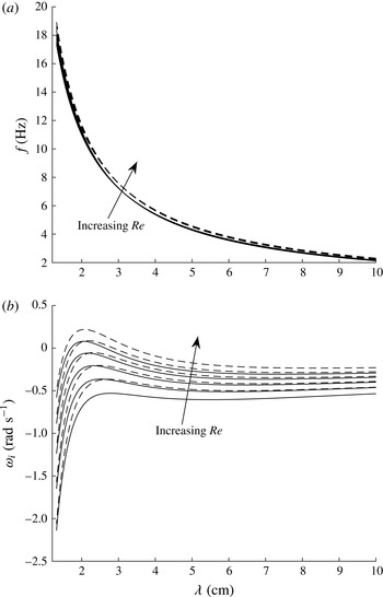
Figure 11. Numerically computed (a) wave frequency and (b) growth rate in Case 1 with the gas $Re$ being increased by $(0,10,20,30,40)\,\%$ with $h_{L}=0.44~\text{cm}$ (——) and $h_{L}=0.48~\text{cm}$ (– – –). (Note that in (a), all of the curves for a given liquid depth (but different values of $Re$ ) are graphically indistinguishable from each other.)

In each case, the gas Reynolds number is satisfied by definition of the solution strategy, while the experimentally reported values of the liquid flow conditions are reproduced to within a reasonable level of accuracy. This discrepancy is attributed to a few features. First, it is unlikely that the experimental apparatus is able to achieve a perfect fully developed turbulent profile in the entrance region of the channel. Therefore, some small deviation from the modelled velocity profile is expected. Second, the experimental wave probe measurements exhibit oscillations in the mean liquid depth. Such variations can perturb the velocity profile and result in a small departure from the model profile. However, this level of accuracy shown in table 4 will be shown to be sufficient, and present with accurate comparisons against the experimental measurements. Additionally, a turbulent linear stability analysis of the experimental flow conditions listed in table 4 is found to be marginally stable (as shown in figures 11 b, 14 b and 17 b). This is not surprising, in light of the reasons listed earlier in this paragraph. In order to examine the interfacial stability, while acknowledging the effect of these weak inconsistencies between the experimental and modelled flow conditions, a sensitivity analysis is carried out to show the robustness of our reported findings. For each test, the flow conditions based on table 4 are used along with flow conditions based on slightly perturbed gas Reynolds numbers. An additional set of tests are carried out using a perturbed liquid depth. Such a study shows the consistency of our predicted behaviour and validates that our conclusions are true within the neighbourhood of the experimental parameter space.

6.2 Method for resonance identification

Using the modelled velocity profile described in § 6.1, a turbulent Orr–Sommerfeld analysis is carried out for the determination of the interfacial wave frequency and growth rates. Using this calculated spectrum, a grid search is conducted to identify all possible modes that satisfy the subharmonic and triad resonance conditions, stated as $\{k_{2}-k_{1}/2=0,\unicode[STIX]{x1D714}_{2}-\unicode[STIX]{x1D714}_{1}/2=\unicode[STIX]{x1D70E}_{sub}\}$ and $\{k_{2}-k_{1}-k_{3}=0,\unicode[STIX]{x1D714}_{2}-\unicode[STIX]{x1D714}_{1}-\unicode[STIX]{x1D714}_{3}=\unicode[STIX]{x1D70E}_{triad}\}$ , respectively. As in § 2.2, $\unicode[STIX]{x1D70E}_{sub/triad}$ denotes the resonance detuning parameter. Values of this parameter closest to zero indicate the strongest resonant modes in the spectrum.

Due to the large volume of frequencies associated with each wavenumber in the discrete Orr–Sommerfeld spectrum, a large number of possible resonant combinations may exist. However, many of these modes may present with strong linear decay rates which are $O(-10^{3})$ . Given these high damping rates, it is not expected that these modes would play a significant role in energy transfer and result in long-wave growth. Therefore, a filter is imposed to the resonance analysis, which only allows modes where $\unicode[STIX]{x1D714}_{i}>-0.2$ be considered. Sensitivity studies are carried out to demonstrate that this value of $\min \{\unicode[STIX]{x1D714}_{i}\}$ does not alter the robustness of the resulting trends.

6.3 Strong subharmonic resonance case

Case 1 from table 4 corresponds to the experimental results shown in Jurman et al. (Reference Jurman, Deutsch and McCready1992, figure 7). The experimental wave spectra show that, during the initial phase of evolution, a fundamental mode with a frequency of approximately 7–9 Hz forms due to a linear instability. Wave probe measurements of the wave speed provide an estimate of 2.3 cm for the wavelength of this fundamental mode. As the wave propagates down the length of the channel, the wave spectrum evolves, adjusting the fundamental wave frequency to be centred at $f_{fund}\approx 9{-}10$ Hz. Eventually, as the waves become steeper, the interface develops a strong subharmonic component with a frequency that is approximately half the frequency of the unstable fundamental mode $(f_{sub}=1/2f_{fund})$ .

In order to demonstrate that this experimentally observed spectral evolution is due to the coupled instability–resonance mechanism, it is necessary to show that: (i) the fundamental mode is linearly unstable while the subharmonic is linearly stable (or damped), (ii) the frequencies of the unstable modes are consistent with the experimental measurements, and (iii) the unstable fundamental and the subharmonic frequencies and wavelengths (wavenumbers) satisfy the subharmonic resonance conditions.

Table 5. Peak growth rate ( $\unicode[STIX]{x1D714}_{I,max}$ ) and corresponding wavelength ( $\unicode[STIX]{x1D706}(\unicode[STIX]{x1D714}_{I,max})$ ) and frequency ( $f(\unicode[STIX]{x1D714}_{I,max})$ ) as a function of gas Reynolds number perturbation ( $\unicode[STIX]{x0394}Re$ ) and liquid equilibrium depth ( $h_{L}$ ) in Case 1. $\unicode[STIX]{x0394}\{Re\}=Re_{G,mean}^{(E)}(1+(\unicode[STIX]{x1D6E5}/100))$ . The fifth column represents the frequency band of linearly unstable waves (with a line indicating a stable spectrum). The sixth column represents the wavelength ( $\unicode[STIX]{x1D706}$ ) and frequency ( $f$ ) of the unstable fundamental mode corresponding to the strongest subharmonic resonance (shown in figure 12 for which $\unicode[STIX]{x1D70E}_{min}\equiv \min |\unicode[STIX]{x1D70E}|$ ). The last column represents the magnitude of the subharmonic resonance detuning parameter ( $\unicode[STIX]{x1D70E}$ ) for the fundamental mode of peak growth rate. ( $h_{L}$ , $\unicode[STIX]{x1D706}$ : cm; $f$ : Hz; $\unicode[STIX]{x1D714}_{I,max}$ , $\unicode[STIX]{x1D70E}$ : $\text{rad}~\text{s}^{-1}$ .)

Figures 11(a) and 11(b) show respectively the wave frequency and growth-rate spectra predicted by the turbulent Orr–Sommerfeld stability analysis with the flow conditions of Case 1. To show the sensitivity of these curves to the flow conditions, the results at two liquid depths of $h_{L}=0.44~\text{cm}$ and $0.48~\text{cm}$ with five perturbed gas Reynolds numbers (for each $h_{L}$ ), $Re=Re_{G,mean}^{(E)}(1+(j/100))$ , with $j=0,10,20,30,40$ , are displayed and compared. The frequency exhibits only a weak dependence on gas Reynolds number $Re$ and $h_{L}$ , while the growth rate ( $\unicode[STIX]{x1D714}_{I}$ ) shows a regularly increasing trend with $Re$ and $h_{L}$ . As $Re$ is increased, the wavelength corresponding to the peak growth rate, $\unicode[STIX]{x1D706}(\unicode[STIX]{x1D714}_{I,max})$ , experiences a small, but consistent, downshift to smaller values. For clarity, $\unicode[STIX]{x1D714}_{I,max}$ , $\unicode[STIX]{x1D706}(\unicode[STIX]{x1D714}_{I,max})$ and $f(\unicode[STIX]{x1D714}_{I,max})$ for each of these perturbed cases are documented in table 5. In the experimental measurement, the frequency of the initial unstable disturbance is centred around 7–9 Hz, and drifts towards 9–10 Hz with increasing fetch. The frequencies of unstable waves predicted by linear theory are in good agreement with those measurements. The range of $\unicode[STIX]{x1D706}(\unicode[STIX]{x1D714}_{I,max})$ is within $O(10\,\%)$ of the experimentally measured value.

The series of growth-rate curves, shown in figure 11(b), demonstrate that, for a sufficiently large perturbation, only a small band of wavelengths centred around the fundamental mode become linearly unstable. For small fetch, the experiments indicate that there is no wave growth near the subharmonic frequency. The theoretical spectrum is consistent with this observation, and shows that in the vicinity of subharmonic mode, denoted as $f_{sub}=1/2f_{fund},\unicode[STIX]{x1D706}_{sub}=2\unicode[STIX]{x1D706}_{fund}$ , all of the modes are linearly damped. Therefore, any observed growth of the subharmonic mode should not be due to the Orr–Sommerfeld instability, and is expected to be attributed to the nonlinearity of the flow.

Figure 12. Computed value of $\unicode[STIX]{x1D70E}=|\unicode[STIX]{x1D714}_{2}-\unicode[STIX]{x1D714}_{1}/2|$ for Case 1 from table 4 with gas $Re$ being increased by 0 % (○), 10 % (♢), 20 % (*), 30 % (▫), and 40 % (⨯) for (a) $h_{L}=0.44~\text{cm}$ and (b) $h_{L}=0.48~\text{cm}$ .

Figure 12 shows the magnitude of the subharmonic resonance detuning parameter as a function of fundamental wave frequency, $\unicode[STIX]{x1D70E}(f)$ , for the unperturbed liquid depth ( $h_{L}=0.44~\text{cm}$ ) and perturbed depth ( $h_{L}=0.48~\text{cm}$ ). (Note that each symbol shown in figure 12 denotes a single subharmonic resonant pair. There is no requirement for the $\unicode[STIX]{x1D70E}(f)$ curves to be continuous, and isolated resonant pairs are permitted to exist.) For both liquid depths, when $Re$ is unperturbed, there are no strong subharmonic resonances in the spectrum, since $\min \{\unicode[STIX]{x1D70E}\}=O(0.07{-}0.1)$ . However, as $Re$ is increased, strong subharmonic resonances are formed. For a 40 % perturbation of $Re$ at $h_{L}=0.44~\text{cm}$ , a strong subharmonic resonance is identified with $|\unicode[STIX]{x1D70E}|\approx 0$ at $f(\unicode[STIX]{x1D70E}\approx 0)=8.58~\text{Hz}$ . Analogously, for $h_{L}=0.48~\text{cm}$ , strong resonances are identified at $f(\unicode[STIX]{x1D70E}\approx 0)=9.76~\text{Hz}$ and 11.38 Hz for 30 % and 40 % perturbations of $Re$ , respectively. Significantly, the fundamental wave modes at these $f(\unicode[STIX]{x1D70E}\approx 0)$ values under the associated flow conditions are linearly unstable, since these $f(\unicode[STIX]{x1D70E}\approx 0)$ values fall in the bands of unstable wave frequencies, as shown in table 5. Together, these show the existence of the coupled instability–resonance mechanism in a laboratory setting, which can cause the growth of the linearly stable subharmonic mode through energy transfer from the linearly unstable fundamental mode. Moreover, the shape of these $\unicode[STIX]{x1D70E}(f)$ curves in the vicinity of $\unicode[STIX]{x1D70E}\approx 0$ indicates that this region of strong resonance is narrow banded, with only a small frequency range presenting with $|\unicode[STIX]{x1D70E}|\leqslant O(10^{-2})$ . This is consistent with the experimental observation that only a narrow band of frequencies centred around $f_{fund}$ and $f_{sub}$ achieves significant wave growth in the channel. We note that a second set of subharmonic resonances in the lower frequency range, such as those of $f\sim 3.7~\text{Hz}$ in figure 12(a) and $f\sim 3.4~\text{Hz}$ in figure 12(b), are irrelevant, since the associated fundamental modes are predicted to be linearly stable/damped.

Figure 12 shows that the increase in $Re$ and $h_{L}$ shifts $f(\unicode[STIX]{x1D70E}\approx 0)$ to higher wave frequencies (and smaller wavelengths). Table 5 lists the frequency $f(\unicode[STIX]{x1D70E}\approx 0)$ and the corresponding wavelength $\unicode[STIX]{x1D706}(\unicode[STIX]{x1D70E}\approx 0)$ under the perturbed flow conditions. It is seen from table 5 that, as $Re$ is increased, both $\unicode[STIX]{x1D706}(\unicode[STIX]{x1D714}_{I,max})$ and $\unicode[STIX]{x1D706}(\unicode[STIX]{x1D70E}\approx 0)$ decrease (while the corresponding wave frequencies increase). As the perturbation increases and finally destabilizes the interface (causing $\max \{\unicode[STIX]{x1D714}_{I}\}>0$ ), $\unicode[STIX]{x1D706}(\unicode[STIX]{x1D714}_{I,max})$ and $\unicode[STIX]{x1D706}(\unicode[STIX]{x1D70E}\approx 0)$ quickly approach each other, indicating the presence of a strong coupled instability–resonance process. For the unperturbed liquid depth case ( $h_{L}=0.44~\text{cm}$ ), the interface becomes unstable with a 40 % increase in $Re$ , at which the difference between $\unicode[STIX]{x1D706}(\unicode[STIX]{x1D714}_{I,max})$ and $\unicode[STIX]{x1D706}(\unicode[STIX]{x1D70E}\approx 0)$ is $O(20\,\%)$ . For the perturbed liquid depth case ( $h_{L}=0.48~\text{cm}$ ), the interface becomes unstable with 30–40 % perturbations of $Re$ , the resulting deviation between $\unicode[STIX]{x1D706}(\unicode[STIX]{x1D714}_{I,max})$ and $\unicode[STIX]{x1D706}(\unicode[STIX]{x1D70E}\approx 0)$ is $O(7\,\%)$ and $O(2\,\%)$ , respectively. This trend indicates that the effects of the coupled instability–resonance mechanism on the growth of linearly stable subharmonic waves become stronger as $Re$ and $h_{L}$ are increased. This is also reflected by the value of $|\unicode[STIX]{x1D70E}|$ for the fundamental mode of peak growth rate, which is closer to zero as $Re$ and $h_{L}$ are increased, as shown in table 5.

Figure 13. Computed value of $\unicode[STIX]{x1D70E}_{triad}=|\unicode[STIX]{x1D714}_{1}-\unicode[STIX]{x1D714}_{2}-\unicode[STIX]{x1D714}_{3}|$ for Case 1 from table 4 with a 40 % perturbation of $Re$ and $h_{L}=0.44~\text{cm}$ . Shown is $(k_{1},k_{2})$ -space with $k_{1}>k_{2}$ , with the space reduced to include only linearly unstable $k_{1}$ or $k_{2}$ modes.

Figure 14. Numerically computed (a) wave frequency and (b) growth rate corresponding to Case 2 with gas $Re$ being increased by $(0,5,10,15,20)\,\%$ with $h_{L}=0.36~\text{cm}$ (——) and $h_{L}=0.38~\text{cm}$ (– – –). (Note that in (a), all of the curves for a given liquid depth but different values of $Re$ are graphically indistinguishable from each other.)

The analysis for subharmonic resonant interactions can be extended to account for triad wave interactions that satisfy the conditions $k_{1}-k_{2}-k_{3}=0$ and $\unicode[STIX]{x1D714}_{1}-\unicode[STIX]{x1D714}_{2}-\unicode[STIX]{x1D714}_{3}=\unicode[STIX]{x1D70E}_{triad}$ . Due to the additional wavenumber component in this analysis, the resonant detuning results across the entire perturbed $Re$ range cannot be collapsed onto one plot. Therefore, only a representative case is shown. Figure 13 shows the variation of the minimum $\unicode[STIX]{x1D70E}_{triad}$ across the $(k_{1},k_{2})$ -space (for $k_{1}>k_{2}$ ). Since our interest is in the combined instability–resonance mechanism, figure 13 reduces $(k_{1},k_{2})$ -space to only those wavenumbers for which one or both of the $(k_{1},k_{2})$ modes are linearly unstable. The horizontal and vertical black lines contain the linearly unstable wavenumbers, while the dashed line indicates the wavenumber corresponding to the peak growth rate. The strongest resonances are found to be in the vicinity of $k_{1}\approx 2.5~\text{cm}^{-1}$ (consistent with the unstable mode identified from the experiments). Along this $k_{1}$ wavenumber, $\unicode[STIX]{x1D70E}_{triad}$ is near its minimum at approximately $k_{2}\approx k_{1}/2$ , verifying the presence of strong subharmonic resonance. By accounting for triad resonances, it becomes apparent that this band of $k_{2}$ wavenumbers centred around $k_{1}/2$ works to strengthen the resonant energy transfer to the subharmonic mode, and explains the broadening of the 5 Hz spectral peak observed in the original measurements Jurman et al. (Reference Jurman, Deutsch and McCready1992, figure 7). Additionally, following the diagonal along $k_{1}\simeq k_{2}$ , another band of strong resonances appear, for which $k_{3}=k_{2}-k_{1}\rightarrow 0$ . The value of $\unicode[STIX]{x1D70E}_{triad}$ is not as small as in the subharmonic region, but explains the eventual formation of the low-frequency peak ${\sim}O(1)~\text{Hz}$ shown in the experimental measurement.

6.4 Weaker subharmonic resonance case

This section examines Case 2 from table 4, which corresponds to the experimental results shown in Jurman et al. (Reference Jurman, Deutsch and McCready1992, figure 8). This trial is selected to demonstrate the impact of a larger value of the detuning parameter on the spectral evolution. The wave spectra for this experiment present with an initial instability, with unstable modes distributed between approximately 7–13 Hz centred around ${\sim}O(9)~\text{Hz}$ . As the waves propagate down the channel, the wave spectrum evolves and develops a small subharmonic peak centred around 4–5 Hz; however, the amount of energy transfer is significantly smaller than that in Case 1. It will be shown that these flow conditions still satisfy those of the coupled instability–resonance mechanism, but are composed of weaker subharmonic resonances (indicated by larger values of $|\unicode[STIX]{x1D70E}|$ ). These weaker resonances lead to slower growth of the linearly stable subharmonic wave components.

Using these flow conditions reported in table 4, the turbulent Orr–Sommerfeld growth rate and frequency spectra are calculated, as shown in figure 14. As in the previous case, a sensitivity analysis is conducted, which generates additional spectral curves for perturbed Reynolds number, $Re=Re_{G,mean}^{(E)}(1+(j/100))$ , with $j=0,5,10,15,20$ , at the reported liquid depth of $h_{L}=0.36~\text{cm}$ and at slightly deeper liquid depth of $h_{L}=0.38~\text{cm}$ . The maximum growth rate and corresponding wavelength and frequency for each test are tabulated in table 6.

Table 6. Peak growth rate ( $\unicode[STIX]{x1D714}_{I,max}$ ) and corresponding wavelength ( $\unicode[STIX]{x1D706}(\unicode[STIX]{x1D714}_{I,max})$ ) and frequency ( $f(\unicode[STIX]{x1D714}_{I,max})$ ) as a function of gas Reynolds number perturbation ( $\unicode[STIX]{x0394}Re$ ) and liquid equilibrium depth ( $h_{L}$ ) in Case 2. $\unicode[STIX]{x0394}\{Re\}=Re_{G,mean}^{(E)}(1+(\unicode[STIX]{x1D6E5}/100))$ . The fifth column represents the frequency band of linearly unstable waves (with a line indicating a stable spectrum). The sixth column represents the wavelength $(\unicode[STIX]{x1D706})$ and frequency $(f)$ of the unstable fundamental mode corresponding to the strongest subharmonic resonance (shown in figure 15 for which $\unicode[STIX]{x1D70E}_{min}\equiv \min |\unicode[STIX]{x1D70E}|$ ). The last column indicates the magnitude of the subharmonic resonance detuning parameter ( $\unicode[STIX]{x1D70E}$ ) for the fundamental mode of peak growth rate. ( $h_{L}$ , $\unicode[STIX]{x1D706}$ : cm; $f$ : Hz; $\unicode[STIX]{x1D714}_{I,max}$ , $\unicode[STIX]{x1D70E}$ : $\text{rad}~\text{s}^{-1}$ .)

The frequency curves show a weak dependency on the $Re$ and $h_{L}$ perturbations, while the growth rate exhibits a stronger dependency. As $Re$ increases, the growth rate increases and the peak experiences a weak downshift to shorter wavelengths. As the spectrum becomes unstable, the bandwidth of unstable modes increases rapidly. Despite this large band of unstable modes, the majority have weak growth rates, with the strongest instabilities being concentrated among the shorter waves with $\unicode[STIX]{x1D706}\sim O(1.5{-}2)~\text{cm}$ . This increase in the bandwidth of the unstable wavelength is consistent with the experimental spectra.

The resonance identification scheme shows that there are a large number of wave modes that approximately satisfy the resonance condition, as is shown in figure 15. For both liquid depth cases, as $Re$ increases, a strong subharmonic resonance forms. Although $f(\unicode[STIX]{x1D70E}\approx 0)$ falls in the unstable band, it is well away from the peak growth, as indicated in table 6. Since the fundamental mode is marginally unstable (with a small growth rate), the resulting energy transfer due to the subharmonic resonance is weak. In each test the subharmonic detuning parameter associated with the peak growth wave mode is found to be $\unicode[STIX]{x1D70E}(f_{peak})=O(2)$ , indicating weak subharmonic resonances associated with wave modes near the peak growth. These together show that, in this case, the combined instability and subharmonic resonance mechanism plays a role, but with much weaker energy transfer rate than in Case 1, which is consistent with experimental observation.

Figure 15. Computed value of $\unicode[STIX]{x1D70E}=|\unicode[STIX]{x1D714}_{2}-\unicode[STIX]{x1D714}_{1}/2|$ for Case 2 from table 4 with the Reynolds number being increased by 0 % (○), 5 % (♢), 10 % (*), 15 % (▫), and 20 % (⨯) for (a) $h_{L}=0.36~\text{cm}$ and (b) $h_{L}=0.38~\text{cm}$ .

As in the previous case, the analysis for subharmonic resonance can be extended to account for the role of triad resonance on the spectral evolution. Figure 16 shows the minimum value of the resonant detuning parameter across the linearly unstable portion of the $(k_{1},k_{2})$ -plane (for $k_{1}>k_{2}$ ). As in the previous case, along $k_{1}\approx 2.25~\text{cm}^{-1}$ there is a band of wavenumber $k_{2}\in [0.5,2]~\text{cm}^{-1}$ which all form weak triad resonance and strengthen the previously identified weak subharmonic resonance. Based on the magnitude of the detuning parameter, these resonances are significantly weaker than those described in Case 1. The strongest unstable triad resonances occur for $k_{1}\simeq k_{2}$ , which allows for some of the unstable energy to be passed to a long-wavelength (difference wavenumber) component, allowing energy to accumulate at the low-frequency range of the spectrum. This prediction is consistent with the reported experimental findings.

Figure 16. Computed value of $\unicode[STIX]{x1D70E}_{triad}=|\unicode[STIX]{x1D714}_{1}-\unicode[STIX]{x1D714}_{2}-\unicode[STIX]{x1D714}_{3}|$ for Case 2 from table 4 with a 15 % perturbation of $Re$ and $h_{L}=0.36~\text{cm}$ . The shown is $(k_{1},k_{2})$ -space with $k_{1}>k_{2}$ , with the space reduced to include only linearly unstable $k_{1}$ or $k_{2}$ modes.

6.5 Non-resonant case

This final example considers Case 3 from table 4, which corresponds to the test results shown in Jurman et al. (Reference Jurman, Deutsch and McCready1992, figure 6). This trial is selected to demonstrate a limiting case for which the value of the detuning parameter is so large that there is effectively no resonant energy transfer or subharmonic formation.

The wave spectrum for this experiment shows a strong initial instability that is distributed between approximately 7–13 Hz and is centred around ${\sim}10~\text{Hz}$ . As the disturbance propagates down the length of the channel, the interface rapidly grows and then becomes nonlinearly bounded. The bandwidth of the unstable modes remains nearly constant throughout the whole experiment, with only a weak second harmonic developing at approximately 20 Hz. Due to the regularity of this behaviour, this 20 Hz peak is associated the second-order locked-wave component. Using the resonance analysis, it is shown that there are no strong resonant interactions in the spectrum which are simultaneously coupled to the instability. This observation is consistent with the experimental findings, and demonstrates that the proposed coupled instability–resonance mechanism is not strong in this case.

Figure 17. Numerically computed (a) wave frequency and (b) growth rate corresponding to Case 3 with the Reynolds numbers being increased by $(0,5,10,15,20)\,\%$ for $h_{L}=0.55~\text{cm}$ (——) and $h_{L}=0.59~\text{cm}$ (- - -). Note that in (a), all of the curves for a given liquid depth are graphically indistinguishable from each other.

The turbulent Orr–Sommerfeld spectrum is calculated, using the flow conditions reported in table 4 (and the same type of Reynolds number/liquid depth perturbation method used in the previous sections), and are presented in figure 17. As in the previous two cases, the wave frequency shows only a weak dependence on the Reynolds number and liquid depth, while the growth rate exhibits a much clearer dependency. The peak growth rate and corresponding frequency and wavelength are reported in table 7.

Table 7. Peak growth rate $(\unicode[STIX]{x1D714}_{I,max})$ and corresponding wavelength $(\unicode[STIX]{x1D706}(\unicode[STIX]{x1D714}_{I,max}))$ and frequency as a function of gas Reynolds number perturbation $(\unicode[STIX]{x0394}Re)$ and liquid equilibrium depth $(h_{L})$ in Case 3. $\unicode[STIX]{x0394}\{Re\}=Re_{G,mean}^{(E)}(1+(\unicode[STIX]{x1D6E5}/100))$ . The fifth column represents the frequency band of linearly unstable waves (with a line indicating a stable spectrum). The sixth column represents the wavelength $(\unicode[STIX]{x1D706})$ and frequency $(f)$ of the unstable fundamental mode corresponding to the strongest subharmonic resonance (shown in figure 18 for which $\unicode[STIX]{x1D70E}_{min}\equiv \min |\unicode[STIX]{x1D70E}|$ ). The last column indicates the magnitude of the subharmonic resonance detuning parameter ( $\unicode[STIX]{x1D70E}$ ) for the fundamental mode of peak growth rate. ( $h_{L}$ , $\unicode[STIX]{x1D706}$ : cm; $f$ : Hz; $\unicode[STIX]{x1D714}_{I,max}$ , $\unicode[STIX]{x1D70E}$ : $\text{rad}~\text{s}^{-1}$ .)

It is observed, for both liquid depth trials, that once the flow becomes unstable (with a 20 % perturbation of $Re$ ), the frequency of the peak growth rate is found to be consistent with the centre of the unstable band of frequencies reported by the experiment.

The results of the subharmonic resonance analysis are shown in figure 18. For the $h_{L}=0.55~\text{cm}$ trial, a number of strong subharmonic resonances are observed. When $Re$ is fixed at the experimental value, a subharmonic resonance is observed around $f(\unicode[STIX]{x1D70E}\approx 0)=7~\text{Hz}$ . However, table 7 shows that this flow is strongly damped. As $Re$ increases, $f(\unicode[STIX]{x1D70E}\approx 0)$ moves to higher wave frequencies. Once the interface transitions and becomes unstable, $f(\unicode[STIX]{x1D70E}\approx 0)$ has moved up to approximately 17 Hz and is well away from the band of unstable frequencies. Over the frequency band of unstable waves, the subharmonic detuning parameter $|\unicode[STIX]{x1D70E}|$ is determined to be $O(1)$ or larger, as shown in table 7. With such large values of the detuning parameter, the resulting energy transfer would be so inefficient that it is unlikely to register on the resulting wave spectrum. This finding is consistent with the experimental observations.

Figure 18. Computed value of $\unicode[STIX]{x1D70E}=|\unicode[STIX]{x1D714}_{2}-\unicode[STIX]{x1D714}_{1}/2|$ for Case 3 from table 4 with the Reynolds number being increased by 0 % (○), 5 % (♢), 10 % (*), 15 % (▫), and 20 % (⨯) for (a) $h_{L}=0.55~\text{cm}$ and (b) $h_{L}=0.59~\text{cm}$ .

Figure 19 shows that over the linearly unstable portion of the $(k_{1},k_{2})$ -plane, the resonance detuning parameter is ${\sim}O(1)$ or larger, indicating very weak triad interactions. Figure 19 shows that, within the bandwidth of linearly unstable modes, the only regions that contain strong triad resonances are $k_{1}\simeq k_{2}$ or $k_{2}\approx 0$ . The experimental measurement supports these theoretical predictions, and shows only the unstable waves achieve a significant wave height and a small spectral peak at the low end of the spectrum near $f\sim O(1)$ Hz.

Figure 19. Computed value of $\unicode[STIX]{x1D70E}_{triad}=|\unicode[STIX]{x1D714}_{1}-\unicode[STIX]{x1D714}_{2}-\unicode[STIX]{x1D714}_{3}|$ for Case 3 from table 4 with a 20 % perturbation of $Re$ and $h_{L}=0.55~\text{cm}$ . The shown is $(k_{1},k_{2})$ -space with $k_{1}>k_{2}$ , with the space reduced to include only linearly unstable $k_{1}$ or $k_{2}$ modes.

In §§ 6.3–6.5, three experimental cases are examined which present with distinct nonlinear spectral behaviours. In each trial, given only the mean operational flow conditions, a linear stability analysis coupled with a resonance search algorithm is able to identify the presence of a possible coupled instability–resonance mechanism. In each case, the theoretical predictions are in agreement with the frequency of the wave spectrum peak and location of any possible nonlinear subharmonics. Furthermore, parameter sensitivity trials demonstrate that this behaviour is not coincidental, but is clearly a solution valid in the neighbourhood of the experimental parameter space. This agreement between the theory and experiments strongly supports the existence of a coupled instability–resonance mechanism, and demonstrates the ability of this phenomenon to rapidly transfer energy from linearly unstable short waves to linearly stable (or damped) long waves.