


1 Introduction
Many complex fluids used in industrial applications exhibit yield stress behaviour, e.g. polymers, colloidal suspensions, foams, cement slurries, paints, muds, etc. (see Coussot Reference Coussot2005). Flows of these fluids are actively studied from theoretical, rheological and experimental perspectives (e.g. Balmforth, Frigaard & Ovarlez Reference Balmforth, Frigaard and Ovarlez2014; Coussot Reference Coussot2014). This paper addresses the non-inertial flow of single-phase yield stress fluids along uneven/rough-walled (two-dimensional) channels, e.g. approximating a fracture; see figure 1(a). Our paper has two main objectives. First, we wish to re-examine the usual approaches to providing a (nonlinear) Darcy-type flow law, and to show that such approaches may contain serious quantitative errors when yield stress fluid flows are considered, due to self-selection of the flowing region. Second, we aim to explore the details of the flow as the limiting pressure gradient is approached, showing that determination of the critical pressure gradient (or yield stress) for flow is non-trivial, but also tractable in some situations. In satisfying these objectives we also shed light on other complex features of yield stress fluid flows through these geometries.
Non-inertial flows of Newtonian fluids are governed by the Stokes equations. Porous media and fractures cover a wide range of extremely complex geometries, but the linearity inherent in the Newtonian constitutive law means that the flow rate and pressure gradient are linearly related, as captured in Darcy’s law and observed experimentally. Mathematical study of Darcy-type flows, the development of closure models for permeability and the application to groundwater hydrology were all well advanced by the 1950s, as was an understanding of many limitations of Darcy’s law, e.g. inertial flows; see, e.g., Scheidegger (Reference Scheidegger1957). A general model for non-Darcy effects was proposed by Christianovich (Reference Christianovich1940), largely to extend mathematical analysis to such flows. Here, we are concerned with non-Darcy effects that arise due to the non-Newtonian character of the fluid.
The original motivation for much of this work stems from oil recovery. Different non-Newtonian effects were of primary interest in different world regions. The excellent review of Savins (Reference Savins1969), for example, covers shear-thinning and viscoelastic effects, as these were the additives being used for enhanced recovery in North America at the time, but does not mention yield stress effects. On the other hand, in the former USSR, heavy oils exhibiting viscoplastic behaviour were being extracted, and consequently the study of such fluids in porous media settings evolved there. Fibre-bundle or capillary-tube models of yield stress fluids flowing through a porous medium naturally lead to a limiting pressure gradient (LPG) which must be exceeded in order to flow. Thus, LPG generalizations of Darcy’s law into nonlinear filtration/seepage have been suggested and studied since the early 1960s, e.g. Sultanov (Reference Sultanov1960), Entov (Reference Entov1967). Entov (Reference Entov1967) attributes the first usage of LPG models for oil applications to Mirzadzhanzade (Reference Mirzadzhanzade1959). Mathematically analogous systems were in fact suggested earlier for water flowing through argillaceous rocks; i.e. the critical pressure acts on the pore space not the fluid. Early work concerning LPG flows is summarized in the text by Barenblatt, Entov & Ryzhik (Reference Barenblatt, Entov and Ryzhik1989) which contains further references.
Applications that involve flow along uneven channels are various. In hydraulic fracturing operations, some frac fluids used have a yield stress (designed in order to enhance proppant transport). At the end of hydraulic fracturing, the flowback phase attempts to clean the gelled fluids from the proppant-laden fracture. Sealants are routinely injected into brickwork to block the spread of moisture in old buildings (damp-proof courses). Cement injection into porous media is advocated as a means of sealing
 $\text{CO}_{2}$
storage reservoirs. Cement slurries and drilling fluids flow along uneven narrow eccentric annuli in the primary cementing process (see Nelson & Guillot Reference Nelson and Guillot2006). In the squeeze cementing process, oil and gas wells are repaired by injecting cements and other fine suspensions into thin cracks. Rock grouting represents another similar process; see El Tani (Reference El Tani2012). Injection of yield stress fluids has also been proposed as a potential method for porosimetry by Ambari et al. (Reference Ambari, Benhamou, Roux and Guyon1990).
$\text{CO}_{2}$
storage reservoirs. Cement slurries and drilling fluids flow along uneven narrow eccentric annuli in the primary cementing process (see Nelson & Guillot Reference Nelson and Guillot2006). In the squeeze cementing process, oil and gas wells are repaired by injecting cements and other fine suspensions into thin cracks. Rock grouting represents another similar process; see El Tani (Reference El Tani2012). Injection of yield stress fluids has also been proposed as a potential method for porosimetry by Ambari et al. (Reference Ambari, Benhamou, Roux and Guyon1990).
Due to the length scale of flows, geometric uncertainty and/or the need for industrial simplicity, it is often the case that nonlinear filtration/seepage approaches are preferred to (Navier–)Stokes formulations for practical flow computations. Determination of a closure relationship between the flow rate and the applied pressure, in porous or fractured materials, is consequently of interest. One approach is to consider flow through packed beds or porous structures, either experimentally (Park, Hawley & Blanks Reference Park, Hawley and Blanks1973; Al-Fariss & Pinder Reference Al-Fariss and Pinder1987; Chase & Dachavijit Reference Chase and Dachavijit2003, Reference Chase and Dachavijit2005; Clain Reference Clain2010; Chevalier et al. Reference Chevalier, Chevalier, Clain, Dupla, Canou, Rodts and Coussot2013a ) or numerically (Balhoff & Thompson Reference Balhoff and Thompson2004; Bleyer & Coussot Reference Bleyer and Coussot2014). The flow laws developed typically conform to the LPG type. This type of experiment can also be simulated using pore-throat or similar macro-scale models of the porous medium. In such models, a pore network or lattice is connected by capillary tubes along which one-dimensional (1D) flows (or similar closures) are assumed (see Roux & Herrmann Reference Roux and Herrmann1987; Sahimi Reference Sahimi1995; Balhoff & Thompson Reference Balhoff and Thompson2004; Chen, Rossen & Yortsos Reference Chen, Rossen and Yortsos2005; Sochi & Blunt Reference Sochi and Blunt2008; Balhoff et al. Reference Balhoff, Sanchez-Rivera, Kwok, Mehmani and Prodanović2012; Talon & Bauer Reference Talon and Bauer2013; Talon et al. Reference Talon, Auradou, Pessel and Hansen2013; Chevalier & Talon Reference Chevalier and Talon2015). Heterogeneity can be introduced into the network via local throat resistance or length, either systematically or stochastically. Since each flow path experiences different heterogeneous pore throats, their critical opening pressures are different. As a result, the disorder of the porous medium induces a hierarchy in the flow paths that open, leading to a non-trivial relationship between the flow rate and the applied pressure drop (see Talon et al. Reference Talon, Auradou, Pessel and Hansen2013; Chevalier & Talon Reference Chevalier and Talon2015).
Other approaches to deriving (LPG) closure flow laws are mostly classical. In the so-called ‘fibre-bundle model’ (e.g. Chen et al. Reference Chen, Rossen and Yortsos2005; de Castro et al. Reference de Castro, Omari, Ahmadi-Sénichault and Bruneau2014), the homogeneous porous medium is considered as a succession of parallel tubes, each with a uniform cross-sectional area. The flow law is easily derived in each throat and the critical pressure is known. The major drawback is, of course, that it neglects the influence of heterogeneity along each flow path. For two-dimensional (2D) fractures/fissures/channels the most classical approach is to assume a lubrication or Hele-Shaw approximation, e.g. Ge (Reference Ge1997), Drazer & Koplik (Reference Drazer and Koplik2000), Malevich, Mityushev & Adler (Reference Malevich, Mityushev and Adler2006); i.e. the mean flow is driven by a uniform pressure gradient along the varying gap. This approach has long been exploited in the modelling of laminar primary cementing flows, e.g. Bittleston, Ferguson & Frigaard (Reference Bittleston, Ferguson and Frigaard2002), Pelipenko & Frigaard (Reference Pelipenko and Frigaard2004). After some algebra involving the solution of the Buckingham–Reiner equation, the flow rate can be related to the local width of the gap (inducing heterogeneity). In a single rough channel, Talon, Auradou & Hansen (Reference Talon, Auradou and Hansen2014) show that the critical pressure is proportional to the harmonic mean of the gap width, and the flow–pressure relationship is related to a series of power means. In non-uniform Hele-Shaw geometries, the critical pressure is locally defined and the fluid flows preferentially (similarly to pore-throat network approaches). For example, in the eccentric annular cementing flows of Bittleston et al. (Reference Bittleston, Ferguson and Frigaard2002) and Pelipenko & Frigaard (Reference Pelipenko and Frigaard2004), the widest part of the annulus can flow while the narrowest part is stationary.
In this paper, we look at the effects of heterogeneity along a single channel (assumed to be 2D). We use accurate computations to solve the Stokes flow of a Bingham fluid flowing along complex fracture-like geometries and analyse the results to draw quantitative and qualitative conclusions useful for more general LPG-style closures. While the Hele-Shaw/lubrication approach (or indeed a fibre-bundle approach) can be straightforwardly applied to randomized varying gap widths, it has long been recognized that to do so may result in significant error where yield stress fluids are concerned. First of all, one faces the usual geometric restrictions of slow geometric variation which are likely to be invalid for many fractures. Second, the use of Hele-Shaw/lubrication scaling arguments needs careful attention (Walton & Bittleston Reference Walton and Bittleston1991; Balmforth & Craster Reference Balmforth and Craster1999; Putz, Frigaard & Martinez Reference Putz, Frigaard and Martinez2009), and the leading-order stress fields exhibit an
 $O(1)$
deviation from those of the naïve Hele-Shaw/lubrication approach. These errors arise from extensional stresses within the central plug, causing it to yield for modest heterogeneities (see Frigaard & Ryan Reference Frigaard and Ryan2004; Putz et al.
Reference Putz, Frigaard and Martinez2009).
$O(1)$
deviation from those of the naïve Hele-Shaw/lubrication approach. These errors arise from extensional stresses within the central plug, causing it to yield for modest heterogeneities (see Frigaard & Ryan Reference Frigaard and Ryan2004; Putz et al.
Reference Putz, Frigaard and Martinez2009).
Larger-amplitude heterogeneity leads to the emergence of so-called ‘fouling layers’ at the walls of the duct, in which residual fluid is held stationary by the yield stress. This geometric effect has been observed in various experimental and computational/analytical studies (de Souza Mendes et al.
Reference de Souza Mendes, Naccache, Varges and Marchesini2007; Chevalier et al.
Reference Chevalier, Rodts, Chateau, Boujlel, Maillard and Coussot2013b
; Roustaei & Frigaard Reference Roustaei and Frigaard2013; Bleyer & Coussot Reference Bleyer and Coussot2014; Roustaei, Gosselin & Frigaard Reference Roustaei, Gosselin and Frigaard2015). Roustaei & Frigaard (Reference Roustaei and Frigaard2013) demonstrate that as the heterogeneity amplitude increases at fixed yield stress, fouling occurs beyond a critical amplitude, and give an empirical prediction for the onset of fouling. Such predictions are, however, strongly dependent on the specific geometry; e.g. in the abrupt expansion of de Souza Mendes et al. (Reference de Souza Mendes, Naccache, Varges and Marchesini2007), fouling occurs first in the corners, whereas for the smooth geometries of Roustaei & Frigaard (Reference Roustaei and Frigaard2013), fouling is first found in the deepest part of the channel. The most important result, from the perspective of predicting flow-rate–pressure-drop relationships, is that fouling results in self-selection of an
 $O(1)$
variation of the flowing geometry (Roustaei et al.
Reference Roustaei, Gosselin and Frigaard2015), which should therefore have an
$O(1)$
variation of the flowing geometry (Roustaei et al.
Reference Roustaei, Gosselin and Frigaard2015), which should therefore have an
 $O(1)$
effect on such relationships. Such phenomena have not been systematically studied from the perspective of flow rate–pressure drop, as we do here.
$O(1)$
effect on such relationships. Such phenomena have not been systematically studied from the perspective of flow rate–pressure drop, as we do here.
Second, we have the objective of understanding and quantifying the flow onset problem; i.e. in a given section of an uneven fracture, what is the critical pressure drop at which the fluid begins to flow? Although having a porous media flow objective, the methods we use focus on solving Stokes equations. The fracture geometry defines the flow (uniquely for given physical parameters) and hence the flow onset or limiting pressure drop. However, the reverse is not true, as shown nicely by Balhoff & Thompson (Reference Balhoff and Thompson2004), i.e. the same limiting pressure drops are found for different geometries. For non-Newtonian fluids the geometry and rheology are closely coupled in determining a closure law. Use of multi-dimensional flow simulation is an essential tool for uncovering localized flow features which explain physical results that appear to be non-intuitive, e.g. as in Bleyer & Coussot (Reference Bleyer and Coussot2014).
The plan of the paper is as follows. In § 2, we present the model problem and fracture geometries that we consider in this paper, scale the corresponding equations, give an overview of the computational method and present example results. This is followed in § 3 by a systematic comparison of the flow-rate–pressure-drop relationships from the computations with those from a naïve lubrication approximation, including some methods to improve the approximations in the situation where fouling occurs. Section 4 focuses on analysis of the critical limit of zero flow, from both the mathematical and computational perspectives. This is largely focused on characterizing the limiting flows in simple fracture geometries, although insights are also gained from these results for more complicated and realistic fractures. The paper closes with a discussion of the main results and future directions.
2 Model set-up
Figure 1 shows the flow geometry and notation used in the current study. We assume a fracture of nominal minimal width
 $2\hat{D}$
, with walls located at
$2\hat{D}$
, with walls located at
 ${\hat{y}}=\pm [\hat{D}+{\hat{Y}}_{\pm }(\hat{x})]$
, where
${\hat{y}}=\pm [\hat{D}+{\hat{Y}}_{\pm }(\hat{x})]$
, where
 $0\leqslant {\hat{Y}}_{\pm }(\hat{x})\leqslant {\hat{H}}$
. Both walls and the flow are assumed to be periodic in
$0\leqslant {\hat{Y}}_{\pm }(\hat{x})\leqslant {\hat{H}}$
. Both walls and the flow are assumed to be periodic in
 $\hat{x}$
with period
$\hat{x}$
with period
 $\hat{L}$
. The periodic fracture cell is assumed to be filled with a yield stress fluid (assumed to be a Bingham fluid for simplicity), which is flowing non-inertially. As we wish to understand how Darcy-law-type behaviour is modified geometrically and rheologically, we are interested in the mapping from flow rate (mean velocity) to pressure drop (and vice versa).
$\hat{L}$
. The periodic fracture cell is assumed to be filled with a yield stress fluid (assumed to be a Bingham fluid for simplicity), which is flowing non-inertially. As we wish to understand how Darcy-law-type behaviour is modified geometrically and rheologically, we are interested in the mapping from flow rate (mean velocity) to pressure drop (and vice versa).

Figure 1. (a) Schematic of the 2D fracture showing the dimensional parameters; (b) schematic of the wavy-walled dimensionless geometry, with the lower wall shifted to the right by
 $\unicode[STIX]{x1D713}L$
.
$\unicode[STIX]{x1D713}L$
.
In a fracture of varying width the areal flow rate
 $\hat{Q}$
is constant and the pressure gradient varies along the flow direction. Therefore, an imposed flow formulation will be adopted. To make the Stokes equations dimensionless we use
$\hat{Q}$
is constant and the pressure gradient varies along the flow direction. Therefore, an imposed flow formulation will be adopted. To make the Stokes equations dimensionless we use
 $\hat{D}$
as the length scale. Let
$\hat{D}$
as the length scale. Let
 $\hat{U} _{0}$
denote the mean velocity along the fracture, defined at the minimum fracture width, i.e.
$\hat{U} _{0}$
denote the mean velocity along the fracture, defined at the minimum fracture width, i.e.
 $\hat{U} _{0}=\hat{Q}/2\hat{D}$
. We use
$\hat{U} _{0}=\hat{Q}/2\hat{D}$
. We use
 $\hat{U} _{0}$
to scale the velocity. The shear stresses are then scaled with
$\hat{U} _{0}$
to scale the velocity. The shear stresses are then scaled with
 $\hat{\unicode[STIX]{x1D707}}\hat{U} _{0}/\hat{D}$
, where
$\hat{\unicode[STIX]{x1D707}}\hat{U} _{0}/\hat{D}$
, where
 $\hat{\unicode[STIX]{x1D707}}$
is the plastic viscosity of the Bingham fluid. Any static pressure component is subtracted from the pressure, before also scaling with
$\hat{\unicode[STIX]{x1D707}}$
is the plastic viscosity of the Bingham fluid. Any static pressure component is subtracted from the pressure, before also scaling with
 $\hat{\unicode[STIX]{x1D707}}\hat{U} _{0}/\hat{D}$
. In the remainder of the paper, we consistently use the ‘hat’ symbol to denote variables that are dimensional, e.g.
$\hat{\unicode[STIX]{x1D707}}\hat{U} _{0}/\hat{D}$
. In the remainder of the paper, we consistently use the ‘hat’ symbol to denote variables that are dimensional, e.g.
 $\hat{x}$
, and dimensionless variables are denoted without a hat, e.g.
$\hat{x}$
, and dimensionless variables are denoted without a hat, e.g.
 $x$
. The dimensionless Stokes equations are
$x$
. The dimensionless Stokes equations are
 $$\begin{eqnarray}\displaystyle & \displaystyle 0=-\frac{\unicode[STIX]{x2202}p}{\unicode[STIX]{x2202}x}+\frac{\unicode[STIX]{x2202}}{\unicode[STIX]{x2202}x}\unicode[STIX]{x1D70F}_{xx}+\frac{\unicode[STIX]{x2202}}{\unicode[STIX]{x2202}y}\unicode[STIX]{x1D70F}_{xy}, & \displaystyle\end{eqnarray}$$
 $$\begin{eqnarray}\displaystyle & \displaystyle 0=-\frac{\unicode[STIX]{x2202}p}{\unicode[STIX]{x2202}y}+\frac{\unicode[STIX]{x2202}}{\unicode[STIX]{x2202}x}\unicode[STIX]{x1D70F}_{yx}+\frac{\unicode[STIX]{x2202}}{\unicode[STIX]{x2202}y}\unicode[STIX]{x1D70F}_{yy}, & \displaystyle\end{eqnarray}$$
 $$\begin{eqnarray}\displaystyle & \displaystyle 0=\frac{\unicode[STIX]{x2202}u}{\unicode[STIX]{x2202}x}+\frac{\unicode[STIX]{x2202}v}{\unicode[STIX]{x2202}y}, & \displaystyle\end{eqnarray}$$
where
 $\boldsymbol{u}=(u,v)$
is the velocity,
$\boldsymbol{u}=(u,v)$
is the velocity,
 $p$
is the modified pressure and
$p$
is the modified pressure and
 $\unicode[STIX]{x1D70F}_{ij}$
is the deviatoric stress tensor. The scaled constitutive laws are
$\unicode[STIX]{x1D70F}_{ij}$
is the deviatoric stress tensor. The scaled constitutive laws are
 $$\begin{eqnarray}\displaystyle & \displaystyle \unicode[STIX]{x1D70F}_{ij}=\left(1+\frac{B}{\dot{\unicode[STIX]{x1D6FE}}(\boldsymbol{u})}\right)\dot{\unicode[STIX]{x1D6FE}}_{ij}\Longleftrightarrow \unicode[STIX]{x1D749}>B, & \displaystyle\end{eqnarray}$$
 $$\begin{eqnarray}\displaystyle & \displaystyle \dot{\unicode[STIX]{x1D6FE}}_{ij}(\boldsymbol{u})=0\Longleftrightarrow \unicode[STIX]{x1D749}\leqslant B, & \displaystyle\end{eqnarray}$$
where
 $$\begin{eqnarray}\dot{\unicode[STIX]{x1D6FE}}_{ij}(\boldsymbol{u})=\frac{\unicode[STIX]{x2202}u_{i}}{\unicode[STIX]{x2202}x_{j}}+\frac{\unicode[STIX]{x2202}u_{j}}{\unicode[STIX]{x2202}x_{i}},\quad \boldsymbol{u}=(u,v)=(u_{1},u_{2}),\boldsymbol{x}=(x,y)=(x_{1},x_{2}),\end{eqnarray}$$
and
 $\dot{\unicode[STIX]{x1D6FE}}$
,
$\dot{\unicode[STIX]{x1D6FE}}$
,
 $\unicode[STIX]{x1D70F}$
are the norms of
$\unicode[STIX]{x1D70F}$
are the norms of
 $\dot{\unicode[STIX]{x1D6FE}}_{ij}$
,
$\dot{\unicode[STIX]{x1D6FE}}_{ij}$
,
 $\unicode[STIX]{x1D70F}_{ij}$
, defined as
$\unicode[STIX]{x1D70F}_{ij}$
, defined as
 $$\begin{eqnarray}\dot{\unicode[STIX]{x1D6FE}}=\sqrt{\frac{1}{2}\mathop{\sum }_{ij}\dot{\unicode[STIX]{x1D6FE}}_{ij}^{2}}\quad \text{and}\quad \unicode[STIX]{x1D70F}=\sqrt{\frac{1}{2}\mathop{\sum }_{ij}\unicode[STIX]{x1D70F}_{ij}^{2}}.\end{eqnarray}$$
A single dimensionless number appears above, the Bingham number,
 $B$
,
$B$
,
 $$\begin{eqnarray}B\equiv \frac{\hat{\unicode[STIX]{x1D70F}}_{Y}\hat{D}}{\hat{\unicode[STIX]{x1D707}}\hat{U} _{0}},\end{eqnarray}$$
which represents the competition between the yield stress
 $\hat{\unicode[STIX]{x1D70F}}_{Y}$
and the viscous stresses. Two other geometric groups characterize the fracture shape: the dimensionless length
$\hat{\unicode[STIX]{x1D70F}}_{Y}$
and the viscous stresses. Two other geometric groups characterize the fracture shape: the dimensionless length
 $L=\hat{L}/\hat{D}$
and the maximal out of gauge depth
$L=\hat{L}/\hat{D}$
and the maximal out of gauge depth
 $H={\hat{H}}/\hat{D}$
; see figure 1.
$H={\hat{H}}/\hat{D}$
; see figure 1.
No-slip conditions are satisfied at the upper and lower walls:
 $$\begin{eqnarray}\boldsymbol{u}=0,\text{ at }y=1+y_{+}(x)\text{ and }y=-1-y_{-}(x),\end{eqnarray}$$
where
 $y_{\pm }(x)={\hat{Y}}_{\pm }(\hat{x})/\hat{D}$
. At the ends of the fracture we impose periodicity:
$y_{\pm }(x)={\hat{Y}}_{\pm }(\hat{x})/\hat{D}$
. At the ends of the fracture we impose periodicity:
 $$\begin{eqnarray}\displaystyle & \left.\begin{array}{@{}c@{}}\displaystyle \boldsymbol{u}(-L/2,y)=\boldsymbol{u}(L/2,y),\quad \unicode[STIX]{x1D70F}_{ij}(-L/2,y)=\unicode[STIX]{x1D70F}_{ij}(L/2,y),\\ \displaystyle p(-L/2,y)=p(L/2,y)+\unicode[STIX]{x0394}p,\end{array}\right\} & \displaystyle\end{eqnarray}$$
 $$\begin{eqnarray}\displaystyle & \displaystyle 2=\int _{-1-y_{-}(x)}^{1+y_{+}(x)}u_{1}(x,y)\,\text{d}y. & \displaystyle\end{eqnarray}$$
Here,
 $\unicode[STIX]{x0394}p$
denotes the frictional pressure drop, which is part of the solution and is determined by satisfying the flow rate constraint (2.9).
$\unicode[STIX]{x0394}p$
denotes the frictional pressure drop, which is part of the solution and is determined by satisfying the flow rate constraint (2.9).
2.1 Fracture geometries
The dimensionless fracture wall shapes
 $y_{\pm }(x)$
satisfy the bounds
$y_{\pm }(x)$
satisfy the bounds
 $0\leqslant y_{\pm }(x)\leqslant H={\hat{H}}/\hat{D}$
. We consider two generic simplified fracture geometries (sinusoidal walls and triangular walls) and a more complex affine geometry. An example affine geometry is shown schematically in figure 1(a) and the sinusoidal wavy fracture in figure 1(b). The sinusoidal fracture widths are given by
$0\leqslant y_{\pm }(x)\leqslant H={\hat{H}}/\hat{D}$
. We consider two generic simplified fracture geometries (sinusoidal walls and triangular walls) and a more complex affine geometry. An example affine geometry is shown schematically in figure 1(a) and the sinusoidal wavy fracture in figure 1(b). The sinusoidal fracture widths are given by
 $$\begin{eqnarray}y_{+}(x)=\frac{H}{2}[1+\cos (2\unicode[STIX]{x03C0}x/L)],\quad y_{-}(x)=\frac{H}{2}[1+\cos (2\unicode[STIX]{x03C0}[x/L-\unicode[STIX]{x1D713}])],\end{eqnarray}$$
with
 $\unicode[STIX]{x1D713}\in [0,1]$
denoting a phase shift of the lower wall relative to the upper one, i.e. the lower wall is translated
$\unicode[STIX]{x1D713}\in [0,1]$
denoting a phase shift of the lower wall relative to the upper one, i.e. the lower wall is translated
 $\unicode[STIX]{x1D713}L$
to the right. The triangular geometry is defined analogously.
$\unicode[STIX]{x1D713}L$
to the right. The triangular geometry is defined analogously.
In many applications, it has been observed that fracture roughness may display self-affine correlations (Mandelbrot, Passoja & Paullay Reference Mandelbrot, Passoja and Paullay1984; Schmittbuhl, Gentier & Roux Reference Schmittbuhl, Gentier and Roux1993; Bouchaud Reference Bouchaud1997). A surface
 ${\hat{y}}(\hat{x})$
is self-affine if the probability to find the increment
${\hat{y}}(\hat{x})$
is self-affine if the probability to find the increment
 $\unicode[STIX]{x0394}{\hat{y}}$
after a distance
$\unicode[STIX]{x0394}{\hat{y}}$
after a distance
 $\unicode[STIX]{x0394}\hat{x}$
displays the scaling invariance
$\unicode[STIX]{x0394}\hat{x}$
displays the scaling invariance
 $$\begin{eqnarray}p(\unicode[STIX]{x0394}{\hat{y}},\unicode[STIX]{x0394}\hat{x})=\unicode[STIX]{x1D706}^{\unicode[STIX]{x1D701}}p(\unicode[STIX]{x1D706}^{\unicode[STIX]{x1D701}}\unicode[STIX]{x0394}{\hat{y}},\unicode[STIX]{x1D706}\unicode[STIX]{x0394}\hat{x}),\end{eqnarray}$$
where
 $\unicode[STIX]{x1D706}$
is any scaling factor and
$\unicode[STIX]{x1D706}$
is any scaling factor and
 $\unicode[STIX]{x1D701}$
is called the Hurst exponent. An important property of self-affine surfaces is that all of the moments scale with the length of measurement as
$\unicode[STIX]{x1D701}$
is called the Hurst exponent. An important property of self-affine surfaces is that all of the moments scale with the length of measurement as
 $$\begin{eqnarray}M_{n}(\hat{x})=(\langle |{\hat{y}}(\hat{x}+\unicode[STIX]{x0394}\hat{x})-{\hat{y}}(\hat{x})|^{n}\rangle )^{1/n}\propto |\unicode[STIX]{x0394}\hat{x}|^{\unicode[STIX]{x1D701}}.\end{eqnarray}$$
For the present paper, we have generated three types of fracture. In the first type, the two walls
 $y_{\pm }$
are independently generated with a Hurst exponent
$y_{\pm }$
are independently generated with a Hurst exponent
 $\unicode[STIX]{x1D701}=0.5$
using a Fourier transform method (see Sahimi Reference Sahimi1995; Talon, Auradou & Hansen Reference Talon, Auradou and Hansen2010). Both surfaces are scaled to have
$\unicode[STIX]{x1D701}=0.5$
using a Fourier transform method (see Sahimi Reference Sahimi1995; Talon, Auradou & Hansen Reference Talon, Auradou and Hansen2010). Both surfaces are scaled to have
 $\min y_{\pm }=0$
and
$\min y_{\pm }=0$
and
 $\max y_{\pm }=H$
. In the second type, we used
$\max y_{\pm }=H$
. In the second type, we used
 $y_{+}=y_{-}$
. In the third type, we used
$y_{+}=y_{-}$
. In the third type, we used
 $y_{+}=-y_{-}$
.
$y_{+}=-y_{-}$
.
2.2 Computational overview
Numerical solution of viscoplastic fluids poses a unique challenge, which is the singularity of the effective viscosity in the constitutive equation (2.4), where
 $\dot{\unicode[STIX]{x1D738}}\rightarrow 0$
(unyielded regions). Aside from such points, the Bingham fluid is simply a generalized Non-Newtonian fluid with an effective viscosity
$\dot{\unicode[STIX]{x1D738}}\rightarrow 0$
(unyielded regions). Aside from such points, the Bingham fluid is simply a generalized Non-Newtonian fluid with an effective viscosity
 $\unicode[STIX]{x1D707}=(1+B/\dot{\unicode[STIX]{x1D738}})$
. A common work around for the singular effective viscosity is to simply regularize the viscosity, introducing a small parameter
$\unicode[STIX]{x1D707}=(1+B/\dot{\unicode[STIX]{x1D738}})$
. A common work around for the singular effective viscosity is to simply regularize the viscosity, introducing a small parameter
 $\unicode[STIX]{x1D716}\ll 1$
, such that the effective viscosity scales like
$\unicode[STIX]{x1D716}\ll 1$
, such that the effective viscosity scales like
 $\unicode[STIX]{x1D716}^{-1}$
as
$\unicode[STIX]{x1D716}^{-1}$
as
 $\dot{\unicode[STIX]{x1D738}}\rightarrow 0$
. Many such regularizations are possible. It can be shown that as
$\dot{\unicode[STIX]{x1D738}}\rightarrow 0$
. Many such regularizations are possible. It can be shown that as
 $\unicode[STIX]{x1D716}\rightarrow 0$
the velocity solution will converge to that of the exact Bingham fluid, but the stress field may not; see Frigaard & Nouar (Reference Frigaard and Nouar2005). Consequently, we may not infer the correct shape of the yield surface from
$\unicode[STIX]{x1D716}\rightarrow 0$
the velocity solution will converge to that of the exact Bingham fluid, but the stress field may not; see Frigaard & Nouar (Reference Frigaard and Nouar2005). Consequently, we may not infer the correct shape of the yield surface from
 $\unicode[STIX]{x1D70F}=B$
; e.g. Wang (Reference Wang1997).
$\unicode[STIX]{x1D70F}=B$
; e.g. Wang (Reference Wang1997).
Instead, we use the augmented Lagrangian (AL) method (Fortin & Glowinski Reference Fortin and Glowinski1983; Glowinski & Le Tallec Reference Glowinski and Le Tallec1989), which uses the proper variational formulation of the problem, as formulated, for example, by Duvaut & Lions (Reference Duvaut and Lions1976). The AL method introduces two new fields, the strain rate
 $\unicode[STIX]{x1D738}$
and stress
$\unicode[STIX]{x1D738}$
and stress
 $\unicode[STIX]{x1D64F}$
, in addition to the velocity and pressure
$\unicode[STIX]{x1D64F}$
, in addition to the velocity and pressure
 $(\boldsymbol{u},p)$
of the original problem. In this way, it relaxes the convex but non-differentiable velocity minimization problem to an associated saddle point problem. The saddle point problem is solved iteratively. Each iteration consists of three Uzawa split steps, to update
$(\boldsymbol{u},p)$
of the original problem. In this way, it relaxes the convex but non-differentiable velocity minimization problem to an associated saddle point problem. The saddle point problem is solved iteratively. Each iteration consists of three Uzawa split steps, to update
 $(\boldsymbol{u}^{n},p^{n})$
,
$(\boldsymbol{u}^{n},p^{n})$
,
 $\unicode[STIX]{x1D738}^{n}$
and
$\unicode[STIX]{x1D738}^{n}$
and
 $\unicode[STIX]{x1D64F}^{n}$
. These iterations are repeated until
$\unicode[STIX]{x1D64F}^{n}$
. These iterations are repeated until
 $\max \{|\unicode[STIX]{x1D738}^{n}-\dot{\unicode[STIX]{x1D738}}^{n}|_{L2},|\boldsymbol{u}^{n}-\boldsymbol{u}^{n-1}|\}\leqslant 10^{-6}$
is satisfied or a maximum number of iterations (here 10 000) is reached. The
$\max \{|\unicode[STIX]{x1D738}^{n}-\dot{\unicode[STIX]{x1D738}}^{n}|_{L2},|\boldsymbol{u}^{n}-\boldsymbol{u}^{n-1}|\}\leqslant 10^{-6}$
is satisfied or a maximum number of iterations (here 10 000) is reached. The
 $\unicode[STIX]{x1D738},\unicode[STIX]{x1D64F}$
fields of the AL method converge respectively to the strain rate and deviatoric stress tensors of the exact Bingham flow.
$\unicode[STIX]{x1D738},\unicode[STIX]{x1D64F}$
fields of the AL method converge respectively to the strain rate and deviatoric stress tensors of the exact Bingham flow.
The AL approach is effectively a fixed-point iteration and suffers from slow convergence. In recent years, a number of authors have been working on improving the convergence speed; e.g. de los Reyes & González Andrade (Reference de los Reyes and González Andrade2012), Treskatis, Moyers-Gonzalez & Price (Reference Treskatis, Moyers-Gonzalez and Price2015) and Saramito (Reference Saramito2016). While undoubtedly these approaches will come to fruition and common usage, familiarity with the AL approach and access to multiple CPUs has made the search for improved efficiency less urgent for the present study. We have implemented the AL method using the freely available FreeFEM++ finite element environment (Hecht Reference Hecht2012). Our algorithm is based on that of Saramito & Roquet (Reference Saramito and Roquet2001) with the addition of a flow rate constraint. To satisfy the inf–sup condition, Taylor–Hood
 $(P2{-}P1)$
elements are used for the velocity and pressure. Linear discontinuous elements
$(P2{-}P1)$
elements are used for the velocity and pressure. Linear discontinuous elements
 $P1_{d}$
are used for the
$P1_{d}$
are used for the
 $\unicode[STIX]{x1D738}$
and
$\unicode[STIX]{x1D738}$
and
 $\unicode[STIX]{x1D64F}$
fields, to follow compatibility conditions between the velocity space and the strain/stress spaces. Both the velocity and the pressure are implicitly solved and the system matrix is factorized once for all iterations. To improve the accuracy of the solution while keeping reasonable runtime, five cycles of the anisotropic mesh adaptation (Borouchaki et al.
Reference Borouchaki, George, Hecht, Laug and Saltel1997) are used.
$\unicode[STIX]{x1D64F}$
fields, to follow compatibility conditions between the velocity space and the strain/stress spaces. Both the velocity and the pressure are implicitly solved and the system matrix is factorized once for all iterations. To improve the accuracy of the solution while keeping reasonable runtime, five cycles of the anisotropic mesh adaptation (Borouchaki et al.
Reference Borouchaki, George, Hecht, Laug and Saltel1997) are used.
A typical computation presented below starts with a size of 8000–10 000 mesh points. A new mesh is generated based on a metric computed from the current solution. We use the dissipation field as the metric, which results in a finer mesh around the yield surface. After the fifth cycle, the mesh may contain up to 150 000 mesh points, and the yield surfaces can be clearly identified by a much finer local mesh. The underlying combination of discretization and algorithm is analysed in Saramito & Roquet (Reference Saramito and Roquet2001), with various benchmarks computed. More details on the numerical algorithm specific to channel flows are described in Roustaei & Frigaard (Reference Roustaei and Frigaard2013) and Roustaei et al. (Reference Roustaei, Gosselin and Frigaard2015) and are skipped here for conciseness.
2.3 Example results
We have computed over 2000 flows, covering a wide range of
 $H$
,
$H$
,
 $L$
and
$L$
and
 $B$
, for both triangular and wavy fracture profiles with different values of
$B$
, for both triangular and wavy fracture profiles with different values of
 $\unicode[STIX]{x1D713}$
. In addition, we have computed a smaller number of flows in affine fracture geometries. Before analysing specific features of the flow, we present some examples to illustrate qualitative features of our results.
$\unicode[STIX]{x1D713}$
. In addition, we have computed a smaller number of flows in affine fracture geometries. Before analysing specific features of the flow, we present some examples to illustrate qualitative features of our results.
Figure 2 shows results from a relatively modest fracture geometry and yield stress rheology (
 $H=1$
,
$H=1$
,
 $L=10$
,
$L=10$
,
 $B=2$
). Figure 2(a–d) shows the triangular and wavy profiles for
$B=2$
). Figure 2(a–d) shows the triangular and wavy profiles for
 $\unicode[STIX]{x1D713}=0$
(symmetric fracture). The flow is evidently symmetric about the centreline and the widest part of the fracture. Unyielded plug regions are found at the symmetry points in
$\unicode[STIX]{x1D713}=0$
(symmetric fracture). The flow is evidently symmetric about the centreline and the widest part of the fracture. Unyielded plug regions are found at the symmetry points in
 $x$
and close to the fracture centreline. There is very little difference, qualitatively or quantitatively, between triangular and wavy profiles. Figure 2(e,f) shows the wavy profile at
$x$
and close to the fracture centreline. There is very little difference, qualitatively or quantitatively, between triangular and wavy profiles. Figure 2(e,f) shows the wavy profile at
 $\unicode[STIX]{x1D713}=0.5$
, where the lower wall is out of phase with the upper wall. Here, the differences are quite significant. The velocity field appears to adapt smoothly to the wavy geometry, but no longer has the fastest fluid in the centre of each cross-section. Instead, the fastest travelling fluid moves at larger radius of curvature, while the plug regions are displaced into each bend. Due to symmetry effects, we observe a rather spectacular effect on the pressure field: the displaced central plug regions are joined by thin strands of unyielded fluid. It appears that the pressure is discontinuous across these strands, which is possible. It should be noted, however, that the traction vector, defined by the normal to these strands, is continuous.
$\unicode[STIX]{x1D713}=0.5$
, where the lower wall is out of phase with the upper wall. Here, the differences are quite significant. The velocity field appears to adapt smoothly to the wavy geometry, but no longer has the fastest fluid in the centre of each cross-section. Instead, the fastest travelling fluid moves at larger radius of curvature, while the plug regions are displaced into each bend. Due to symmetry effects, we observe a rather spectacular effect on the pressure field: the displaced central plug regions are joined by thin strands of unyielded fluid. It appears that the pressure is discontinuous across these strands, which is possible. It should be noted, however, that the traction vector, defined by the normal to these strands, is continuous.

Figure 2. Computed examples of speed
 $|\boldsymbol{u}|$
and streamlines (a,c,e), and pressure
$|\boldsymbol{u}|$
and streamlines (a,c,e), and pressure
 $p$
with (grey) unyielded plugs (b,d,f), at
$p$
with (grey) unyielded plugs (b,d,f), at
 $H=1$
,
$H=1$
,
 $L=10$
,
$L=10$
,
 $B=2$
. (a,b) Triangular fracture profile,
$B=2$
. (a,b) Triangular fracture profile,
 $\unicode[STIX]{x1D713}=0$
; (c,d) wavy fracture profile,
$\unicode[STIX]{x1D713}=0$
; (c,d) wavy fracture profile,
 $\unicode[STIX]{x1D713}=0$
; (e,f) wavy fracture profile,
$\unicode[STIX]{x1D713}=0$
; (e,f) wavy fracture profile,
 $\unicode[STIX]{x1D713}=0.5$
.
$\unicode[STIX]{x1D713}=0.5$
.
Figure 3 explores the effects of increasing the yield stress on the flow of figure 2 (
 $H=1$
,
$H=1$
,
 $L=10$
,
$L=10$
,
 $\unicode[STIX]{x1D713}=0$
). The flow, of course, remains symmetric and, since the flow rate is fixed, we only observe a relatively small change in the streamlines (figure 3
a,c,e) as
$\unicode[STIX]{x1D713}=0$
). The flow, of course, remains symmetric and, since the flow rate is fixed, we only observe a relatively small change in the streamlines (figure 3
a,c,e) as
 $B$
is increased. This, however, masks the changes that are occurring in the pressure and stress fields. Increasing
$B$
is increased. This, however, masks the changes that are occurring in the pressure and stress fields. Increasing
 $B$
results in a widening of the plugs in both narrow and wide parts of the fracture (figure 3
b,d,f). The magnitude of the pressure field also increases with
$B$
results in a widening of the plugs in both narrow and wide parts of the fracture (figure 3
b,d,f). The magnitude of the pressure field also increases with
 $B$
: the flow rate is fixed and the pressure gradient therefore needs to overcome the yield stress everywhere along the fracture to ensure flow (hence
$B$
: the flow rate is fixed and the pressure gradient therefore needs to overcome the yield stress everywhere along the fracture to ensure flow (hence
 $p/B$
is shown to aid comparison). For
$p/B$
is shown to aid comparison). For
 $B\approx 10$
we observe that a region of stationary fluid emerges at the upper and lower walls, in the deepest part of the fracture. We refer to this as a fouling layer. The fouling layer grows in size as
$B\approx 10$
we observe that a region of stationary fluid emerges at the upper and lower walls, in the deepest part of the fracture. We refer to this as a fouling layer. The fouling layer grows in size as
 $B$
increases. Growth of the fouling layer has effects on the pressure drop along the fracture and is an important part of the yield limit that is attained as
$B$
increases. Growth of the fouling layer has effects on the pressure drop along the fracture and is an important part of the yield limit that is attained as
 $B\rightarrow \infty$
, both of which are studied later; see § 4.
$B\rightarrow \infty$
, both of which are studied later; see § 4.

Figure 3. Computed examples of speed
 $|\boldsymbol{u}|$
and streamlines (a,c,e), and scaled pressure
$|\boldsymbol{u}|$
and streamlines (a,c,e), and scaled pressure
 $p/B$
with (grey) unyielded plugs (b,d,f), at
$p/B$
with (grey) unyielded plugs (b,d,f), at
 $H=1$
,
$H=1$
,
 $L=10$
,
$L=10$
,
 $\unicode[STIX]{x1D713}=0$
, wavy fracture profile; (a,b)
$\unicode[STIX]{x1D713}=0$
, wavy fracture profile; (a,b)
 $B=5$
, (c,d)
$B=5$
, (c,d)
 $B=10$
, (e,f)
$B=10$
, (e,f)
 $B=100$
.
$B=100$
.
Figure 4 explores the effects of increasing
 $H$
on the flow illustrated in figure 2(e,f) (
$H$
on the flow illustrated in figure 2(e,f) (
 $B=2$
,
$B=2$
,
 $L=10$
,
$L=10$
,
 $\unicode[STIX]{x1D713}=0.5$
). The flow asymmetry is preserved as
$\unicode[STIX]{x1D713}=0.5$
). The flow asymmetry is preserved as
 $H$
is increased, together with the interesting unyielded fluid strands. The main observation is that, although the yield stress is maintained constant, the region of fouled fluid in the deepest parts of the fracture increases markedly with
$H$
is increased, together with the interesting unyielded fluid strands. The main observation is that, although the yield stress is maintained constant, the region of fouled fluid in the deepest parts of the fracture increases markedly with
 $H$
. The increase in fouling has the interesting effect of reducing the tortuosity of the flowing region of fluid. This self-selection of the flowing area is a unique effect of the yield stress.
$H$
. The increase in fouling has the interesting effect of reducing the tortuosity of the flowing region of fluid. This self-selection of the flowing area is a unique effect of the yield stress.

Figure 4. Computed examples of speed
 $|\boldsymbol{u}|$
and streamlines (a,c), and pressure
$|\boldsymbol{u}|$
and streamlines (a,c), and pressure
 $p$
with (grey) unyielded plugs (b,d), at
$p$
with (grey) unyielded plugs (b,d), at
 $B=2$
,
$B=2$
,
 $L=10$
,
$L=10$
,
 $\unicode[STIX]{x1D713}=0.5$
, wavy fracture profile; (a,b)
$\unicode[STIX]{x1D713}=0.5$
, wavy fracture profile; (a,b)
 $H=3$
, (c,d)
$H=3$
, (c,d)
 $H=5$
.
$H=5$
.
Finally, we show an example from an affine fracture at
 $H=2$
,
$H=2$
,
 $L=20$
, for large
$L=20$
, for large
 $B$
; see figure 5. Even for
$B$
; see figure 5. Even for
 $B=1,~10$
(not shown), much of the small-scale roughness of the fracture wall is smoothed out by fouled immobile fluid. This effect increases with
$B=1,~10$
(not shown), much of the small-scale roughness of the fracture wall is smoothed out by fouled immobile fluid. This effect increases with
 $B$
as also the size of plug regions within the flowing region increases. Unyielded flowing plugs grow from various symmetry points of the geometry and at large
$B$
as also the size of plug regions within the flowing region increases. Unyielded flowing plugs grow from various symmetry points of the geometry and at large
 $B$
appear to approach the walls, leaving only thin shear layers. Some two-dimensional parts of the flow also appear to remain yielded at large
$B$
appear to approach the walls, leaving only thin shear layers. Some two-dimensional parts of the flow also appear to remain yielded at large
 $B$
. For all practical purposes, the velocity field is symmetrical about the
$B$
. For all practical purposes, the velocity field is symmetrical about the
 $x$
-axis, but we can observe a slight asymmetry in the positions of plug regions. This asymmetry is due to the tolerance in the iteration and the unstructured mesh, which is not constrained to be symmetric. The AL approach iterates until a specified tolerance is achieved on velocity and strain rate. Plug regions are specified directly from the iteration on each element, which sets the strain rate to zero if the (iterated approximation to the) stress does not exceed the yield stress locally. Elements that are converging to zero strain rate may satisfy the convergence criterion by virtue of the strain rate being small. Thus, yield surface positions are determined by the element topology and consequently are less smooth than the analytical representation. The alternative method of regularizing the viscosity ensures a smooth contour, but the yield surface may be false as there is no guarantee of stress convergence.
$x$
-axis, but we can observe a slight asymmetry in the positions of plug regions. This asymmetry is due to the tolerance in the iteration and the unstructured mesh, which is not constrained to be symmetric. The AL approach iterates until a specified tolerance is achieved on velocity and strain rate. Plug regions are specified directly from the iteration on each element, which sets the strain rate to zero if the (iterated approximation to the) stress does not exceed the yield stress locally. Elements that are converging to zero strain rate may satisfy the convergence criterion by virtue of the strain rate being small. Thus, yield surface positions are determined by the element topology and consequently are less smooth than the analytical representation. The alternative method of regularizing the viscosity ensures a smooth contour, but the yield surface may be false as there is no guarantee of stress convergence.

Figure 5. Computed examples of speed
 $|\boldsymbol{u}|$
and streamlines for a symmetric affine fracture. The parameters are
$|\boldsymbol{u}|$
and streamlines for a symmetric affine fracture. The parameters are
 $H=2$
,
$H=2$
,
 $L=20$
,
$L=20$
,
 $B=100,~1000,~10\,000$
, from (a) to (c), with (grey) unyielded plugs.
$B=100,~1000,~10\,000$
, from (a) to (c), with (grey) unyielded plugs.
3 Darcy-law estimates
In a uniform channel of dimensionless width
 $2(1+h)$
, the dimensionless pressure gradient is found from the constraint of fixed flow rate. This amounts to solving the Buckingham–Reiner equation:
$2(1+h)$
, the dimensionless pressure gradient is found from the constraint of fixed flow rate. This amounts to solving the Buckingham–Reiner equation:
 $$\begin{eqnarray}1=\frac{B(1+h)^{2}}{3\unicode[STIX]{x1D719}}(1-\unicode[STIX]{x1D719})^{2}(1+\unicode[STIX]{x1D719}/2)\end{eqnarray}$$
for the dimensionless parameter
 $\unicode[STIX]{x1D719}\in [0,1]$
, which denotes the ratio of yield stress to wall shear stress. We note that
$\unicode[STIX]{x1D719}\in [0,1]$
, which denotes the ratio of yield stress to wall shear stress. We note that
 $\unicode[STIX]{x1D719}$
depends only on the parameter
$\unicode[STIX]{x1D719}$
depends only on the parameter
 $B(1+h)^{2}$
, which can be interpreted as an appropriately modified Bingham number; i.e. the mean velocity is reduced by
$B(1+h)^{2}$
, which can be interpreted as an appropriately modified Bingham number; i.e. the mean velocity is reduced by
 $1/(1+h)$
due to mass conservation, and the minimal width is amplified by
$1/(1+h)$
due to mass conservation, and the minimal width is amplified by
 $(1+h)$
. Having found
$(1+h)$
. Having found
 $\unicode[STIX]{x1D719}$
by solving (3.1) numerically, the pressure gradient is computed from
$\unicode[STIX]{x1D719}$
by solving (3.1) numerically, the pressure gradient is computed from
 $$\begin{eqnarray}\left|\frac{\unicode[STIX]{x2202}p}{\unicode[STIX]{x2202}x}\right|=\frac{B}{(1+h)\unicode[STIX]{x1D719}}.\end{eqnarray}$$
In the case that the fracture has a slowly varying width in
 $x$
, it is natural to expect that the uniform channel solution will give a leading-order approximation. The flow rate is the same at each
$x$
, it is natural to expect that the uniform channel solution will give a leading-order approximation. The flow rate is the same at each
 $x$
along the fracture, so we simply compute
$x$
along the fracture, so we simply compute
 $\unicode[STIX]{x1D719}(x)$
from (3.1) using the varying width:
$\unicode[STIX]{x1D719}(x)$
from (3.1) using the varying width:
 $$\begin{eqnarray}2(1+h(x))=2+y_{+}(x)+y_{-}(x),\quad \Rightarrow \quad h(x)={\textstyle \frac{1}{2}}[y_{+}(x)+y_{-}(x)].\end{eqnarray}$$
We then evaluate the pressure gradient from (3.2). For example, for the wavy channel we have
 $$\begin{eqnarray}h(x)=\frac{H}{4}[2+\cos (2\unicode[STIX]{x03C0}x/L)+\cos (2\unicode[STIX]{x03C0}[x/L-\unicode[STIX]{x1D713}])].\end{eqnarray}$$
Adopting this procedure, we compute the lubrication theory pressure drop along the fracture
 $\unicode[STIX]{x0394}p_{L}$
, using (3.1) and (3.2). The above procedure mimics that of constructing Darcy-law-type estimates from capillary-tube/fibre-bundle approaches and allowing slow variations in tube diameter. In the Newtonian setting, it leads to the usual Hele-Shaw analogy to the Darcy-flow law.
$\unicode[STIX]{x0394}p_{L}$
, using (3.1) and (3.2). The above procedure mimics that of constructing Darcy-law-type estimates from capillary-tube/fibre-bundle approaches and allowing slow variations in tube diameter. In the Newtonian setting, it leads to the usual Hele-Shaw analogy to the Darcy-flow law.
The estimate
 $\unicode[STIX]{x0394}p_{L}$
may be compared directly with the numerical pressure drop
$\unicode[STIX]{x0394}p_{L}$
may be compared directly with the numerical pressure drop
 $\unicode[STIX]{x0394}p_{N}$
, from the finite element solution. We evaluate the accuracy of the lubrication approximation using the relative error in predicted pressure drops:
$\unicode[STIX]{x0394}p_{N}$
, from the finite element solution. We evaluate the accuracy of the lubrication approximation using the relative error in predicted pressure drops:
 $$\begin{eqnarray}\text{Relative error }=\frac{|\unicode[STIX]{x0394}p_{N}-\unicode[STIX]{x0394}p_{L}|}{\unicode[STIX]{x0394}p_{N}}.\end{eqnarray}$$
Figure 6 shows typical variations in relative error as both
 $H$
and
$H$
and
 $L$
are varied, for relatively small
$L$
are varied, for relatively small
 $B=0.1$
. For this small value of
$B=0.1$
. For this small value of
 $B$
, the velocity field is very close to that of a Newtonian fluid, as are the relative errors in pressure drop. We observe that the relative error decreases for fixed
$B$
, the velocity field is very close to that of a Newtonian fluid, as are the relative errors in pressure drop. We observe that the relative error decreases for fixed
 $H$
as
$H$
as
 $L$
increases and for fixed
$L$
increases and for fixed
 $L$
as
$L$
as
 $H$
decreases. The relative errors appear to be largest for
$H$
decreases. The relative errors appear to be largest for
 $\unicode[STIX]{x1D713}=0.5$
, when the sinusoidal wall variations are out of phase. This particular effect is due to tortuosity.
$\unicode[STIX]{x1D713}=0.5$
, when the sinusoidal wall variations are out of phase. This particular effect is due to tortuosity.

Figure 6. Relative error in predicted pressure drops between numerically computed values and the lubrication approximation (3.2), for
 $B=0.1$
in wavy fracture: (a)
$B=0.1$
in wavy fracture: (a)
 $H=2$
and varying
$H=2$
and varying
 $L$
; (b)
$L$
; (b)
 $L=10$
and varying
$L=10$
and varying
 $H$
. For both panels: black circle,
$H$
. For both panels: black circle,
 $\unicode[STIX]{x1D713}=0$
; red square,
$\unicode[STIX]{x1D713}=0$
; red square,
 $\unicode[STIX]{x1D713}=0.25$
; blue cross,
$\unicode[STIX]{x1D713}=0.25$
; blue cross,
 $\unicode[STIX]{x1D713}=0.5$
.
$\unicode[STIX]{x1D713}=0.5$
.
For Newtonian fluids, various authors have proposed corrections to Darcy’s law, based on improved representations of the geometric effects. For example, Zimmerman, Kumar & Bodvarsson (Reference Zimmerman, Kumar and Bodvarsson1991) have used an effective fracture width, derived by calibrating with the analytical solution from a sinusoidal variation. They have then generalized this approach somewhat to more general planar fractures. A slightly different approach is followed by Ge (Reference Ge1997), who essentially uses the fracture wall geometry to define a centreline of the fracture and consequently the local fracture width. This new fracture width is used in the classical lubrication approximation, integrated along the fracture length. This approach does have the advantage of addressing tortuosity directly, i.e. the increase in flow path length, but is impractical in rough fractures as it relies on differentiating the fracture geometry. In general, we can say that the main efforts to correct geometric effects on Darcy’s law for Newtonian fluids do not involve fluid rheology. This is for the simple reason that the geometry and rheology decouple for a Newtonian fluid, due to the linearity of the Stokes equations. We may infer from general continuity results as
 $B\rightarrow 0$
that any of these correction methods could be extended perturbatively into the weakly nonlinear regime of
$B\rightarrow 0$
that any of these correction methods could be extended perturbatively into the weakly nonlinear regime of
 $0<B\ll 1$
; indeed, this is a relatively straightforward but laborious algebraic exercise.
$0<B\ll 1$
; indeed, this is a relatively straightforward but laborious algebraic exercise.
We turn instead to moderate values of
 $B$
. Figure 7(a) shows the ratio of pressure drops along the fracture,
$B$
. Figure 7(a) shows the ratio of pressure drops along the fracture,
 $\unicode[STIX]{x0394}p_{N}/\unicode[STIX]{x0394}p_{L}$
, for
$\unicode[STIX]{x0394}p_{N}/\unicode[STIX]{x0394}p_{L}$
, for
 $B=1,~5,~10$
and at
$B=1,~5,~10$
and at
 $\unicode[STIX]{x1D713}=0$
. Both wavy and triangular fracture shapes are plotted. We observe that the computed pressure drop exceeds the lubrication pressure drop. The ratio approaches 1 as
$\unicode[STIX]{x1D713}=0$
. Both wavy and triangular fracture shapes are plotted. We observe that the computed pressure drop exceeds the lubrication pressure drop. The ratio approaches 1 as
 $H/L\rightarrow 0$
. It should be noted that multiple computations in our data set have the same values of
$H/L\rightarrow 0$
. It should be noted that multiple computations in our data set have the same values of
 $H/L$
. Taking now
$H/L$
. Taking now
 $B\geqslant 1$
and
$B\geqslant 1$
and
 $L\geqslant 10$
, we plot in figure 7(b) the relative error for the wavy fracture, grouped by phase shift
$L\geqslant 10$
, we plot in figure 7(b) the relative error for the wavy fracture, grouped by phase shift
 $\unicode[STIX]{x1D713}$
. We observe that the relative errors are numerically of size
$\unicode[STIX]{x1D713}$
. We observe that the relative errors are numerically of size
 ${\sim}H/L$
over all parameters. It should be noted that at the same
${\sim}H/L$
over all parameters. It should be noted that at the same
 $\unicode[STIX]{x1D713}$
and
$\unicode[STIX]{x1D713}$
and
 $H/L$
different data points correspond to different
$H/L$
different data points correspond to different
 $B$
. Interestingly, the smallest errors are found for
$B$
. Interestingly, the smallest errors are found for
 $\unicode[STIX]{x1D713}=0.5$
, i.e. out of phase (reversing the trend at small
$\unicode[STIX]{x1D713}=0.5$
, i.e. out of phase (reversing the trend at small
 $B$
). Possibly this results from some form of cancellation of errors when averaged over a full wavelength (due to the phase shift). Analogous results are found for the triangular fracture profile. This leads us to suppose that for quite general geometries with
$B$
). Possibly this results from some form of cancellation of errors when averaged over a full wavelength (due to the phase shift). Analogous results are found for the triangular fracture profile. This leads us to suppose that for quite general geometries with
 $H/L\ll 1$
, using (3.2) will give a reliable approximation to the pressure drop; roughly speaking, errors of 10 % or less are found for
$H/L\ll 1$
, using (3.2) will give a reliable approximation to the pressure drop; roughly speaking, errors of 10 % or less are found for
 $H/L<0.05$
.
$H/L<0.05$
.

Figure 7. (a) Ratio of pressure drops computed numerically (
 $\unicode[STIX]{x0394}p_{N}$
) and from the lubrication approximation (
$\unicode[STIX]{x0394}p_{N}$
) and from the lubrication approximation (
 $\unicode[STIX]{x0394}p_{L}$
):
$\unicode[STIX]{x0394}p_{L}$
):
 $B=1$
(circles),
$B=1$
(circles),
 $B=5$
(squares),
$B=5$
(squares),
 $B=10$
(diamonds); filled symbols from triangular fracture profile, hollow symbols from wavy profile;
$B=10$
(diamonds); filled symbols from triangular fracture profile, hollow symbols from wavy profile;
 $\unicode[STIX]{x1D713}=0$
. (b) Relative error in predicted pressure drops between numerically computed values and the lubrication approximation (3.2), for
$\unicode[STIX]{x1D713}=0$
. (b) Relative error in predicted pressure drops between numerically computed values and the lubrication approximation (3.2), for
 $L\geqslant 10$
and
$L\geqslant 10$
and
 $B\geqslant 1$
in a wavy fracture: black circle,
$B\geqslant 1$
in a wavy fracture: black circle,
 $\unicode[STIX]{x1D713}=0$
; red square,
$\unicode[STIX]{x1D713}=0$
; red square,
 $\unicode[STIX]{x1D713}=0.25$
; blue cross,
$\unicode[STIX]{x1D713}=0.25$
; blue cross,
 $\unicode[STIX]{x1D713}=0.5$
.
$\unicode[STIX]{x1D713}=0.5$
.
We now explore a slightly different yield stress effect. We have seen in figure 3 that the flow domain may self-select. From our earlier work, e.g. Roustaei & Frigaard (Reference Roustaei and Frigaard2013), Roustaei et al. (Reference Roustaei, Gosselin and Frigaard2015), we expect to find this phenomenon for sufficiently large
 $H/L$
and
$H/L$
and
 $B$
. The occurrence of a significant unyielded plug region in the deep parts of the fracture (called fouling layers) clearly changes the flow geometry, making this a non-Darcy-flow effect that is unique to yield stress fluids. In the case that we have fouling layers, the yield surface forms one boundary of the flow domain. This surface is defined as a contour of constant
$B$
. The occurrence of a significant unyielded plug region in the deep parts of the fracture (called fouling layers) clearly changes the flow geometry, making this a non-Darcy-flow effect that is unique to yield stress fluids. In the case that we have fouling layers, the yield surface forms one boundary of the flow domain. This surface is defined as a contour of constant
 $\unicode[STIX]{x1D70F}=B$
, and is coincidentally a material surface when
$\unicode[STIX]{x1D70F}=B$
, and is coincidentally a material surface when
 $\boldsymbol{u}=0$
within the plug. Imposing the condition
$\boldsymbol{u}=0$
within the plug. Imposing the condition
 $\boldsymbol{u}=0$
on the yield surface and solving only within the flowing region of the fracture gives the same velocity solution. This suggests that a reasonable way of approximating the pressure drop through such a fracture would be to replace
$\boldsymbol{u}=0$
on the yield surface and solving only within the flowing region of the fracture gives the same velocity solution. This suggests that a reasonable way of approximating the pressure drop through such a fracture would be to replace
 $y_{\pm }(x)$
in (3.3) with the yield surface positions of the boundary of the fouling layer, denoted say
$y_{\pm }(x)$
in (3.3) with the yield surface positions of the boundary of the fouling layer, denoted say
 $y=\pm y_{y,\pm }(x)$
, i.e.
$y=\pm y_{y,\pm }(x)$
, i.e.
 $$\begin{eqnarray}h(x)={\textstyle \frac{1}{2}}[\min \{y_{+}(x),y_{y,+}(x)\}+\min \{y_{-}(x),y_{y,-}(x)\}].\end{eqnarray}$$
To illustrate this approach, we take a fracture geometry
 $H=2$
and
$H=2$
and
 $L=2$
, for which the lubrication approximation (3.2) should not provide a good approximation. The 2D computed mean pressure gradients and those approximated from (3.2) are shown in figure 8(a) for both triangular and wavy profiles, over
$L=2$
, for which the lubrication approximation (3.2) should not provide a good approximation. The 2D computed mean pressure gradients and those approximated from (3.2) are shown in figure 8(a) for both triangular and wavy profiles, over
 $\unicode[STIX]{x1D713}=0,~0.125,~0.25,~0.5$
, and for increasing values of
$\unicode[STIX]{x1D713}=0,~0.125,~0.25,~0.5$
, and for increasing values of
 $B\geqslant 1$
. Both mean pressure gradients increase with
$B\geqslant 1$
. Both mean pressure gradients increase with
 $B$
, as might be expected, and we observe a consistent and significant error for all parameters. The relative error is shown in figure 8(b) for the same data (squares), and we see this is
$B$
, as might be expected, and we observe a consistent and significant error for all parameters. The relative error is shown in figure 8(b) for the same data (squares), and we see this is
 ${\sim}1$
over all parameters. Also in figure 8(b) (diamonds) are the results of predicting the pressure drop using (3.2) but taking the modified fracture width from (3.6); i.e. where there is a fouling layer we take the yield surface position instead of the fracture wall position. Physically, as
${\sim}1$
over all parameters. Also in figure 8(b) (diamonds) are the results of predicting the pressure drop using (3.2) but taking the modified fracture width from (3.6); i.e. where there is a fouling layer we take the yield surface position instead of the fracture wall position. Physically, as
 $B$
increases the fouling layer progressively fills in and smoothes the fracture wall variations. Thus, as
$B$
increases the fouling layer progressively fills in and smoothes the fracture wall variations. Thus, as
 $B$
increases, the geometry of (3.6) resembles a geometry more suited to a lubrication approximation. On using (3.6) we see a significant decrease in the relative error, so that at large
$B$
increases, the geometry of (3.6) resembles a geometry more suited to a lubrication approximation. On using (3.6) we see a significant decrease in the relative error, so that at large
 $B$
equation (3.2) again leads to a reasonable approximation of the pressure drop, but with the inconvenient caveat that we must first know the extent of the fouling region in order to make this prediction! Nevertheless, this is an interesting and unusual flow in that increasing the non-Newtonian nature of the fluid leads to an improved approximation.
$B$
equation (3.2) again leads to a reasonable approximation of the pressure drop, but with the inconvenient caveat that we must first know the extent of the fouling region in order to make this prediction! Nevertheless, this is an interesting and unusual flow in that increasing the non-Newtonian nature of the fluid leads to an improved approximation.

Figure 8. (a) Consistent errors in average pressure gradient prediction using (3.2), for
 $H=2$
,
$H=2$
,
 $L=2$
: black: wavy, red/white: triangular; circles: numerical, squares: lubrication approximation. (b) Relative error for the data in (a) (squares); relative error using the lubrication approximation (3.2) with the fracture width replaced by the yield surface position (diamonds). (c) Ratio of relative errors (lubrication approximation using yield stress position versus lubrication approximation using fracture width):
$L=2$
: black: wavy, red/white: triangular; circles: numerical, squares: lubrication approximation. (b) Relative error for the data in (a) (squares); relative error using the lubrication approximation (3.2) with the fracture width replaced by the yield surface position (diamonds). (c) Ratio of relative errors (lubrication approximation using yield stress position versus lubrication approximation using fracture width):
 $H=2$
,
$H=2$
,
 $L=2$
in black;
$L=2$
in black;
 $H=5$
,
$H=5$
,
 $L=20$
in red. It should be noted that the multiple points displayed at the same
$L=20$
in red. It should be noted that the multiple points displayed at the same
 $B$
correspond to different values of
$B$
correspond to different values of
 $\unicode[STIX]{x1D713}$
.
$\unicode[STIX]{x1D713}$
.
Finally, we must note that the improvement in approximation is geometry-dependent. For a fracture that is anyway relatively long and thin, as
 $B\rightarrow \infty$
we may either (i) have no fouling at all or (ii) have a fouling layer that does not fill the entire wall profile at large
$B\rightarrow \infty$
we may either (i) have no fouling at all or (ii) have a fouling layer that does not fill the entire wall profile at large
 $B$
. Characteristics of the limit of large
$B$
. Characteristics of the limit of large
 $B$
relate to the limit of no flow along the fracture, which we study below in § 4. Figure 8(c) illustrates the reduction in relative error, using (3.6) compared with (3.3), for two specific fracture geometries. We see that short-wavelength fractures are most affected by using (3.6).
$B$
relate to the limit of no flow along the fracture, which we study below in § 4. Figure 8(c) illustrates the reduction in relative error, using (3.6) compared with (3.3), for two specific fracture geometries. We see that short-wavelength fractures are most affected by using (3.6).
4 The limit of no flow
We now address the limiting pressure gradient directly, which is known for many simple flows, e.g. in a pipe of diameter
 $\hat{D}$
the pressure gradient must exceed
$\hat{D}$
the pressure gradient must exceed
 $4\hat{\unicode[STIX]{x1D70F}}_{Y}/\hat{D}$
in order to flow. Critical pressure gradients are also known for many other duct cross-section shapes, following the seminal work of Mosolov & Miasnikov (Reference Mosolov and Miasnikov1966, Reference Mosolov and Miasnikov1967), but these are 1D flows in uniform ducts of complex cross-section. Here, the flow is fully 2D, but physical intuition still suggests that a critical pressure drop is required in order to initiate flow.
$4\hat{\unicode[STIX]{x1D70F}}_{Y}/\hat{D}$
in order to flow. Critical pressure gradients are also known for many other duct cross-section shapes, following the seminal work of Mosolov & Miasnikov (Reference Mosolov and Miasnikov1966, Reference Mosolov and Miasnikov1967), but these are 1D flows in uniform ducts of complex cross-section. Here, the flow is fully 2D, but physical intuition still suggests that a critical pressure drop is required in order to initiate flow.
One approach to finding the critical pressure drop would be to compute flows at successively larger pressure drops, until flow is initiated. However, the dimensionless formulation we have adopted appears to prevent this, since we have scaled with a mean velocity so that (2.9) is always satisfied. Thus, an alternative scaling is needed to study this limiting flow directly. Suppose therefore that we impose a fixed pressure drop
 $\unicode[STIX]{x0394}\hat{P}$
along the fracture. We then define a velocity scale
$\unicode[STIX]{x0394}\hat{P}$
along the fracture. We then define a velocity scale
 $\hat{U} ^{\ast }$
to implicitly balance with the shear stress, i.e.
$\hat{U} ^{\ast }$
to implicitly balance with the shear stress, i.e.
 $$\begin{eqnarray}\frac{\unicode[STIX]{x0394}\hat{P}}{\hat{L}}=\frac{\hat{\unicode[STIX]{x1D707}}\hat{U} ^{\ast }}{\hat{D}^{2}}\quad \Rightarrow \quad \hat{U} ^{\ast }=\frac{\unicode[STIX]{x0394}\hat{P}\hat{D}^{2}}{\hat{L}\hat{\unicode[STIX]{x1D707}}}.\end{eqnarray}$$
The viscous stresses and the modified pressure are scaled with
 $\hat{\unicode[STIX]{x1D707}}\hat{U} ^{\ast }/\hat{D}$
, the velocity is scaled with
$\hat{\unicode[STIX]{x1D707}}\hat{U} ^{\ast }/\hat{D}$
, the velocity is scaled with
 $\hat{U} ^{\ast }$
and lengths again with
$\hat{U} ^{\ast }$
and lengths again with
 $\hat{D}$
. This results in the same system (2.1)–(2.4b
), with all variables now designated with an asterisk to denote the different scaling. In place of
$\hat{D}$
. This results in the same system (2.1)–(2.4b
), with all variables now designated with an asterisk to denote the different scaling. In place of
 $B$
in the constitutive laws (2.4a
) and (2.4b
) we now have
$B$
in the constitutive laws (2.4a
) and (2.4b
) we now have
 $$\begin{eqnarray}Y\equiv \frac{\hat{\unicode[STIX]{x1D70F}}_{Y}\hat{D}}{\hat{\unicode[STIX]{x1D707}}\hat{U} ^{\ast }}=\frac{\hat{L}}{\hat{D}}\frac{\hat{\unicode[STIX]{x1D70F}}_{Y}}{\unicode[STIX]{x0394}\hat{P}},\end{eqnarray}$$
representing the balance between the yield stress and the imposed pressure drop. We refer to
 $Y$
as the yield number. The boundary conditions are again
$Y$
as the yield number. The boundary conditions are again
 $$\begin{eqnarray}\left.\begin{array}{@{}c@{}}\displaystyle \boldsymbol{u}^{\ast }=0,~~\text{at}~y=1+y_{+}(x)\quad \text{and}\quad y=-1-y_{-}(x),\\ \displaystyle \boldsymbol{u}^{\ast }(-L/2,y)=\boldsymbol{u}^{\ast }(L/2,y),\\ \displaystyle \unicode[STIX]{x1D70F}_{ij}^{\ast }(-L/2,y)=\unicode[STIX]{x1D70F}_{ij}^{\ast }(L/2,y),\\ \displaystyle p^{\ast }(-L/2,y)=p^{\ast }(L/2,y)+L,\end{array}\right\}\end{eqnarray}$$
i.e. now the pressure drop is known (with average gradient
 $-1$
along the fracture); the flow rate must be calculated. Our physical intuition about requiring a finite pressure drop to initiate flow along the fracture translates into the belief that there will be a critical value, say
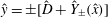
$-1$
along the fracture); the flow rate must be calculated. Our physical intuition about requiring a finite pressure drop to initiate flow along the fracture translates into the belief that there will be a critical value, say
 $Y=Y_{c}$
, that separates flowing and static fractures. This notion will be made more precise below in § 4.2.
$Y=Y_{c}$
, that separates flowing and static fractures. This notion will be made more precise below in § 4.2.
As in either formulation described, the flow is a Stokes flow with a unique velocity solution, we expect that the solutions may be mapped to one another. Equivalence of the two formulations is established straightforwardly by rescaling, from which we deduce
 $$\begin{eqnarray}Y=L\frac{B}{\unicode[STIX]{x0394}p}=Bq^{\ast },\quad 2q^{\ast }=\int _{-1-y_{-}(x)}^{1+y_{+}(x)}u_{1}^{\ast }(x,y)\,\text{d}y,\end{eqnarray}$$
i.e.
 $2q^{\ast }$
is the areal flow rate from the imposed pressure formulation, which is equivalent to the inverse of the mean pressure gradient,
$2q^{\ast }$
is the areal flow rate from the imposed pressure formulation, which is equivalent to the inverse of the mean pressure gradient,
 $L/\unicode[STIX]{x0394}p$
, computed in the imposed velocity formulation.
$L/\unicode[STIX]{x0394}p$
, computed in the imposed velocity formulation.
Although it is quite possible to compute
 $\boldsymbol{u}^{\ast }$
from the imposed pressure formulation and then vary
$\boldsymbol{u}^{\ast }$
from the imposed pressure formulation and then vary
 $Y$
to study the limit of no flow, numerically this is less well conditioned than using the fixed flow rate formulation. Since the computational method is iterative and has tolerances imposed for convergence, it proves easier to impose a tolerance on an iteration for which
$Y$
to study the limit of no flow, numerically this is less well conditioned than using the fixed flow rate formulation. Since the computational method is iterative and has tolerances imposed for convergence, it proves easier to impose a tolerance on an iteration for which
 $\boldsymbol{u}\sim O(1)$
than where
$\boldsymbol{u}\sim O(1)$
than where
 $\boldsymbol{u}^{\ast }\rightarrow 0$
. The identity (4.2) shows that it is feasible to work in this way. Using the imposed flow formulation, we find
$\boldsymbol{u}^{\ast }\rightarrow 0$
. The identity (4.2) shows that it is feasible to work in this way. Using the imposed flow formulation, we find
 $\unicode[STIX]{x0394}p$
as part of the solution and monitor convergence of
$\unicode[STIX]{x0394}p$
as part of the solution and monitor convergence of
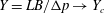 $Y=LB/\unicode[STIX]{x0394}p\rightarrow Y_{c}$
as we increase
$Y=LB/\unicode[STIX]{x0394}p\rightarrow Y_{c}$
as we increase
 $B$
. We also see that if a critical stress balance is achieved,
$B$
. We also see that if a critical stress balance is achieved,
 $\boldsymbol{u}^{\ast }\rightarrow 0$
(i.e. as
$\boldsymbol{u}^{\ast }\rightarrow 0$
(i.e. as
 $Y\rightarrow Y_{c}$
), then implicitly
$Y\rightarrow Y_{c}$
), then implicitly
 $q^{\ast }\sim B^{-1}$
as
$q^{\ast }\sim B^{-1}$
as
 $B\rightarrow \infty$
.
$B\rightarrow \infty$
.
4.1 Examples
We now examine three example sequences where we take increasingly large
 $B$
at fixed geometry, to understand the limiting behaviour. For simplicity we fix
$B$
at fixed geometry, to understand the limiting behaviour. For simplicity we fix
 $\unicode[STIX]{x1D713}=0$
. Figure 9 shows a relatively short fracture (
$\unicode[STIX]{x1D713}=0$
. Figure 9 shows a relatively short fracture (
 $H=1.5,~L=4$
) at
$H=1.5,~L=4$
) at
 $B=10,~100,~1000$
. Even at
$B=10,~100,~1000$
. Even at
 $B=10$
, the majority of the flow is unyielded, with stationary fouling regions filling the deep parts of the fracture and an intact plug moving along the centre. These regions are separated by a thin shear layer that extends between the narrowest parts of the fracture, widening slightly at the deepest parts. As
$B=10$
, the majority of the flow is unyielded, with stationary fouling regions filling the deep parts of the fracture and an intact plug moving along the centre. These regions are separated by a thin shear layer that extends between the narrowest parts of the fracture, widening slightly at the deepest parts. As
 $B$
increases, the width of this sheared layer is reduced, albeit slowly.
$B$
increases, the width of this sheared layer is reduced, albeit slowly.

Figure 9. Colourmap of the speed with superimposed streamlines in a relatively short fracture
 $H=1.5,~L=4$
: increasing
$H=1.5,~L=4$
: increasing
 $B=10,~100,~1000$
(from a to c). Unyielded regions are shown in grey.
$B=10,~100,~1000$
(from a to c). Unyielded regions are shown in grey.
Next, we consider a relatively long fracture with small
 $H/L$
(
$H/L$
(
 $H=0.1,~L=20$
); see figure 10. The flow has unyielded plug regions at the narrowest and widest parts of the fracture, but no static fouling layers in the deepest parts of the fracture. The plug in the widest part is moving more slowly than that in the narrowest part, and these two plugs remain separated as
$H=0.1,~L=20$
); see figure 10. The flow has unyielded plug regions at the narrowest and widest parts of the fracture, but no static fouling layers in the deepest parts of the fracture. The plug in the widest part is moving more slowly than that in the narrowest part, and these two plugs remain separated as
 $B$
is increased.
$B$
is increased.

Figure 10. Colourmap of the speed with superimposed streamlines in a relatively short fracture
 $H=0.1,~L=20$
: increasing
$H=0.1,~L=20$
: increasing
 $B=10,~100,~1000$
(from a to c). Unyielded regions are shown in grey.
$B=10,~100,~1000$
(from a to c). Unyielded regions are shown in grey.
Finally, we consider a more intermediate geometry (
 $H=2,~L=20$
); see figure 11. As may be expected, the limiting process at large
$H=2,~L=20$
); see figure 11. As may be expected, the limiting process at large
 $B$
is qualitatively somewhere between the previous two examples. The narrowest and widest parts of the fracture have moving central plug regions, but there is also a static fouling layer in the deepest part of the fracture, extending between say
$B$
is qualitatively somewhere between the previous two examples. The narrowest and widest parts of the fracture have moving central plug regions, but there is also a static fouling layer in the deepest part of the fracture, extending between say
 $x\in (-x_{f},x_{f})$
. The fouling layer and central plug are separated by a shear layer, which decreases slowly in width as
$x\in (-x_{f},x_{f})$
. The fouling layer and central plug are separated by a shear layer, which decreases slowly in width as
 $B$
increases (similarly to the short fracture). The length
$B$
increases (similarly to the short fracture). The length
 $x_{f}$
appears to approach a constant value as
$x_{f}$
appears to approach a constant value as
 $B$
increases. Similarly to the long fracture, the narrow and wide plugs remain separated at large
$B$
increases. Similarly to the long fracture, the narrow and wide plugs remain separated at large
 $B$
, moving at different speeds.
$B$
, moving at different speeds.

Figure 11. Colourmap of the speed with superimposed streamlines in a relatively short fracture
 $H=2,~L=20$
: increasing
$H=2,~L=20$
: increasing
 $B=10,~100,~1000$
(from a to c). Unyielded regions are shown in grey.
$B=10,~100,~1000$
(from a to c). Unyielded regions are shown in grey.
Figure 12 plots the variation of
 $Y$
and
$Y$
and
 $\unicode[STIX]{x0394}P/L$
, with increasing
$\unicode[STIX]{x0394}P/L$
, with increasing
 $B$
, for the three geometries illustrated in figures 9–11. We see that in all cases the computed
$B$
, for the three geometries illustrated in figures 9–11. We see that in all cases the computed
 $Y$
appears to asymptote to a constant value at large
$Y$
appears to asymptote to a constant value at large
 $B$
. This value denotes the critical limit
$B$
. This value denotes the critical limit
 $Y_{c}$
. Interestingly, the short and long fractures appear to asymptote to
$Y_{c}$
. Interestingly, the short and long fractures appear to asymptote to
 $Y_{c}\approx 1$
, whereas the intermediate geometry asymptotes to a value that is significantly larger. These examples are typical of the behaviour found over the whole range of our results.
$Y_{c}\approx 1$
, whereas the intermediate geometry asymptotes to a value that is significantly larger. These examples are typical of the behaviour found over the whole range of our results.


4.2 The critical limit from a variational method
We now define the critical limit more precisely. Use of the imposed pressure formulation has some advantages for this, as we may use standard variational techniques (e.g. Putz & Frigaard Reference Putz and Frigaard2010) to consider the zero flow limit. The solution
 $\boldsymbol{u}^{\ast }$
satisfies
$\boldsymbol{u}^{\ast }$
satisfies
 $$\begin{eqnarray}\displaystyle 0\leqslant a(\boldsymbol{u}^{\ast },\boldsymbol{u}^{\ast }) & = & \displaystyle -Y\;j(\boldsymbol{u}^{\ast })+L\int _{-1-y_{-}(x)}^{1+y_{+}(x)}u_{1}^{\ast }(x,y)\,\text{d}y\end{eqnarray}$$
 $$\begin{eqnarray}\displaystyle & = & \displaystyle -Y\;j(\boldsymbol{u}^{\ast })+\int _{-L/2}^{L/2}\int _{-1-y_{-}(x)}^{1+y_{+}(x)}u_{1}^{\ast }(x,y)\,\text{d}y\,\text{d}x=Y\;j(\boldsymbol{u}^{\ast })+Q(\boldsymbol{u}^{\ast }).\end{eqnarray}$$
The functionals
 $a(\boldsymbol{u}^{\ast },\boldsymbol{u}^{\ast })$
and
$a(\boldsymbol{u}^{\ast },\boldsymbol{u}^{\ast })$
and
 $j(\boldsymbol{u}^{\ast })$
denote respectively the viscous and plastic dissipation rate functionals:
$j(\boldsymbol{u}^{\ast })$
denote respectively the viscous and plastic dissipation rate functionals:
 $$\begin{eqnarray}\displaystyle & \displaystyle a(\boldsymbol{u}^{\ast },\boldsymbol{v}^{\ast })\equiv \int _{-L/2}^{L/2}\int _{-1-y_{-}(x)}^{1+y_{+}(x)}\frac{1}{2}\dot{\unicode[STIX]{x1D6FE}}_{ij}(\boldsymbol{u}^{\ast })\dot{\unicode[STIX]{x1D6FE}}_{ij}(\boldsymbol{v}^{\ast })\,\text{d}y\,\text{d}x,\quad \boldsymbol{u}^{\ast },\boldsymbol{v}^{\ast }\in \mathscr{V}, & \displaystyle\end{eqnarray}$$
 $$\begin{eqnarray}\displaystyle & \displaystyle j(\boldsymbol{v}^{\ast })\equiv \int _{-L/2}^{L/2}\int _{-1-y_{-}(x)}^{1+y_{+}(x)}\dot{\unicode[STIX]{x1D6FE}}(\boldsymbol{v}^{\ast })\,\text{d}y\,\text{d}x,\quad \boldsymbol{v}^{\ast }\in \mathscr{V}. & \displaystyle\end{eqnarray}$$
It should be noted that we have extended the velocity integral at the inflow to the entire fracture:
 $$\begin{eqnarray}Q(\boldsymbol{u}^{\ast })\equiv \int _{-L/2}^{L/2}\int _{-1-y_{-}(x)}^{1+y_{+}(x)}u_{1}^{\ast }(x,y)\,\text{d}y\,\text{d}x,\end{eqnarray}$$
as the flow rate is identical through each cross-section. Continuing this analysis,
 $$\begin{eqnarray}0\leqslant a(\boldsymbol{u}^{\ast },\boldsymbol{u}^{\ast })\leqslant -j(\boldsymbol{u}^{\ast })\left[Y-\sup _{\boldsymbol{ v}\ast \in \mathscr{V},\boldsymbol{v}\ast \not =0}\frac{Q(\boldsymbol{v}^{\ast })}{j(\boldsymbol{v}^{\ast })}\right]\equiv -j(\boldsymbol{u}^{\ast })\left[Y-Y_{c}\right],\end{eqnarray}$$
where
 $\mathscr{V}$
denotes the space of admissible velocity solutions. The critical value of
$\mathscr{V}$
denotes the space of admissible velocity solutions. The critical value of
 $Y$
is thus formally defined as
$Y$
is thus formally defined as
 $$\begin{eqnarray}Y_{c}=\sup _{\boldsymbol{v}\ast \in \mathscr{V},\boldsymbol{v}\ast \not =0}\frac{Q(\boldsymbol{v}^{\ast })}{j(\boldsymbol{v}^{\ast })}.\end{eqnarray}$$
Following a similar procedure to Putz & Frigaard (Reference Putz and Frigaard2010) we can show that
 $$\begin{eqnarray}\displaystyle & \displaystyle a(\boldsymbol{u}^{\ast },\boldsymbol{u}^{\ast })\sim O([Y_{c}-Y]^{2})\quad \text{as }Y\rightarrow Y_{c}^{\ast -}, & \displaystyle\end{eqnarray}$$
 $$\begin{eqnarray}\displaystyle & \displaystyle Yj(\boldsymbol{u}^{\ast })\sim Q(\boldsymbol{u}^{\ast })\sim O(Y_{c}-Y)\quad \text{as }Y\rightarrow Y_{c}^{\ast -}, & \displaystyle\end{eqnarray}$$
 $$\begin{eqnarray}\displaystyle & \displaystyle j(\boldsymbol{u}^{\ast })\gtrsim \frac{a(\boldsymbol{u}^{\ast },\boldsymbol{u}^{\ast })}{[Y_{c}-Y]}\geqslant 0\quad \text{as }Y\rightarrow Y_{c}^{\ast -}. & \displaystyle\end{eqnarray}$$
Figure 13 shows the computed values of
 $a(u^{\ast },u^{\ast })$
,
$a(u^{\ast },u^{\ast })$
,
 $j(u^{\ast })$
and
$j(u^{\ast })$
and
 $Q(u^{\ast })$
as
$Q(u^{\ast })$
as
 $B$
is increased, for the three geometries illustrated in figures 9–11. We see that
$B$
is increased, for the three geometries illustrated in figures 9–11. We see that
 $a(u^{\ast },u^{\ast })$
does indeed converge much faster than
$a(u^{\ast },u^{\ast })$
does indeed converge much faster than
 $j(u^{\ast })$
and
$j(u^{\ast })$
and
 $Q(u^{\ast })$
, as is implicit in the above bounds. It should be noted that the
$Q(u^{\ast })$
, as is implicit in the above bounds. It should be noted that the
 $O([Y_{c}-Y]^{2})$
in (4.12) is a lower bound on the decay rate of the viscous dissipation, and we can see that the decay rate is indeed faster than quadratic. Equation (4.14) ensures that the plastic dissipation decays to zero at least one order slower, and (4.13) ensures that the limiting balance is between the plastic dissipation and the flow rate. We again observe this in figure 13. This in turn can be used to argue that the supremum in (4.11) is in fact achieved by the solution. Indeed, if one knows the distribution of the limiting velocity solution, this can be used to estimate
$O([Y_{c}-Y]^{2})$
in (4.12) is a lower bound on the decay rate of the viscous dissipation, and we can see that the decay rate is indeed faster than quadratic. Equation (4.14) ensures that the plastic dissipation decays to zero at least one order slower, and (4.13) ensures that the limiting balance is between the plastic dissipation and the flow rate. We again observe this in figure 13. This in turn can be used to argue that the supremum in (4.11) is in fact achieved by the solution. Indeed, if one knows the distribution of the limiting velocity solution, this can be used to estimate
 $Y_{c}$
by inserting in (4.11). It should be noted that the size of the limiting velocity is not important in this determination as (4.11) is scale-invariant.
$Y_{c}$
by inserting in (4.11). It should be noted that the size of the limiting velocity is not important in this determination as (4.11) is scale-invariant.


For computing the velocity, especially numerically, it can be more convenient to work with
 $O(1)$
quantities, e.g. in tracking convergence. In moving between formulations it is necessary to rescale velocities with
$O(1)$
quantities, e.g. in tracking convergence. In moving between formulations it is necessary to rescale velocities with
 $q^{\ast }$
. Thus, to evaluate
$q^{\ast }$
. Thus, to evaluate
 $Y_{c}$
by inserting the limiting solution
$Y_{c}$
by inserting the limiting solution
 $\boldsymbol{u}^{\ast }$
into (4.11), we may instead work directly with
$\boldsymbol{u}^{\ast }$
into (4.11), we may instead work directly with
 $\boldsymbol{u}$
in the large
$\boldsymbol{u}$
in the large
 $B$
limit, i.e.
$B$
limit, i.e.
 $$\begin{eqnarray}Y_{c}\sim \lim _{B\rightarrow \infty }\frac{Q(\boldsymbol{u})}{j(\boldsymbol{u})}=\lim _{B\rightarrow \infty }\frac{2L}{j(\boldsymbol{u})},\end{eqnarray}$$
on noting that
 $Q(\boldsymbol{u})=2L$
in the fixed flow rate formulation. In the next section we will estimate
$Q(\boldsymbol{u})=2L$
in the fixed flow rate formulation. In the next section we will estimate
 $j(\boldsymbol{u})$
in order to derive approximations to
$j(\boldsymbol{u})$
in order to derive approximations to
 $Y_{c}$
.
$Y_{c}$
.
4.3 Characteristics of the different geometries
The flows illustrated in figures 9–11 represent the range of all observed behaviours (at least for
 $\unicode[STIX]{x1D6F9}=1$
). By exploring these flows numerically as
$\unicode[STIX]{x1D6F9}=1$
). By exploring these flows numerically as
 $B$
is increased, we have been able to understand the different flow structures that emerge and in this way estimate the dominant contributions to
$B$
is increased, we have been able to understand the different flow structures that emerge and in this way estimate the dominant contributions to
 $j(\boldsymbol{u})$
from each type of flow. This leads to a prediction of
$j(\boldsymbol{u})$
from each type of flow. This leads to a prediction of
 $Y_{c}$
for the different fracture geometries. A summary of the results of this analysis follows, with the details confined to a number of appendices.
$Y_{c}$
for the different fracture geometries. A summary of the results of this analysis follows, with the details confined to a number of appendices.
Short fractures. By short fractures we mean fractures in which we have observed a single central plug region along the fracture as
 $B\rightarrow \infty$
, e.g. figure 9. The analysis of short fractures is presented in appendix A. We are able to deduce that these flows approach the same limit as that of a uniform channel, hence
$B\rightarrow \infty$
, e.g. figure 9. The analysis of short fractures is presented in appendix A. We are able to deduce that these flows approach the same limit as that of a uniform channel, hence
 $Y_{c}=1$
. However, the approach to the limit differs from that of a straight channel. As
$Y_{c}=1$
. However, the approach to the limit differs from that of a straight channel. As
 $B\rightarrow \infty$
,
$B\rightarrow \infty$
,
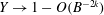 $Y\rightarrow 1-O(B^{-2k})$
and
$Y\rightarrow 1-O(B^{-2k})$
and
 $d_{0}\sim B^{-k}$
for some
$d_{0}\sim B^{-k}$
for some
 $k\in [1/3,0.4]$
. Here,
$k\in [1/3,0.4]$
. Here,
 $d_{0}$
represents the maximal width of the thin yielded shear layers observed. Figure 14 explores this convergence from our numerical results, taken from five different short fracture geometries, each as
$d_{0}$
represents the maximal width of the thin yielded shear layers observed. Figure 14 explores this convergence from our numerical results, taken from five different short fracture geometries, each as
 $B$
is increased. It appears that, in fact,
$B$
is increased. It appears that, in fact,
 $d_{0}\sim B^{-1/3}$
and
$d_{0}\sim B^{-1/3}$
and
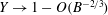 $Y\rightarrow 1-O(B^{-2/3})$
, in accordance with this analysis. It should be noted that in a plane channel flow of a Bingham fluid, from the analytical solution as
$Y\rightarrow 1-O(B^{-2/3})$
, in accordance with this analysis. It should be noted that in a plane channel flow of a Bingham fluid, from the analytical solution as
 $B\rightarrow \infty$
we find
$B\rightarrow \infty$
we find
 $d_{0}\sim B^{-1/2}$
. Here, the yielded layer is different, being non-uniform and influenced by extensional stresses.
$d_{0}\sim B^{-1/2}$
. Here, the yielded layer is different, being non-uniform and influenced by extensional stresses.

Figure 14. Limiting behaviour as
 $B\rightarrow \infty$
for five short fracture geometries: (a) shear layer thickness
$B\rightarrow \infty$
for five short fracture geometries: (a) shear layer thickness
 $d_{0}$
; (b)
$d_{0}$
; (b)
 $Y_{c}-Y$
. Data are shown for (○,
$Y_{c}-Y$
. Data are shown for (○,
 $H=1,L=3$
), (▫,
$H=1,L=3$
), (▫,
 $H=0.5$
,
$H=0.5$
,
 $L=2$
), (▵,
$L=2$
), (▵,
 $H=0.25,L=4$
), (*,
$H=0.25,L=4$
), (*,
 $H=3,L=2$
),
$H=3,L=2$
),
 $(+,H=4,L=4)$
; recall that
$(+,H=4,L=4)$
; recall that
 $Y_{c}=1$
for short fractures.
$Y_{c}=1$
for short fractures.
Long fractures with no fouling. The analysis of long fractures is presented in appendix B. We are able to deduce that
 $$\begin{eqnarray}Y_{c}=\frac{1}{L}\int _{-L/2}^{L/2}\frac{1}{1+h}\,\text{d}x.\end{eqnarray}$$
From the analysis we find
 $Y_{c}-Y\sim B^{-1/2}$
as
$Y_{c}-Y\sim B^{-1/2}$
as
 $B\rightarrow \infty$
, i.e. faster than convergence with
$B\rightarrow \infty$
, i.e. faster than convergence with
 $B$
for the short fractures. Figure 15 illustrates the convergence rate of
$B$
for the short fractures. Figure 15 illustrates the convergence rate of
 $Y_{c}-Y$
as
$Y_{c}-Y$
as
 $B\rightarrow \infty$
for one of our computed ‘long’ fractures. The
$B\rightarrow \infty$
for one of our computed ‘long’ fractures. The
 $B^{-1/2}$
scaling is verified.
$B^{-1/2}$
scaling is verified.

Figure 15. Convergence of
 $Y_{c}-Y$
(
$Y_{c}-Y$
(
 $Y_{c}=1.227$
) as
$Y_{c}=1.227$
) as
 $B\rightarrow \infty$
for
$B\rightarrow \infty$
for
 $H=1$
,
$H=1$
,
 $L=20$
.
$L=20$
.
Intermediate fractures with partial fouling. We have seen that for both short and long fractures, it is possible to estimate the critical limit, essentially by using (3.2). For sufficiently short periodic fractures, the flow yields at the narrowest width, which means that (3.2) can be used, taking the modified fracture width from (3.6), which amounts to
 $h(x)\rightarrow 0$
as
$h(x)\rightarrow 0$
as
 $B\rightarrow \infty$
. For long enough fractures, no fouling occurs and (3.2) is applied directly. However, as we have seen in figure 11, for intermediate
$B\rightarrow \infty$
. For long enough fractures, no fouling occurs and (3.2) is applied directly. However, as we have seen in figure 11, for intermediate
 $H/L$
, the limit
$H/L$
, the limit
 $B\rightarrow \infty$
results in only a limited portion of the fracture being fouled, say
$B\rightarrow \infty$
results in only a limited portion of the fracture being fouled, say
 $x\in [-x_{f},x_{f}]$
for a symmetric fracture (
$x\in [-x_{f},x_{f}]$
for a symmetric fracture (
 $\unicode[STIX]{x1D713}=0$
). So far it is unclear (i) how to predict
$\unicode[STIX]{x1D713}=0$
). So far it is unclear (i) how to predict
 $Y_{c}$
for such intermediate fractures, (ii) how the fouling length
$Y_{c}$
for such intermediate fractures, (ii) how the fouling length
 $x_{f}$
is determined and (iii) what determines transitions from nominally short to intermediate to long fractures.
$x_{f}$
is determined and (iii) what determines transitions from nominally short to intermediate to long fractures.
One feature observed in, e.g., figure 11 is that for intermediate
 $H/L$
a significant portion of the fracture length remains yielded in the limit
$H/L$
a significant portion of the fracture length remains yielded in the limit
 $B\rightarrow \infty$
. Indeed, the limiting solutions appear to result in true unyielded regions only in the narrowest and widest parts of the fracture (approximately
$B\rightarrow \infty$
. Indeed, the limiting solutions appear to result in true unyielded regions only in the narrowest and widest parts of the fracture (approximately
 $x\in [-x_{f},x_{f}]$
), with a sheared pseudo-plug region in between. The pseudo-plug region is of course necessary, since the true plug speeds in wide and narrow parts of the fracture are different. This type of pseudo-plug region arises in many viscoplastic flows
$x\in [-x_{f},x_{f}]$
), with a sheared pseudo-plug region in between. The pseudo-plug region is of course necessary, since the true plug speeds in wide and narrow parts of the fracture are different. This type of pseudo-plug region arises in many viscoplastic flows
In appendix C, we first analyse the pseudo-plug, assuming that it is a lubrication flow limit (§ C.1), but discover that, in fact, the stress and velocity distributions are not compatible with this interpretation. This leads us to an empirical approach in which we fit a leading-order expression to the stress field (§ C.2). This understanding of the solution leads us, via an estimation of the plastic dissipation functional, to an approximation of
 $Y$
as a function of the unknown
$Y$
as a function of the unknown
 $x_{f}$
, as
$x_{f}$
, as
 $B\rightarrow \infty$
:
$B\rightarrow \infty$
:
 $$\begin{eqnarray}\displaystyle Y(x_{f})\sim \frac{Q(\boldsymbol{u})}{j(\boldsymbol{u})}\approx \frac{L/2}{\displaystyle \int _{x_{f}}^{L/2}\frac{1}{1+h(x)}\,\text{d}x+\frac{x_{f}}{1+h(x_{f})}+\unicode[STIX]{x03C0}\ln (1+h(x_{f}))} & & \displaystyle\end{eqnarray}$$
(see § C.3). If we regard
 $x_{f}$
as being selected by minimizing the strain rate, the actual
$x_{f}$
as being selected by minimizing the strain rate, the actual
 $x_{f}$
is determined by maximizing
$x_{f}$
is determined by maximizing
 $Y(x_{f})$
with respect to
$Y(x_{f})$
with respect to
 $x_{f}$
, thus giving
$x_{f}$
, thus giving
 $Y_{c}$
. It should be noted that the first two terms in the denominator of (4.17) effectively interpolate between the limiting
$Y_{c}$
. It should be noted that the first two terms in the denominator of (4.17) effectively interpolate between the limiting
 $Y_{c}$
derived for short channels (
$Y_{c}$
derived for short channels (
 $x_{f}\rightarrow L/2$
) and that for long channels with no fouling (
$x_{f}\rightarrow L/2$
) and that for long channels with no fouling (
 $x_{f}\rightarrow 0$
). The third term in (4.17) also vanishes as
$x_{f}\rightarrow 0$
). The third term in (4.17) also vanishes as
 $x_{f}\rightarrow L/2$
, so that the expression for short channels is contained in (4.17).
$x_{f}\rightarrow L/2$
, so that the expression for short channels is contained in (4.17).
Figure 16(a) shows examples of the variation of
 $Y(x_{f})$
computed from (4.17) for
$Y(x_{f})$
computed from (4.17) for
 $L=20$
,
$L=20$
,
 $H=0,1,\ldots ,8$
(black), and
$H=0,1,\ldots ,8$
(black), and
 $L=6$
,
$L=6$
,
 $H=0,~0.25,~0.5,\ldots ,2$
(red). The maximum of
$H=0,~0.25,~0.5,\ldots ,2$
(red). The maximum of
 $Y(x_{f})$
is attained either at an endpoint or at the zero of
$Y(x_{f})$
is attained either at an endpoint or at the zero of
 $$\begin{eqnarray}x_{f}=\unicode[STIX]{x03C0}(1+h(x_{f})),\end{eqnarray}$$
which is straightforwardly computed. For the examples shown, for
 $L=6$
the maximum is
$L=6$
the maximum is
 $Y_{c}=1$
, attained at
$Y_{c}=1$
, attained at
 $x_{f}=L/2$
, for all
$x_{f}=L/2$
, for all
 $H$
. As
$H$
. As
 $(1+h(x_{f}))\in [1,1+H]$
, we see that the above equation has a root only for
$(1+h(x_{f}))\in [1,1+H]$
, we see that the above equation has a root only for
 $L>2\unicode[STIX]{x03C0}$
. Since when this is not satisfied we find
$L>2\unicode[STIX]{x03C0}$
. Since when this is not satisfied we find
 $Y_{c}=1$
, which is the short-fracture limit, we adopt the condition
$Y_{c}=1$
, which is the short-fracture limit, we adopt the condition
 $$\begin{eqnarray}L<2\unicode[STIX]{x03C0}\end{eqnarray}$$
as our definition of short fractures. At larger
 $L$
we see that there is a maximum in
$L$
we see that there is a maximum in
 $(0,L/2)$
and compute this numerically. As
$(0,L/2)$
and compute this numerically. As
 $L\rightarrow \infty$
we find that
$L\rightarrow \infty$
we find that
 $2x_{f}/L\rightarrow 0$
since
$2x_{f}/L\rightarrow 0$
since
 $x_{f}\rightarrow (1+H)\unicode[STIX]{x03C0}$
. The second and third terms in the denominator of (4.17) then become
$x_{f}\rightarrow (1+H)\unicode[STIX]{x03C0}$
. The second and third terms in the denominator of (4.17) then become
 $O(1/L)$
smaller than the first one, which converges to
$O(1/L)$
smaller than the first one, which converges to
 $Y_{c}$
for the long-fracture limit without fouling. Figure 16(b) shows the variation of
$Y_{c}$
for the long-fracture limit without fouling. Figure 16(b) shows the variation of
 $Y_{c}$
with
$Y_{c}$
with
 $L$
for two values of
$L$
for two values of
 $H$
, computed as the maximum of (4.17). For
$H$
, computed as the maximum of (4.17). For
 $L$
satisfying (4.19) we see that
$L$
satisfying (4.19) we see that
 $Y_{c}=1$
, increasing smoothly to the asymptotic values for no fouling at large
$Y_{c}=1$
, increasing smoothly to the asymptotic values for no fouling at large
 $L$
, marked with the broken lines.
$L$
, marked with the broken lines.

Figure 16. (a) Variation of
 $Y(x_{f})$
from (4.17) for
$Y(x_{f})$
from (4.17) for
 $L=20$
,
$L=20$
,
 $H=0,~1,\ldots ,8$
(black);
$H=0,~1,\ldots ,8$
(black);
 $L=6$
,
$L=6$
,
 $H=0,~0.25,~0.5,\ldots ,2$
(red). (b) Variation of
$H=0,~0.25,~0.5,\ldots ,2$
(red). (b) Variation of
 $Y_{c}$
(computed by maximizing
$Y_{c}$
(computed by maximizing
 $Y(x_{f})$
in (4.17)) with
$Y(x_{f})$
in (4.17)) with
 $L$
for
$L$
for
 $H=1$
(black) and
$H=1$
(black) and
 $H=4$
(red). Broken lines indicate the limit of
$H=4$
(red). Broken lines indicate the limit of
 $Y_{c}$
with no fouling.
$Y_{c}$
with no fouling.
We have computed
 $Y_{c}$
from this toy model, by maximizing (4.17) over
$Y_{c}$
from this toy model, by maximizing (4.17) over
 $x_{f}$
, and compare this with the values of
$x_{f}$
, and compare this with the values of
 $Y_{c}$
from our 2D computations. The agreement is reasonable, as is shown in figure 23 in § C.3. Although reasonable, it is possible to improve (4.17) by a better estimate of
$Y_{c}$
from our 2D computations. The agreement is reasonable, as is shown in figure 23 in § C.3. Although reasonable, it is possible to improve (4.17) by a better estimate of
 $j(\boldsymbol{u})$
in which the pseudo-plug stresses use a more accurate approximation. This derivation is detailed in § C.4, resulting in
$j(\boldsymbol{u})$
in which the pseudo-plug stresses use a more accurate approximation. This derivation is detailed in § C.4, resulting in
 $$\begin{eqnarray}Y(x_{f})\sim \frac{Q(\boldsymbol{u})}{j(\boldsymbol{u})}\approx \frac{L/2}{\displaystyle \int _{x_{f}}^{L/2}\frac{1}{1+h(x)}\,\text{d}x+\frac{x_{f}}{1+h(x_{f})}+\unicode[STIX]{x03C0}\int _{x_{f}}^{L/2}\frac{|h^{\prime }|}{(1+h)}\frac{1}{1+\sqrt{f_{0}|h^{\prime }|}}\,\text{d}x},\end{eqnarray}$$
where
 $f_{0}$
is a constant (see § C.4). We again find
$f_{0}$
is a constant (see § C.4). We again find
 $x_{f}$
by maximizing
$x_{f}$
by maximizing
 $Y_{x_{f}}$
. This results in
$Y_{x_{f}}$
. This results in
 $Y_{c}$
and
$Y_{c}$
and
 $x_{f}$
as illustrated in figure 17(a,b) respectively. We observe a general increase in
$x_{f}$
as illustrated in figure 17(a,b) respectively. We observe a general increase in
 $Y_{c}$
and a small shift in
$Y_{c}$
and a small shift in
 $x_{f}$
compared with (4.17). The relative error with the computed 2D results is however diminished, see figure 17(c), now typically remaining below 10 % for most of the parameter space.
$x_{f}$
compared with (4.17). The relative error with the computed 2D results is however diminished, see figure 17(c), now typically remaining below 10 % for most of the parameter space.


4.4 Affine fractures
Finally, we present some examples of the limiting process in affine fractures. Three different styles of affine fracture are generated for intermediate
 $H=2$
,
$H=2$
,
 $L=20$
. Figure 5 earlier and figures 18 and 19 below present the sequence
$L=20$
. Figure 5 earlier and figures 18 and 19 below present the sequence
 $B=100,~1000,~10\,000$
for each fracture, plotting the speed, streamlines and unyielded plug regions. In general, we observe that the small-scale fracture roughness is always fouled. As
$B=100,~1000,~10\,000$
for each fracture, plotting the speed, streamlines and unyielded plug regions. In general, we observe that the small-scale fracture roughness is always fouled. As
 $B$
increases, a larger fraction of the fracture becomes immobilized. The boundaries of the flowing part of the fracture are formed by arc-like surfaces that span between locally narrow points of the fracture wall. The radius of curvature of these surfaces increases with
$B$
increases, a larger fraction of the fracture becomes immobilized. The boundaries of the flowing part of the fracture are formed by arc-like surfaces that span between locally narrow points of the fracture wall. The radius of curvature of these surfaces increases with
 $B$
.
$B$
.

Figure 18. Computed examples of speed
 $|\boldsymbol{u}|$
and streamlines for a fracture formed from two different affine surfaces. The parameters are
$|\boldsymbol{u}|$
and streamlines for a fracture formed from two different affine surfaces. The parameters are
 $H=2$
,
$H=2$
,
 $L=20$
,
$L=20$
,
 $B=100,~1000,~10\,000$
, from (a) to (c), with (grey) unyielded plugs.
$B=100,~1000,~10\,000$
, from (a) to (c), with (grey) unyielded plugs.

Figure 19. Computed examples of speed
 $|\boldsymbol{u}|$
and streamlines for a fracture formed from two identical affine surfaces, shifted. The parameters are
$|\boldsymbol{u}|$
and streamlines for a fracture formed from two identical affine surfaces, shifted. The parameters are
 $H=2$
,
$H=2$
,
 $L=20$
,
$L=20$
,
 $B=100,~1000,~10\,000$
, from (a) to (c), with (grey) unyielded plugs.
$B=100,~1000,~10\,000$
, from (a) to (c), with (grey) unyielded plugs.
It is notable that as
 $B$
increases, the self-selected flowing channel geometry consists of a series of joined segments along which the streamlines are approximately parallel. In such sections, shear components evidently dominate. These parallel segments are connected by angular converging and diverging segments, in which extensional stresses and strain rates will be significant. The limiting process as
$B$
increases, the self-selected flowing channel geometry consists of a series of joined segments along which the streamlines are approximately parallel. In such sections, shear components evidently dominate. These parallel segments are connected by angular converging and diverging segments, in which extensional stresses and strain rates will be significant. The limiting process as
 $B\rightarrow \infty$
appears to result again in a combination of thin yielded shear layers and non-vanishing
$B\rightarrow \infty$
appears to result again in a combination of thin yielded shear layers and non-vanishing
 $O(1)$
pseudo-plug regions. Although the evident complexity of the self-selection and limiting processes so far eludes a simple explanation, there is some hope that these component structures can be understood. Thus, if one can first understand the geometric features of flow self-selection (meaning the fouling process and orientation of the flowing part of the fracture, generating tortuosity) it should be possible to estimate the critical pressure drops (or yield stresses).
$O(1)$
pseudo-plug regions. Although the evident complexity of the self-selection and limiting processes so far eludes a simple explanation, there is some hope that these component structures can be understood. Thus, if one can first understand the geometric features of flow self-selection (meaning the fouling process and orientation of the flowing part of the fracture, generating tortuosity) it should be possible to estimate the critical pressure drops (or yield stresses).
More quantitatively, we may evaluate
 $Y_{c}$
for these geometries from the computed 2D solution. Figure 20 shows convergence of
$Y_{c}$
for these geometries from the computed 2D solution. Figure 20 shows convergence of
 $Y\rightarrow Y_{c}$
as
$Y\rightarrow Y_{c}$
as
 $B\rightarrow \infty$
. The symmetric fracture has the smallest
$B\rightarrow \infty$
. The symmetric fracture has the smallest
 $Y_{c}$
, and also appears to have the more constricted flow apertures. The other two geometries appear to compensate increasing tortuosity (smaller
$Y_{c}$
, and also appears to have the more constricted flow apertures. The other two geometries appear to compensate increasing tortuosity (smaller
 $Y$
) with a larger effective channel width (larger
$Y$
) with a larger effective channel width (larger
 $Y$
).
$Y$
).

Figure 20. Computed yield number as a function of the Bingham number for the three different affine fractures of figures 5–19. Blue squares: the two surface are symmetrical. Red circles: the two surfaces are uncorrelated. Black lozenges: the two surfaces are identical, shifted laterally with a constant gap.
5 Discussion/conclusions
In this study we have investigated the two-dimensional flow of a Bingham fluid along an uneven fracture. The work has two principal foci. The first is to determine numerically the flow-rate–pressure-drop relationship in such geometries (the appropriate Darcy law), to understand better the limits of simple approximations that are presently used in a somewhat ad hoc manner. Second, we explore the limiting values of the pressure drop (equivalently yield stress) at which non-zero flows are first found. This question has critical consequences for the study of flow onset in pressure-driven porous media flows, i.e. selection of the critical initial path, as well as helping to provide practical estimates for invasive sealing of porous media/channels, i.e. how far will a sealing fluid penetrate under a given driving pressure?
The initial part of the paper has extensively studied geometric effects in idealized fractures (periodic with wavy or triangular profiles) of dimension
 $(H,L)$
. Strict application of lubrication/Hele-Shaw approximations to the flow to provide (nonlinear) Darcy-type flow laws has been shown to be limited to
$(H,L)$
. Strict application of lubrication/Hele-Shaw approximations to the flow to provide (nonlinear) Darcy-type flow laws has been shown to be limited to
 $H/L\ll 1$
, as may be expected. As a rule of thumb, errors of 10 % or less appear to require
$H/L\ll 1$
, as may be expected. As a rule of thumb, errors of 10 % or less appear to require
 $H/L\lessapprox 1/20$
. For geometries outside these limits, flow approximations are vulnerable to similar effects to Newtonian fluids, e.g. development of tortuosity, etc. One significant difference between Newtonian and Bingham (or other generalized Newtonian) fluids is in the coupling of geometrical and rheological parameters in the flow law. In the Newtonian fluid literature, there are many efforts to improve and extend Darcy-law-type estimates to these situations. Here, we have resisted the temptation to develop analogous methods. It is clear that some of these methods would be effective, especially in the limit of low
$H/L\lessapprox 1/20$
. For geometries outside these limits, flow approximations are vulnerable to similar effects to Newtonian fluids, e.g. development of tortuosity, etc. One significant difference between Newtonian and Bingham (or other generalized Newtonian) fluids is in the coupling of geometrical and rheological parameters in the flow law. In the Newtonian fluid literature, there are many efforts to improve and extend Darcy-law-type estimates to these situations. Here, we have resisted the temptation to develop analogous methods. It is clear that some of these methods would be effective, especially in the limit of low
 $B$
and for
$B$
and for
 $H/L$
increasing away from the lubrication limit, but infliction of this algebraic misery on the reader is left to other researchers.
$H/L$
increasing away from the lubrication limit, but infliction of this algebraic misery on the reader is left to other researchers.
Moving to larger
 $B$
or for
$B$
or for
 $H/L\not \ll 1$
, a more serious limitation of lubrication-type approximations to the Darcy law emerges. Unyielded fluid appears at the wall in deeper parts of the fracture (fouling layers). Fouling layers provide an
$H/L\not \ll 1$
, a more serious limitation of lubrication-type approximations to the Darcy law emerges. Unyielded fluid appears at the wall in deeper parts of the fracture (fouling layers). Fouling layers provide an
 $O(1)$
adjustment of the flowing area and hence
$O(1)$
adjustment of the flowing area and hence
 $O(1)$
errors in the predictions of lubrication-type approximations. We have demonstrated that these errors can be reduced significantly by adopting the yield surface of the fouling layers as the new fracture wall and applying the usual lubrication approximation. Therefore, approximation of the flow law presents no particular problem provided that the fouling layers are known. Unfortunately, this is not the case as the fluid self-selects the flowing area.
$O(1)$
errors in the predictions of lubrication-type approximations. We have demonstrated that these errors can be reduced significantly by adopting the yield surface of the fouling layers as the new fracture wall and applying the usual lubrication approximation. Therefore, approximation of the flow law presents no particular problem provided that the fouling layers are known. Unfortunately, this is not the case as the fluid self-selects the flowing area.
Previous work has addressed the question of the onset of fouling in idealized geometries with
 $O(1)$
variations (Roustaei & Frigaard Reference Roustaei and Frigaard2013; Roustaei et al.
Reference Roustaei, Gosselin and Frigaard2015). Smaller-scale roughness also seems to readily foul, although to the best of our knowledge this has not been quantified. At intermediate
$O(1)$
variations (Roustaei & Frigaard Reference Roustaei and Frigaard2013; Roustaei et al.
Reference Roustaei, Gosselin and Frigaard2015). Smaller-scale roughness also seems to readily foul, although to the best of our knowledge this has not been quantified. At intermediate
 $B$
, estimation of the degree of fouling appears to be difficult, as a general problem for which one would like to specify a simple predictive closure relationship. However, numerical solution as here is an effective tool even for the very complex affine geometries, and can be easily extended to more general yield stress fluid models. Although Newtonian fluids do not foul and self-select, sufficiently deep undulations do result in zones of recirculation. This link is explored in Roustaei & Frigaard (Reference Roustaei and Frigaard2013). Thus, except for very large
$B$
, estimation of the degree of fouling appears to be difficult, as a general problem for which one would like to specify a simple predictive closure relationship. However, numerical solution as here is an effective tool even for the very complex affine geometries, and can be easily extended to more general yield stress fluid models. Although Newtonian fluids do not foul and self-select, sufficiently deep undulations do result in zones of recirculation. This link is explored in Roustaei & Frigaard (Reference Roustaei and Frigaard2013). Thus, except for very large
 $B$
, it may be that the range of speeds encountered in Bingham and Newtonian fluids flowing through the same geometry may not differ significantly. This is also observed in packed-bed models of porous media at fixed flow rates (Chevalier et al.
Reference Chevalier, Chevalier, Clain, Dupla, Canou, Rodts and Coussot2013a
; Bleyer & Coussot Reference Bleyer and Coussot2014).
$B$
, it may be that the range of speeds encountered in Bingham and Newtonian fluids flowing through the same geometry may not differ significantly. This is also observed in packed-bed models of porous media at fixed flow rates (Chevalier et al.
Reference Chevalier, Chevalier, Clain, Dupla, Canou, Rodts and Coussot2013a
; Bleyer & Coussot Reference Bleyer and Coussot2014).
A significant part of the paper has considered the limit of no flow,
 $B\rightarrow \infty$
, which via a rescaling can be characterized with the yield number:
$B\rightarrow \infty$
, which via a rescaling can be characterized with the yield number:
 $$\begin{eqnarray}Y\equiv \frac{\hat{L}}{\hat{D}}\frac{\hat{\unicode[STIX]{x1D70F}}_{Y}}{\unicode[STIX]{x0394}\hat{P}},\end{eqnarray}$$
directly representing the balance between the applied pressure and the resisting yield stress. Above a critical value
 $Y_{c}$
there is no flow. On the theoretical side, we have formally characterized
$Y_{c}$
there is no flow. On the theoretical side, we have formally characterized
 $Y_{c}$
as a limiting ratio of flow rate to plastic dissipation, shown that this limit is attained by the velocity solution and provided general bounds on convergence of the viscous dissipation, plastic dissipation and flow rate in the limit
$Y_{c}$
as a limiting ratio of flow rate to plastic dissipation, shown that this limit is attained by the velocity solution and provided general bounds on convergence of the viscous dissipation, plastic dissipation and flow rate in the limit
 $Y\rightarrow Y_{c}^{-}$
. We have then studied the approach to
$Y\rightarrow Y_{c}^{-}$
. We have then studied the approach to
 $Y_{c}$
numerically and asymptotically for simpler symmetric fracture geometries, deriving the leading-order behaviour in the cases of both short and long–thin fractures.
$Y_{c}$
numerically and asymptotically for simpler symmetric fracture geometries, deriving the leading-order behaviour in the cases of both short and long–thin fractures.
For short fractures, we find that
 $Y_{c}=1$
: at large
$Y_{c}=1$
: at large
 $B$
the flow consists of an intact central plug region separated from the walls (and fouling layers) by a progressively thinning shear layer. This limit is analogous to the flow in a uniform channel, for which also
$B$
the flow consists of an intact central plug region separated from the walls (and fouling layers) by a progressively thinning shear layer. This limit is analogous to the flow in a uniform channel, for which also
 $Y_{c}=1$
. Short fractures, for the purposes of this limiting process, are defined as
$Y_{c}=1$
. Short fractures, for the purposes of this limiting process, are defined as
 $L<2\unicode[STIX]{x03C0}$
. For long–thin fractures, no fouling occurs and the lubrication approximation is valid. The critical yield number can be approximated from the harmonic mean of the fracture width. However, application of this naïve approximation more widely will incur
$L<2\unicode[STIX]{x03C0}$
. For long–thin fractures, no fouling occurs and the lubrication approximation is valid. The critical yield number can be approximated from the harmonic mean of the fracture width. However, application of this naïve approximation more widely will incur
 $O(1)$
errors, and we have seen that the lubrication approximation is quite limited.
$O(1)$
errors, and we have seen that the lubrication approximation is quite limited.
Intermediate fractures are more interesting. The central plug region here is broken into two parts (in wide and narrow parts of the fracture) and remains so as
 $B\rightarrow \infty$
. The plug in the widest part occupies a length approximately equal to that of the fouling layer (defined as
$B\rightarrow \infty$
. The plug in the widest part occupies a length approximately equal to that of the fouling layer (defined as
 $2x_{f}$
), whereas the size of plugs in the narrowest part of the fracture remains of
$2x_{f}$
), whereas the size of plugs in the narrowest part of the fracture remains of
 $O(1)$
. Between the two plug regions, we find a slightly sheared pseudo-plug region. The pseudo-plug joins to the wall in a narrow layer of high shear, and a similar high-shear layer separates fouling layers and the central plug in the wide part of the fracture. Based on these observations, we have proposed a rather simple toy model to describe the limiting flows. In each of the above regions, we are able to estimate the strain rate and hence construct an approximation to the plastic dissipation that depends only on the single parameter
$O(1)$
. Between the two plug regions, we find a slightly sheared pseudo-plug region. The pseudo-plug joins to the wall in a narrow layer of high shear, and a similar high-shear layer separates fouling layers and the central plug in the wide part of the fracture. Based on these observations, we have proposed a rather simple toy model to describe the limiting flows. In each of the above regions, we are able to estimate the strain rate and hence construct an approximation to the plastic dissipation that depends only on the single parameter
 $x_{f}$
, the half-length of the fouled layers. By minimizing the plastic dissipation at fixed flow rate we are able both to estimate
$x_{f}$
, the half-length of the fouled layers. By minimizing the plastic dissipation at fixed flow rate we are able both to estimate
 $x_{f}$
and to calculate the limiting
$x_{f}$
and to calculate the limiting
 $Y_{c}$
. The relative errors in this crude approximation are typically
$Y_{c}$
. The relative errors in this crude approximation are typically
 $\lessapprox 10{-}15\,\%$
, allowing us to effectively predict the critical pressure for the onset of flow.
$\lessapprox 10{-}15\,\%$
, allowing us to effectively predict the critical pressure for the onset of flow.
We have also performed several simulations in self-affine fractures, as shown in figures 5–19. Although these geometries deserve a far more complete study, we may infer some trends from our current results. First, both pseudo-plugs and fouling layers are present in affine fractures. Second, the limiting zero flow behaviour again appears to be characterized by geometries that simplistically are componentwise constructed of shear layers, pseudo-plugs and fouled regions. This leads us to the conclusion that to understand the flow one needs to understand how the fouling layer is self-selected. It seems, for instance, obvious that it acts as a filter for the small scales – the roughness problem. It is, however, unclear how the larger-scale heterogeneities are filtered. Similarly to the wavy fractures, the final selected flowing channel seems to have a rather constant width, at least in sections.
Finally, we may consider to what extent our results are valid for more complex viscoplastic fluids, e.g. Herschel–Bulkley fluids. First, the type of Hele-Shaw/lubrication approach is straightforwardly derived and the numerical code may be extended to such fluids with little additional effort. We expect a very similar set of limits (in terms of
 $H/L\ll 1$
) for application of the lubrication approximations. At intermediate
$H/L\ll 1$
) for application of the lubrication approximations. At intermediate
 $B$
,
$B$
,
 $H$
and
$H$
and
 $L$
, we expect to see different solutions according to the different constitutive laws, but qualitatively similar to those reported earlier.
$L$
, we expect to see different solutions according to the different constitutive laws, but qualitatively similar to those reported earlier.
Insofar as determining the critical
 $Y$
goes, the situation is only partly clear. First, from the theoretical perspective, the definition of
$Y$
goes, the situation is only partly clear. First, from the theoretical perspective, the definition of
 $Y_{c}$
is analogous (except that the test space for solutions may be different – depending on the power-law index
$Y_{c}$
is analogous (except that the test space for solutions may be different – depending on the power-law index
 $n$
). It is slightly more complex to show that the viscous dissipation converges faster than the plastic dissipation as
$n$
). It is slightly more complex to show that the viscous dissipation converges faster than the plastic dissipation as
 $Y\rightarrow Y_{c}$
, but this is also the case. Since the critical limit has no deformation, i.e. the flow has stopped, it simply represents an admissible stress solution to the Stokes equations. This means that
$Y\rightarrow Y_{c}$
, but this is also the case. Since the critical limit has no deformation, i.e. the flow has stopped, it simply represents an admissible stress solution to the Stokes equations. This means that
 $Y_{c}$
will be the same for all yield stress fluids satisfying the von Mises yield criterion. This fact could be established more formally by using the stress maximization principle. As a consequence, we would also expect a qualitatively similar structure to the flow at large
$Y_{c}$
will be the same for all yield stress fluids satisfying the von Mises yield criterion. This fact could be established more formally by using the stress maximization principle. As a consequence, we would also expect a qualitatively similar structure to the flow at large
 $B$
. However, the actual limiting behaviour as
$B$
. However, the actual limiting behaviour as
 $B\rightarrow \infty$
may differ with
$B\rightarrow \infty$
may differ with
 $n$
, e.g. convergence rate of
$n$
, e.g. convergence rate of
 $d_{0}$
.
$d_{0}$
.
Acknowledgements
Part of this research has been carried out at the University of British Columbia, supported financially by NSERC and Schlumberger through CRD project 444985-12. A research visit to FAST was funded by the Université Paris-Sud and the ANR programme LaboCothep ANR-12-MONU-0011.
Appendix A. Short fractures: qualitative analysis
In short fractures, we have seen that increasingly narrow sheared layers separate fouling layers and the moving plug. As the plug remains intact as
 $B\rightarrow \infty$
, from mass conservation we may assume that the plug velocity
$B\rightarrow \infty$
, from mass conservation we may assume that the plug velocity
 $u_{p}\sim 1$
. There is an evident symmetry in the shape of the sheared regions, which we assume can be reasonably approximated by boundaries,
$u_{p}\sim 1$
. There is an evident symmetry in the shape of the sheared regions, which we assume can be reasonably approximated by boundaries,
 $y=\pm [y_{c}\pm d_{0}(B,x)]$
, in the upper and lower sheared layers respectively. Here,
$y=\pm [y_{c}\pm d_{0}(B,x)]$
, in the upper and lower sheared layers respectively. Here,
 $y=\pm y_{c}$
denote the central positions of the sheared layers at
$y=\pm y_{c}$
denote the central positions of the sheared layers at
 $x=0$
. To leading order we may expect that within the sheared layers
$x=0$
. To leading order we may expect that within the sheared layers
 $$\begin{eqnarray}\dot{\unicode[STIX]{x1D6FE}}(\boldsymbol{u})\sim \left|\frac{\unicode[STIX]{x2202}u}{\unicode[STIX]{x2202}y}\right|\sim O\left(\frac{u_{p}}{d_{0}}\right).\end{eqnarray}$$
On integrating first with respect to
 $y$
and then along the sheared layer, we find a leading-order contribution to
$y$
and then along the sheared layer, we find a leading-order contribution to
 $j(\boldsymbol{u})$
, of size
$j(\boldsymbol{u})$
, of size
 ${\sim}u_{p}L$
, from each sheared layer. Therefore, we find that
${\sim}u_{p}L$
, from each sheared layer. Therefore, we find that
 $j(\boldsymbol{u})\sim 2u_{p}L\sim 2L$
, and hence that
$j(\boldsymbol{u})\sim 2u_{p}L\sim 2L$
, and hence that
 $Y_{c}\sim 1$
, as observed.
$Y_{c}\sim 1$
, as observed.
We may extend this analysis to examine the convergence of
 $Y\rightarrow Y_{c}^{-}$
. Let us suppose that
$Y\rightarrow Y_{c}^{-}$
. Let us suppose that
 $d_{0}(B,0)\sim B^{-k}$
as
$d_{0}(B,0)\sim B^{-k}$
as
 $B\rightarrow \infty$
. Examination of the velocity profile at
$B\rightarrow \infty$
. Examination of the velocity profile at
 $x=0$
reveals that
$x=0$
reveals that
 $u(0,y)$
shows a variation across the sheared layer that is approximately cubic in
$u(0,y)$
shows a variation across the sheared layer that is approximately cubic in
 $y\mp y_{c}$
. This leads to the approximation
$y\mp y_{c}$
. This leads to the approximation
 $$\begin{eqnarray}u(x,y)\approx \frac{u_{p}}{2}-\frac{3u_{p}}{2}\left[\left(\frac{y-y_{c}}{d_{0}(B,x)}\right)-\frac{1}{3}\left(\frac{y-y_{c}}{d_{0}(B,x)}\right)^{3}\right]\end{eqnarray}$$
in the upper sheared layer. In fact, as the ends
 $x=\pm L/2$
are approached, the cubic approximation changes to quadratic, but at the same time
$x=\pm L/2$
are approached, the cubic approximation changes to quadratic, but at the same time
 $d_{0}(B,x)$
decreases, so that contributions from these regions are smaller. It can be observed that the above profile integrates in
$d_{0}(B,x)$
decreases, so that contributions from these regions are smaller. It can be observed that the above profile integrates in
 $y$
to satisfy the flow rate constraint exactly with
$y$
to satisfy the flow rate constraint exactly with
 $u_{p}=1$
(and analogously in the lower shear layer). The leading-order components of the shear rate are
$u_{p}=1$
(and analogously in the lower shear layer). The leading-order components of the shear rate are
 $$\begin{eqnarray}\dot{\unicode[STIX]{x1D6FE}}_{xy}\sim \frac{\unicode[STIX]{x2202}u}{\unicode[STIX]{x2202}y}\approx -\frac{3}{2d_{0}}\left[1-\left(\frac{y-y_{c}}{d_{0}}\right)^{2}\right],\quad \dot{\unicode[STIX]{x1D6FE}}_{xx}\sim 2\frac{\unicode[STIX]{x2202}u}{\unicode[STIX]{x2202}x}\approx 3\frac{d_{0}^{\prime }}{d_{0}}\left[\left(\frac{y-y_{c}}{d_{0}}\right)-\left(\frac{y-y_{c}}{d_{0}}\right)^{3}\right].\end{eqnarray}$$
As the sheared layers are relatively long and thin, we may assume that
 $|d_{0}^{\prime }(B,x)|\sim d_{0}^{\prime }(B,0)/L\ll 1$
, and therefore find in the upper layer
$|d_{0}^{\prime }(B,x)|\sim d_{0}^{\prime }(B,0)/L\ll 1$
, and therefore find in the upper layer
 $$\begin{eqnarray}\displaystyle \dot{\unicode[STIX]{x1D6FE}}(\boldsymbol{u}) & {\approx} & \displaystyle {\displaystyle \frac{3}{2d_{0}}}\left[1-\left({\displaystyle \frac{y-y_{c}}{d_{0}}}\right)^{2}\right]\left[1+4[d_{0}^{\prime }]^{2}{\displaystyle \frac{\left[\left({\displaystyle \frac{y-y_{c}}{d_{0}}}\right)-\left({\displaystyle \frac{y-y_{c}}{d_{0}}}\right)^{3}\right]^{2}}{\left[1-\left({\displaystyle \frac{y-y_{c}}{d_{0}}}\right)^{2}\right]^{2}}}\right]^{1/2}\nonumber\\ \displaystyle & {\sim} & \displaystyle {\displaystyle \frac{3}{2d_{0}}}\!\left[1-\!\left({\displaystyle \frac{y-y_{c}}{d_{0}}}\right)^{2}\right]+{\displaystyle \frac{3[d_{0}^{\prime }]^{2}}{d_{0}}}\!\left[\left({\displaystyle \frac{y-y_{c}}{d_{0}}}\right)^{2}-\left({\displaystyle \frac{y-y_{c}}{d_{0}}}\right)^{4}\right]+O([d_{0}^{\prime }]^{4}),\quad\end{eqnarray}$$
and a similar contribution from the lower layer. Integration over the two sheared layers gives
 $$\begin{eqnarray}j(\boldsymbol{u})\sim 2L+\frac{8}{5}\int _{-L/2}^{L/2}[d_{0}^{\prime }]^{2}\,\text{d}x,\end{eqnarray}$$
and therefore, as
 $B\rightarrow \infty$
,
$B\rightarrow \infty$
,
 $$\begin{eqnarray}Y\sim \frac{Q(\boldsymbol{u}^{\ast })}{j(\boldsymbol{u}^{\ast })}=\frac{Q(\boldsymbol{u})}{j(\boldsymbol{u})}\sim 1-\frac{4}{5L}\int _{-L/2}^{L/2}[d_{0}^{\prime }]^{2}~\text{d}x\sim 1-O\left(\frac{1}{L^{2}B^{2k}}\right).\end{eqnarray}$$
Therefore, we have
 $Y_{c}-Y\sim L^{-2}B^{-2k}$
, and since also
$Y_{c}-Y\sim L^{-2}B^{-2k}$
, and since also
 $Y=Bq^{\ast }$
, as
$Y=Bq^{\ast }$
, as
 $B\rightarrow \infty$
we have
$B\rightarrow \infty$
we have
 $q^{\ast }\sim 1/B-O(L^{-2}B^{-2k-1})$
. Returning now to (4.13),
$q^{\ast }\sim 1/B-O(L^{-2}B^{-2k-1})$
. Returning now to (4.13),
 $$\begin{eqnarray}Q(\boldsymbol{u}^{\ast })=2Lq^{\ast }\sim 2L/B-O(L^{-1}B^{-2k-1})\sim O(Y_{c}-Y)\sim O(L^{-2}B^{-2k}).\end{eqnarray}$$
This implies that
 $k\leqslant 1/2$
is the maximal convergence rate for the width of the sheared layer in short fractures (recall that
$k\leqslant 1/2$
is the maximal convergence rate for the width of the sheared layer in short fractures (recall that
 $d_{0}(B,0)\sim B^{-k}$
).
$d_{0}(B,0)\sim B^{-k}$
).
Following similar lines, for short fractures, we may deduce that
 $a(\boldsymbol{u}^{\ast },\boldsymbol{u}^{\ast })\sim L(q^{\ast })^{2}/d_{0}$
as
$a(\boldsymbol{u}^{\ast },\boldsymbol{u}^{\ast })\sim L(q^{\ast })^{2}/d_{0}$
as
 $B\rightarrow \infty$
. From the bound (4.12), we deduce that
$B\rightarrow \infty$
. From the bound (4.12), we deduce that
 $$\begin{eqnarray}LB^{-2+k}\sim L(q^{\ast })^{2}/d_{0}\sim a(\boldsymbol{u}^{\ast },\boldsymbol{u}^{\ast })\sim O([Y_{c}-Y]^{2})\sim O(L^{-4}B^{-4k}),\quad \Longrightarrow \quad 5k\leqslant 2,\end{eqnarray}$$
i.e.
 $k\leqslant 0.4$
. Finally, we examine (4.14):
$k\leqslant 0.4$
. Finally, we examine (4.14):
 $$\begin{eqnarray}LB^{-1}\sim Lq^{\ast }\sim j(\boldsymbol{u}^{\ast })\gtrsim \frac{a(\boldsymbol{u}^{\ast },\boldsymbol{u}^{\ast })}{[Y_{c}-Y]}\sim \frac{L(q^{\ast })^{2}}{d_{0}L^{-2}B^{-2k}}\sim L^{3}B^{3k-2}\quad \Longrightarrow \quad k\geqslant 1/3.\end{eqnarray}$$
Appendix B. Long fractures: qualitative analysis
In a long symmetric fracture, we commonly observe true plug regions in the widest and narrowest parts of the fracture, separated by pseudo-plug regions. For
 $L\gg 1$
, we can expect that the flow is pseudo-1D and that the lubrication approximation should give a reasonable estimate of the pressure gradients and flow velocity. Indeed, this has been verified in § 3. Therefore, we may use the lubrication pressure gradient to evaluate the limiting
$L\gg 1$
, we can expect that the flow is pseudo-1D and that the lubrication approximation should give a reasonable estimate of the pressure gradients and flow velocity. Indeed, this has been verified in § 3. Therefore, we may use the lubrication pressure gradient to evaluate the limiting
 $Y$
. At large
$Y$
. At large
 $B$
, we may expand (3.1) in series form:
$B$
, we may expand (3.1) in series form:
 $$\begin{eqnarray}\unicode[STIX]{x1D719}\sim 1-\frac{\sqrt{2}}{(1+h)B^{1/2}}+\frac{2}{3(1+h)^{2}B}+\frac{\sqrt{2}}{9(1+h)^{3}B^{3/2}}+\cdots \,.\end{eqnarray}$$
Thus, the total pressure drop is
 $$\begin{eqnarray}\displaystyle \unicode[STIX]{x0394}p & = & \displaystyle \int _{-L/2}^{L/2}\left|{\displaystyle \frac{\unicode[STIX]{x2202}p}{\unicode[STIX]{x2202}x}}\right|\,\text{d}x=\int _{-L/2}^{L/2}{\displaystyle \frac{B}{(1+h)\unicode[STIX]{x1D719}}}\,\text{d}x,\end{eqnarray}$$
 $$\begin{eqnarray}\displaystyle & {\sim} & \displaystyle B\int _{-L/2}^{L/2}{\displaystyle \frac{1}{1+h}}+{\displaystyle \frac{\sqrt{2}}{(1+h)^{2}B^{1/2}}}+O(B^{-1})\,\text{d}x,\end{eqnarray}$$
 $$\begin{eqnarray}\displaystyle Y & = & \displaystyle {\displaystyle \frac{BL}{\unicode[STIX]{x0394}p}}\sim {\displaystyle \frac{L}{\displaystyle \int _{-L/2}^{L/2}{\displaystyle \frac{1}{1+h}}\,\text{d}x+{\displaystyle \frac{\sqrt{2}}{B^{1/2}}}\displaystyle \int _{-L/2}^{L/2}{\displaystyle \frac{1}{(1+h)^{2}}}\,\text{d}x+O(LB^{-1})}},\end{eqnarray}$$
 $$\begin{eqnarray}\displaystyle & {\sim} & \displaystyle \left({\displaystyle \frac{1}{L}}\displaystyle \int _{-L/2}^{L/2}{\displaystyle \frac{1}{1+h}}\,\text{d}x\right)^{-1}\left[1-{\displaystyle \frac{\sqrt{2}}{B^{1/2}}}{\displaystyle \frac{{\displaystyle \frac{1}{L}}\displaystyle \int _{-L/2}^{L/2}{\displaystyle \frac{1}{(1+h)^{2}}}\,\text{d}x}{{\displaystyle \frac{1}{L}}\displaystyle \int _{-L/2}^{L/2}{\displaystyle \frac{1}{1+h}}\,\text{d}x}}+O(B^{-1})\right].\end{eqnarray}$$
The first term above is clearly
 $Y_{c}$
, and can be derived by effectively integrating the yield stress along the slowly varying wall. For example, for the wavy interface we find the expression
$Y_{c}$
, and can be derived by effectively integrating the yield stress along the slowly varying wall. For example, for the wavy interface we find the expression
 $$\begin{eqnarray}Y_{c}=\sqrt{1+H+\frac{1-\cos (\unicode[STIX]{x03C0}\unicode[STIX]{x1D713})}{8}H^{2}}.\end{eqnarray}$$
Referring back to figure 10 and the limiting behaviour illustrated in figure 12, we note that typically
 $Y_{c}>1$
for this flow regime. The condition for having no fouling layer seems to require a small ratio
$Y_{c}>1$
for this flow regime. The condition for having no fouling layer seems to require a small ratio
 $H/L$
. Provided that this is satisfied,
$H/L$
. Provided that this is satisfied,
 $Y_{c}$
is in fact independent of
$Y_{c}$
is in fact independent of
 $L$
. In the example shown, since we have small
$L$
. In the example shown, since we have small
 $H$
it appears that
$H$
it appears that
 $Y_{c}\approx 1$
, but this need not be the case.
$Y_{c}\approx 1$
, but this need not be the case.
From the analysis leading to (B 5), we see that
 $Y_{c}-Y\sim B^{-1/2}$
as
$Y_{c}-Y\sim B^{-1/2}$
as
 $B\rightarrow \infty$
, i.e. faster than convergence with
$B\rightarrow \infty$
, i.e. faster than convergence with
 $B$
for the short fractures. Comparing with the bounds (4.12)–(4.14) we deduce that
$B$
for the short fractures. Comparing with the bounds (4.12)–(4.14) we deduce that
 $$\begin{eqnarray}q^{\ast }\sim \left(\frac{B}{L}\int _{-L/2}^{L/2}\frac{1}{1+h}\,\text{d}x\right)^{-1}+O(B^{-3/2}),\quad j(\boldsymbol{u}^{\ast })\sim \frac{2L}{B}+O(B^{-3/2}),\quad \text{as }B\rightarrow \infty ,\end{eqnarray}$$
and the following bound:
 $$\begin{eqnarray}a(\boldsymbol{u}^{\ast },\boldsymbol{u}^{\ast })\lesssim O(B^{-3/2}),\quad \text{as}~B\rightarrow \infty .\end{eqnarray}$$
Appendix C. Intermediate fractures: qualitative analysis
Figure 11 shows that for intermediate
 $H/L$
, a significant portion of the fracture length remains yielded in the limit
$H/L$
, a significant portion of the fracture length remains yielded in the limit
 $B\rightarrow \infty$
. Indeed, the limiting solutions appear to result in true unyielded regions only in the narrowest and widest parts of the fracture (approximately
$B\rightarrow \infty$
. Indeed, the limiting solutions appear to result in true unyielded regions only in the narrowest and widest parts of the fracture (approximately
 $x\in [-x_{f},x_{f}]$
), with a sheared pseudo-plug region in between. The pseudo-plug region is of course necessary, since the true plug speeds in wide and narrow parts of the fracture are different. This type of pseudo-plug region arises in many viscoplastic flows.
$x\in [-x_{f},x_{f}]$
), with a sheared pseudo-plug region in between. The pseudo-plug region is of course necessary, since the true plug speeds in wide and narrow parts of the fracture are different. This type of pseudo-plug region arises in many viscoplastic flows.
We first analyse the pseudo-plug, assuming that it is a lubrication flow limit (§ C.1). We discover that, in fact, the stress and velocity distributions are not compatible with this interpretation. This leads us to an empirical approach in which we fit a leading-order expression to the stress field (§ C.2). This appreciation of the solution leads to an approximation of
 $Y$
, as a function of the unknown
$Y$
, as a function of the unknown
 $x_{f}$
, which is maximized to find both
$x_{f}$
, which is maximized to find both
 $x_{f}$
and
$x_{f}$
and
 $Y_{c}$
. We first introduce this for a simple qualitative approximation of the plastic dissipation in § C.3 and then improve the estimate in § C.4.
$Y_{c}$
. We first introduce this for a simple qualitative approximation of the plastic dissipation in § C.3 and then improve the estimate in § C.4.
C.1 The classical pseudo-plug procedure
Analysis of the pseudo-plug region stems from the studies of Walton & Bittleston (Reference Walton and Bittleston1991) and Balmforth & Craster (Reference Balmforth and Craster1999). We examine this approach as offering a potential description of the pseudo-plug observed here. In this approach, the plug velocity is derived from the Buckingham–Reiner equation (3.1), which is approximated at large
 $B$
by (B 1). From
$B$
by (B 1). From
 $\unicode[STIX]{x1D719}$
we deduce the yield surface position at
$\unicode[STIX]{x1D719}$
we deduce the yield surface position at
 $y=\pm y_{Y}(x)=(1+h(x))\unicode[STIX]{x1D719}$
:
$y=\pm y_{Y}(x)=(1+h(x))\unicode[STIX]{x1D719}$
:
 $$\begin{eqnarray}y_{Y}(x)\sim 1+h(x)-\frac{\sqrt{2}}{B^{1/2}}+\frac{2}{3(1+h(x))B}+\frac{\sqrt{2}}{9(1+h(x))^{2}B^{3/2}}+\cdots \,.\end{eqnarray}$$
Interestingly, the thickness of the high-shear layer is independent of
 $h(x)$
to leading order at large
$h(x)$
to leading order at large
 $B$
, simply following the wall profile. The pseudo-plug velocity to leading order is calculated as
$B$
, simply following the wall profile. The pseudo-plug velocity to leading order is calculated as
 $$\begin{eqnarray}u_{p,0}\sim \frac{1}{1+h}\left[1+\frac{\sqrt{2}}{3(1+h)B^{1/2}}-\frac{16}{9(1+h)^{2}B}+O((1+h)^{-3}B^{-3/2})\right].\end{eqnarray}$$
As for the thin shear layers observed in short fractures, we deduce that
 $\dot{\unicode[STIX]{x1D6FE}}_{xy}\sim u_{p,0}B^{1/2}$
within the sheared layer. The size of
$\dot{\unicode[STIX]{x1D6FE}}_{xy}\sim u_{p,0}B^{1/2}$
within the sheared layer. The size of
 $\dot{\unicode[STIX]{x1D6FE}}_{xx}$
comes from differentiating
$\dot{\unicode[STIX]{x1D6FE}}_{xx}$
comes from differentiating
 $u_{p,0}$
with respect to
$u_{p,0}$
with respect to
 $x$
, i.e.
$x$
, i.e.
 $$\begin{eqnarray}|\dot{\unicode[STIX]{x1D6FE}}_{xx}|\sim \left|\frac{\text{d}h}{\text{d}x}\right|\sim \frac{1}{L},\end{eqnarray}$$
since the
 $x$
-dependence is through both
$x$
-dependence is through both
 $h(x)$
and
$h(x)$
and
 $y_{Y}(x)$
, both derivatives of which scale with
$y_{Y}(x)$
, both derivatives of which scale with
 $\text{d}h/\text{d}x$
at large
$\text{d}h/\text{d}x$
at large
 $B$
(we assume
$B$
(we assume
 $H\sim O(1)$
).
$H\sim O(1)$
).
In the sheared layers, the leading-order shear rate varies linearly with
 $y$
:
$y$
:
 $$\begin{eqnarray}\frac{\unicode[STIX]{x2202}u}{\unicode[STIX]{x2202}y}\sim \dot{\unicode[STIX]{x1D6FE}}_{xy}=\dot{\unicode[STIX]{x1D70F}}_{xy}+B\sim B\left(1-\frac{y}{y_{Y}}\right),\end{eqnarray}$$
so that the velocity profile is parabolic in
 $y$
. It becomes apparent that the scaling arguments that have been made (i.e. assuming
$y$
. It becomes apparent that the scaling arguments that have been made (i.e. assuming
 $|\dot{\unicode[STIX]{x1D6FE}}_{xy}|\gg |\dot{\unicode[STIX]{x1D6FE}}_{xx}|$
) break down as
$|\dot{\unicode[STIX]{x1D6FE}}_{xy}|\gg |\dot{\unicode[STIX]{x1D6FE}}_{xx}|$
) break down as
 $y\rightarrow y_{Y}^{+}$
and more specifically for
$y\rightarrow y_{Y}^{+}$
and more specifically for
 $$\begin{eqnarray}y-y_{Y}\sim \frac{\text{d}h}{\text{d}x}B^{-1}\sim \frac{1}{BL}.\end{eqnarray}$$
The above is the usual argument for emergence of a pseudo-plug region, within which the strain rates are of comparable size. Since within any pseudo-plug the main cause of straining will come from the geometrical changes, we may assume that
 $|\dot{\unicode[STIX]{x1D6FE}}_{xy}|\sim |\dot{\unicode[STIX]{x1D6FE}}_{xx}|\sim |\text{d}h/\text{d}x|\sim 1/L$
. Therefore, within the pseudo-plug we expect that
$|\dot{\unicode[STIX]{x1D6FE}}_{xy}|\sim |\dot{\unicode[STIX]{x1D6FE}}_{xx}|\sim |\text{d}h/\text{d}x|\sim 1/L$
. Therefore, within the pseudo-plug we expect that
 $$\begin{eqnarray}\unicode[STIX]{x1D70F}_{ij}=\left[1+\frac{B}{\dot{\unicode[STIX]{x1D6FE}}}\right]\dot{\unicode[STIX]{x1D6FE}}_{ij}\sim B\frac{\dot{\unicode[STIX]{x1D6FE}}_{ij}}{\dot{\unicode[STIX]{x1D6FE}}}\left[1+O\left(\frac{1}{BL}\right)\right].\end{eqnarray}$$
At leading order, therefore, we have that
 $\unicode[STIX]{x1D70F}=B$
in the pseudo-plug.
$\unicode[STIX]{x1D70F}=B$
in the pseudo-plug.
For large
 $L$
, the
$L$
, the
 $x$
-momentum equation at leading order in the pseudo-plug still does not include
$x$
-momentum equation at leading order in the pseudo-plug still does not include
 $\unicode[STIX]{x1D70F}_{xx}$
. It follows that
$\unicode[STIX]{x1D70F}_{xx}$
. It follows that
 $$\begin{eqnarray}\unicode[STIX]{x1D70F}_{xy}\sim -B\frac{y}{1+h(x)},\quad \unicode[STIX]{x1D70F}_{xx}\sim -\text{sign}(h^{\prime }(x))B\sqrt{1-\frac{y^{2}}{(1+h(x))^{2}}},\end{eqnarray}$$
noting that
 $y_{Y}(x)\sim 1+h(x)$
. Equally, we may deduce that to leading order
$y_{Y}(x)\sim 1+h(x)$
. Equally, we may deduce that to leading order
 $$\begin{eqnarray}\dot{\unicode[STIX]{x1D6FE}}_{xx}\sim -\frac{2h^{\prime }(x)}{(1+h(x))^{2}},\quad \dot{\unicode[STIX]{x1D6FE}}_{xy}\sim \frac{-y|\dot{\unicode[STIX]{x1D6FE}}_{xx}|}{\sqrt{y^{2}+(1+h(x))^{2}}},\end{eqnarray}$$
which may be integrated to give the velocity distribution across the pseudo-plug:
 $$\begin{eqnarray}u\sim u_{p,0}+|\dot{\unicode[STIX]{x1D6FE}}_{xx}|\left[\sqrt{2}(1+h(x))-\sqrt{y^{2}+(1+h(x))^{2}}\right].\end{eqnarray}$$
It should be noted that under the assumption of near-parallel flow, i.e.
 $L\rightarrow \infty$
, both strain rates scale with
$L\rightarrow \infty$
, both strain rates scale with
 $|\dot{\unicode[STIX]{x1D6FE}}_{xx}|\sim H/L$
and consequently the correction to the leading-order velocity from the variation across the plug is also
$|\dot{\unicode[STIX]{x1D6FE}}_{xx}|\sim H/L$
and consequently the correction to the leading-order velocity from the variation across the plug is also
 ${\sim}H/L$
.
${\sim}H/L$
.
In figure 21, we make a comparison between the predicted pseudo-plug
 $x$
-velocity and that from the 2D computations. We can see that the prediction is not particularly good, in terms of the shape of the velocity profiles. It should be noted that we have not carried out a matching procedure here (Putz et al.
Reference Putz, Frigaard and Martinez2009), which would soften the corners of the pseudo-plug
$x$
-velocity and that from the 2D computations. We can see that the prediction is not particularly good, in terms of the shape of the velocity profiles. It should be noted that we have not carried out a matching procedure here (Putz et al.
Reference Putz, Frigaard and Martinez2009), which would soften the corners of the pseudo-plug
 $x$
-velocity. The shape of the corrected velocity, across the pseudo-plug, does not capture the variations in the computed velocity field.
$x$
-velocity. The shape of the corrected velocity, across the pseudo-plug, does not capture the variations in the computed velocity field.

Figure 21. Comparison of the computed velocity (solid line) with the asymptotic approximation at (a)
 $2x/L=0.2$
, (b)
$2x/L=0.2$
, (b)
 $2x/L=0.4$
, (c)
$2x/L=0.4$
, (c)
 $2x/L=0.6$
, (d)
$2x/L=0.6$
, (d)
 $2x/L=0.8$
(as marked by vertical broken lines in the colourmap). The upper figure shows the colourmap of speed with streamlines and unyielded regions in grey;
$2x/L=0.8$
(as marked by vertical broken lines in the colourmap). The upper figure shows the colourmap of speed with streamlines and unyielded regions in grey;
 $H=2,~L=20$
,
$H=2,~L=20$
,
 $B=10\,000$
.
$B=10\,000$
.
C.2 Pseudo-plug regions
One reason for the poor performance of the classical pseudo-plug procedure above is that the limit we consider at zero flow is the critical limit of zero flow as
 $B\rightarrow \infty$
, for reasonably large
$B\rightarrow \infty$
, for reasonably large
 $L$
. However, it is not necessarily close to the asymptotic limit
$L$
. However, it is not necessarily close to the asymptotic limit
 $L\rightarrow \infty$
, which is required for the preceding analysis to be valid. The stress distribution found as
$L\rightarrow \infty$
, which is required for the preceding analysis to be valid. The stress distribution found as
 $L\rightarrow \infty$
is shear-dominated, even within the pseudo-plug. Thus, for example,
$L\rightarrow \infty$
is shear-dominated, even within the pseudo-plug. Thus, for example,
 $\unicode[STIX]{x1D70F}_{xx}\rightarrow 0$
in (C 7a,b
) as the yield surface is approached, as the solution must match with that in the thin shear layer close to the wall. This is not found to be the case here at intermediate
$\unicode[STIX]{x1D70F}_{xx}\rightarrow 0$
in (C 7a,b
) as the yield surface is approached, as the solution must match with that in the thin shear layer close to the wall. This is not found to be the case here at intermediate
 $L$
.
$L$
.
On the other hand, parts of the scaling of the previous section are correct. First, the velocity is observed to vanish in a relatively thin layer close to the wall. Second, since the strain rate is
 $\dot{\unicode[STIX]{x1D6FE}}\ll B$
within the pseudo-plug, the approximation
$\dot{\unicode[STIX]{x1D6FE}}\ll B$
within the pseudo-plug, the approximation
 $\unicode[STIX]{x1D70F}\sim B$
holds throughout the pseudo-plug. In place of (C 7a,b
), the following is found to give a reasonable representation of the shear stress field within the pseudo-plug:
$\unicode[STIX]{x1D70F}\sim B$
holds throughout the pseudo-plug. In place of (C 7a,b
), the following is found to give a reasonable representation of the shear stress field within the pseudo-plug:
 $$\begin{eqnarray}\displaystyle & \displaystyle \frac{\unicode[STIX]{x1D70F}_{xy}}{B}\sim -\text{sign}(y)\sqrt{1-\left[f_{0}|h^{\prime }(x)|\unicode[STIX]{x1D702}^{2}+\sqrt{1-\unicode[STIX]{x1D702}^{2}}\right]^{2}}, & \displaystyle\end{eqnarray}$$
 $$\begin{eqnarray}\displaystyle & \displaystyle \frac{\unicode[STIX]{x1D70F}_{xx}}{B}\sim -\text{sign}(h^{\prime }(x))[f_{0}|h^{\prime }(x)|\unicode[STIX]{x1D702}^{2}+\sqrt{1-\unicode[STIX]{x1D702}^{2}}], & \displaystyle\end{eqnarray}$$
where
 $\unicode[STIX]{x1D702}=y/(1+h(x))$
. It should be noted that
$\unicode[STIX]{x1D702}=y/(1+h(x))$
. It should be noted that
 $f_{0}h^{\prime }(x)$
approximates a normalized
$f_{0}h^{\prime }(x)$
approximates a normalized
 $\unicode[STIX]{x1D70F}_{xx}$
as the walls are approached. Setting
$\unicode[STIX]{x1D70F}_{xx}$
as the walls are approached. Setting
 $f_{0}=0$
, the distribution of (C 7a,b
) is recovered, but generally we find that
$f_{0}=0$
, the distribution of (C 7a,b
) is recovered, but generally we find that
 $f_{0}\approx 1$
within the pseudo-plug. Figure 22 compares (C 11) with the computed stress distributions across the pseudo-plug for two different intermediate geometries, in both cases illustrating the good agreement.
$f_{0}\approx 1$
within the pseudo-plug. Figure 22 compares (C 11) with the computed stress distributions across the pseudo-plug for two different intermediate geometries, in both cases illustrating the good agreement.

Figure 22. Colourmaps of
 $\unicode[STIX]{x1D70F}_{xx}$
(unyielded regions in grey) for
$\unicode[STIX]{x1D70F}_{xx}$
(unyielded regions in grey) for
 $B=1000$
. In (a–c),
$B=1000$
. In (a–c),
 $H=0.5$
,
$H=0.5$
,
 $L=40$
; comparisons are shown with the predictions of (C 11) at values of
$L=40$
; comparisons are shown with the predictions of (C 11) at values of
 $2x/L=0.25,~0.5,~0.7$
, as marked with broken lines on the colourmap. In (d–f),
$2x/L=0.25,~0.5,~0.7$
, as marked with broken lines on the colourmap. In (d–f),
 $H=2$
,
$H=2$
,
 $L=20$
; comparisons are shown with the predictions of (C 11) at values of
$L=20$
; comparisons are shown with the predictions of (C 11) at values of
 $2x/L=0.45,~0.6,~0.8$
.
$2x/L=0.45,~0.6,~0.8$
.
C.3 Toy model for estimating
 $j(\boldsymbol{u})$
as
$B\rightarrow \infty$
$j(\boldsymbol{u})$
as
$B\rightarrow \infty$


We expect that the intermediate fractures will have asymptotic behaviour as
 $B\rightarrow \infty$
that is intermediate between that of the short fractures and the long fractures with no fouling. Let us therefore consider fractures with relatively large
$B\rightarrow \infty$
that is intermediate between that of the short fractures and the long fractures with no fouling. Let us therefore consider fractures with relatively large
 $L$
and
$L$
and
 $H\sim O(1)$
so that
$H\sim O(1)$
so that
 $h^{\prime }(x)$
is relatively small. For simplicity, we consider
$h^{\prime }(x)$
is relatively small. For simplicity, we consider
 $\unicode[STIX]{x1D713}=0$
. The flow rate constraint determines
$\unicode[STIX]{x1D713}=0$
. The flow rate constraint determines
 $Q(\boldsymbol{u})=2L$
, and therefore to estimate
$Q(\boldsymbol{u})=2L$
, and therefore to estimate
 $Y$
in the limit
$Y$
in the limit
 $B\rightarrow \infty$
it suffices to estimate
$B\rightarrow \infty$
it suffices to estimate
 $j(\boldsymbol{u})$
. We suppose that the limiting flows are divided into two distinct regions. First, in the wider part of the fracture, we assume that there are fouling layers that fill the deepest parts of the fracture for
$j(\boldsymbol{u})$
. We suppose that the limiting flows are divided into two distinct regions. First, in the wider part of the fracture, we assume that there are fouling layers that fill the deepest parts of the fracture for
 $x\in (-x_{f},x_{f})$
. Second, for
$x\in (-x_{f},x_{f})$
. Second, for
 $x\not \in (-x_{f},x_{f})$
, we assume that there are no fouled regions at the walls of the fracture.
$x\not \in (-x_{f},x_{f})$
, we assume that there are no fouled regions at the walls of the fracture.
In the unfouled regions, the mean velocity in the
 $x$
-direction is simply
$x$
-direction is simply
 $\bar{u}=1/(1+h(x))$
. In these regions, as we approach the walls, the velocity drops from
$\bar{u}=1/(1+h(x))$
. In these regions, as we approach the walls, the velocity drops from
 $u\approx \bar{u}$
to zero over a thin layer of
$u\approx \bar{u}$
to zero over a thin layer of
 $O(B^{-1/2})$
. This thin layer gives a contribution to
$O(B^{-1/2})$
. This thin layer gives a contribution to
 $j(\boldsymbol{u})$
of approximate size
$j(\boldsymbol{u})$
of approximate size
 $$\begin{eqnarray}j_{s}(\boldsymbol{u})\approx 4\int _{x_{f}}^{L/2}\frac{1}{1+h(x)}\,\text{d}x,\end{eqnarray}$$
with the subscript denoting the shear layer. Further away from the wall, in the pseudo-plug, we assume that variations from the mean velocity are driven by axial variations in the fracture shape, and that
 $u\approx \bar{u}$
. Assuming
$u\approx \bar{u}$
. Assuming
 $u\approx \bar{u}$
suggests that
$u\approx \bar{u}$
suggests that
 $$\begin{eqnarray}\frac{\unicode[STIX]{x2202}u}{\unicode[STIX]{x2202}x}\approx -\frac{h^{\prime }(x)}{(1+h(x))^{2}}\quad \Rightarrow \quad v\approx O(h^{\prime }(x)),\end{eqnarray}$$
and hence we expect the next order of terms approximating
 $u$
to also have size
$u$
to also have size
 $O(h^{\prime }(x))$
. It follows that within the pseudo-plug
$O(h^{\prime }(x))$
. It follows that within the pseudo-plug
 $$\begin{eqnarray}\dot{\unicode[STIX]{x1D6FE}}(\boldsymbol{u})=|\dot{\unicode[STIX]{x1D6FE}}_{xx}|\left[1+\left(\frac{\dot{\unicode[STIX]{x1D6FE}}_{xy}}{\dot{\unicode[STIX]{x1D6FE}}_{xx}}\right)^{2}\right]^{1/2}\sim \frac{2|h^{\prime }(x)|}{(1+h(x))^{2}}\left[1+\left(\frac{\dot{\unicode[STIX]{x1D6FE}}_{xy}}{\dot{\unicode[STIX]{x1D6FE}}_{xx}}\right)^{2}\right]^{1/2}.\end{eqnarray}$$
The contribution to
 $j(\boldsymbol{u})$
for
$j(\boldsymbol{u})$
for
 $x\not \in (-x_{f},x_{f})$
within the pseudo-plug is therefore
$x\not \in (-x_{f},x_{f})$
within the pseudo-plug is therefore
 $$\begin{eqnarray}j_{pp}(\boldsymbol{u})\approx 4\int _{x_{f}}^{L/2}\frac{2|h^{\prime }(x)|}{(1+h(x))^{2}}\int _{0}^{1+h(x)}\left[1+\left(\frac{\dot{\unicode[STIX]{x1D6FE}}_{xy}}{\dot{\unicode[STIX]{x1D6FE}}_{xx}}\right)^{2}\right]^{1/2}\,\text{d}y\,\text{d}x.\end{eqnarray}$$
It should be noted that since we have assumed
 $\unicode[STIX]{x1D713}=0$
we have exploited symmetry in both
$\unicode[STIX]{x1D713}=0$
we have exploited symmetry in both
 $x$
and
$x$
and
 $y$
to simplify this expression. To calculate the strain rates we assume that (C 10) and (C 11) approximate the stresses in the pseudo-plug. The ratio of the strain rates is then given by that of the stresses. Therefore, we find
$y$
to simplify this expression. To calculate the strain rates we assume that (C 10) and (C 11) approximate the stresses in the pseudo-plug. The ratio of the strain rates is then given by that of the stresses. Therefore, we find
 $$\begin{eqnarray}\displaystyle \int _{0}^{1+h}\left[1+\left(\frac{\dot{\unicode[STIX]{x1D6FE}}_{xy}}{\dot{\unicode[STIX]{x1D6FE}}_{xx}}\right)^{2}\right]^{1/2}\,\text{d}y & = & \displaystyle (1+h)\int _{0}^{1}\frac{1}{f_{0}|h^{\prime }|\unicode[STIX]{x1D702}^{2}+\sqrt{1-\unicode[STIX]{x1D702}^{2}}}\,\text{d}\unicode[STIX]{x1D702}\nonumber\\ \displaystyle & = & \displaystyle \frac{\unicode[STIX]{x03C0}}{2}\frac{1+h}{1+\sqrt{f_{0}|h^{\prime }|}}\approx (1+h)\frac{\unicode[STIX]{x03C0}}{2}[1+O(|h^{\prime }|^{1/2})],\end{eqnarray}$$
 $$\begin{eqnarray}\displaystyle j_{pp}(\boldsymbol{u})\approx 4\unicode[STIX]{x03C0}\int _{x_{f}}^{L/2}\frac{|h^{\prime }|}{(1+h)}\frac{1}{1+\sqrt{f_{0}|h^{\prime }|}}\,\text{d}x=4\unicode[STIX]{x03C0}\ln (1+h(x_{f}))[1+O(|h^{\prime }|^{1/2})]. & & \displaystyle\end{eqnarray}$$
Second, we consider
 $x\in (-x_{f},x_{f})$
, where only a thin layer of fluid is sheared. The contribution
$x\in (-x_{f},x_{f})$
, where only a thin layer of fluid is sheared. The contribution
 $j_{f}(\boldsymbol{u})$
to
$j_{f}(\boldsymbol{u})$
to
 $j(\boldsymbol{u})$
from the fouling region comes from the thin shear layers, at
$j(\boldsymbol{u})$
from the fouling region comes from the thin shear layers, at
 $y\approx \pm [1+h(x_{f})]$
. The plug velocity is approximately
$y\approx \pm [1+h(x_{f})]$
. The plug velocity is approximately
 $u_{p}\approx [1+h(x_{f})]^{-1}$
, and it therefore follows that
$u_{p}\approx [1+h(x_{f})]^{-1}$
, and it therefore follows that
 $$\begin{eqnarray}j_{f}(\boldsymbol{u})\approx \frac{4x_{f}}{1+h(x_{f})}[1+O((d_{0}^{\prime })^{2}),\end{eqnarray}$$
where again
 $d_{0}(x,B)$
is taken to represent the width of the sheared layer (see the analysis of the short fracture). To summarize, if
$d_{0}(x,B)$
is taken to represent the width of the sheared layer (see the analysis of the short fracture). To summarize, if
 $x_{f}$
is known, then
$x_{f}$
is known, then
 $j(\boldsymbol{u})$
is approximately
$j(\boldsymbol{u})$
is approximately
 $$\begin{eqnarray}\displaystyle j(\boldsymbol{u}) & {\approx} & \displaystyle j_{s}(\boldsymbol{u})+j_{pp}(\boldsymbol{u})+j_{f}(\boldsymbol{u})\nonumber\\ \displaystyle & {\approx} & \displaystyle 4\int _{x_{f}}^{L/2}\frac{1}{1+h(x)}\,\text{d}x+4\unicode[STIX]{x03C0}\ln (1+h(x_{f}))+\frac{4x_{f}}{1+h(x_{f})}+\cdots \,,\end{eqnarray}$$
where the additional terms are of smaller order in either
 $1/L$
or
$1/L$
or
 $1/B$
. Consequently, as
$1/B$
. Consequently, as
 $B\rightarrow \infty$
we approximate
$B\rightarrow \infty$
we approximate
 $$\begin{eqnarray}\displaystyle Y(x_{f})\sim \frac{Q(\boldsymbol{u})}{j(\boldsymbol{u})}\approx \frac{L/2}{\displaystyle \int _{x_{f}}^{L/2}\frac{1}{1+h(x)}\,\text{d}x+\frac{x_{f}}{1+h(x_{f})}+\unicode[STIX]{x03C0}\ln (1+h(x_{f}))}, & & \displaystyle\end{eqnarray}$$
which is (4.17), given earlier. In general, we expect that the strain rate will be minimized, among all constraints. If we regard
 $x_{f}$
as being selected in this way, the actual
$x_{f}$
as being selected in this way, the actual
 $x_{f}$
is determined by maximizing
$x_{f}$
is determined by maximizing
 $Y(x_{f})$
with respect to
$Y(x_{f})$
with respect to
 $x_{f}$
, thus giving
$x_{f}$
, thus giving
 $Y_{c}$
.
$Y_{c}$
.
We have computed
 $Y_{c}$
from this toy model, by maximizing (4.17) over
$Y_{c}$
from this toy model, by maximizing (4.17) over
 $x_{f}$
. Figures 23(a) and 23(b) plot respectively
$x_{f}$
. Figures 23(a) and 23(b) plot respectively
 $Y_{c}$
and
$Y_{c}$
and
 $x_{f}$
as functions of
$x_{f}$
as functions of
 $(H,L)$
. We see that the limiting behaviour for both short and very long fractures is represented in
$(H,L)$
. We see that the limiting behaviour for both short and very long fractures is represented in
 $Y_{c}$
. As
$Y_{c}$
. As
 $(H,L)$
both increase, the predicted
$(H,L)$
both increase, the predicted
 $Y_{c}$
also increases away from
$Y_{c}$
also increases away from
 $1$
. The computed values of
$1$
. The computed values of
 $x_{f}$
are close to
$x_{f}$
are close to
 $L/2$
for short fractures and approach zero only for very long fractures (figure 23
b). Figure 23(c) presents a contour plot of the largest value of
$L/2$
for short fractures and approach zero only for very long fractures (figure 23
b). Figure 23(c) presents a contour plot of the largest value of
 $Y$
attained in our computations at each
$Y$
attained in our computations at each
 $(H,L)$
(typically computed for
$(H,L)$
(typically computed for
 $B=10^{4}$
), which may be regarded as a computed estimate of
$B=10^{4}$
), which may be regarded as a computed estimate of
 $Y_{c}$
. Comparing with figure 23(a), we see that the qualitative trends are extremely well represented by this approximation and the quantitative agreement is good for either smaller
$Y_{c}$
. Comparing with figure 23(a), we see that the qualitative trends are extremely well represented by this approximation and the quantitative agreement is good for either smaller
 $H$
or smaller
$H$
or smaller
 $L$
, but deteriorates as both parameters increase. This is, of course, not surprising, as the approximation is based on the strain rates being driven mostly by variation in
$L$
, but deteriorates as both parameters increase. This is, of course, not surprising, as the approximation is based on the strain rates being driven mostly by variation in
 $\bar{u}$
with
$\bar{u}$
with
 $x$
, and we have neglected correction terms involving
$x$
, and we have neglected correction terms involving
 $f_{0}|h^{\prime }|$
(valid for large
$f_{0}|h^{\prime }|$
(valid for large
 $L$
). Figure 23(d) plots the relative error between the computed
$L$
). Figure 23(d) plots the relative error between the computed
 $Y_{c}$
from our 2D computed results and that approximated from maximizing (4.17). We see that the relative error is
$Y_{c}$
from our 2D computed results and that approximated from maximizing (4.17). We see that the relative error is
 ${<}10\,\%$
close to the axes and increases to approximately
${<}10\,\%$
close to the axes and increases to approximately
 $15\,\%$
over much of the
$15\,\%$
over much of the
 $(H,L)$
parameter space explored. Evidently, once both
$(H,L)$
parameter space explored. Evidently, once both
 $H$
and
$H$
and
 $L$
are much larger than
$L$
are much larger than
 $1$
, the geometry represents a large vacuous space rather than a fracture.
$1$
, the geometry represents a large vacuous space rather than a fracture.

Figure 23. (a) Variation of
 $Y_{c}$
computed by maximizing (4.17). (b) Variation of the value of
$Y_{c}$
computed by maximizing (4.17). (b) Variation of the value of
 $x_{f}$
that maximizes (4.17), scaled with
$x_{f}$
that maximizes (4.17), scaled with
 $L/2$
. (c) Variation of
$L/2$
. (c) Variation of
 $Y_{c}$
approximated as the largest value of
$Y_{c}$
approximated as the largest value of
 $Y$
from our 2D computations, typically at
$Y$
from our 2D computations, typically at
 $B=10^{4}$
. (d) Absolute relative error between (a) and (c).
$B=10^{4}$
. (d) Absolute relative error between (a) and (c).
C.4 An improved toy model
It is possible to improve the estimate of
 $j(\boldsymbol{u})$
. From consideration of figure 21 and similar, it is evident that the pseudo-plug behaviour is more complex than that given by the proposed
$j(\boldsymbol{u})$
. From consideration of figure 21 and similar, it is evident that the pseudo-plug behaviour is more complex than that given by the proposed
 $j_{pp}(\boldsymbol{u})$
. The simplest improvement is to include the neglected
$j_{pp}(\boldsymbol{u})$
. The simplest improvement is to include the neglected
 $f_{0}|h^{\prime }|$
term, i.e.
$f_{0}|h^{\prime }|$
term, i.e.
 $$\begin{eqnarray}\displaystyle j_{pp}(\boldsymbol{u})\approx 4\unicode[STIX]{x03C0}\int _{x_{f}}^{L/2}\frac{|h^{\prime }|}{(1+h)}\frac{1}{1+\sqrt{f_{0}|h^{\prime }|}}\,\text{d}x. & & \displaystyle\end{eqnarray}$$
The stress approximations (C 10) and (C 11) can be matched with the computed stresses at each
 $x$
in the pseudo-plug, approximating
$x$
in the pseudo-plug, approximating
 $f_{0}(x)$
from the stress values close to the wall. Interestingly, this procedure suggests that
$f_{0}(x)$
from the stress values close to the wall. Interestingly, this procedure suggests that
 $f_{0}(x)=$
constant throughout the pseudo-plug region. Inspection of many computations suggests that
$f_{0}(x)=$
constant throughout the pseudo-plug region. Inspection of many computations suggests that
 $f_{0}\approx 1$
.
$f_{0}\approx 1$
.
We may now repeat the same procedure as for the toy model. We find
 $x_{f}$
by maximizing
$x_{f}$
by maximizing
 $Y_{x_{f}}$
, now defined by
$Y_{x_{f}}$
, now defined by
 $$\begin{eqnarray}Y(x_{f})\sim \frac{Q(\boldsymbol{u})}{j(\boldsymbol{u})}\approx \frac{L/2}{\displaystyle \int _{x_{f}}^{L/2}\frac{1}{1+h(x)}\,\text{d}x+\frac{x_{f}}{1+h(x_{f})}+\unicode[STIX]{x03C0}\int _{x_{f}}^{L/2}\frac{|h^{\prime }|}{(1+h)}\frac{1}{1+\sqrt{f_{0}|h^{\prime }|}}\,\text{d}x},\end{eqnarray}$$
which is (4.20), given earlier.


