


1. Introduction
It is known that surface roughness plays an important role in the laminar–turbulent transition. This problem has been studied most frequently in the context of the identification of conditions when the presence of roughness can be ignored, i.e. when the wall can be viewed as hydraulically smooth. The term ‘roughness’ is frequently used in the literature but its meaning is not well defined; the term ‘rough wall’ only means that the wall is not smooth. One can use terms like ‘roughness’, ‘wall corrugation’ and ‘surface topography’ interchangeably, as they all have the same meaning. In order to arrive at meaningful conclusions, one needs to remove this arbitrariness and begin with a precise geometry description. This goal looks like a mathematical contradiction, as there are an uncountable number of possible roughness forms but, nevertheless, one expects to find a general answer. This apparent contradiction has been bypassed in experiments by using artificially created roughness forms, e.g. sets of cones, spheres, prisms, parallelepipeds, etc., with different spatial distributions (Schlichting Reference Schlichting1979). Results from a large number of experiments and the development of correlations provide a database useful for design purposes but insufficient for any optimization. Sandpaper with various grain sizes has been especially popular due to the belief that it accounts for the randomness of roughness forms. This has led to the description of the topographic features (roughness properties) using the equivalent sand roughness (Moody Reference Moody1944); see Herwig, Gloss & Wenterodt (Reference Herwig, Gloss and Wenterodt2008) for a recent review. The most recent summary of the experimental data dealing with the laminar–turbulent transition over rough surfaces and its correlation with the existing theoretical models is well presented by Arnal, Perraud & Séraudie (Reference Arnal, Perraud and Séraudie2008). A frequently used criterion (Morkovin Reference Morkovin, Hussaini and Voigt1990) for the determination of the critical roughness size states that the roughness Reynolds number
 $\mathit{Re}_{k}=U_{k}k/{\it\nu}>25$
for the roughness to be active, where
$\mathit{Re}_{k}=U_{k}k/{\it\nu}>25$
for the roughness to be active, where
 $U_{k}$
is the undisturbed velocity at height
$U_{k}$
is the undisturbed velocity at height
 $k$
. This criterion does not provide any insight into the flow mechanics and is unable to deal with the so-called distributed surface roughness.
$k$
. This criterion does not provide any insight into the flow mechanics and is unable to deal with the so-called distributed surface roughness.
The most promising method for the mathematical description of the hydrodynamic properties of a surface with an arbitrary topography relies on the reduced-order geometry (ROG) model (Floryan Reference Floryan1997). The geometric properties are categorized by projecting the surface geometry onto a convenient functional space, e.g. Fourier space, with the expectation that only a few leading Fourier modes representing the topography matter as far as hydrodynamics are concerned. This technique permits the identification of features of the topography that have a decisive influence on the flow response, with irrelevant details removed from consideration. Indeed, it has been demonstrated that, in many instances, it is sufficient to use only the leading Fourier mode to capture the main physical processes with accuracy sufficient for most applications (Floryan Reference Floryan2007).
Analysis of the effects of surface corrugations on the flow evolution requires the determination of the basic state followed by its linear stability analysis. One needs, therefore, to demonstrate that the ROG model is applicable to both problems. A systematic analysis of various groove configurations and types of flows required to demonstrate the applicability of the ROG model is possible using either the immersed boundary conditions (IBC) method (Szumbarski & Floryan Reference Szumbarski and Floryan1999; Mohammadi & Floryan Reference Mohammadi and Floryan2012) or the domain transformation (DT) method (Cabal, Szumbarski & Floryan Reference Cabal, Szumbarski and Floryan2002; Husain & Floryan Reference Husain and Floryan2010). Both techniques provide spectral accuracy for topographies of practical interest and a seamless transition between different topographic forms. Methods based on the domain perturbation result in linearization of the surface geometry and thus are unable to account for the complete problem physics; use of the higher-order transfer procedures does not remove this limitation (Cabal, Szumbarski & Floryan Reference Cabal, Szumbarski and Floryan2001). The applicability of the ROG model to the stability problem has been demonstrated by Cabal et al. (Reference Cabal, Szumbarski and Floryan2002) for the DT method and by Floryan (Reference Floryan2002, Reference Floryan2007) and Szumbarski (Reference Szumbarski2002) for the IBC method using spectrally accurate discretization compatible with the mean flow solvers.
The availability of the ROG model provides the means to gain fundamental insight into the mechanics of the flow response driven by various surface topographies. Floryan (Reference Floryan2007) considered spanwise grooves of arbitrary form and formulated a formal hydraulic smoothness criterion based on the flow stability characteristics. This criterion states that the surface topography is hydraulically active only when it is able to induce flow bifurcation. It has been found that the two-dimensional transverse grooves destabilize the travelling (Tollmien–Schlichting, TS) waves in the channel flow, and this prediction has been verified experimentally (Asai & Floryan Reference Asai and Floryan2006). The same grooves are able to generate instability, giving rise to streamwise vortices (Floryan Reference Floryan2007). Depending on the groove characteristics and the flow Reynolds number, the first bifurcation can lead to either travelling waves or streamwise vortices. The grooves are known to increase transient growth, with the optimal disturbances having the form of streamwise vortices (Szumbarski & Floryan Reference Szumbarski and Floryan2006). An increase of the distance between individual grooves eventually eliminates any interaction between them, and each groove behaves as an individual roughness element. While each element by itself has hardly any effect on the flow stability, a system of such grooves may result in major flow changes (Floryan & Asai Reference Floryan and Asai2011). Roughness may also have the form of a roughness patch, and the effect of the beginning and the end of the patch and the question of how quickly the flow recovers from such transition have been analysed by Inasawa, Floryan & Asai (Reference Inasawa, Floryan and Asai2014). Another complication is associated with receptivity and transient growth associated with individual roughness elements (White, Rice & Ergin Reference White, Rice and Ergin2005; Denissen & White Reference Denissen and White2009). Analysis of kinematically driven flows, i.e. Couette flow, shows that roughness is able to produce vortex instability (Floryan Reference Floryan2002), while it is known that such flow is always linearly stable in the case of smooth walls.
The present analysis is focused on the same two-dimensional topography but with the grooves rotated by
 $90^{\circ }$
and thus being parallel to the flow direction. Longitudinal grooves are known in the literature as riblets and have been studied primarily in the context of turbulent drag reduction (Walsh Reference Walsh1983; Dean & Bhushan Reference Dean and Bhushan2010; Jin & Herwig Reference Jin and Herwig2014). It has been shown recently that longitudinal grooves, but with wavelengths an order of magnitude larger, are able to reduce the frictional drag in laminar flows (Mohammadi & Floryan Reference Mohammadi and Floryan2010, Reference Mohammadi and Floryan2013a
,Reference Mohammadi and Floryan
b
; Szumbarski, Blonski & Kowalewski Reference Szumbarski, Blonski and Kowalewski2011). Techniques for the analysis of the stability of the relevant flows are described in Ehrenstein (Reference Ehrenstein1996), Szumbarski (Reference Szumbarski2007), Boiko & Nechepurenko (Reference Boiko and Nechepurenko2010) and Moradi & Floryan (Reference Moradi and Floryan2014). Ehrenstein (Reference Ehrenstein1996) considered riblets with a scalloped cross-section and concluded that they always destabilize the flow. Rothenflue & King (Reference Rothenflue and King1995) observed riblet-induced formation of a streamwise pair of vortices during boundary layer transition. The same riblets amplify the growth of two-dimensional travelling waves but delay the transformation of
$90^{\circ }$
and thus being parallel to the flow direction. Longitudinal grooves are known in the literature as riblets and have been studied primarily in the context of turbulent drag reduction (Walsh Reference Walsh1983; Dean & Bhushan Reference Dean and Bhushan2010; Jin & Herwig Reference Jin and Herwig2014). It has been shown recently that longitudinal grooves, but with wavelengths an order of magnitude larger, are able to reduce the frictional drag in laminar flows (Mohammadi & Floryan Reference Mohammadi and Floryan2010, Reference Mohammadi and Floryan2013a
,Reference Mohammadi and Floryan
b
; Szumbarski, Blonski & Kowalewski Reference Szumbarski, Blonski and Kowalewski2011). Techniques for the analysis of the stability of the relevant flows are described in Ehrenstein (Reference Ehrenstein1996), Szumbarski (Reference Szumbarski2007), Boiko & Nechepurenko (Reference Boiko and Nechepurenko2010) and Moradi & Floryan (Reference Moradi and Floryan2014). Ehrenstein (Reference Ehrenstein1996) considered riblets with a scalloped cross-section and concluded that they always destabilize the flow. Rothenflue & King (Reference Rothenflue and King1995) observed riblet-induced formation of a streamwise pair of vortices during boundary layer transition. The same riblets amplify the growth of two-dimensional travelling waves but delay the transformation of
 ${\it\Lambda}$
-vortices into turbulent spots (Grek, Kozlov & Titarenko Reference Grek, Kozlov and Titarenko1996). In the case of three-dimensional boundary layers, riblets are able to suppress the development of travelling waves (Boiko et al.
Reference Boiko, Kozlov, Syzrantsev and Scherbakov1997) as well as the streak instability (Boiko et al.
Reference Boiko, Jung, Chun and Lee2007). Luchini & Trombetta (Reference Luchini and Trombetta1995) found that riblets slightly reduce the critical Reynolds number. The two-dimensional waves were found to be amplified and three-dimensional structures damped by the grooves in K-type transition, while in the oblique transition caused by two oblique waves the breakdown to turbulence was delayed by riblets (Klumpp, Meinke & Schröder Reference Klumpp, Meinke and Schröder2010). Sinusoidal riblets of very high amplitude were found to produce significant flow destabilization in pressure-driven flows (Szumbarski Reference Szumbarski2007). A systematic analysis of grooves over the complete range of wavelengths demonstrated that short-wavelength grooves destabilize the TS waves while long-wavelength grooves stabilize them (Moradi & Floryan Reference Moradi and Floryan2014). This analysis was limited to small groove amplitudes and the observed change of the critical Reynolds number was found to be limited to approximately 10 % of the nominal value for the smooth channel. It is worth noting that the use of oblique corrugations in boundary layers appears to have only a minor effect on the TS waves (Ma’mun & Asai Reference Ma’mun and Asai2014; Ma’mun, Asai & Inasawa Reference Ma’mun, Asai and Inasawa2014).
${\it\Lambda}$
-vortices into turbulent spots (Grek, Kozlov & Titarenko Reference Grek, Kozlov and Titarenko1996). In the case of three-dimensional boundary layers, riblets are able to suppress the development of travelling waves (Boiko et al.
Reference Boiko, Kozlov, Syzrantsev and Scherbakov1997) as well as the streak instability (Boiko et al.
Reference Boiko, Jung, Chun and Lee2007). Luchini & Trombetta (Reference Luchini and Trombetta1995) found that riblets slightly reduce the critical Reynolds number. The two-dimensional waves were found to be amplified and three-dimensional structures damped by the grooves in K-type transition, while in the oblique transition caused by two oblique waves the breakdown to turbulence was delayed by riblets (Klumpp, Meinke & Schröder Reference Klumpp, Meinke and Schröder2010). Sinusoidal riblets of very high amplitude were found to produce significant flow destabilization in pressure-driven flows (Szumbarski Reference Szumbarski2007). A systematic analysis of grooves over the complete range of wavelengths demonstrated that short-wavelength grooves destabilize the TS waves while long-wavelength grooves stabilize them (Moradi & Floryan Reference Moradi and Floryan2014). This analysis was limited to small groove amplitudes and the observed change of the critical Reynolds number was found to be limited to approximately 10 % of the nominal value for the smooth channel. It is worth noting that the use of oblique corrugations in boundary layers appears to have only a minor effect on the TS waves (Ma’mun & Asai Reference Ma’mun and Asai2014; Ma’mun, Asai & Inasawa Reference Ma’mun, Asai and Inasawa2014).
The primary objective of this work is to determine the effects of the small-amplitude longitudinal two-dimensional grooves of arbitrary shape on the stability of pressure-gradient-driven flows in a channel. The particular focus of this work is the search for instability modes other than the TS waves. The new results complement the results available for the same grooves placed transversely with respect to the flow (Floryan Reference Floryan2007). Because of the drag-reducing capabilities of long-wavelength grooves, special attention is paid to flow stability in the presence of such grooves.
Section 2 provides description of the problem formulation for the mean flow as well as a description of the numerical solution of the relevant field equation, and provides a discussion of the main features of the flow. Section 3 is focused on the linear stability, with § 3.1 giving the formulation of the stability problem and § 3.2 presenting the numerical solution. Section 4 is devoted to the presentation of the results. The effects of sinusoidal grooves are discussed in § 4.1, grooves with arbitrary shape and the ROG model are discussed in § 4.2 and the properties of the flow in a channel with optimal grooves are presented in § 4.3. Section 5 provides a short summary of the main conclusions.
2. Flow in a channel with longitudinal grooves
The problem formulation has been described in detail by Moradi & Floryan (Reference Moradi and Floryan2014) and thus this presentation is limited to a short outline. Consider steady and fully developed flow through a smooth straight channel extending to
 $\pm \infty$
in the
$\pm \infty$
in the
 $x$
-direction and driven by a constant pressure gradient along the
$x$
-direction and driven by a constant pressure gradient along the
 $x$
-direction. This flow (Poiseuille flow) has the form
$x$
-direction. This flow (Poiseuille flow) has the form
 $$\begin{eqnarray}\displaystyle \boldsymbol{V}_{0}(y)=(u_{0},v_{0},w_{0})=(1-y^{2},0,0),\quad p_{0}(x)=-2\mathit{Re}^{-1}x+c, & & \displaystyle\end{eqnarray}$$
 $$\begin{eqnarray}\displaystyle {\bf\omega}_{0}=({\it\xi}_{0},{\it\eta}_{0},{\it\phi}_{0})=(0,0,2y),\quad Q_{0}={\textstyle \frac{4}{3}}. & & \displaystyle\end{eqnarray}$$
In the above,
 $\boldsymbol{V}_{0}$
stands for the velocity vector with components (
$\boldsymbol{V}_{0}$
stands for the velocity vector with components (
 $u_{0},v_{0},w_{0}$
) in the (
$u_{0},v_{0},w_{0}$
) in the (
 $x,y,z$
) directions, respectively,
$x,y,z$
) directions, respectively,
 $p_{0}$
stands for the pressure, where
$p_{0}$
stands for the pressure, where
 $c$
denotes an arbitrary constant,
$c$
denotes an arbitrary constant,
 ${\bf\omega}_{0}$
stands for the vorticity vector with components (
${\bf\omega}_{0}$
stands for the vorticity vector with components (
 ${\it\xi}_{0},{\it\eta}_{0},{\it\phi}_{0}$
) in the (
${\it\xi}_{0},{\it\eta}_{0},{\it\phi}_{0}$
) in the (
 $x,y,z$
) directions, respectively, and
$x,y,z$
) directions, respectively, and
 $Q_{0}$
stands for the flow rate. The maximum
$Q_{0}$
stands for the flow rate. The maximum
 $U_{max}$
of the dimensional
$U_{max}$
of the dimensional
 $x$
-velocity component has been used as the velocity scale,
$x$
-velocity component has been used as the velocity scale,
 ${\it\rho}U_{max}^{2}$
has been used as the pressure scale, where
${\it\rho}U_{max}^{2}$
has been used as the pressure scale, where
 ${\it\rho}$
stands for density, the channel half-height
${\it\rho}$
stands for density, the channel half-height
 $K$
has been used as the length scale and the Reynolds number has been defined as
$K$
has been used as the length scale and the Reynolds number has been defined as
 $U_{max}K/{\it\nu}$
, where
$U_{max}K/{\it\nu}$
, where
 ${\it\nu}$
denotes the kinematic viscosity.
${\it\nu}$
denotes the kinematic viscosity.
Replace the smooth walls with longitudinal grooves of arbitrary geometry (see figure 1) expressed in terms of Fourier expansions of the form
 $$\begin{eqnarray}y_{L}(z)=-1+\mathop{\sum }_{m=-N_{A}}^{m=N_{A}}H_{L}^{(m)}\text{e}^{\text{i}m{\it\beta}z},\quad y_{U}=1,\end{eqnarray}$$
where the subscripts
 $L$
and
$L$
and
 $U$
refer to the lower and upper walls, respectively,
$U$
refer to the lower and upper walls, respectively,
 ${\it\beta}$
is the groove wavenumber,
${\it\beta}$
is the groove wavenumber,
 ${\it\lambda}_{z}=2{\rm\pi}/{\it\beta}$
denotes the groove wavelength,
${\it\lambda}_{z}=2{\rm\pi}/{\it\beta}$
denotes the groove wavelength,
 $N_{A}$
represents the number of Fourier modes required to describe the geometry,
$N_{A}$
represents the number of Fourier modes required to describe the geometry,
 $H_{L}^{(m)}=H_{L}^{(-m)\ast }$
expresses the reality condition, and the asterisk indicates the complex conjugate. Our interest is in the analysis of effects of flow modulations and thus we assume that the mean openings of the grooved and the reference smooth channels are the same, i.e.
$H_{L}^{(m)}=H_{L}^{(-m)\ast }$
expresses the reality condition, and the asterisk indicates the complex conjugate. Our interest is in the analysis of effects of flow modulations and thus we assume that the mean openings of the grooved and the reference smooth channels are the same, i.e.
 $H_{L}^{(0)}=0$
.
$H_{L}^{(0)}=0$
.

Figure 1. Sketch of the flow configuration.
The driving mechanisms and the groove geometry do not depend on the
 $x$
-coordinate and thus the fluid movement is governed by the simplified
$x$
-coordinate and thus the fluid movement is governed by the simplified
 $x$
-momentum equation and boundary conditions of the form
$x$
-momentum equation and boundary conditions of the form
 $$\begin{eqnarray}\frac{\partial ^{2}u_{B}}{\partial y^{2}}+\frac{\partial ^{2}u_{B}}{\partial z^{2}}-\mathit{Re}\,\frac{\text{d}p_{B}}{\text{d}x}=0,\quad u_{B}(y_{L},z)=0,\quad u_{B}(1,z)=0,\end{eqnarray}$$
subject to the fixed volume flow rate of the form
 $$\begin{eqnarray}Q={\it\lambda}_{z}^{-1}\int _{z=0}^{z={\it\lambda}_{z}}\int _{y=y_{L}(z)}^{y=1}u_{B}(y,z)\,\text{d}y\,\text{d}z=\frac{4}{3}.\end{eqnarray}$$
This constraint states that the flow rate in the grooved channel is the same as in the smooth reference channel. The pressure gradient that is required to maintain this flow rate in the grooved channel is used to assess the ability of the grooves to reduce drag.
The flow is expressed as a superposition of the reference flow described by (2.1a–d ) and flow modifications due to the groove presence, i.e.
 $$\begin{eqnarray}\boldsymbol{V}_{B}(y,z)=[u_{B},0,0]=\boldsymbol{V}_{0}(y)+\boldsymbol{V}_{1}(y,z)=[u_{0}(y),0,0]+[u_{1}(y,z),0,0],\end{eqnarray}$$
 $$\begin{eqnarray}\displaystyle p_{B}(x)=p_{0}(x)+p_{1}(x). & & \displaystyle\end{eqnarray}$$
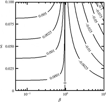
Figure 2. Variations of the pressure gradient correction
 $\mathit{Re}\,\text{d}p_{1}/\text{d}x$
in a channel with geometry defined by (2.8) as a function of the groove wavenumber
$\mathit{Re}\,\text{d}p_{1}/\text{d}x$
in a channel with geometry defined by (2.8) as a function of the groove wavenumber
 ${\it\beta}$
and the groove amplitude
${\it\beta}$
and the groove amplitude
 $S$
.
$S$
.
In the above, subscripts 0 and 1 denote the reference flow and the flow modifications, respectively. The governing equations for the flow modifications take the form
 $$\begin{eqnarray}\frac{\partial ^{2}u_{1}}{\partial y^{2}}+\frac{\partial ^{2}u_{1}}{\partial z^{2}}-\mathit{Re}\,\frac{\text{d}p_{1}}{\text{d}x}=0,\quad u_{0}(y_{L},z)+u_{1}(y_{L},z)=0,\quad u_{0}(1,z)+u_{1}(1,z)=0,\end{eqnarray}$$
 $$\begin{eqnarray}Q={\it\lambda}_{z}^{-1}\int _{z=0}^{z={\it\lambda}_{z}}\int _{y=y_{L}(z)}^{y=1}[u_{0}(y)+u_{1}(y,z)]\,\text{d}y\,\text{d}z=\frac{4}{3},\end{eqnarray}$$
and demonstrate that the character of the velocity field is independent of
 $\mathit{Re}$
. Solution of (2.6) has to be determined numerically due to geometric complexities. A spectral discretization method based on the Fourier and Chebyshev expansions is used (Mohammadi & Floryan Reference Mohammadi and Floryan2012; Moradi & Floryan Reference Moradi and Floryan2014). The solution is assumed to be in the form of a Fourier expansion in the
$\mathit{Re}$
. Solution of (2.6) has to be determined numerically due to geometric complexities. A spectral discretization method based on the Fourier and Chebyshev expansions is used (Mohammadi & Floryan Reference Mohammadi and Floryan2012; Moradi & Floryan Reference Moradi and Floryan2014). The solution is assumed to be in the form of a Fourier expansion in the
 $z$
-direction, i.e.
$z$
-direction, i.e.
 $$\begin{eqnarray}u_{1}(y,z)=\mathop{\sum }_{m=-\infty }^{m=+\infty }u_{1}^{(m)}(y)\text{e}^{\text{i}m{\it\beta}z},\end{eqnarray}$$
where
 $u_{1}^{(m)}=u_{1}^{(-m)\ast }$
expresses the reality condition. Chebyshev expansions are used for discretization of the modal functions
$u_{1}^{(m)}=u_{1}^{(-m)\ast }$
expresses the reality condition. Chebyshev expansions are used for discretization of the modal functions
 $u_{1}^{(m)}(y)$
. The Galerkin projection method is used to form a system of linear algebraic equations. The IBC concept (Szumbarski & Floryan Reference Szumbarski and Floryan1999; Mohammadi & Floryan Reference Mohammadi and Floryan2012) is used to enforce the boundary conditions. The IBC method relies on the use of a fixed regular computational domain extending in the
$u_{1}^{(m)}(y)$
. The Galerkin projection method is used to form a system of linear algebraic equations. The IBC concept (Szumbarski & Floryan Reference Szumbarski and Floryan1999; Mohammadi & Floryan Reference Mohammadi and Floryan2012) is used to enforce the boundary conditions. The IBC method relies on the use of a fixed regular computational domain extending in the
 $y$
-direction far enough so that it completely encloses the grooved channel, and imposition of the flow boundary conditions is carried out through specially constructed boundary relations using the tau concept (Canuto et al.
Reference Canuto, Hussaini, Quarteroni and Zang2006). The fixed volume flow rate constraint is discretized directly and the pressure gradient correction is determined simultaneously with the velocity field through the solution of a system consisting of the field equation, the boundary constraints and the volumetric flow rate constraint. Numerical parameters have been chosen through careful experimentation to guarantee at least six digits of accuracy. Certain cases were tested using the DT method.
$y$
-direction far enough so that it completely encloses the grooved channel, and imposition of the flow boundary conditions is carried out through specially constructed boundary relations using the tau concept (Canuto et al.
Reference Canuto, Hussaini, Quarteroni and Zang2006). The fixed volume flow rate constraint is discretized directly and the pressure gradient correction is determined simultaneously with the velocity field through the solution of a system consisting of the field equation, the boundary constraints and the volumetric flow rate constraint. Numerical parameters have been chosen through careful experimentation to guarantee at least six digits of accuracy. Certain cases were tested using the DT method.
The properties of the mean flow are illustrated for a groove geometry of the form
 $$\begin{eqnarray}y_{L}(z)=-1+S\cos ({\it\beta}z),\quad y_{U}=1,\end{eqnarray}$$
i.e. the lower wall is fitted with sinusoidal grooves. Figure 2 illustrates variations of the pressure gradient corrections as a function of
 ${\it\beta}$
and
${\it\beta}$
and
 $S$
, and demonstrates that grooves of sufficiently long wavelength reduce the pressure gradient required to drive the flow. The velocity distribution illustrated in figure 3(a) demonstrates the formation of a stream tube with elevated velocity in the widest channel opening. Figure 3(b) displays spanwise velocity variations in the middle of the channel and demonstrates that the stream tube exists for medium and long groove wavelengths but disappears for grooves with sufficiently short wavelengths. The latter effect is associated with the stream lift-up phenomenon and the apparent hydraulic wall thickening (Mohammadi & Floryan Reference Mohammadi and Floryan2013a
). The same figure demonstrates the appearance of inflection points in the spanwise velocity distributions; there are no inflection points in the wall-normal velocity distributions at any spanwise location. The vorticity field has just two non-zero components, i.e.
$S$
, and demonstrates that grooves of sufficiently long wavelength reduce the pressure gradient required to drive the flow. The velocity distribution illustrated in figure 3(a) demonstrates the formation of a stream tube with elevated velocity in the widest channel opening. Figure 3(b) displays spanwise velocity variations in the middle of the channel and demonstrates that the stream tube exists for medium and long groove wavelengths but disappears for grooves with sufficiently short wavelengths. The latter effect is associated with the stream lift-up phenomenon and the apparent hydraulic wall thickening (Mohammadi & Floryan Reference Mohammadi and Floryan2013a
). The same figure demonstrates the appearance of inflection points in the spanwise velocity distributions; there are no inflection points in the wall-normal velocity distributions at any spanwise location. The vorticity field has just two non-zero components, i.e.
 $$\begin{eqnarray}{\bf\omega}_{B}=({\it\xi}_{B},{\it\eta}_{B},{\it\phi}_{B})=(0,\partial u_{B}/\partial z,-\partial u_{B}/\partial y),\end{eqnarray}$$
with extrema of
 ${\it\eta}_{B}$
identifying locations of the spanwise inflection points (not shown). The flow can be viewed as consisting of sheets of constant
${\it\eta}_{B}$
identifying locations of the spanwise inflection points (not shown). The flow can be viewed as consisting of sheets of constant
 $z$
-vorticity in the case of the smooth channel; these sheets are deformed by the grooves, which, in addition, generate the
$z$
-vorticity in the case of the smooth channel; these sheets are deformed by the grooves, which, in addition, generate the
 $y$
-vorticity component. It is simple to show that the viscous dissipation function
$y$
-vorticity component. It is simple to show that the viscous dissipation function
 ${\it\Phi}_{B}$
, defined as
${\it\Phi}_{B}$
, defined as
 $$\begin{eqnarray}{\it\Phi}_{B}=\left(\frac{\partial u_{B}}{\partial y}\right)^{2}+\left(\frac{\partial u_{B}}{\partial z}\right)^{2},\end{eqnarray}$$
is strongest near the walls and negligible near the centre of the channel.

Figure 3. (a) Spatial distribution of the streamwise velocity component
 $u_{B}$
for flow through a channel with geometry defined by (2.8) with
$u_{B}$
for flow through a channel with geometry defined by (2.8) with
 $S=0.035$
and
$S=0.035$
and
 ${\it\beta}=0.7$
. (b) Spanwise variations of
${\it\beta}=0.7$
. (b) Spanwise variations of
 $u_{B}$
at
$u_{B}$
at
 $y=0$
for
$y=0$
for
 ${\it\beta}=0.1$
, 0.7 and 10.
${\it\beta}=0.1$
, 0.7 and 10.
3. Linear stability analysis
The drag-reducing abilities of the long-wavelength grooves can be utilized only if the flow remains laminar. It is therefore of interest to determine the maximum critical Reynolds numbers that guarantee the flow stability for all possible groove forms. We shall assume that the disturbance level is low and thus the asymptotic stability can predict the onset conditions for secondary states. A high level of disturbances requires analysis of the transient growth (Szumbarski & Floryan Reference Szumbarski and Floryan2006) as well as information about the initial structure of the disturbance field.
3.1. Problem formulation
The governing equations can be expressed in terms of the continuity and the vorticity transport equations of the form
 $$\begin{eqnarray}\displaystyle & \boldsymbol{{\rm\nabla}}\boldsymbol{\cdot }\boldsymbol{V}=0, & \displaystyle\end{eqnarray}$$
 $$\begin{eqnarray}\displaystyle & \displaystyle \frac{\partial {\bf\omega}}{\partial t}-({\bf\omega}\boldsymbol{\cdot }\boldsymbol{{\rm\nabla}})\boldsymbol{V}+(\boldsymbol{V}\boldsymbol{\cdot }\boldsymbol{{\rm\nabla}}){\bf\omega}-\frac{1}{\mathit{Re}}{\rm\nabla}^{2}{\bf\omega}=0, & \displaystyle\end{eqnarray}$$
 $\boldsymbol{V}$
and
$\boldsymbol{V}$
and
 ${\bf\omega}=\boldsymbol{{\rm\nabla}}\times \boldsymbol{V}$
are the velocity and vorticity vectors, respectively (Floryan Reference Floryan1997). The flow quantities are expressed as a superposition of the basic flow and three-dimensional disturbances, i.e.
${\bf\omega}=\boldsymbol{{\rm\nabla}}\times \boldsymbol{V}$
are the velocity and vorticity vectors, respectively (Floryan Reference Floryan1997). The flow quantities are expressed as a superposition of the basic flow and three-dimensional disturbances, i.e.  $$\begin{eqnarray}\boldsymbol{V}(x,y,z,t)=\boldsymbol{V}_{B}(y,z)+\boldsymbol{V}_{D}(x,y,z,t),\end{eqnarray}$$
 $$\begin{eqnarray}{\bf\omega}(x,y,z,t)={\bf\omega}_{B}(y,z)+{\bf\omega}_{D}(x,y,z,t).\end{eqnarray}$$
In the above, subscript
 $D$
denotes the disturbance field and
$D$
denotes the disturbance field and
 $\boldsymbol{V}_{D}=(u_{D},v_{D},w_{D})$
and
$\boldsymbol{V}_{D}=(u_{D},v_{D},w_{D})$
and
 ${\bf\omega}_{D}=({\it\xi}_{D},{\it\eta}_{D},{\it\phi}_{D})$
stand for the disturbance velocity and vorticity vectors, respectively. Substitution of (3.2) into (3.1), subtraction of the basic flow and linearization lead to the disturbance equations of the form
${\bf\omega}_{D}=({\it\xi}_{D},{\it\eta}_{D},{\it\phi}_{D})$
stand for the disturbance velocity and vorticity vectors, respectively. Substitution of (3.2) into (3.1), subtraction of the basic flow and linearization lead to the disturbance equations of the form
 $$\begin{eqnarray}\displaystyle & \displaystyle \frac{\partial u_{D}}{\partial x}+\frac{\partial v_{D}}{\partial y}+\frac{\partial w_{D}}{\partial z}=0, & \displaystyle\end{eqnarray}$$
 $$\begin{eqnarray}\displaystyle & & \displaystyle \frac{\partial {\it\xi}_{D}}{\partial t}-{\it\eta}_{B}\frac{\partial u_{D}}{\partial y}-\frac{\partial u_{B}}{\partial y}{\it\eta}_{D}-{\it\phi}_{B}\frac{\partial u_{D}}{\partial z}-\frac{\partial u_{B}}{\partial z}{\it\phi}_{D}\nonumber\\ \displaystyle & & \displaystyle \qquad +\,u_{B}\frac{\partial {\it\xi}_{D}}{\partial x}-\frac{1}{\mathit{Re}}\left(\frac{\partial ^{2}{\it\xi}_{D}}{\partial x^{2}}+\frac{\partial ^{2}{\it\xi}_{D}}{\partial y^{2}}+\frac{\partial ^{2}{\it\xi}_{D}}{\partial z^{2}}\right)=0,\end{eqnarray}$$
 $$\begin{eqnarray}\displaystyle & & \displaystyle \frac{\partial {\it\eta}_{D}}{\partial t}-{\it\eta}_{B}\frac{\partial v_{D}}{\partial y}-{\it\phi}_{B}\frac{\partial v_{D}}{\partial z}+u_{B}\frac{\partial {\it\eta}_{D}}{\partial x}+\frac{\partial {\it\eta}_{B}}{\partial y}v_{D}\nonumber\\ \displaystyle & & \displaystyle \qquad +\,\frac{\partial {\it\eta}_{B}}{\partial z}w_{D}-\frac{1}{\mathit{Re}}\left(\frac{\partial ^{2}{\it\eta}_{D}}{\partial x^{2}}+\frac{\partial ^{2}{\it\eta}_{D}}{\partial y^{2}}+\frac{\partial ^{2}{\it\eta}_{D}}{\partial z^{2}}\right)=0,\end{eqnarray}$$
 $$\begin{eqnarray}\displaystyle & & \displaystyle \frac{\partial {\it\phi}_{D}}{\partial t}-{\it\eta}_{B}\frac{\partial w_{D}}{\partial y}-{\it\phi}_{B}\frac{\partial w_{D}}{\partial z}+u_{B}\frac{\partial {\it\phi}_{D}}{\partial x}+\frac{\partial {\it\phi}_{B}}{\partial y}v_{D}\nonumber\\ \displaystyle & & \displaystyle \qquad +\,\frac{\partial {\it\phi}_{B}}{\partial z}w_{D}-\frac{1}{\mathit{Re}}\left(\frac{\partial ^{2}{\it\phi}_{D}}{\partial x^{2}}+\frac{\partial ^{2}{\it\phi}_{D}}{\partial y^{2}}+\frac{\partial ^{2}{\it\phi}_{D}}{\partial z^{2}}\right)=0,\end{eqnarray}$$
 $$\begin{eqnarray}\boldsymbol{V}_{D}(x,y_{L},z,t)=0,\quad \boldsymbol{V}_{D}(x,y_{U},z,t)=0.\end{eqnarray}$$
The coefficients appearing in (3.3b–d
) are functions of the (
 $y,z$
)-coordinates and therefore the solution can be written as
$y,z$
)-coordinates and therefore the solution can be written as
 $$\begin{eqnarray}\boldsymbol{V}_{D}(x,y,z,t)=\boldsymbol{G}_{D}(y,z)\text{e}^{\text{i}({\it\delta}x+{\it\mu}z-{\it\sigma}t)}+\text{c.c.},\end{eqnarray}$$
 $$\begin{eqnarray}{\bf\omega}_{D}(x,y,z,t)={\it\bf\Omega}_{D}(y,z)\text{e}^{\text{i}({\it\delta}x+{\it\mu}z-{\it\sigma}t)}+\text{c.c.},\end{eqnarray}$$
where
 ${\it\delta}$
and
${\it\delta}$
and
 ${\it\mu}$
denote the real wavenumbers in the
${\it\mu}$
denote the real wavenumbers in the
 $x$
- and
$x$
- and
 $z$
-directions, respectively,
$z$
-directions, respectively,
 ${\it\sigma}={\it\sigma}_{r}+\text{i}{\it\sigma}_{i}$
is the complex amplification rate,
${\it\sigma}={\it\sigma}_{r}+\text{i}{\it\sigma}_{i}$
is the complex amplification rate,
 ${\it\sigma}_{i}$
is the rate of growth of disturbances,
${\it\sigma}_{i}$
is the rate of growth of disturbances,
 ${\it\sigma}_{r}$
is the frequency of disturbances and c.c. refers to complex conjugates. The amplitude functions
${\it\sigma}_{r}$
is the frequency of disturbances and c.c. refers to complex conjugates. The amplitude functions
 $\boldsymbol{G}_{D}(y,z)$
and
$\boldsymbol{G}_{D}(y,z)$
and
 ${\it\bf\Omega}_{D}(y,z)$
are periodic functions of
${\it\bf\Omega}_{D}(y,z)$
are periodic functions of
 $z$
and thus can be expressed in terms of Fourier expansions of the form
$z$
and thus can be expressed in terms of Fourier expansions of the form
 $$\begin{eqnarray}\displaystyle & \displaystyle \boldsymbol{G}_{D}(y,z)=\mathop{\sum }_{n=-\infty }^{n=+\infty }[g_{u}^{(n)}(y),g_{v}^{(n)}(y),g_{w}^{(n)}(y)]\text{e}^{\text{i}n{\it\beta}z}+\text{c.c.}, & \displaystyle\end{eqnarray}$$
 $$\begin{eqnarray}\displaystyle & \displaystyle {\it\bf\Omega}_{D}(y,z)=\mathop{\sum }_{n=-\infty }^{n=+\infty }[g_{{\it\xi}}^{(n)}(y),g_{{\it\eta}}^{(n)}(y),g_{{\it\phi}}^{(n)}(y)]\text{e}^{\text{i}n{\it\beta}z}+\text{c.c.} & \displaystyle\end{eqnarray}$$
Substitution of (3.6) into (3.5) leads to the disturbance velocity and vorticity components of the form
 $$\begin{eqnarray}\displaystyle & \displaystyle \boldsymbol{V}_{D}(x,y,z,t)=\mathop{\sum }_{n=-\infty }^{n=+\infty }[g_{u}^{(n)}(y),g_{v}^{(n)}(y),g_{w}^{(n)}(y)]\text{e}^{\text{i}[{\it\delta}x+({\it\mu}+n{\it\beta})z-{\it\sigma}t]}+\text{c.c.}, & \displaystyle\end{eqnarray}$$
 $$\begin{eqnarray}\displaystyle & \displaystyle {\bf\omega}_{D}(x,y,z,t)=\mathop{\sum }_{n=-\infty }^{n=+\infty }[g_{{\it\xi}}^{(n)}(y),g_{{\it\eta}}^{(n)}(y),g_{{\it\phi}}^{(n)}(y)]\text{e}^{\text{i}[{\it\delta}x+({\it\mu}+n{\it\beta})z-{\it\sigma}t]}+\text{c.c.} & \displaystyle\end{eqnarray}$$
A system of linear homogeneous ordinary differential equations for
 $g_{v}^{(n)}(y)$
and
$g_{v}^{(n)}(y)$
and
 $g_{{\it\eta}}^{(n)}(y)$
is obtained by substituting (3.7) and (2.7) into (3.3) and separating Fourier modes. This system, after extensive rearrangement, takes the form
$g_{{\it\eta}}^{(n)}(y)$
is obtained by substituting (3.7) and (2.7) into (3.3) and separating Fourier modes. This system, after extensive rearrangement, takes the form
 $$\begin{eqnarray}\displaystyle & \displaystyle T^{(n)}(y)g_{v}^{(n)}(y)=\mathop{\sum }_{m=-\infty }^{m=+\infty }[A_{v}^{(n,m)}(y)g_{v}^{(n-m)}(y)+A_{{\it\eta}}^{(n,m)}(y)g_{{\it\eta}}^{(n-m)}(y)], & \displaystyle\end{eqnarray}$$
 $$\begin{eqnarray}\displaystyle & \displaystyle S^{(n)}(y)g_{{\it\eta}}^{(n)}(y)+C^{(n)}(y)g_{v}^{(n)}(y)=\mathop{\sum }_{m=-\infty }^{m=+\infty }[B_{v}^{(n,m)}(y)g_{v}^{(n-m)}(y)+B_{{\it\eta}}^{(n,m)}(y)g_{{\it\eta}}^{(n-m)}(y)],\qquad & \displaystyle\end{eqnarray}$$
 $-\infty <n<+\infty$
,
$-\infty <n<+\infty$
,  $$\begin{eqnarray}T^{(n)}(y)=\text{i}[-{\it\sigma}+{\it\delta}u_{0}(y)](\text{D}^{2}-k_{n}^{2})-\text{i}{\it\delta}\text{D}^{2}u_{0}(y)-\frac{1}{\mathit{Re}}(\text{D}^{2}-k_{n}^{2})^{2},\end{eqnarray}$$
 $$\begin{eqnarray}S^{(n)}(y)=\text{i}[-{\it\sigma}+{\it\delta}u_{0}(y)]-\frac{1}{\mathit{Re}}(\text{D}^{2}-k_{n}^{2}),\quad C^{(n)}(y)=\text{i}t_{n}\text{D}u_{0}(y),\end{eqnarray}$$
 $$\begin{eqnarray}\displaystyle A_{v}^{(n,m)}(y) & = & \displaystyle \text{i}{\it\delta}[k_{n}^{2}u_{1}^{(m)}(y)+\text{D}^{2}u_{1}^{(m)}(y)]\nonumber\\ \displaystyle & & \displaystyle -\,\frac{2\text{i}m{\it\beta}{\it\delta}t_{n-m}}{k_{n-m}^{2}}\text{D}u_{1}^{(m)}(y)\text{D}-\frac{\text{i}{\it\delta}}{k_{n-m}^{2}}(k_{n}^{2}-m^{2}{\it\beta}^{2})u_{1}^{(m)}(y)\text{D}^{2},\end{eqnarray}$$
 $$\begin{eqnarray}A_{{\it\eta}}^{(n,m)}(y)=-\frac{2\text{i}m{\it\beta}{\it\delta}^{2}}{k_{n-m}^{2}}[u_{1}^{(m)}(y)\text{D}+\text{D}u_{1}^{(m)}(y)],\end{eqnarray}$$
 $$\begin{eqnarray}B_{v}^{(n,m)}(y)=-\text{i}t_{n}\text{D}u_{1}^{(m)}(y)+\text{i}m{\it\beta}\left(1+\frac{m{\it\beta}t_{n-m}}{k_{n-m}^{2}}\right)u_{1}^{(m)}\text{D},\end{eqnarray}$$
 $$\begin{eqnarray}B_{{\it\eta}}^{(n,m)}(y)=-\text{i}{\it\delta}\left(1-\frac{m^{2}{\it\beta}^{2}}{k_{n-m}^{2}}\right)u_{1}^{(m)}(y),\end{eqnarray}$$
 $$\begin{eqnarray}k_{n}^{2}={\it\delta}^{2}+t_{n}^{2},\quad t_{n}={\it\mu}+n{\it\beta},\quad \text{D}^{q}=\text{d}^{q}/\text{d}y^{q}.\end{eqnarray}$$
The above formulation is analogous to the Bloch theory (Bloch Reference Bloch1929) for systems with spatially periodic coefficients and to the Floquet theory (Coddington & Levinson Reference Coddington and Levinson1965) for systems with time-periodic coefficients. The right-hand sides of (3.8) vanish in the limit of zero groove amplitude and the system reduces to an infinite set of uncoupled differential equations similar to those found in the case of stability of parallel flows. In analogy to such flows, we shall refer to the
 $T$
,
$T$
,
 $S$
and
$S$
and
 $C$
operators as the Orr–Sommerfeld, Squire and coupling operators, respectively (Floryan Reference Floryan1997). The eigenvalues of (3.8) have to be determined numerically, and the methods used in this work are briefly explained in the next section.
$C$
operators as the Orr–Sommerfeld, Squire and coupling operators, respectively (Floryan Reference Floryan1997). The eigenvalues of (3.8) have to be determined numerically, and the methods used in this work are briefly explained in the next section.
3.2. Numerical solution
The complete problem represents an eigenvalue problem for a system of ordinary differential equations (3.8) with homogeneous boundary conditions (3.4). Approximate solutions can be determined by truncating the Fourier expansions (3.7) at
 $N_{S}$
modes and thus solving (3.8) for
$N_{S}$
modes and thus solving (3.8) for
 $n=-N_{S},\dots ,-1,0,1,\dots ,N_{S}$
. The summations in (3.8) are truncated at
$n=-N_{S},\dots ,-1,0,1,\dots ,N_{S}$
. The summations in (3.8) are truncated at
 $N_{M}$
modes, where
$N_{M}$
modes, where
 $N_{M}\leqslant 2N_{S}$
denotes the number of Fourier modes used to represent the mean flow in the numerical solution. The modal functions are discretized using the Chebyshev expansions, and these expansions are truncated at Chebyshev polynomials of order
$N_{M}\leqslant 2N_{S}$
denotes the number of Fourier modes used to represent the mean flow in the numerical solution. The modal functions are discretized using the Chebyshev expansions, and these expansions are truncated at Chebyshev polynomials of order
 $N_{T}$
. The Galerkin projection method is used to construct a system of linear algebraic equations, and the boundary conditions are enforced using the IBC concept combined with the tau method (Szumbarski & Floryan Reference Szumbarski and Floryan1999; Floryan Reference Floryan2002; Moradi & Floryan Reference Moradi and Floryan2014). The DT method (Cabal et al.
Reference Cabal, Szumbarski and Floryan2002) provides an alternative if grooves with very large amplitudes are of interest.
$N_{T}$
. The Galerkin projection method is used to construct a system of linear algebraic equations, and the boundary conditions are enforced using the IBC concept combined with the tau method (Szumbarski & Floryan Reference Szumbarski and Floryan1999; Floryan Reference Floryan2002; Moradi & Floryan Reference Moradi and Floryan2014). The DT method (Cabal et al.
Reference Cabal, Szumbarski and Floryan2002) provides an alternative if grooves with very large amplitudes are of interest.
Several methods for tracing individual eigenvalues have been used, i.e. the shooting method combined with the Newton–Raphson procedure (Floryan Reference Floryan2002), the inverse iteration method (Floryan Reference Floryan2002) and the Arnoldi method (Saad Reference Saad2003). The inverse iteration method is preferred because of its good convergence properties but its applicability is limited to tracing of
 ${\it\sigma}$
, as it relies on complex arithmetic. The Newton–Raphson method requires careful tuning but is able to trace any combination of two real parameters. The Arnoldi method provides means for evaluation of segments of the spectra of large matrices such as those encountered in this analysis. The tracing of eigenvalues has been extended, if required, over several Brillouin zones (Bloch Reference Bloch1929) in the
${\it\sigma}$
, as it relies on complex arithmetic. The Newton–Raphson method requires careful tuning but is able to trace any combination of two real parameters. The Arnoldi method provides means for evaluation of segments of the spectra of large matrices such as those encountered in this analysis. The tracing of eigenvalues has been extended, if required, over several Brillouin zones (Bloch Reference Bloch1929) in the
 ${\it\mu}$
-direction in order to show how the leading eigenvalue is affected by the groove wavenumber.
${\it\mu}$
-direction in order to show how the leading eigenvalue is affected by the groove wavenumber.
4. Results
The flow in a smooth channel becomes unstable at
 $\mathit{Re}_{c}=5772$
, with two-dimensional TS waves with wavenumber
$\mathit{Re}_{c}=5772$
, with two-dimensional TS waves with wavenumber
 ${\it\delta}=1.02056$
travelling in the downstream direction playing the critical role (Orszag Reference Orszag1971). The instability has a subcritical character, and an increase of the level of disturbances can reduce the critical Reynolds number down to
${\it\delta}=1.02056$
travelling in the downstream direction playing the critical role (Orszag Reference Orszag1971). The instability has a subcritical character, and an increase of the level of disturbances can reduce the critical Reynolds number down to
 $\mathit{Re}_{c}\approx 2700$
(Herbert Reference Herbert1988). Numerous experiments demonstrate that the presence of distributed surface roughness changes the above scenario. Conditions when the transverse grooves (i.e. grooves transverse to the flow direction) with an arbitrary shape become hydraulically active, i.e. are able to create flow bifurcation, have been determined by Floryan (Reference Floryan2007), who identified changes in the critical conditions for the TS waves and demonstrated the growth of disturbances in the form of longitudinal vortices. The vortices are driven by centrifugal forces and are highly attenuated in the case of smooth walls. Predictions related to the TS waves have been confirmed experimentally (Asai & Floryan Reference Asai and Floryan2006). Analysis of the transient growth demonstrated that optimal disturbances have the form of streamwise vortices (Szumbarski & Floryan Reference Szumbarski and Floryan2006). Moradi & Floryan (Reference Moradi and Floryan2014) investigated the effects of longitudinal grooves (grooves parallel to the flow direction) and documented changes in the characteristics of the TS waves. They were able to demonstrate that short-wavelength grooves destabilize such waves while long-wavelength grooves stabilize them, when compared with their behaviour in a smooth channel. Below, we shall describe another class of disturbances whose growth is promoted by the longitudinal grooves; these disturbances are strongly attenuated in the smooth channel.
$\mathit{Re}_{c}\approx 2700$
(Herbert Reference Herbert1988). Numerous experiments demonstrate that the presence of distributed surface roughness changes the above scenario. Conditions when the transverse grooves (i.e. grooves transverse to the flow direction) with an arbitrary shape become hydraulically active, i.e. are able to create flow bifurcation, have been determined by Floryan (Reference Floryan2007), who identified changes in the critical conditions for the TS waves and demonstrated the growth of disturbances in the form of longitudinal vortices. The vortices are driven by centrifugal forces and are highly attenuated in the case of smooth walls. Predictions related to the TS waves have been confirmed experimentally (Asai & Floryan Reference Asai and Floryan2006). Analysis of the transient growth demonstrated that optimal disturbances have the form of streamwise vortices (Szumbarski & Floryan Reference Szumbarski and Floryan2006). Moradi & Floryan (Reference Moradi and Floryan2014) investigated the effects of longitudinal grooves (grooves parallel to the flow direction) and documented changes in the characteristics of the TS waves. They were able to demonstrate that short-wavelength grooves destabilize such waves while long-wavelength grooves stabilize them, when compared with their behaviour in a smooth channel. Below, we shall describe another class of disturbances whose growth is promoted by the longitudinal grooves; these disturbances are strongly attenuated in the smooth channel.

Figure 4. Disturbance spectrum for flow in a channel with geometry defined by (2.8) with
 ${\it\beta}=0.7$
and
${\it\beta}=0.7$
and
 $S=0.035$
for
$S=0.035$
for
 $\mathit{Re}=6000$
and disturbances with
$\mathit{Re}=6000$
and disturbances with
 ${\it\delta}=1.02$
and
${\it\delta}=1.02$
and
 ${\it\mu}=0$
computed using
${\it\mu}=0$
computed using
 $N_{S}=10$
Fourier modes and Chebyshev polynomials up to order
$N_{S}=10$
Fourier modes and Chebyshev polynomials up to order
 $N_{T}=250$
. Black crosses identify elements of the spectrum. The Orr–Sommerfeld spectrum for the smooth channel is given for comparison purposes and is identified using grey circles. The width of branch S is dictated by the number of Fourier modes used in the solution.
$N_{T}=250$
. Black crosses identify elements of the spectrum. The Orr–Sommerfeld spectrum for the smooth channel is given for comparison purposes and is identified using grey circles. The width of branch S is dictated by the number of Fourier modes used in the solution.
As the number of possible groove shapes is uncountable, we begin the discussion with grooves described by a single Fourier mode with the resulting channel geometry described by (2.8). This simplifies the discussion, as the number of geometric parameters is reduced to two, i.e. the groove wavenumber
 ${\it\beta}$
and the groove amplitude
${\it\beta}$
and the groove amplitude
 $S$
.
$S$
.
4.1. Sinusoidal grooves
We begin discussion by considering travelling wave disturbances, which connect to the classical TS waves in the limit of
 $S\rightarrow 0$
. The full disturbance spectrum for
$S\rightarrow 0$
. The full disturbance spectrum for
 $\mathit{Re}=6000$
,
$\mathit{Re}=6000$
,
 $S=0.035$
and
$S=0.035$
and
 ${\it\beta}=0.7$
for the ‘two-dimensional’ waves with
${\it\beta}=0.7$
for the ‘two-dimensional’ waves with
 ${\it\delta}=1.02$
and
${\it\delta}=1.02$
and
 ${\it\mu}=0$
is displayed in figure 4. The term ‘two-dimensional’ is given in quote marks, as disturbances are always three-dimensional owing to the groove-imposed modulations, but reduce to the purely two-dimensional form for
${\it\mu}=0$
is displayed in figure 4. The term ‘two-dimensional’ is given in quote marks, as disturbances are always three-dimensional owing to the groove-imposed modulations, but reduce to the purely two-dimensional form for
 $S\rightarrow 0$
. The dominant eigenvalue is located at the tip of branch A (wall modes; Mack Reference Mack1976) and its location is weakly affected by the grooves. Comparison of the disturbance velocity eigenfunctions for
$S\rightarrow 0$
. The dominant eigenvalue is located at the tip of branch A (wall modes; Mack Reference Mack1976) and its location is weakly affected by the grooves. Comparison of the disturbance velocity eigenfunctions for
 $S=0$
and
$S=0$
and
 $S\neq 0$
shows small differences in the
$S\neq 0$
shows small differences in the
 $x$
- and
$x$
- and
 $y$
-velocity components and the formation of wall layers with highly intense spanwise motions (figure 5). The results displayed in figure 6(a) demonstrate that this mode connects to the TS waves for
$y$
-velocity components and the formation of wall layers with highly intense spanwise motions (figure 5). The results displayed in figure 6(a) demonstrate that this mode connects to the TS waves for
 $S\rightarrow 0$
. The flow topology illustrated in figure 7 is very similar to that found in the smooth channel, i.e. it consists of a set of spanwise rolls propagating in the streamwise direction. The rolls are modified by the spanwise movements concentrated in the wall layers, with the fluid periodically flowing away from the corrugation peaks near the corrugated wall and towards the peaks at the opposite wall, with these directions reversed every quarter wavelength (see figure 8). Very strong spanwise movement in the wall layers occurs at the beginning of the disturbance wavelength (
$S\rightarrow 0$
. The flow topology illustrated in figure 7 is very similar to that found in the smooth channel, i.e. it consists of a set of spanwise rolls propagating in the streamwise direction. The rolls are modified by the spanwise movements concentrated in the wall layers, with the fluid periodically flowing away from the corrugation peaks near the corrugated wall and towards the peaks at the opposite wall, with these directions reversed every quarter wavelength (see figure 8). Very strong spanwise movement in the wall layers occurs at the beginning of the disturbance wavelength (
 $x=0$
, see figure 8
a), followed by a very strong vertical movement in the channel centre a quarter wavelength further downstream (
$x=0$
, see figure 8
a), followed by a very strong vertical movement in the channel centre a quarter wavelength further downstream (
 $x={\it\lambda}_{x}/4$
; see figure 8
b). The presence of grooves adds structures in the central part of the channel, which can be described as very weak vertical rolls (see figure 9
a); there is no trace of these structures in the wall layers (see figure 9
b).
$x={\it\lambda}_{x}/4$
; see figure 8
b). The presence of grooves adds structures in the central part of the channel, which can be described as very weak vertical rolls (see figure 9
a); there is no trace of these structures in the wall layers (see figure 9
b).

Figure 5. Disturbance velocity eigenfunctions (a)
 $g_{u}^{(n)}$
(
$g_{u}^{(n)}$
(
 $n=0$
, 1, 2), (b)
$n=0$
, 1, 2), (b)
 $g_{v}^{(n)}$
(
$g_{v}^{(n)}$
(
 $n=0,1,2$
) and (c)
$n=0,1,2$
) and (c)
 $g_{w}^{(n)}$
(
$g_{w}^{(n)}$
(
 $n=1,2,3$
) associated with the most unstable eigenvalue for
$n=1,2,3$
) associated with the most unstable eigenvalue for
 $\mathit{Re}=6000$
,
$\mathit{Re}=6000$
,
 $S=0.035$
,
$S=0.035$
,
 ${\it\beta}=0.7$
,
${\it\beta}=0.7$
,
 ${\it\delta}=1.02$
and
${\it\delta}=1.02$
and
 ${\it\mu}=0$
, normalized by the condition
${\it\mu}=0$
, normalized by the condition
 $\max _{0\leqslant y\leqslant 1}|g_{u}^{(0)}(y)|=1$
. The solid and dashed lines correspond to the real and imaginary parts, respectively. Eigenfunctions for the TS waves in a smooth channel are shown in (a) and (b) using grey lines.
$\max _{0\leqslant y\leqslant 1}|g_{u}^{(0)}(y)|=1$
. The solid and dashed lines correspond to the real and imaginary parts, respectively. Eigenfunctions for the TS waves in a smooth channel are shown in (a) and (b) using grey lines.

Figure 6. Variations of the growth rate
 ${\it\sigma}_{i}$
and the frequency
${\it\sigma}_{i}$
and the frequency
 ${\it\sigma}_{r}$
of the ‘two-dimensional’ disturbances (
${\it\sigma}_{r}$
of the ‘two-dimensional’ disturbances (
 ${\it\mu}=0$
) as a function of the groove amplitude
${\it\mu}=0$
) as a function of the groove amplitude
 $S$
for the groove geometry described by (2.8) with
$S$
for the groove geometry described by (2.8) with
 ${\it\beta}=0.7$
for the flow Reynolds number
${\it\beta}=0.7$
for the flow Reynolds number
 $\mathit{Re}=6000$
and disturbances with streamwise wavenumber
$\mathit{Re}=6000$
and disturbances with streamwise wavenumber
 ${\it\delta}=1.02$
(a) and
${\it\delta}=1.02$
(a) and
 ${\it\delta}=0.3$
(b). Dashed lines identify the imaginary and real parts of the most unstable TS waves with
${\it\delta}=0.3$
(b). Dashed lines identify the imaginary and real parts of the most unstable TS waves with
 ${\it\delta}=1.02$
in the smooth channel (a) and the least stable Squire mode with
${\it\delta}=1.02$
in the smooth channel (a) and the least stable Squire mode with
 ${\it\delta}=0.3$
in the smooth channel (b).
${\it\delta}=0.3$
in the smooth channel (b).

Figure 7. Disturbance velocity vectors in the (
 $x,y$
)-plane in the smooth channel (a) and in the corrugated channel at
$x,y$
)-plane in the smooth channel (a) and in the corrugated channel at
 $z={\it\lambda}_{z}/4$
(b) for the TS waves for the same conditions as in figure 5 and normalized by the condition
$z={\it\lambda}_{z}/4$
(b) for the TS waves for the same conditions as in figure 5 and normalized by the condition
 $\max _{y_{L}\leqslant y\leqslant 1,\,0\leqslant z\leqslant {\it\lambda}_{z}}|u_{D}(0,y,z,0)|=1$
.
$\max _{y_{L}\leqslant y\leqslant 1,\,0\leqslant z\leqslant {\it\lambda}_{z}}|u_{D}(0,y,z,0)|=1$
.


Figure 10 displays the spectrum for the same flow conditions and channel geometry but for a different class of disturbances, e.g. for
 ${\it\delta}=0.3$
and
${\it\delta}=0.3$
and
 ${\it\mu}=0$
. The unstable eigenvalue is located at the tip of branch P (centre modes) and its location is strongly affected by the groove amplitude. This mode connects to the Squire mode in the limit of
${\it\mu}=0$
. The unstable eigenvalue is located at the tip of branch P (centre modes) and its location is strongly affected by the groove amplitude. This mode connects to the Squire mode in the limit of
 $S\rightarrow 0$
as demonstrated in figure 6(b). The velocity eigenfunction for the limiting Squire mode is displayed in figure 11 and demonstrates that the fluid movement occurs only in the spanwise direction, resulting in the three-dimensionalization of the velocity field in a nominally two-dimensional flow even when the spanwise disturbance wavenumber
$S\rightarrow 0$
as demonstrated in figure 6(b). The velocity eigenfunction for the limiting Squire mode is displayed in figure 11 and demonstrates that the fluid movement occurs only in the spanwise direction, resulting in the three-dimensionalization of the velocity field in a nominally two-dimensional flow even when the spanwise disturbance wavenumber
 ${\it\mu}=0$
. Figure 11 also displays velocity eigenfunctions for the leading mode from the spectrum shown in figure 10 and demonstrates a significant change in the disturbance flow field. The
${\it\mu}=0$
. Figure 11 also displays velocity eigenfunctions for the leading mode from the spectrum shown in figure 10 and demonstrates a significant change in the disturbance flow field. The
 $x$
- and
$x$
- and
 $z$
-velocity components are
$z$
-velocity components are
 $O(1)$
while the
$O(1)$
while the
 $y$
-component is significantly smaller, suggesting that the disturbance motion retains a nearly planar character, i.e. it is confined mostly to the (
$y$
-component is significantly smaller, suggesting that the disturbance motion retains a nearly planar character, i.e. it is confined mostly to the (
 $x,z$
)-plane. The topology of the disturbance velocity field illustrated in figure 12 suggests that this field is made up of rows of counter-rotating rolls oriented across the channel and propagating in the streamwise direction. There are two rows of rolls per one groove wavelength, one centred at the widest channel opening and the other one centred at the narrowest opening, with the former one being stronger.
$x,z$
)-plane. The topology of the disturbance velocity field illustrated in figure 12 suggests that this field is made up of rows of counter-rotating rolls oriented across the channel and propagating in the streamwise direction. There are two rows of rolls per one groove wavelength, one centred at the widest channel opening and the other one centred at the narrowest opening, with the former one being stronger.

Figure 10. Disturbance spectrum for flow in a channel with geometry defined by (2.8) with
 ${\it\beta}=0.7$
and
${\it\beta}=0.7$
and
 $S=0.035$
for
$S=0.035$
for
 $\mathit{Re}=6000$
and disturbances with
$\mathit{Re}=6000$
and disturbances with
 ${\it\delta}=0.3$
and
${\it\delta}=0.3$
and
 ${\it\mu}=0$
computed using
${\it\mu}=0$
computed using
 $N_{S}=10$
Fourier modes and
$N_{S}=10$
Fourier modes and
 $N_{T}=250$
Chebyshev polynomials. Black crosses identify elements of the spectrum. The Squire spectrum for the smooth channel is given for comparison purposes and is identified using grey circles. The width of branch S is dictated by the number of Fourier modes used in the solution.
$N_{T}=250$
Chebyshev polynomials. Black crosses identify elements of the spectrum. The Squire spectrum for the smooth channel is given for comparison purposes and is identified using grey circles. The width of branch S is dictated by the number of Fourier modes used in the solution.
Figure 11. Disturbance velocity eigenfunctions (a)
 $g_{u}^{(n)}$
(
$g_{u}^{(n)}$
(
 $n=1$
, 2, 3), (b)
$n=1$
, 2, 3), (b)
 $g_{v}^{(n)}$
(
$g_{v}^{(n)}$
(
 $n=1$
, 2, 3) and (c)
$n=1$
, 2, 3) and (c)
 $g_{w}^{(n)}$
(
$g_{w}^{(n)}$
(
 $n=0$
, 1, 2) associated with the most unstable eigenvalue for
$n=0$
, 1, 2) associated with the most unstable eigenvalue for
 $\mathit{Re}=6000$
,
$\mathit{Re}=6000$
,
 $S=0.035$
,
$S=0.035$
,
 ${\it\beta}=0.7$
,
${\it\beta}=0.7$
,
 ${\it\delta}=0.3$
and
${\it\delta}=0.3$
and
 ${\it\mu}=0$
, normalized by the condition
${\it\mu}=0$
, normalized by the condition
 $\max _{0\leqslant y\leqslant 1}|g_{w}^{(0)}(y)|=1$
. The solid and dashed lines correspond to the real and imaginary parts, respectively. Eigenfunctions for the Squire mode in a smooth channel are shown in (c) using grey lines.
$\max _{0\leqslant y\leqslant 1}|g_{w}^{(0)}(y)|=1$
. The solid and dashed lines correspond to the real and imaginary parts, respectively. Eigenfunctions for the Squire mode in a smooth channel are shown in (c) using grey lines.

Figure 12. Disturbance velocity vectors in the (
 $y,z$
)-plane at
$y,z$
)-plane at
 $x=0$
(a) and at
$x=0$
(a) and at
 $x={\it\lambda}_{x}/4$
(b), in the (
$x={\it\lambda}_{x}/4$
(b), in the (
 $x,z$
)-plane at
$x,z$
)-plane at
 $y=0$
(c), and in the (
$y=0$
(c), and in the (
 $x,y$
)-plane at
$x,y$
)-plane at
 $z={\it\lambda}_{z}/4$
(d) for the new mode for the same conditions as in figure 11 and normalized by the condition
$z={\it\lambda}_{z}/4$
(d) for the new mode for the same conditions as in figure 11 and normalized by the condition
 $\max _{y_{L}\leqslant y\leqslant 1,\,0\leqslant z\leqslant {\it\lambda}_{z}}|u_{D}(0,y,z,0)|=1$
.
$\max _{y_{L}\leqslant y\leqslant 1,\,0\leqslant z\leqslant {\it\lambda}_{z}}|u_{D}(0,y,z,0)|=1$
.
We shall now address the question of the origin of the new instability. It is known that the TS instability is driven by shear and a sufficient increase of
 $\mathit{Re}$
will lead to its eventual stabilization. This process is illustrated in figure 13(a), displaying variations of the amplification rate
$\mathit{Re}$
will lead to its eventual stabilization. This process is illustrated in figure 13(a), displaying variations of the amplification rate
 ${\it\sigma}_{i}$
as a function of
${\it\sigma}_{i}$
as a function of
 ${\it\delta}$
for increasing
${\it\delta}$
for increasing
 $\mathit{Re}$
. The initial destabilization is followed by stabilization when
$\mathit{Re}$
. The initial destabilization is followed by stabilization when
 $\mathit{Re}$
becomes sufficiently large. Figure 13(b) displays the results of a similar study for the new mode and demonstrates that the amplification rate becomes
$\mathit{Re}$
becomes sufficiently large. Figure 13(b) displays the results of a similar study for the new mode and demonstrates that the amplification rate becomes
 $\mathit{Re}$
-independent once
$\mathit{Re}$
-independent once
 $\mathit{Re}$
becomes large enough. These results demonstrate that the instability is driven by an inviscid mechanism. It is simple to show that the mean flow vorticity has local extrema and thus the vorticity dynamics drives the instability through the so-called inflection point instability (Fjørtoft Reference Fjørtoft1950). Figure 14 displays the distribution of the mean flow
$\mathit{Re}$
becomes large enough. These results demonstrate that the instability is driven by an inviscid mechanism. It is simple to show that the mean flow vorticity has local extrema and thus the vorticity dynamics drives the instability through the so-called inflection point instability (Fjørtoft Reference Fjørtoft1950). Figure 14 displays the distribution of the mean flow
 $y$
-vorticity component, which can be viewed as a measure of the ‘driving force’, as well as the distribution of the dissipation function
$y$
-vorticity component, which can be viewed as a measure of the ‘driving force’, as well as the distribution of the dissipation function
 ${\it\Phi}_{B}$
, which can be viewed as a measure of the ‘opposing force’. Quote marks are used here to underline the qualitative character of these terms. The ‘driving force’ increases monotonically in the downward direction while the dissipation function is smallest around the channel mid-line, with the local minima in the widest and narrowest channel openings, and increases with distance away from the channel centre. The optimal conditions for the initiation of the instability are on both sides of the widest channel opening slightly below the channel mid-line, as this is where the ratio of the ‘driving’ and ‘opposing’ forces is the highest. Another argument explaining the location of the most intense instability motion can be made by looking at the spanwise variations of the local Reynolds number
${\it\Phi}_{B}$
, which can be viewed as a measure of the ‘opposing force’. Quote marks are used here to underline the qualitative character of these terms. The ‘driving force’ increases monotonically in the downward direction while the dissipation function is smallest around the channel mid-line, with the local minima in the widest and narrowest channel openings, and increases with distance away from the channel centre. The optimal conditions for the initiation of the instability are on both sides of the widest channel opening slightly below the channel mid-line, as this is where the ratio of the ‘driving’ and ‘opposing’ forces is the highest. Another argument explaining the location of the most intense instability motion can be made by looking at the spanwise variations of the local Reynolds number
 $\mathit{Re}_{loc}$
, which is based on the maximum velocity and the channel half-height at a given spanwise
$\mathit{Re}_{loc}$
, which is based on the maximum velocity and the channel half-height at a given spanwise
 $z$
-location, i.e.
$z$
-location, i.e.
 $$\begin{eqnarray}\mathit{Re}_{loc}=U_{max,loc}K_{loc}/{\it\nu}=\mathit{Re}\,u_{B,max}[1-S\cos ({\it\beta}z)/2].\end{eqnarray}$$
The variations of
 $\mathit{Re}_{loc}$
illustrated in figure 15 demonstrate that
$\mathit{Re}_{loc}$
illustrated in figure 15 demonstrate that
 $\mathit{Re}_{loc}$
is largest at the widest channel opening and suggests that this is where the balance between the inertial and viscous forces is most favourable for the instability.
$\mathit{Re}_{loc}$
is largest at the widest channel opening and suggests that this is where the balance between the inertial and viscous forces is most favourable for the instability.

Figure 13. Variations of the growth rate
 ${\it\sigma}_{i}$
of the ‘two-dimensional’ disturbances (
${\it\sigma}_{i}$
of the ‘two-dimensional’ disturbances (
 ${\it\mu}=0$
) as a function of the streamwise wavenumber
${\it\mu}=0$
) as a function of the streamwise wavenumber
 ${\it\delta}$
for flow in a channel with geometry described by (2.8) with
${\it\delta}$
for flow in a channel with geometry described by (2.8) with
 $S=0.035$
and
$S=0.035$
and
 ${\it\beta}=0.7$
for the TS waves (a) and the new mode (b).
${\it\beta}=0.7$
for the TS waves (a) and the new mode (b).

Figure 14. Distributions of the mean flow dissipation function
 ${\it\Phi}_{B}$
(black lines) and the mean flow normal vorticity component
${\it\Phi}_{B}$
(black lines) and the mean flow normal vorticity component
 ${\it\eta}_{B}=\partial u_{B}/\partial z$
(grey lines) in the middle of the channel with geometry described by (2.8) with
${\it\eta}_{B}=\partial u_{B}/\partial z$
(grey lines) in the middle of the channel with geometry described by (2.8) with
 $S=0.035$
and
$S=0.035$
and
 ${\it\beta}=0.7$
.
${\it\beta}=0.7$
.


The dominant eigenvalues identified through the analysis of the spectra shown in figures 4 and 10 determine the critical stability conditions. Their tracing through the parameter space provides the means for characterization of the instability. Figure 16(a,b) displays the neutral curves in the (
 $\mathit{Re},{\it\delta}$
)-plane for
$\mathit{Re},{\it\delta}$
)-plane for
 ${\it\beta}=1$
and typical groove amplitudes, and for
${\it\beta}=1$
and typical groove amplitudes, and for
 $S=0.05$
and typical groove wavenumbers. These results demonstrate the significantly different wavelengths of the most unstable TS waves and the most unstable new mode, as the critical wavenumber for the new mode is less than half of that for the TS waves. They also demonstrate a large sensitivity of the new mode, and the relative insensitivity of the TS waves, to the groove amplitude, as well as a rapid decrease of the critical Reynolds number
$S=0.05$
and typical groove wavenumbers. These results demonstrate the significantly different wavelengths of the most unstable TS waves and the most unstable new mode, as the critical wavenumber for the new mode is less than half of that for the TS waves. They also demonstrate a large sensitivity of the new mode, and the relative insensitivity of the TS waves, to the groove amplitude, as well as a rapid decrease of the critical Reynolds number
 $\mathit{Re}_{c}$
for the new mode as
$\mathit{Re}_{c}$
for the new mode as
 $S$
increases. The last observation is consistent with the results displayed in figure 6(b), which show a rapid increase of the amplification rate as
$S$
increases. The last observation is consistent with the results displayed in figure 6(b), which show a rapid increase of the amplification rate as
 $S$
increases.
$S$
increases.

Figure 16. Neutral curves in the (
 $\mathit{Re},{\it\delta}$
)-plane for the ‘two-dimensional’ disturbances (
$\mathit{Re},{\it\delta}$
)-plane for the ‘two-dimensional’ disturbances (
 ${\it\mu}=0$
) in a channel with geometry defined by (2.8). (a) Results for
${\it\mu}=0$
) in a channel with geometry defined by (2.8). (a) Results for
 ${\it\beta}=1$
and different
${\it\beta}=1$
and different
 $S$
. (b) Results for
$S$
. (b) Results for
 $S=0.05$
and different
$S=0.05$
and different
 ${\it\beta}$
. Solid and dotted lines correspond to the new mode and the TS waves, respectively.
${\it\beta}$
. Solid and dotted lines correspond to the new mode and the TS waves, respectively.
The effects of the groove wavenumber
 ${\it\beta}$
are illustrated in figure 17. It can be seen that the new mode can be induced by grooves with a finite range of
${\it\beta}$
are illustrated in figure 17. It can be seen that the new mode can be induced by grooves with a finite range of
 ${\it\beta}$
and that the range of ‘active’
${\it\beta}$
and that the range of ‘active’
 ${\it\beta}$
increases rapidly with an increase of both
${\it\beta}$
increases rapidly with an increase of both
 $S$
(a) and
$S$
(a) and
 $\mathit{Re}$
(b). The term ‘active’ refers to
$\mathit{Re}$
(b). The term ‘active’ refers to
 ${\it\beta}$
values that are able to induce this instability. An increase of
${\it\beta}$
values that are able to induce this instability. An increase of
 $\mathit{Re}$
corresponds to the reduction of the ‘opposing force’, while an increase of
$\mathit{Re}$
corresponds to the reduction of the ‘opposing force’, while an increase of
 $S$
corresponds to the increase of the ‘driving force’. The latter effect is illustrated in figure 18, which demonstrates a rapid increase of
$S$
corresponds to the increase of the ‘driving force’. The latter effect is illustrated in figure 18, which demonstrates a rapid increase of
 ${\it\eta}_{B}=\partial u_{B}/\partial z$
with an increase of
${\it\eta}_{B}=\partial u_{B}/\partial z$
with an increase of
 $S$
while, at the same time, the dissipation function remains nearly unchanged (not shown). The same figure also demonstrates a rapid decrease of
$S$
while, at the same time, the dissipation function remains nearly unchanged (not shown). The same figure also demonstrates a rapid decrease of
 ${\it\eta}_{B}=\partial u_{B}/\partial z$
for small and large
${\it\eta}_{B}=\partial u_{B}/\partial z$
for small and large
 ${\it\beta}$
values, which explains why such grooves are unable to support the new instability.
${\it\beta}$
values, which explains why such grooves are unable to support the new instability.

Figure 17. Neutral curves in the (
 ${\it\beta},{\it\delta}$
)-plane for the ‘two-dimensional’ disturbances (
${\it\beta},{\it\delta}$
)-plane for the ‘two-dimensional’ disturbances (
 ${\it\mu}=0$
) in a channel with geometry defined by (2.8). (a) Results for
${\it\mu}=0$
) in a channel with geometry defined by (2.8). (a) Results for
 $\mathit{Re}=7000$
and different
$\mathit{Re}=7000$
and different
 $S$
. (b) Results for
$S$
. (b) Results for
 $S=0.05$
and different
$S=0.05$
and different
 $\mathit{Re}$
. Solid and dotted lines correspond to the new mode and the TS waves, respectively.
$\mathit{Re}$
. Solid and dotted lines correspond to the new mode and the TS waves, respectively.

Figure 18. Variations of the maximum of the mean flow vertical vorticity component
 ${\it\eta}_{B}=\partial u_{B}/\partial z$
at
${\it\eta}_{B}=\partial u_{B}/\partial z$
at
 $y=0$
as a function of the groove wavenumber
$y=0$
as a function of the groove wavenumber
 ${\it\beta}$
in a channel with geometry defined by (2.8) with
${\it\beta}$
in a channel with geometry defined by (2.8) with
 $S=0.035$
.
$S=0.035$
.
So far, the discussion has only considered ‘two-dimensional’ waves, i.e.
 ${\it\mu}=0$
. The results displayed in figure 19 demonstrate that such waves play the critical role for the new mode, as the oblique waves are more attenuated. A similar conclusion for the TS waves has been reported by Moradi & Floryan (Reference Moradi and Floryan2014).
${\it\mu}=0$
. The results displayed in figure 19 demonstrate that such waves play the critical role for the new mode, as the oblique waves are more attenuated. A similar conclusion for the TS waves has been reported by Moradi & Floryan (Reference Moradi and Floryan2014).

Figure 19. Variations of the critical Reynolds number
 $\mathit{Re}_{c}$
for disturbances with the wavevector
$\mathit{Re}_{c}$
for disturbances with the wavevector
 $\boldsymbol{q}=({\it\delta},{\it\mu})$
as a function of its inclination angle
$\boldsymbol{q}=({\it\delta},{\it\mu})$
as a function of its inclination angle
 ${\it\theta}=\pm \text{tan}^{-1}({\it\mu}/{\it\delta})$
for the groove geometry described by (2.8) with
${\it\theta}=\pm \text{tan}^{-1}({\it\mu}/{\it\delta})$
for the groove geometry described by (2.8) with
 $S=0.05$
. Results correspond to the new mode with
$S=0.05$
. Results correspond to the new mode with
 $|\boldsymbol{q}|=({\it\delta}^{2}+{\it\mu}^{2})^{1/2}=0.3$
(black lines) and
$|\boldsymbol{q}|=({\it\delta}^{2}+{\it\mu}^{2})^{1/2}=0.3$
(black lines) and
 $|\boldsymbol{q}|=0.32$
(grey lines).
$|\boldsymbol{q}|=0.32$
(grey lines).
Figure 20 displays variations of the critical Reynolds number
 $\mathit{Re}_{c}$
as a function of the groove geometry, i.e.
$\mathit{Re}_{c}$
as a function of the groove geometry, i.e.
 ${\it\beta}$
and
${\it\beta}$
and
 $S$
, for the TS waves and for the new mode. The range of the unstable
$S$
, for the TS waves and for the new mode. The range of the unstable
 ${\it\beta}$
values for the new mode is clearly delineated together with the remarkable decrease of
${\it\beta}$
values for the new mode is clearly delineated together with the remarkable decrease of
 $\mathit{Re}_{c}$
when
$\mathit{Re}_{c}$
when
 $S$
increases. Variations of
$S$
increases. Variations of
 $\mathit{Re}_{c}$
for the TS waves can be viewed as marginal when compared with variations of
$\mathit{Re}_{c}$
for the TS waves can be viewed as marginal when compared with variations of
 $\mathit{Re}_{c}$
for the new mode. Figure 21 provides a zoom-in on the range of parameters where the new mode plays the critical role and, at the same time, expands the range of
$\mathit{Re}_{c}$
for the new mode. Figure 21 provides a zoom-in on the range of parameters where the new mode plays the critical role and, at the same time, expands the range of
 $S$
covered by the analysis; it provides detailed information about the critical Reynolds number
$S$
covered by the analysis; it provides detailed information about the critical Reynolds number
 $\mathit{Re}_{c}$
, the critical wavenumber
$\mathit{Re}_{c}$
, the critical wavenumber
 ${\it\delta}_{c}$
, the critical frequency
${\it\delta}_{c}$
, the critical frequency
 ${\it\sigma}_{r,c}$
and the critical phase speed
${\it\sigma}_{r,c}$
and the critical phase speed
 $c_{c}={\it\sigma}_{r,c}/{\it\delta}_{c}$
. It can be seen that
$c_{c}={\it\sigma}_{r,c}/{\it\delta}_{c}$
. It can be seen that
 $\mathit{Re}_{c}$
can be reduced down to
$\mathit{Re}_{c}$
can be reduced down to
 $\mathit{Re}_{c}<750$
for
$\mathit{Re}_{c}<750$
for
 $S=0.1$
. The range of unstable
$S=0.1$
. The range of unstable
 ${\it\beta}$
values has a rather steep, weakly
${\it\beta}$
values has a rather steep, weakly
 $S$
-dependent bound on the side of large
$S$
-dependent bound on the side of large
 ${\it\beta}$
, while it keeps expanding on the side of small
${\it\beta}$
, while it keeps expanding on the side of small
 ${\it\beta}$
as
${\it\beta}$
as
 $S$
increases. The critical wavenumber
$S$
increases. The critical wavenumber
 ${\it\delta}_{c}$
changes from
${\it\delta}_{c}$
changes from
 ${\sim}1$
for large
${\sim}1$
for large
 ${\it\beta}$
to
${\it\beta}$
to
 ${\sim}0.025$
for small
${\sim}0.025$
for small
 ${\it\beta}$
for the new mode while
${\it\beta}$
for the new mode while
 ${\it\delta}_{c}$
for the TS waves changes marginally. The critical frequency for the new mode changes from
${\it\delta}_{c}$
for the TS waves changes marginally. The critical frequency for the new mode changes from
 ${\sim}1$
for large
${\sim}1$
for large
 ${\it\beta}$
to
${\it\beta}$
to
 ${\sim}0.025$
for small
${\sim}0.025$
for small
 ${\it\beta}$
, while it remains nearly constant for the TS waves. The critical phase speed remains nearly constant at
${\it\beta}$
, while it remains nearly constant for the TS waves. The critical phase speed remains nearly constant at
 $c_{c}\approx 1$
for the new mode and at
$c_{c}\approx 1$
for the new mode and at
 $c_{c}\approx 0.26$
for the TS waves. In summary, at the onset one can observe the new mode with wavelength varying widely depending on the groove wavenumber but with a phase speed that is nearly always the same and approximately four times greater than the TS wave phase speed.
$c_{c}\approx 0.26$
for the TS waves. In summary, at the onset one can observe the new mode with wavelength varying widely depending on the groove wavenumber but with a phase speed that is nearly always the same and approximately four times greater than the TS wave phase speed.

Figure 20. Variations of the critical Reynolds number
 $\mathit{Re}_{c}$
as a function of the groove wavenumber
$\mathit{Re}_{c}$
as a function of the groove wavenumber
 ${\it\beta}$
and the groove amplitude
${\it\beta}$
and the groove amplitude
 $S$
in a channel with geometry defined by (2.8). Solid and dotted lines correspond to the ‘two-dimensional’ new mode (
$S$
in a channel with geometry defined by (2.8). Solid and dotted lines correspond to the ‘two-dimensional’ new mode (
 ${\it\mu}=0$
) and the two-dimensional TS waves (
${\it\mu}=0$
) and the two-dimensional TS waves (
 ${\it\mu}=0$
), respectively. The thick line separates zones where each mode plays the critical role. The zoom-in on the range of
${\it\mu}=0$
), respectively. The thick line separates zones where each mode plays the critical role. The zoom-in on the range of
 ${\it\beta}$
where the new mode determines the critical conditions together with an extension to larger values of
${\it\beta}$
where the new mode determines the critical conditions together with an extension to larger values of
 $S$
is given in figure 21.
$S$
is given in figure 21.

Figure 21. Variations of the critical stability parameters as a function of the groove wavenumber
 ${\it\beta}$
and the groove amplitude
${\it\beta}$
and the groove amplitude
 $S$
. Other conditions are as in figure 20. Variations of the critical Reynolds number
$S$
. Other conditions are as in figure 20. Variations of the critical Reynolds number
 $\mathit{Re}_{c}$
, the critical wavenumber
$\mathit{Re}_{c}$
, the critical wavenumber
 ${\it\delta}_{c}$
, the critical frequency
${\it\delta}_{c}$
, the critical frequency
 ${\it\sigma}_{r,c}$
and the critical phase speed
${\it\sigma}_{r,c}$
and the critical phase speed
 $c_{c}={\it\sigma}_{r,c}/{\it\delta}_{c}$
are displayed in panels (a)–(d), respectively.
$c_{c}={\it\sigma}_{r,c}/{\it\delta}_{c}$
are displayed in panels (a)–(d), respectively.
The reader may note that
 ${\it\beta}$
and
${\it\beta}$
and
 ${\it\delta}_{c}$
for the new mode satisfy the relation
${\it\delta}_{c}$
for the new mode satisfy the relation
 ${\it\delta}_{c}\approx {\it\beta}/2$
(see figure 21
b), which suggests that a parametric resonance is contributing to the instability. One can look at the grooves as one-dimensional spatially distributed forcing imposed on the flow and characterized by the wavevector (
${\it\delta}_{c}\approx {\it\beta}/2$
(see figure 21
b), which suggests that a parametric resonance is contributing to the instability. One can look at the grooves as one-dimensional spatially distributed forcing imposed on the flow and characterized by the wavevector (
 $0,{\it\beta}$
). Studies of simple model problems involving such forcing demonstrate that the dynamical system may exhibit wavenumber locking and responses that extend into two spatial dimensions, i.e. the system response may have a component in the direction orthogonal to the forcing wavevector (Manor, Hagberg & Meron Reference Manor, Hagberg and Meron2008, Reference Manor, Hagberg and Meron2009). Analysis of natural convection in a horizontal layer subject to one-dimensional spatial temperature modulations demonstrates that the system response is driven by a combination of the buoyancy-driven instability and the spatial parametric resonance, with each mechanism dominating over a different range of forcing wavelengths and the wavenumber locking between the forcing and the system response observed in the latter case (Hossain & Floryan Reference Hossain and Floryan2013). The forcing reduces the system symmetry to translational symmetry. Addition of a pressure-gradient-driven flow further affects the symmetry, with the system response showing preference for the flow direction (Hossain & Floryan Reference Hossain and Floryan2015). Such a system still exhibits characteristics associated with the spatial parametric resonance if the flow Reynolds number is small enough and the forcing is strong enough. Shear layers always have a preferred direction, e.g. the flow direction, and thus the effect of parametric resonance may be difficult to identify. The analysis is further complicated by the simultaneous appearance of shear, vorticity (inflection point mechanism) and centrifugal instability mechanisms. Floryan (Reference Floryan1997) studied pressure-gradient-driven channel flow modified by forcing in the form of streamwise suction or blowing and demonstrated that one possible response involves the formation of streamwise vortices, i.e. structures characterized by a wavevector with a component orthogonal to the forcing wavevector. Forcing generated by the transverse surface corrugations has led to similar conclusions for the pressure-gradient-driven flows as well as for the kinematically driven flows (Floryan Reference Floryan2002, Reference Floryan2007). The system response to forcing in the form of longitudinal grooves furthermore underscores the importance of the spatial parametric resonance.
$0,{\it\beta}$
). Studies of simple model problems involving such forcing demonstrate that the dynamical system may exhibit wavenumber locking and responses that extend into two spatial dimensions, i.e. the system response may have a component in the direction orthogonal to the forcing wavevector (Manor, Hagberg & Meron Reference Manor, Hagberg and Meron2008, Reference Manor, Hagberg and Meron2009). Analysis of natural convection in a horizontal layer subject to one-dimensional spatial temperature modulations demonstrates that the system response is driven by a combination of the buoyancy-driven instability and the spatial parametric resonance, with each mechanism dominating over a different range of forcing wavelengths and the wavenumber locking between the forcing and the system response observed in the latter case (Hossain & Floryan Reference Hossain and Floryan2013). The forcing reduces the system symmetry to translational symmetry. Addition of a pressure-gradient-driven flow further affects the symmetry, with the system response showing preference for the flow direction (Hossain & Floryan Reference Hossain and Floryan2015). Such a system still exhibits characteristics associated with the spatial parametric resonance if the flow Reynolds number is small enough and the forcing is strong enough. Shear layers always have a preferred direction, e.g. the flow direction, and thus the effect of parametric resonance may be difficult to identify. The analysis is further complicated by the simultaneous appearance of shear, vorticity (inflection point mechanism) and centrifugal instability mechanisms. Floryan (Reference Floryan1997) studied pressure-gradient-driven channel flow modified by forcing in the form of streamwise suction or blowing and demonstrated that one possible response involves the formation of streamwise vortices, i.e. structures characterized by a wavevector with a component orthogonal to the forcing wavevector. Forcing generated by the transverse surface corrugations has led to similar conclusions for the pressure-gradient-driven flows as well as for the kinematically driven flows (Floryan Reference Floryan2002, Reference Floryan2007). The system response to forcing in the form of longitudinal grooves furthermore underscores the importance of the spatial parametric resonance.
The results presented in figures 20 and 21 provide the basis for the identification of conditions that guarantee that the flow remains laminar in the presence of grooves, i.e. when the grooved surface behaves as a hydraulically smooth surface. Here we shall use the definition proposed by Floryan (Reference Floryan2007), which states that the corrugated wall can be viewed as hydraulically smooth as long as it is unable to create system bifurcation. It is convenient to introduce the global critical Reynolds number defined as
 $$\begin{eqnarray}\mathit{Re}_{c,g}=\min _{\begin{array}{@{}c@{}}{\it\beta}\\ (S\,=\,\text{const.})\end{array}}(\mathit{Re}_{c}),\end{eqnarray}$$
i.e. it is defined as the minimum of
 $\mathit{Re}_{c}$
over all groove wavenumbers for a given groove amplitude for a particular instability mode. Figure 22 displays variations of
$\mathit{Re}_{c}$
over all groove wavenumbers for a given groove amplitude for a particular instability mode. Figure 22 displays variations of
 $\mathit{Re}_{c,g}$
as a function of
$\mathit{Re}_{c,g}$
as a function of
 $S$
for the TS waves and for the new instability mode. The zone attached to the bottom left corner identifies conditions when the flow remains stable regardless of the spatial distributions of the grooves. When
$S$
for the TS waves and for the new instability mode. The zone attached to the bottom left corner identifies conditions when the flow remains stable regardless of the spatial distributions of the grooves. When
 $S<0.02$
, increase of
$S<0.02$
, increase of
 $\mathit{Re}$
will eventually lead to the onset of the TS wave instability and the corresponding conditions define the travelling wave limitation. When
$\mathit{Re}$
will eventually lead to the onset of the TS wave instability and the corresponding conditions define the travelling wave limitation. When
 $S>0.02$
, increase of
$S>0.02$
, increase of
 $\mathit{Re}$
will eventually activate the new mode and the corresponding conditions define the new mode limitation. The latter curve can be approximated as
$\mathit{Re}$
will eventually activate the new mode and the corresponding conditions define the new mode limitation. The latter curve can be approximated as
 $\mathit{Re}_{c,g}=4.505S^{-1.925}$
and it defines the upper limit of
$\mathit{Re}_{c,g}=4.505S^{-1.925}$
and it defines the upper limit of
 $S$
that guarantees flow stability. Conditions below the limiting curves guarantee flow stability for any groove distributions and thus walls with such grooves can be viewed as hydraulically smooth. The reader may note that not every groove distribution corresponding to the conditions above these curves must lead to flow instability.
$S$
that guarantees flow stability. Conditions below the limiting curves guarantee flow stability for any groove distributions and thus walls with such grooves can be viewed as hydraulically smooth. The reader may note that not every groove distribution corresponding to the conditions above these curves must lead to flow instability.

Figure 22. Variations of the global critical Reynolds number
 $\mathit{Re}_{c,g}$
as a function of the groove amplitude
$\mathit{Re}_{c,g}$
as a function of the groove amplitude
 $S$
for flow through a channel fitted with grooves of different shapes. Solid grey lines correspond to sinusoidal grooves defined by (2.8). Black dashed, dotted, solid and dash-dotted lines correspond to triangular grooves with
$S$
for flow through a channel fitted with grooves of different shapes. Solid grey lines correspond to sinusoidal grooves defined by (2.8). Black dashed, dotted, solid and dash-dotted lines correspond to triangular grooves with
 $a_{1}=b_{1}={\it\lambda}/2$
and
$a_{1}=b_{1}={\it\lambda}/2$
and
 $d_{1}=0$
, universal trapezoidal grooves with
$d_{1}=0$
, universal trapezoidal grooves with
 $a_{2}=b_{2}={\it\lambda}/8$
and
$a_{2}=b_{2}={\it\lambda}/8$
and
 $c_{2}=d_{2}=3{\it\lambda}/8$
, rectangular grooves with
$c_{2}=d_{2}=3{\it\lambda}/8$
, rectangular grooves with
 $c_{3}=d_{3}={\it\lambda}/2$
and circular-segment grooves with
$c_{3}=d_{3}={\it\lambda}/2$
and circular-segment grooves with
 $c_{4}=d_{4}={\it\lambda}/2$
, respectively (see figure 23 for definitions of geometric parameters). Correlation for the new instability mode for the most dangerous shape, i.e. the rectangular grooves, has the form
$c_{4}=d_{4}={\it\lambda}/2$
, respectively (see figure 23 for definitions of geometric parameters). Correlation for the new instability mode for the most dangerous shape, i.e. the rectangular grooves, has the form
 $\mathit{Re}_{c,g}=4.505S^{-1.925}$
.
$\mathit{Re}_{c,g}=4.505S^{-1.925}$
.
4.2. Grooves with arbitrary shapes
The above discussion was focused on grooves with shapes described by a single Fourier mode, i.e. (2.8). We shall now enquire how the new instability mode is affected by changes in the groove shape. It has been shown by Floryan (Reference Floryan2007) in the analysis of the stability of channel flow modified by transverse grooves, and by Moradi & Floryan (Reference Moradi and Floryan2014) in the analysis of the stability of the TS mode in a channel with longitudinal grooves, that groove shapes can be replaced with an acceptable accuracy by the leading mode from the Fourier expansion describing their geometry. These conclusions form the basis of the ROG model. It remains to be shown if the ROG model remains valid for the new mode. Figure 23 describes four general shapes used in the analysis, including rectangular grooves. The Fourier representation of the latter shape suffers from the Gibbs phenomenon, which has been controlled using a filtering technique based on the ‘raised cosine’ method (Canuto et al. Reference Canuto, Hussaini, Quarteroni and Zang2006). Figure 24 displays the neutral curves for the test grooves with their shapes replaced by a gradually increasing number of Fourier modes from Fourier expansions representing their shapes. It can be seen that the computed critical Reynolds numbers rapidly converge as the number of Fourier modes used for the geometry description increases. These results demonstrate that the ROG model can indeed be used in the analysis of the new mode and thus the results described in § 4.1 can be used to estimate the stability characteristics of arbitrary grooves with an acceptable accuracy.

Figure 23. Groove shapes used in this study: (a) triangular grooves, (b) trapezoidal grooves, (c) rectangular grooves, and (d) circular-segment grooves with
 $c_{4}\geqslant 4S$
and
$c_{4}\geqslant 4S$
and
 $R=c_{4}^{2}/(16S)+S$
.
$R=c_{4}^{2}/(16S)+S$
.

Figure 24. The neutral curves in the (
 $\mathit{Re},{\it\delta}$
)-plane for grooves with amplitude
$\mathit{Re},{\it\delta}$
)-plane for grooves with amplitude
 $S=0.05$
and wavenumber
$S=0.05$
and wavenumber
 ${\it\beta}=1$
. Dashed, dotted, solid and dash-dotted lines correspond to triangular grooves with
${\it\beta}=1$
. Dashed, dotted, solid and dash-dotted lines correspond to triangular grooves with
 $a_{1}=b_{1}={\it\lambda}/3$
,
$a_{1}=b_{1}={\it\lambda}/3$
,
 $d_{1}={\it\lambda}/3$
, trapezoidal grooves with
$d_{1}={\it\lambda}/3$
, trapezoidal grooves with
 $a_{2}=b_{2}={\it\lambda}/6$
,
$a_{2}=b_{2}={\it\lambda}/6$
,
 $c_{2}=d_{2}={\it\lambda}/3$
, rectangular grooves with
$c_{2}=d_{2}={\it\lambda}/3$
, rectangular grooves with
 $c_{3}=2{\it\lambda}/3$
,
$c_{3}=2{\it\lambda}/3$
,
 $d_{3}={\it\lambda}/3$
, and circular-segment grooves with
$d_{3}={\it\lambda}/3$
, and circular-segment grooves with
 $c_{4}=2{\it\lambda}/3$
,
$c_{4}=2{\it\lambda}/3$
,
 $d_{4}={\it\lambda}/3$
, respectively (see figure 23 for notation). (b) An enlargement of the box shown in (a). All grooves were represented in the analysis using one, three and five leading Fourier modes taken from the Fourier expansions describing their geometry.
$d_{4}={\it\lambda}/3$
, respectively (see figure 23 for notation). (b) An enlargement of the box shown in (a). All grooves were represented in the analysis using one, three and five leading Fourier modes taken from the Fourier expansions describing their geometry.
Figure 22 illustrates the variations of
 $\mathit{Re}_{c,g}$
for all these grooves. It can be seen that the TS wave limitation is little affected by changes of the groove shape. The curve defining the new mode limitations shifts as a function of the groove shape but the difference between the critical Reynolds number for the actual groove and for its reduced geometry representation remains below 10 %. Rectangular grooves appear to be the most effective in initiating the new instability mode, and thus one can define the parameter range where the grooved surface behaves as a hydraulically smooth surface using results for this particular shape.
$\mathit{Re}_{c,g}$
for all these grooves. It can be seen that the TS wave limitation is little affected by changes of the groove shape. The curve defining the new mode limitations shifts as a function of the groove shape but the difference between the critical Reynolds number for the actual groove and for its reduced geometry representation remains below 10 %. Rectangular grooves appear to be the most effective in initiating the new instability mode, and thus one can define the parameter range where the grooved surface behaves as a hydraulically smooth surface using results for this particular shape.

Figure 25. The neutral curves in the (
 $\mathit{Re},{\it\delta}$
)-plane for channels fitted with the optimal equal-depth grooves. Groove geometry is represented by the universal trapezoid with
$\mathit{Re},{\it\delta}$
)-plane for channels fitted with the optimal equal-depth grooves. Groove geometry is represented by the universal trapezoid with
 $a_{2}=b_{2}={\it\lambda}/8$
,
$a_{2}=b_{2}={\it\lambda}/8$
,
 $c_{2}=d_{2}=3{\it\lambda}/8$
and
$c_{2}=d_{2}=3{\it\lambda}/8$
and
 ${\it\beta}=0.7$
(see figure 23
b for notation). Results for sinusoidal grooves are given for reference (dotted lines). (b) An enlargement of the box shown in (a).
${\it\beta}=0.7$
(see figure 23
b for notation). Results for sinusoidal grooves are given for reference (dotted lines). (b) An enlargement of the box shown in (a).
4.3. Optimal grooves
The stability characteristics of the optimal grooves are of interest, as such grooves provide the largest possible drag reduction (Mohammadi & Floryan Reference Mohammadi and Floryan2013b ). The shapes of such grooves depend on the type of constraints. The channel geometry used for analysis is expressed as
 $$\begin{eqnarray}y_{L}(z)=-1+\mathop{\sum }_{m=-N_{A}}^{m=N_{A}}H_{L}^{(m)}\text{e}^{\text{i}m{\it\beta}z},\quad y_{U}(z)=1,\end{eqnarray}$$
and the groove height (
 $S_{L,max}$
) and depth (
$S_{L,max}$
) and depth (
 $S_{L,min}$
) are subject to constraints of the form
$S_{L,min}$
) are subject to constraints of the form
 $$\begin{eqnarray}S_{L,max}=\max \left(\mathop{\sum }_{m=-N_{A}}^{m=N_{A}}H_{L}^{(m)}\text{e}^{\text{i}m{\it\beta}z}\right),\quad S_{L,min}=-\text{min}\left(\mathop{\sum }_{m=-N_{A}}^{m=N_{A}}H_{L}^{(m)}\text{e}^{\text{i}m{\it\beta}z}\right).\end{eqnarray}$$
In the case of equal-depth grooves,
 $S_{L,max}=S_{L,min}=S$
. In the case of unequal-depth grooves, the height is set by (4.4a,b
) while the depth is determined by the optimization process (Mohammadi & Floryan Reference Mohammadi and Floryan2013b
). The shape of the optimal, equal-depth grooves can be well approximated by a universal trapezoid with
$S_{L,max}=S_{L,min}=S$
. In the case of unequal-depth grooves, the height is set by (4.4a,b
) while the depth is determined by the optimization process (Mohammadi & Floryan Reference Mohammadi and Floryan2013b
). The shape of the optimal, equal-depth grooves can be well approximated by a universal trapezoid with
 $a_{2}=b_{2}={\it\lambda}/8$
and
$a_{2}=b_{2}={\it\lambda}/8$
and
 $c_{2}=d_{2}=3{\it\lambda}/8$
(figure 23
b). The neutral stability curves for such grooves displayed in figure 25 demonstrate a significant loss of stability when compared with the simple sinusoidal grooves. The shapes of the unequal-depth grooves are illustrated in figure 26(a). If the
$c_{2}=d_{2}=3{\it\lambda}/8$
(figure 23
b). The neutral stability curves for such grooves displayed in figure 25 demonstrate a significant loss of stability when compared with the simple sinusoidal grooves. The shapes of the unequal-depth grooves are illustrated in figure 26(a). If the
 $y$
-coordinate is rescaled using the peak-to-bottom distance as the length scale
$y$
-coordinate is rescaled using the peak-to-bottom distance as the length scale
 $\bar{y}_{L}=(y_{L}+1-S_{L,max})/(S_{L,min}+S_{L,max})$
, and the
$\bar{y}_{L}=(y_{L}+1-S_{L,max})/(S_{L,min}+S_{L,max})$
, and the
 $z$
-coordinate is rescaled using the groove width at half-height
$z$
-coordinate is rescaled using the groove width at half-height
 $W_{half}$
as the length scale
$W_{half}$
as the length scale
 $\bar{z}=(z-z_{0})/W_{half}$
, the groove shape can be approximated using a Gaussian function of the form
$\bar{z}=(z-z_{0})/W_{half}$
, the groove shape can be approximated using a Gaussian function of the form
 $\bar{y}=-\text{e}^{-4\bar{z}^{2}}$
(Mohammadi & Floryan Reference Mohammadi and Floryan2013b
). Figure 26(b) displays the neutral curves for these grooves. While one cannot compare them directly with the simple sinusoidal grooves, the critical Reynolds number is similar to that found in the case of the optimal equal-depth grooves (compare figure 26
b with figure 25
a) and suggests significant flow destabilization.
$\bar{y}=-\text{e}^{-4\bar{z}^{2}}$
(Mohammadi & Floryan Reference Mohammadi and Floryan2013b
). Figure 26(b) displays the neutral curves for these grooves. While one cannot compare them directly with the simple sinusoidal grooves, the critical Reynolds number is similar to that found in the case of the optimal equal-depth grooves (compare figure 26
b with figure 25
a) and suggests significant flow destabilization.

Figure 26. The optimal unequal-depth grooves. (a) Geometry of the optimal grooves with
 ${\it\beta}=0.7$
and
${\it\beta}=0.7$
and
 $S_{L,max}=0.04$
, 0.05 and 0.06. (b) The neutral curves in the (
$S_{L,max}=0.04$
, 0.05 and 0.06. (b) The neutral curves in the (
 $\mathit{Re},{\it\delta}$
)-plane for flow in a channel fitted with these grooves. Groove geometry is represented in the stability analysis by the universal Gaussian function (see text for details).
$\mathit{Re},{\it\delta}$
)-plane for flow in a channel fitted with these grooves. Groove geometry is represented in the stability analysis by the universal Gaussian function (see text for details).
5. Conclusions
An analysis of the effects of longitudinal grooves on the stability of the pressure-gradient-driven flow has been carried out. The analysis has been focused on the effect of the flow modulations associated with the grooves. It has been shown that the ROG model provides the means for the determination of the stability characteristics of arbitrary grooves with accuracy sufficient for most applications. These characteristics can be determined by using the leading Fourier mode from the Fourier expansion describing the groove geometry.
A new mode of instability has been identified. This mode has the form of a travelling wave but with characteristics widely different from the TS waves. The new mode grows only in the presence of a certain type of groove whose form has been specified.
It has been shown that the new mode is driven by the inviscid instability mechanism associated with both the vorticity dynamics and the spatial parametric resonance. The ‘driving force’ is associated with the spanwise gradients of the streamwise velocity component, which are essential for the activation of both mechanisms. Reduction of the groove wavenumber reduces the spanwise velocity gradients owing to the smaller geometry gradients, and thus decreases the ‘driving force’ and leads to the stabilization of this mode. An increase of the groove wavenumber leads to the stream lift-up above the grooves and reduction of the flow modulations, and thus a reduction of the ‘driving force’ and flow stabilization. As a result, the new mode is able to grow only in a well-defined range of groove wavenumbers.
Increase of the groove amplitude leads to larger spanwise velocity gradients and thus results in a significant destabilization of the new mode. As a result, the new mode, and not the TS waves, plays the critical role for most of the groove wavenumbers of practical interest, e.g. the critical Reynolds number for the new mode can be reduced down to
 $\mathit{Re}_{c}\approx 400$
for grooves with amplitude
$\mathit{Re}_{c}\approx 400$
for grooves with amplitude
 $S=0.1$
while
$S=0.1$
while
 $\mathit{Re}_{c}$
for the TS waves is marginally affected. Conditions that guarantee that neither mode becomes unstable for grooves with specified amplitude and an arbitrary spatial distribution have also been identified. The stable zone is limited on the Reynolds number side by the TS instability and on the groove amplitude side by the new mode. This zone defines conditions when the grooved surface behaves as a hydraulically smooth surface.
$\mathit{Re}_{c}$
for the TS waves is marginally affected. Conditions that guarantee that neither mode becomes unstable for grooves with specified amplitude and an arbitrary spatial distribution have also been identified. The stable zone is limited on the Reynolds number side by the TS instability and on the groove amplitude side by the new mode. This zone defines conditions when the grooved surface behaves as a hydraulically smooth surface.
The topology of the disturbance velocity field associated with the new mode can be described as consisting of rows of counter-rotating rolls oriented across the channel and propagating in the streamwise direction. Such topology results in a nearly planar disturbance velocity field, i.e. this velocity field is dominated by the velocity components parallel to the mean position of the bounding walls. The most intense disturbance motion is concentrated in the middle of the channel and is centred at the widest channel opening. The critical wavenumber
 ${\it\delta}_{c}$
changes from
${\it\delta}_{c}$
changes from
 ${\sim}1$
for large
${\sim}1$
for large
 ${\it\beta}$
values to
${\it\beta}$
values to
 ${\sim}0.025$
for small
${\sim}0.025$
for small
 ${\it\beta}$
for the new mode, while
${\it\beta}$
for the new mode, while
 ${\it\delta}_{c}$
for the TS waves changes marginally. The critical frequency for the new mode changes from
${\it\delta}_{c}$
for the TS waves changes marginally. The critical frequency for the new mode changes from
 ${\sim}1$
for large
${\sim}1$
for large
 ${\it\beta}$
values to
${\it\beta}$
values to
 ${\sim}0.025$
for small
${\sim}0.025$
for small
 ${\it\beta}$
, while it remains nearly constant for the TS waves. The critical phase speed remains nearly constant at
${\it\beta}$
, while it remains nearly constant for the TS waves. The critical phase speed remains nearly constant at
 $c_{c}\approx 1$
for the new mode and at
$c_{c}\approx 1$
for the new mode and at
 $c_{c}\approx 0.26$
for the TS waves. As a result, at the onset one can observe the new mode with wavelengths varying widely depending on the groove wavenumber but with a phase speed that is nearly always the same and approximately four times larger than the TS wave phase speed.
$c_{c}\approx 0.26$
for the TS waves. As a result, at the onset one can observe the new mode with wavelengths varying widely depending on the groove wavenumber but with a phase speed that is nearly always the same and approximately four times larger than the TS wave phase speed.
Acknowledgement
This work has been carried out with support from the Natural Sciences and Engineering Research Council (NSERC) of Canada.


