


1. Introduction
When a shock wave passes the interface of two fluids, the irregular perturbations presented at the interface will first develop into and then transition into turbulence by the induced Richtmyer–Meshkov (RM) (Richtmyer Reference Richtmyer1954; Meshkov Reference Meshkov1969) instability and the subsequent Rayleigh–Taylor (RT) (Rayleigh Reference Rayleigh1884; Taylor Reference Taylor1950) and Kelvin–Helmholtz (KH) (von Helmholtz Reference von Helmholtz1868; Kelvin Reference Kelvin1871) instabilities. During this process, the shock wave may repeatedly reflect back and reshock the mixing zone, significantly accelerating the turbulent mixing of the two fluids. This whole process is called reshocked turbulent RM mixing. Since this mixing involves the three classical interfacial instabilities, i.e. RT, RM and KH instabilities, it is generally regarded as the most representative problem of more general and complex turbulent mixing, which broadly occurs both in nature (e.g. supernova explosions (Remington et al. Reference Remington, Drake, Takabe and Arnett2000)) and engineering applications (e.g. inertial confinement fusion (ICF) (Lindl, McCrory & Campbell Reference Lindl, McCrory and Campbell1992)). The systematic reviews of turbulent mixing induced by hydrodynamic instabilities are given by Zhou (Reference Zhou2017a,Reference Zhoub) and Zhou et al. (Reference Zhou, Clark, Clark, Gail Glendinning, Aaron Skinner, Huntington, Hurricane, Dimits and Remington2019).
To describe mixing, one must quantify the evolution of the global mixing width (MW), the (normalized) mixed mass (Zhou, Cabot & Thornber Reference Zhou, Cabot and Thornber2016) and the large-scale structure among the mixing zone. To quantify their detailed evolution, in the past several decades, some direct numerical simulations (DNS) and large-eddy simulations (LES) have been conducted. However, considering that the computational cost of DNS is too expensive to be affordable in the foreseeable future, LES becomes the unique viable method with the ability of simultaneously capturing the structure and the MW. As for LES, the interactions between large-scale and subgrid-scale (SGS) are modelled, with LES resolving the large-scale structure. However, a satisfactory prediction of the reshocked RM mixing with LES has not yet been achieved. Specifically, whether regarding the implicit LES (ILES) conducted by Schilling & Latini (Reference Schilling and Latini2010) and Grinstein, Gowardhan & Wachtor (Reference Grinstein, Gowardhan and Wachtor2011), or the explicit LES conducted by Ukai et al. (Reference Ukai, Genin, Srinivasan and Menon2009) with SGS kinetic energy model, or Hill, Pantano & Pullin (Reference Hill, Pantano and Pullin2006) with the stretched vortex model, previous LES always overpredict the MW – the most important quantity for describing the turbulent mixing.
In this paper, we solve the aforementioned problem by combining the advantages of the LES in predicting large-scale structure and our recently developed Reynolds averaged Naiver–Stokes (RANS) model in predicting the MW (Xiao et al Reference Xiao, Zhang and Tian2020a; Xiao, Zhang & Tian Reference Xiao, Zhang and Tian2020b). This new method is named as the constrained large-eddy simulation (CLES). The idea of CLES was based on Kraichnan (Reference Kraichnan1985) and proposed by Chen et al. (Reference Chen, Xia, Pei, Wang, Yang, Xiao and Shi2012) to solve the overprediction of mean velocity profile in the LES of wall-bounded turbulence, which is caused by the limitation of grid resource near the wall. Similarly, the limitation also leads to the overprediction of the MW. However, the CLES has not been previously used in multi-media flows, such as our currently investigated reshocked RM mixing. In this paper, we will develop a CLES model for multi-media turbulence by constraining the SGS model of LES with our recently developed RANS model. Specifically, referring to the well-known Reynolds decomposition, the unclosed SGS terms of LES equations are divided into the dominant averaging part and the fluctuating part. The averaging part is carefully modelled with the counterpart of our recently developed RANS model by requiring that the Reynolds averaged LES equations take the same form as that of RANS equations, following the original idea of CLES for single-media turbulence. The fluctuating part is modelled with the classical Smagorinsky model.
As we know, in multi-media turbulence, the evolution of MW is determined by the additional species equations. It is our natural choice to model the SGS model terms of species equations by our recently developed RANS model, as it has already achieved a satisfactory prediction of MW (Xiao et al. Reference Xiao, Zhang and Tian2020a). To validate our newly proposed CLES model, the widely compared reshocked RM mixing experiment by Vetter & Sturtevant (Reference Vetter and Sturtevant1995) is simulated. The results show that, besides the successful capture of three-dimensional large-scale structure of turbulent mixing, the CLES also produces a satisfactory MW with very coarse grid. To the best of our knowledge, this is the first time that LES gives such a comparable result with experiment.
The outline of this article is shown as below: § 1 introduces the background of this paper. Section 2 gives the details of CLES. Section 3 describes the details of the reshocked RM mixing and the numerical implementation. Section 4 compares the results of our CLES with both the experiment and the RANS results. Section 5 gives a brief conclusion and discusses our future work.
2. Constrained large-eddy simulation
2.1. LES equations
For a multi-species flow system, the LES equations ignore the molecular viscosity and can be written as (Hill et al. Reference Hill, Pantano and Pullin2006)
 \begin{gather} \frac{\partial \bar{\rho}}{\partial t} + \frac{\partial \bar{\rho} \tilde{u}_j}{\partial x_j} = 0, \end{gather}
 \begin{gather}\frac{\partial \bar{\rho} \tilde{u}_i}{\partial t} + \frac{\partial (\bar{\rho} \tilde{u}_i \tilde{u}_j + \bar{p}\delta_{ij})}{\partial x_j} = \frac{\partial \tau^{LES}_{ij}}{\partial x_j}, \end{gather}
 \begin{gather}\frac{\partial \bar{\rho} \tilde{E}}{\partial t} + \frac{\partial (\bar{\rho} \tilde{E} + \bar{p})\tilde{u}_j}{\partial x_j} = \frac{\partial \tau^{LES}_{ij}\tilde{u}_i}{\partial x_j} + \frac{\partial Q^{h,LES}_{j}}{\partial x_j}, \end{gather}
 \begin{gather}\frac{\partial \bar{\rho} \tilde{\psi}_i}{\partial t} + \frac{\partial (\bar{\rho} \tilde{\psi}_i \tilde{u}_j)}{\partial x_j} = \frac{\partial Q^{\psi_i,LES}_{j}}{\partial x_j}, \end{gather}
where  $\bar {f}$ is the resolved part of a arbitrary variable
  $f$ and
  $\tilde {f} \equiv \overline {\rho {f}}/\bar {\rho }$ is the Favre filtering;
  $\delta_{ij}$ is the Kronecker delta. The density, velocity in i-direction, temperature and pressure are denoted as
  $\rho$,
  $u_i$,
  $T$ and
  $p$, respectively. The total energy per unit volume is
  $E \equiv e + u_i u_i/2$, where
  $e$ is internal energy per unit mass and
  $\psi _i$ is the mass fraction of species
  $i$. In this paper, only two species are taken into account, and the equation of state for ideal gases is used.
The subgrid terms appearing in (2.1)–(2.4) are defined as follows:
 \begin{gather} \tau^{LES}_{ij} \equiv{-} \bar{\rho} (\widetilde{u_iu_j} - \tilde{u}_i\tilde{u}_j), \end{gather}
 \begin{gather}Q^{h,LES}_{j} \equiv{-} \bar{\rho} (\widetilde{h u_j} - \tilde{h}\tilde{u}_j), \end{gather}
 \begin{gather}Q^{\psi_i,LES}_{j} \equiv{-} \bar{\rho} (\widetilde{\psi_{i}u_j} - \tilde{\psi}_i\tilde{u}_j), \end{gather}
where  $h\equiv e + p / \rho$ is enthalpy.
2.2. RANS equations
The RANS equations based on the  $K$-
$K$- $L$ model are as follows (Xiao et al. Reference Xiao, Zhang and Tian2020b):
 \begin{gather} \frac{\partial \langle \rho \rangle}{\partial t} + \frac{\partial \langle \rho \rangle \{ u_j \} }{\partial x_j} = 0, \end{gather}
 \begin{gather}\frac{\partial \langle \rho \rangle \{ u_j \} }{\partial t} + \frac{\partial (\langle \rho \rangle \{ u_i \} \{ u_j \} + \{ p \} \delta_{ij})}{\partial x_j} = \frac{\partial \tau^{RANS}_{ij}}{\partial x_j}, \end{gather}
 \begin{gather}\frac{\partial \langle \rho \rangle \{ E \} }{\partial t} + \frac{\partial \{ u_j \}(\langle \rho \rangle \{ E \} + \{ p \})}{\partial x_j} = \frac{\partial \tau^{RANS}_{ij}\{ u_i \}}{\partial x_j} + \frac{\partial Q^{h,RANS}_{j}}{\partial x_j}, \end{gather}
 \begin{gather}\frac{\partial \langle \rho \rangle \{ \psi_i \} }{\partial t} + \frac{\partial \langle \rho \rangle \{ \psi_i \} \{ u_j \}}{\partial x_j} = \frac{\partial Q^{\psi_i,RANS}_{j}}{\partial x_j}, \end{gather}
 \begin{gather}\frac{\partial \langle \rho \rangle K_f }{\partial t} + \frac{\partial \langle \rho \rangle K_f \{ u_j \}}{\partial x_j} = \tau^{RANS}_{ij}\frac{\partial \{ u_i \}}{\partial x_j} + \frac{\partial}{\partial x_j}\left( \frac{\mu^{RANS}}{N _k} \frac{\partial K_f}{\partial x_j} \right) + S_{K_f}, \end{gather}
 \begin{gather}\frac{\partial \langle \rho \rangle L }{\partial t} + \frac{\partial \langle \rho \rangle L \{ u_j \}}{\partial x_j} = \frac{\partial}{\partial x_j}\left( \frac{\mu^{RANS}}{N _L} \frac{\partial L}{\partial x_j} \right) + C_L \rho \sqrt{2K_f} + C_C \rho L \frac{\partial \{ u_j \}}{\partial x_j}, \end{gather}
where  $K_f$ is the turbulent kinetic energy (TKE) and
  $L$ is the turbulent length scale. Here,
  $\langle\,f \rangle$ and
  $\{\,f\} \equiv \langle \rho f \rangle /\langle \rho \rangle$ denote the Reynolds and Favre average of an arbitrary variable
  $f$, respectively. The Reynolds average stresses
  $\tau ^{RANS}_{ij}$, Reynolds heat flux
  $Q^{h,RANS}_{j}$ and the Reynolds species flux
  $Q^{\psi _i,RANS}_{j}$ are defined as
 \begin{gather} \tau^{RANS}_{ij} \equiv{-}\langle \rho \rangle(\{ u_iu_j \} - \{ u_i \}\{ u_j \}), \end{gather}
 \begin{gather}Q^{h,RANS}_{j} \equiv{-}\langle \rho \rangle \left( \{ hu_j \} - \{ h \}\{ u_j \} \right), \end{gather}
 \begin{gather}Q^{\psi_i,RANS}_{j} \equiv{-}\langle \rho \rangle \left( \{ \psi_iu_j \} - \{ \psi_i \}\{ u_j \} \right). \end{gather}
These unclosed terms are modelled as
 \begin{gather} \tau^{RANS}_{ij} = 2\mu^{RANS}\left(\{S_{ij}\} - \frac{1}{3}\{S_{kk}\}\delta_{ij}\right) - C_p \langle \rho \rangle K_f \delta_{ij}, \end{gather}
 \begin{gather}Q^{h,RANS}_{j} = \frac{\mu^{RANS}}{N_h} \frac{\partial \{h\}}{\partial x_j} + \frac{\mu^{RANS}}{N_k} \frac{\partial K_f}{\partial x_j}, \end{gather}
 \begin{gather}Q^{\psi_i,RANS}_{j} = \frac{\mu^{RANS}}{N_{\psi}} \frac{\partial \{\psi_i\}}{\partial x_j}, \end{gather}
where  $\mu ^{RANS} \equiv C_\mu \langle \rho \rangle L \sqrt {2K_f}$ is the turbulent viscosity,
  $S_{ij} \equiv (\partial u_i/\partial x_j + \partial u_j/\partial x_i)/2$ is the strain-rate tensor,
  $S_{K_f} \equiv \langle \rho \rangle \sqrt {2K_f}(C_B A_{L_i} g_i - 2C_D K_f / L)$ is the source term of the TKE equation,
  $A_{L_i} \equiv C_A L (\partial \langle \rho \rangle / \partial x_i) / \langle \rho \rangle$ is the local Atwood number and
  $g_i \equiv - 1/\langle \rho \rangle (\partial \langle p \rangle / \partial x_i)$ is the acceleration. The 11 model coefficients are given in table 1.
Table 1. The model coefficients in  $K$-
$K$- $L$ RANS model from Xiao et al. (Reference Xiao, Zhang and Tian2020a).
2.3. CLES models
In the current method, (2.1)–(2.4) are solved by CLES. The most important thing in CLES is the modelling of unclosed SGS model terms  $\mathcal {F} ^{LES}$, where
  $\mathcal {F}$ can be
  $\tau _{ij}, Q^{h }$ or
  $Q^{\psi }$. To close these terms, Reynolds decomposition is applied to the unclosed
  $\mathcal {F}^{LES}$ to establish a link between RANS and LES equations. Specifically, the unclosed SGS terms are divided into the dominant averaging part and the fluctuating part as
 \begin{equation} \mathcal{F}^{LES} = \langle\mathcal{F}^{LES}\rangle + \mathcal{F}^{\prime LES}.\end{equation}
We discuss how to model these two terms in §§ 2.3.1 and 2.3.2, respectively.
2.3.1. Modelling for the dominant average term
Following the original idea of CLES in single-media turbulence, in this paper we use the RANS model to constrain this dominant average term. Specifically, the main principle to model this term requires that the Reynolds averaged LES equations take the same form as that of RANS equations. For the currently investigated problem, the turbulent multi-media mixing are controlled by the additional species equations (2.4). Here we take (2.4) as an example to show how to derive  $\langle Q ^{\psi _i,LES}_j\rangle$.
First of all, the Reynolds averaged (2.4) is
 \begin{equation} \frac{\partial \langle\overline{\rho\psi_i}\rangle}{\partial t} + \frac{\partial \langle\bar{\rho} \tilde{\psi}_i \tilde{u}_j\rangle}{\partial x_j} = \frac{\partial \langle Q^{\psi_i,LES}_{j}\rangle}{\partial x_j}.\end{equation}
Furthermore, we assume that the flow is ergodic. This assumption implies  $\langle\,\bar {f}\rangle$ is in fact the same as
  $\langle\,f \rangle$, which means
 \begin{equation} \langle\,f \rangle = \langle\,\bar{f} \rangle . \end{equation}
Based on this relation, (2.21) becomes
 \begin{equation} \frac{\partial \langle \rho\psi_i \rangle}{\partial t} ={-} \frac{\partial \langle\bar{\rho} \tilde{\psi}_i \tilde{u}_j\rangle}{\partial x_j} + \frac{\partial \langle Q^{\psi_i,LES}_{j}\rangle}{\partial x_j}. \end{equation}
From the RANS equation for species (2.11), we have
 \begin{equation} \frac{\partial \langle \rho\psi_i \rangle }{\partial t} ={-} \frac{\partial \langle \rho \rangle \{ \psi_i \} \{ u_j \}}{\partial x_j} + \frac{\partial Q^{\psi_i,RANS}_{j}}{\partial x_j}.\end{equation}
According to CLES principles, the Reynolds averaged LES equations must take the same form as that of RANS equations. From (2.23) and (2.24) we can easily derive the following constraint relation involving  $\langle Q ^{\psi _i,LES}_j\rangle$ as
 \begin{equation} \langle\bar{\rho} \tilde{\psi}_i \tilde{u}_j\rangle - \langle Q^{\psi_i,LES}_{j}\rangle = \langle \rho \rangle \{ \psi_i \} \{ u_j \} - Q^{\psi_i,RANS}_{j}.\end{equation}
Further, based on the definitions of Favre filtering and Favre averaging, an arbitrary quantity  $f$ satisfies the following relation (Jiang et al. Reference Jiang, Xiao, Shi and Chen2013):
 \begin{equation} \{ \,f \} \equiv \frac{\langle\rho f\rangle}{\langle\rho\rangle}= \frac{\langle\bar{\rho f}\rangle}{\langle\bar{\rho}\rangle} = \frac{\langle\bar{\rho} \tilde{f}\rangle}{\langle\bar{\rho}\rangle} \equiv \{\,\tilde{f}\}. \end{equation}
Then, (2.25) is rewritten as
 \begin{equation} \langle Q^{\psi_i,LES}_j\rangle = Q^{\psi_i,RANS}_j + \langle\bar{\rho}\rangle \left( \{\tilde{\psi}_i \tilde{u}_j\} - \{\tilde{\psi}_i\} \{\tilde{u}_j\} \right),\end{equation}
which gives the specific model expression for  $\langle Q ^{\psi _i,LES}_j\rangle$. From this expression, we can see that
  $\langle Q ^{\psi _i,LES}_j\rangle$ is only determined by the counterpart of the RANS model and the filtered fields of LES.
Similarly, the Reynolds averaged  $\langle \tau _{ij}^{LES}\rangle$ and
  $\langle Q ^{h,LES}_j\rangle$ are modelled as (Jiang et al. Reference Jiang, Xiao, Shi and Chen2013)
 \begin{gather} \langle\tau_{ij}^{LES}\rangle = \tau_{ij}^{RANS} + \langle\bar{\rho}\rangle \left( \{\tilde{u}_i \tilde{u}_j\} - \{\tilde{u}_i\} \{\tilde{u}_j\} \right), \end{gather}
 \begin{gather}\langle Q^{h,LES}_j\rangle = Q^{h,RANS}_j + \langle\bar{\rho}\rangle \left( \{\tilde{h} \tilde{u}_j\} - \{\tilde{h}\} \{\tilde{u}_j\} \right). \end{gather}
2.3.2. Modelling for the fluctuating term
According to the definition of Reynolds decomposition, the fluctuating parts of SGS models do not contribute to the evolution of the averaged field, and it only affects the evolution of spatial structure. Therefore, we use the traditional SGS models to close the fluctuating term. Specifically, the symbol  $\mathcal {F}^{LES}$ in (2.20) is calculated with the classical Smagorinsky eddy-viscosity model (Garnier, Adams & Sagaut Reference Garnier, Adams and Sagaut2009) given below:
 \begin{gather} \tau^{LES}_{ij} = 2 \mu^{LES} \left( \tilde{S}_{ij} - \frac{1}{3}\tilde{S}_{kk} \delta_{ij} \right) - \frac{2}{3} C_I \bar{\rho} \bar{\varDelta}^2 |\tilde{S}|^2 \delta_{ij}, \end{gather}
 \begin{gather}Q^{h,LES}_{j} = \frac{\mu^{LES}}{Pr^{LES}}\frac{\partial \tilde{h}}{\partial x_j} \end{gather}
with
 \begin{equation} \mu^{LES} = C^2_S \bar{\rho} \bar{\varDelta}^2 |\tilde{S}|, \end{equation}
where  $C_S = 0.18$,
  $C_I = 0.0066$ and
  $Pr^{LES}=0.6$ are model coefficients,
  $\mu_{LES}$ is the subgrid viscosity,
  $\bar {\varDelta }$ is the cutoff scale, and
  $|\tilde {S}|$ is the magnitude of
  $\tilde {S}_{ij}$. As for the additional species of multi-media mixing, based on the gradient diffusion hypothesis, the traditional SGS species flux
  $Q^{\psi _i,LES}_j$ is introduced as
 \begin{equation} Q^{\psi_i,LES}_{j} = \frac{\mu^{LES}}{N_{\psi}^{LES}} \frac{\partial \tilde{\psi}_i}{\partial x_j}, \end{equation}
where  $N_{\psi }^{LES}$ is a parameter and equal to
  $0.35$ in this research.
Collecting all the results, we have
 \begin{gather} \tau^{\prime LES}_{ij} = 2 \mu^{LES} \left( \tilde{S}_{ij} - \frac{1}{3}\tilde{S}_{kk} \delta_{ij} \right) - \frac{2}{3} C_I \bar{\rho} \bar{\varDelta}^2 |\tilde{S}|^2 \delta_{ij} \nonumber\\ \quad - \langle2 \mu^{LES} \left( \tilde{S}_{ij} - \frac{1}{3}\tilde{S}_{kk} \delta_{ij} \right) - \frac{2}{3} C_I \bar{\rho} \bar{\varDelta}^2 |\tilde{S}|^2 \delta_{ij}\rangle, \end{gather}
 \begin{gather} Q^{\prime h,LES}_{j} = \frac{\mu^{LES}}{Pr^{LES}}\frac{\partial \tilde{h}}{\partial x_j} -\left\langle\frac{\mu^{LES}}{Pr^{LES}}\frac{\partial \tilde{h}}{\partial x_j}\right\rangle, \end{gather}
 \begin{gather}Q^{\prime \psi_i,LES}_{j} = \frac{\mu^{LES}}{N_{\psi}^{LES}} \frac{\partial \tilde{\psi}_i}{\partial x_j} -\left\langle\frac{\mu^{LES}}{N_{\psi}^{LES}} \frac{\partial \tilde{\psi}_i}{\partial x_j}\right\rangle. \end{gather}
3. Numerical verification
3.1. Flow set-up
In this paper, we use the widely investigated experiment conducted by Vetter & Sturtevant (Reference Vetter and Sturtevant1995) to validate the currently proposed CLES method. The computational domain is  $[-0.2\ \mathrm {m},0.62\ \mathrm {m}]\times [-0.1\ \mathrm {m},0.1\ \mathrm {m}]\times [-0.1\ \mathrm {m},0.1\ \mathrm {m}]$ in the
  $x$-,
$x$-,  $y$- and
  $z$-directions, respectively. The left side containing the light fluid of air and the right side the heavy fluid of
  $\mathrm {SF}_{6}$, separated by an irregular material interface (Tritschler et al. Reference Tritschler, Hickel, Hu and Adams2013, Reference Tritschler, Olson, Lele, Hickel, Hu and Adams2014) located at
  $x=0.0\ \mathrm {m}$, with the corresponding perturbed interface defined as follows:
 \begin{align} x_I(y,z) &= a_0|\sin({\rm \pi} y / \lambda)\sin({\rm \pi} z / \lambda)| \nonumber\\ &\quad - 0.1a_0 \sum_{m=1}^{13}\sum_{n=3}^{15} \frac{\sin(mn)}{2} \sin\left(\frac{m{\rm \pi}}{5\lambda}y+\tan(m)\right)\sin\left(\frac{m{\rm \pi}}{5\lambda}z+\tan(n)\right), \end{align}
where  $a_0=0.0025\ \mathrm {m}$,
  $\lambda = 0.02\ \mathrm {m}$. The mixing is driven by a right-moving shock wave initially located
  $x = -0.05\ \mathrm {m}$, with the corresponding non-dimensional speed of Mach number
  $Ma = 1.5$. Therefore, the flow is initialized as follows. For the domain located at the right side of the shock, the pressure, temperature and velocity are set as 23 000 Pa,
  $286\ \mathrm {K}$ and
  $0\ \mathrm {m}\ \mathrm {s}^{-1}$, respectively. The remaining postshock domain is initialized according to the Rankine–Hugoniot (RH) relations. The
  $\gamma _1=1.4$ is the specific heat ratio of air. Other thermodynamic parameters used in this simulation include the specific heat ratio of
  $\mathrm {SF}_{6}$
  $(\gamma _2=1.093)$, the molecular mass of air
  $(M_1=29.04\ \mathrm {kg}\ \mathrm {kmol}^{-1})$, and the molecular mass of
  $\mathrm {SF}_{6}$
  $(M_2=146.07\ \mathrm {kg}\ \mathrm {kmol}^{-1})$. Finally, the following boundary condition are used. In the
  $y$–
$y$– $z$ plane, slip-wall boundary conditions are applied to the four sides. In the
  $x$-direction, a non-reflecting boundary condition is imposed at the left end to avoid the non-physical wave re-entering into the computational domain, while a wall boundary condition is used at the right end to reflect the shock wave.
3.2. Numerical implementations
According to the logic of CLES presented above, both the LES equations and the RANS equations are solved. First, the RANS equations (2.8)–(2.13) are solved in one-dimensional uniform grids. Later, the LES equations (2.1)–(2.4) are solved in three-dimensional uniform grids, with the RANS term  $\mathcal {F}^{RANS}$ appearing in (2.27)–(2.29) directly mapping from that of RANS simulations. As for this mapping, due to the difference in the distribution of grids along the
  $x$-direction of current RANS and LES simulations (see next paragraph), the simplest linear interpolation from the RANS grid to the LES grid is used in this paper. Both the LES equations and the RANS equations are solved by the same code of Finite Difference for Compressible Fluid Dynamics (
 $CFD^2$) developed by Zhang et al. (Reference Zhang, He, Xie, Xiao and Tian2020a) since 2016.
The RANS equations are solved in fine grids, with grids of  $1323$ along the
  $x$-direction. The convective terms are solved by combining the MUSCL5 scheme (Kim & Kim Reference Kim and Kim2005) and the HLLC Riemann solver (Toro, Spruce & Speares Reference Toro, Spruce and Speares1994). The turbulent diffusion term is solved by a sixth-order centring difference scheme. The temporal term is advanced by a third-order Runge–Kutta scheme, with fixed time step
  $\Delta t_{RANS} = 5 \times 10^{-9}\ \mathrm {s}$.
The LES equations (2.1)–(2.4) are solved with a coarse grid of  $410 \times 101 \times 101$. The convective terms are solved by combining the WENO5 scheme (Jiang & Shu Reference Jiang and Shu1996) and the solver proposed by Rusanov (Toro Reference Toro2013). The SGS terms are solved by a sixth-order centring difference scheme. The time term is advanced by a third-order Runge–Kutta scheme, with a fixed time step
  $\Delta t_{LES} = 5 \times 10^{-7}\ \mathrm {s}$.
4. Results
4.1. Mixing zone width
As the MW is the most representative quantity to characterize mixing, it is investigated and compared to validate the currently proposed CLES. For comparison with experiment, the cutoff MW  $\delta _{MZ}$, defined with the concentration of species truncated at
  $1\,\%$ and
  $99\,\%$ (Schilling & Latini Reference Schilling and Latini2010), is used in this paper. Figure 1(a) compares the evolutions of
  $\delta _{MZ}$ among the experiment, the RANS model (Xiao et al. Reference Xiao, Zhang and Tian2020a), the previous ILES (Schilling & Latini Reference Schilling and Latini2010) and the current CLES. First, a distinct difference between the previous ILES and the experiment is observed. In contrast, this difference is greatly mended in the current CLES method. The CLES method significantly constrains the averaged species field and does not overpredict
  $\delta _{MZ}$. Consequently, a good agreement between current CLES and experiment is observed, validating the effectiveness of the current CLES method. In addition, we can also see that
  $\delta _{MZ}$ from the CLES is similar to the result from the RANS model as expected. To the best of our knowledge, this is the first time that LES can give such a comparable result with Vetter & Sturtevant's experiment.

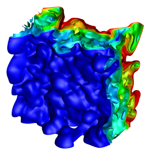
Figure 1. (a) Comparison of MW  $\delta _{MZ}$ between current CLES (solid line), experiment by Vetter & Sturtevant (Reference Vetter and Sturtevant1995) (squares), ILES by Schilling & Latini (Reference Schilling and Latini2010) (dash line) and RANS model by Xiao et al. (Reference Xiao, Zhang and Tian2020a) (dash-dot line). (b) Three-dimensional isosurface of
  $\tilde {\psi }$ at
  $t=0.01\ \mathrm {s}$.
4.2. Mixing zone structure
As mention before, compared with the model, the most important advantage of the LES is that it can capture the three-dimensional large-scale structure. As for mixing, the evolution of structure is very important in understanding some critical mixing mechanisms. These mechanisms include the early growth of structure (i.e. bubbles and spikes at the two edges), and the later merging of the neighbouring structure during the stage of self-similar turbulent mixing. In figure 1(b), we plot the three-dimensional iso-surface of  $\tilde {\psi }$ at
  $t=0.010\ \mathrm {s}$. From these figures, we can see that the large-scale structures are well resolved in the current CLES methods.
4.3. Mixed mass
Another important quantity to characterize the evolution of mixing layers is the mixed mass. The normalized mixed mass proposed by Zhou et al. (Reference Zhou, Cabot and Thornber2016) measures the efficiency of the mixed mass. The definitions of the mixed mass  $M$ and the normalized mixed mass
  $\varPsi$ are given by
 \begin{equation} M \equiv \int 4 \bar{\rho} \tilde{\psi}_1 \tilde{\psi}_2 \,\textrm{d}V,\quad \varPsi \equiv \frac{\displaystyle\int \bar{\rho} \tilde{\psi}_1 \tilde{\psi}_2 \,\textrm{d}V}{\displaystyle\int \langle\bar{\rho}\rangle \langle\tilde{\psi}_1\rangle \langle\tilde{\psi}_2\rangle \,\textrm{d}V}. \end{equation}
Compared with other traditional mixedness parameters, the normalized mixed mass is able to provide more consistent result for both RT instability and RM instability flows. We plot the evolution of mixed mass and normalized mixed mass calculated from CLES in figures 2(a) and 2(b), respectively. The evolution of the mixed mass  $M$ is similar to that of the MW in figure 1(a). This similar behaviour also exists in RT instability (Zhou et al. Reference Zhou, Cabot and Thornber2016; Zhang et al. Reference Zhang, Ni, Ruan and Xie2020b). The normalized mixed mass converges to a constant when the flow is fully developed.

Figure 2. The evolution of (a) mixed mass and (b) normalized mixed mass calculated from CLES.
5. Conclusion and discussion
Accurately predicting the evolution of spatial structure and MW of reshocked RM mixing is of fundamental importance. Currently, the most viable method is LES. However, satisfactory LES prediction has not been previously achieved. To achieve this prediction, in this paper, we successfully extend the CLES from single-medium turbulence to multi-media turbulence. Specifically, based on the Reynolds decomposition, the unclosed SGS terms of LES are decomposed into the averaging part and fluctuating part. The former dominates the evolution of the mean fields, while the latter affects the evolution of structure. Therefore, to accurately predict the mean fields, the averaging part is modelled by requiring that the Reynolds averaged LES equation takes the same form as that of the RANS equation, which is the main idea of CLES. The fluctuating part is modelled with the traditional SGS model. Consequently, the mean field calculated by the CLES model predominantly depends on the RANS model, while the spatial structure and the (normalized) mixed mass predominantly depend on the traditional SGS model. To guarantee an accurate prediction, the most accurate  $K$-
$K$- $L$ model given by Xiao et al. (Reference Xiao, Zhang and Tian2020a) is used in the RANS model, while the classical Smagorinsky model is used for the SGS model. In a word, the CLES model provides a way to combine the RANS model and the traditional SGS model.
With a very coarse grid, the current CLES successfully captures the MW growth of reshocked RM mixing, as well as the evolution of three-dimensional large-scale spatial structure and the (normalized) mixed mass. To the best of our knowledge, this is the first time that LES is able to give such a comparable result with Vetter & Sturtevant's benchmark experimental results for reshocked RM mixing. The CLES provided a new way to simulate multi-media turbulence. In the future, we plan to extend this method to more challenging problems that have not been well predicted with traditional SGS models, e.g. mixing problems with converging and complex geometries.
Acknowledgements
The authors want to thank Dr H.-F. Li, Mr Y.-C. Ruan and Ms H. Li for their helpful insights, and anonymous referees for their professional comments and helpful English editing assistance, which have greatly improved the quality of this paper.
Funding
This work was supported by the National Natural Science Foundation of China (NSFC) (Y.-P.S., grant number 91752202), (Y.-S.Z., grant number 11972093), (M.-J.X., grant number 12002059).
Declaration of interests
The authors report no conflict of interest.


