2.1. Inviscid case

Any quantity, $\psi$ say, associated with internal gravity waves in an inviscid uniformly stratified Boussinesq fluid satisfies an equation of the form

(2.1)\begin{equation} \left(\frac{\partial^{2}}{\partial t^{2}}\boldsymbol{\nabla}^{2}+N^{2}\boldsymbol{\nabla}_{\mathrm{h}}^{2}\right) \psi =q, \end{equation}

where $N$ is the buoyancy frequency, $z$ the vertical coordinate, $\boldsymbol{\nabla} = (\partial /\partial x,\partial /\partial y,\partial /\partial z)$ the del operator, $\boldsymbol{\nabla} _{\mathrm {h}} = (\partial /\partial x,\partial /\partial y,0)$ its original projection and $q$ a source term; see, for example, Lighthill (Reference Lighthill1978, § 4.1) or Voisin (Reference Voisin1991). Assuming the source to be two-dimensional and monochromatic, $q = f(x,z)\exp (-\mathrm {i}\omega _0t)$ with $\omega _0 < N$, and introducing Fourier transforms according to

(2.2a)\begin{gather} f(k,m) = \iint f(x,z)\exp[-\mathrm{i}(kx+mz)]\,\mathrm{d}x\,\mathrm{d}z, \end{gather}

(2.2b)\begin{gather} f(x,z) = \frac{1}{(2\pi)^{2}}\iint f(k,m)\exp[\mathrm{i}(kx+mz)]\,\mathrm{d}k\,\mathrm{d}m, \end{gather}

the solution of (2.1) follows as

(2.3)\begin{equation} \psi = \frac{\exp(-\mathrm{i}\omega_0t)}{4\pi^{2}}\iint \frac{f(k,m)\exp[\mathrm{i}(kx+mz)]}{\omega_0^{2}\kappa^{2}-N^{2}k^{2}}\,\mathrm{d}k\,\mathrm{d}m, \end{equation}

with $\textbf {{x}} = (x,z)$ the position, ${\boldsymbol {k}} = (k,m)$ the wavenumber vector and $r = (x^{2}+z^{2})^{1/2}$ and $\kappa = (k^{2}+m^{2})^{1/2}$ their moduli.

Lighthill devised a method for the asymptotic evaluation of such Fourier integral in the far field, as $r \to \infty$, first for a rapidly decreasing source (Reference Lighthill1960) then for a source of compact support (Reference Lighthill1978, § 4.9), with identical results. We adopt the former, more general presentation; namely, the source function $f(x,z)$ is assumed to decrease asymptotically faster than any inverse power of $x$ or $z$, so that its spectrum $f(k,m)$ is a regular function of the real variables $k$ and $m$.

The asymptotic behaviour of the integral is expressed in terms of the singularities of the integrand (Lighthill Reference Lighthill1958, chapter 4). Given the regularity of $f(k,m)$, these are the solutions of the dispersion relation

(2.4)\begin{equation} B(\omega_0,{\boldsymbol {k}}) = \omega_0^{2}\kappa^{2}-N^{2}k^{2} = 0. \end{equation}

In the wavenumber plane this defines a wavenumber curve, represented in figure 1, in the shape of a St Andrew's cross with arms inclined at the angle $\theta _0 = \arccos (\omega _0/N)$ to the horizontal. Writing

(2.5a,b)\begin{equation} \omega_0 = N\frac{|k|}{\kappa},\quad {\boldsymbol {c}}_{\mathrm{g}} = \left(\frac{\partial\omega_0}{\partial k},\frac{\partial\omega_0}{\partial m}\right) = N\frac{m}{\kappa^{3}}(m,-k)\ \textrm{sign}\ k, \end{equation}

the group velocity ${\boldsymbol {c}}_{\mathrm {g}}$, at which the wave energy propagates, is seen to be perpendicular to ${\boldsymbol {k}}$. Accordingly, each arm of the cross radiates waves perpendicular to itself, forming another St Andrew's cross in the physical plane, represented in figure 2, with arms inclined at the angle $\theta _0$ to the vertical.

Figure 1. Wavenumber curve for two-dimensional internal waves.

Figure 2. Wave beams for two-dimensional internal waves.

We introduce characteristic coordinates $(x_\pm,z_\pm )$ such that

(2.6a,b)\begin{equation} x_\pm = x\cos\theta_0\mp z\sin\theta_0, \quad z_\pm = \pm x\sin\theta_0+z\cos\theta_0, \end{equation}

and associated wavenumbers $(k_\pm,m_\pm )$ such that

(2.7a,b)\begin{equation} k_\pm = k\cos\theta_0\mp m\sin\theta_0, \quad m_\pm = \pm k\sin\theta_0+m\cos\theta_0, \end{equation}

as shown in figures 1 and 2. The dispersion relation simplifies to

(2.8)\begin{equation} B(\omega_0,{\boldsymbol {k}}) = N^{2}m_+m_- = 0, \end{equation}

and the equation of the wavenumber curve to

(2.9)\begin{equation} m_\pm = 0. \end{equation}

The group velocity becomes

(2.10)\begin{equation} {\boldsymbol {c}}_{\mathrm{g}} = \pm\frac{N\sin\theta_0}{k_\pm}{\boldsymbol {e}}_{z_{\,\pm}}, \end{equation}

with

(2.11)\begin{equation} {\boldsymbol {e}}_{z_\pm} = \pm{\boldsymbol {e}}_x\sin\theta_0+{\boldsymbol {e}}_z\cos\theta_0 \end{equation}

a unit vector along the $z_\pm$-axis. The two halves $k_\pm < 0$ and $k_\pm > 0$ of each arm $m_\pm = 0$ of the cross are seen to radiate waves in opposite directions, shown in figure 1.

The contribution of each arm to integral (2.3) is evaluated in coordinates $(k_\pm,m_\pm )$, writing

(2.12)\begin{equation} \psi = \frac{\exp(-\mathrm{i}\omega_0t)}{4\pi^{2}} \int_{-\infty}^{\infty}\mathrm{d}k_\pm \exp(\mathrm{i}k_\pm x_\pm) \int_{-\infty}^{\infty} \frac{f_\pm(k_\pm,m_\pm)}{B(\omega_0,{\boldsymbol {k}})} \exp(\mathrm{i}m_\pm z_\pm)\,\mathrm{d}m_\pm, \end{equation}

where $f_\pm (k_\pm,m_\pm ) = f(k,m)$, then allowing $m_\pm$ to become complex and applying the residue theorem to the inner integral. An additional condition is required to displace the real pole (2.9) slightly off the path of integration. For this, Lighthill (Reference Lighthill1960, Reference Lighthill1978, § 4.9) introduced an innovative formulation of the radiation condition, giving the frequency an infinitesimal positive imaginary part $\epsilon \ll N$. The dispersion relation becomes

(2.13)\begin{equation} B(\omega_0+\mathrm{i}\epsilon,{\boldsymbol {k}}) \sim N^{2} \left[m_\pm m_\mp+2\mathrm{i}\frac{\epsilon}{N}(k_\pm^{2}+m_\pm^{2})\cos\theta_0\right] = 0, \end{equation}

where

(2.14)\begin{equation} m_\mp = \mp k_\pm\sin(2\theta_0)+m_\pm\cos(2\theta_0), \end{equation}

providing a second-order equation for $m_\pm$ as a function of $k_\pm$. To leading order in $\epsilon /N$, the pole (2.9) is displaced to

(2.15)\begin{equation} m_\pm \sim \pm\mathrm{i}\frac{\epsilon}{N\sin\theta_0}k_\pm. \end{equation}

The path of integration is raised or lowered a distance $\mu$ depending on whether $z_\pm > 0$ or $z_\pm < 0$, respectively, so as to make the integral $O[\exp (-\mu |z_\pm |)]$. With an error of this order, the integral evaluates to $2\mathrm {i}\pi\ \textrm{sign}\ z_\pm$ times the sum of the residues of the integrand at any poles passed over in deforming the path. Given the regularity of $f_\pm (k_\pm,m_\pm )$ for real $m_\pm$, and provided that $\epsilon$ is small enough, $\mu$ may be chosen such that no complex singularity of $f_\pm (k_\pm,m_\pm )$ is passed over, if any, and the only pole to consider is (2.15).

This procedure picks the pole with an imaginary part of the same sign as $z_\pm$, namely

(2.16)\begin{equation} m_\pm \sim \mathrm{i}\frac{\epsilon}{N\sin\theta_0}|k_\pm|\ \textrm{sign}\ z_\pm, \end{equation}

subject to the condition

(2.17)\begin{equation} \hbox{sign}\ k_\pm = \pm\ \textrm{sign}\ z_\pm, \end{equation}

thereby allowing only one half of the arm of the cross to contribute to the radiation. Physically, this amounts to imposing ${\boldsymbol {c}}_{\mathrm {g}}\boldsymbol \cdot {\boldsymbol {x}} > 0$, with ${\boldsymbol {x}} = (x,z)$ the position, namely to selecting the part of the wavenumber curve such that the component of the group velocity along the direction of observation points outwards not inwards, consistent with figure 1. The introduction of $\epsilon$ has fulfilled its use, and we may now let $\epsilon \to 0$ to get

(2.18)\begin{equation} m_\pm = 0 \quad \text{with}\ \textrm{sign}\ k_\pm = \pm\ \textrm{sign}\ z_\pm. \end{equation}

An asymptotic expansion of the waves follows,

(2.19)\begin{equation} \psi \sim -\mathrm{i}\frac{\exp(-\mathrm{i}\omega_0t)} {4\pi N^{2}\sin\theta_0\cos\theta_0}\int_0^{\pm\infty\ \textrm{sign}\ z_\pm} f_\pm(k_\pm,m_\pm = 0) \exp(\mathrm{i}k_\pm x_\pm)\frac{\mathrm{d}k_\pm}{k_\pm}, \end{equation}

valid in the far field as $|z_\pm | \to \infty$. It was first obtained by Lighthill (Reference Lighthill1978, § 4.10).

We are looking for an exact expression of the waves in the near field, at finite $|z_\pm |$. For this, more restrictive assumptions must be made about the source, which is assumed to be of compact support of radius $a$, in the sense that $f(x,z) = 0$ for $r > a$. The spectrum $f_\pm (k_\pm,m_\pm )$, being an integral over a finite domain, is an analytic function of the complex wavenumbers $k_\pm$ and $m_\pm$; for each of them its modulus decreases asymptotically along the real axis, is small for $|\operatorname {Re} k_\pm | \gtrsim 1/a$ or $|\operatorname {Re} m_\pm | \gtrsim 1/a$, and grows exponentially along the imaginary axis. Specifically, we have

(2.20)\begin{equation} |\,f_\pm(k_\pm,m_\pm)| < \exp[a(|\operatorname{Im} k_\pm|+|\operatorname{Im} m_\pm|)] \iint_{r < a}|\,f(x,z)|\,\mathrm{d}x\,\mathrm{d}z. \end{equation}

This bound allows the path of integration of the inner integral in (2.12) to be closed by a semi-circle at infinity in the half-plane where the imaginary part of $m_\pm$ is of the same sign as $z_\pm$: by a straightforward extension of Jordan's lemma, the contribution of the semi-circle vanishes provided that $|z_\pm | > a$, and the integral evaluates to $2\mathrm {i}\pi \ \textrm {sign} \ z_\pm$ times the sum of the residues of the integrand at any poles with an imaginary part of the same sign as $z_\pm$.

Given the analyticity of $f_\pm (k_\pm,m_\pm )$, the only pole to consider is, again, (2.16). The waves follow immediately, when both $|z_+| > a$ and $|z_-| > a$, as

(2.21)\begin{equation} \psi = -\mathrm{i}\frac{\exp(-\mathrm{i}\omega_0t)} {4\pi N^{2}\sin\theta_0\cos\theta_0} \sum_\pm \int_0^{\pm\infty\ \textrm{sign}\ z_\pm} f_\pm(k_\pm,m_\pm = 0) \exp(\mathrm{i}k_\pm x_\pm)\frac{\mathrm{d}k_\pm}{k_\pm}, \end{equation}

or, equivalently,

(2.22)\begin{align} \psi &= -\mathrm{i}\frac{\exp(-\mathrm{i}\omega_0t)} {4\pi N^{2}\sin\theta_0\cos\theta_0}\sum_\pm \int_0^{\infty} f_\pm(k_\pm = \pm\kappa\ \textrm{sign}\ z_\pm,m_\pm = 0) \nonumber\\ &\quad \times \exp(\pm\mathrm{i}\kappa x_\pm\ \hbox{sign}\ z_\pm)\frac{\mathrm{d}\kappa}{\kappa}. \end{align}

As a result, if four wave beams are defined as the contributions of the four half-arms of the wavenumber curve, then at any given location two beams are received, one for the half $\textrm {sign} \ k_+ = \textrm {sign}\ z_+$ of the arm $m_+ = 0$, and the other for the half $\textrm {sign} \ k_- = -\textrm {sign} \ z_-$ of the arm $m_- = 0$. In the far field, as $|z_\pm | \to \infty$ with $x_\pm$ fixed, the contribution of one arm $m_\pm = 0$ becomes dominant compared with that for the other arm $m_\mp = 0$; then (2.19) is recovered and each beam turns into a half-arm of the St Andrew's cross shown in figure2 and observed experimentally by Görtler (Reference Görtler1943), Mowbray & Rarity (Reference Mowbray and Rarity1967), Sutherland etal. (Reference Sutherland, Dalziel, Hughes and Linden1999) and Zhang etal. (Reference Zhang, King and Swinney2007), among others.

Conversely, the line $z_+ = 0$ is seen to separate the two beams $k_+ < 0$ and $k_+ > 0$ originating from the arm $m_+ = 0$ of the wavenumber curve, and the line $z_- = 0$ the two beams $k_- < 0$ and $k_- > 0$ originating from the arm $m_- = 0$. For each beam, (2.22) is ascertained to be valid from the distance $|z_\pm | = a$ where the beam leaves the source behind, up to infinity. Being based on an upper bound (2.20), it can be valid closer to the source, depending on the exact form of $f_\pm (k_\pm,m_\pm )$; this, however, can only be assessed on a case-by-case basis, as will be seen later in § 8.1.

2.2. Viscous case

Viscosity acts as another equivalent way of setting which part of the wavenumber curve is received at which location. The wave equation becomes

(2.23)\begin{equation} \left[\left(\frac{\partial}{\partial t}-\nu\boldsymbol{\nabla}^{2}\right) \frac{\partial}{\partial t}\boldsymbol{\nabla}^{2}+N^{2}\boldsymbol{\nabla}_{\mathrm{h}}^{2}\right]\psi = q, \end{equation}

with $\nu$ the kinematic viscosity; see, for example, Voisin (Reference Voisin2003). The response to two-dimensional monochromatic forcing becomes

(2.24)\begin{equation} \psi = \frac{\exp(-\mathrm{i}\omega_0t)}{4\pi^{2}}\iint \frac{f(k,m)\exp[\mathrm{i}(kx+mz)]}{\omega_0^{2}\kappa^{2}-N^{2}k^{2}+\mathrm{i}\omega_0\nu\kappa^{4}}\mathrm{d}k\,\mathrm{d}m. \end{equation}

Lighthill (Reference Lighthill1978, § 4.10) did not evaluate this integral directly. Instead, he calculated the shear-induced rate of energy dissipation along the rays of a plane internal wave (Lighthill Reference Lighthill1978, § 4.7), then deduced from it an exponential attenuation factor to be added inside the inviscid expansion (2.19).

We proceed from (2.24), on the assumption $\nu \kappa ^{2}/N \ll 1$ of small viscous effects. The addition of viscosity transforms the dispersion relation (2.8) into

(2.25)\begin{equation} B(\omega_0,{\boldsymbol {k}}) = N^{2} \left[m_\pm m_\mp+\mathrm{i}\frac{\nu}{N}(k_\pm^{2}+m_\pm^{2})^{2}\cos\theta_0\right]= 0, \end{equation}

with $m_\mp$ given by (2.14), thus providing a fourth-order equation for $m_\pm$. To leading order in $\nu k_\pm ^{2}/N$, the pole (2.9) is displaced to

(2.26)\begin{equation} m_\pm \sim \pm\mathrm{i}\beta k_\pm^{3}, \end{equation}

where

(2.27)\begin{equation} \beta = \frac{\nu}{2N\sin\theta_0}. \end{equation}

The above deformations of contour pick

(2.28)\begin{equation} m_\pm \sim \mathrm{i}\beta|k_\pm^{3}|\ \textrm{sign}\ z_\pm \quad \text{with}\ \textrm{sign}\ k_\pm = \pm\ \textrm{sign}\ z_\pm, \end{equation}

yielding for a rapidly decreasing source the far-field expansion, as $|z_\pm | \to \infty$,

(2.29)\begin{align} \psi &\sim -\mathrm{i}\frac{\exp(-\mathrm{i}\omega_0t)} {4\pi N^{2}\sin\theta_0\cos\theta_0}\int_0^{\pm\infty\ \textrm{sign}\ z_\pm} f_\pm(k_\pm,m_\pm = \mathrm{i}\beta|k_\pm^{3}|\ \textrm{sign}\ z_\pm) \nonumber\\ &\quad\times \exp(-\beta|k_\pm^{3}z_\pm|)\exp(\mathrm{i}k_\pm x_\pm)\frac{\mathrm{d}k_\pm}{k_\pm}, \end{align}

and for a source of compact support the exact expression, valid when both $|z_+| > a$ and $|z_-| > a$,

(2.30)\begin{align} \psi &= -\mathrm{i}\frac{\exp(-\mathrm{i}\omega_0t)}{4\pi N^{2}\sin\theta_0\cos\theta_0} \sum_\pm \int_0^{\pm\infty\ \textrm{sign}\ z_\pm} f_\pm(k_\pm,m_\pm = \mathrm{i}\beta|k_\pm^{3}|\ \textrm{sign}\ z_\pm) \nonumber\\ &\quad \times \exp(-\beta|k_\pm^{3}z_\pm|) \exp(\mathrm{i}k_\pm x_\pm)\frac{\mathrm{d}k_\pm}{k_\pm}, \end{align}

or, equivalently,

(2.31)\begin{align} \psi &= -\mathrm{i}\frac{\exp(-\mathrm{i}\omega_0t)}{4\pi N^{2}\sin\theta_0\cos\theta_0} \sum_\pm \int_0^{\infty} f_\pm(k_\pm = \pm\kappa\ \textrm{sign}\ z_\pm,m_\pm = \mathrm{i}\beta\kappa^{3}\ \textrm{sign}\ z_\pm) \nonumber\\ &\quad \times \exp(-\beta\kappa^{3}|z_\pm|) \exp(\pm\mathrm{i}\kappa x_\pm\ \textrm{sign}\ z_\pm) \frac{\mathrm{d}\kappa}{\kappa}. \end{align}

A new difference arises with Lighthill's (Reference Lighthill1978, § 4.10) far-field analysis, in addition to the superposition of two wave beams at any given location; namely, the occurrence of the viscous correction (2.28) to the wavenumber not only for the propagation of the waves, as an attenuation factor, but also for their generation, inside the source spectrum. The relevance of this correction will be discussed later in § 8.1.

2.3. Validity

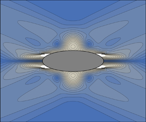
The preceding analysis is essentially a reformulation of the far-field expansion of Lighthill (Reference Lighthill1978, § 4.10) for rapidly decreasing sources, and its extension to the near field for the smaller class of sources of compact support. The solutions of Hurley (Reference Hurley1997) and Hurley & Keady (Reference Hurley and Keady1997) for the oscillations of an elliptic cylinder are of the type anticipated by Lighthill. When the cylinder is circular, the experiments of Sutherland etal. (Reference Sutherland, Dalziel, Hughes and Linden1999) and Zhang etal. (Reference Zhang, King and Swinney2007) have confirmed their quantitative validity not only in the far field but also in the near field. When the cylinder is elliptic, the comparison with the experiments of Sutherland & Linden (Reference Sutherland and Linden2002) has been less conclusive. The wave structure for the circular cylinder is illustrated in figure 3(a), where both beam separation and viscous attenuation are set by the along-beam coordinates $z_\pm$.

Figure 3. Structure of the beams propagating upward to the right and downward to the left for (a) a circular cylinder, (b) a horizontal segment and (c) an elliptic cylinder. The beams are delimited by the critical rays grazing the oscillating body at critical points on either side. The grey areas represent the zones where the validity of the theory is not ascertained.

The same is not true of all sources though: when the source is infinitely thin, beam separation and viscous attenuation are set by the normal coordinate to the source, $z$ for the horizontal segment in figure 3(b). Adapting the results of Tilgner (Reference Tilgner2000), Bardakov etal. (Reference Bardakov, Vasil'ev and Chashechkin2007), Davis & Llewellyn Smith (Reference Davis and Llewellyn Smith2010) and Le Dizès (Reference Le Dizès2015) for the oscillations of a horizontal circular disc to the line source $q = g(x)\delta (z)\exp (-\mathrm {i}\omega _0 t)$, with $\delta$ the Dirac delta function, we obtain

(2.32)\begin{align} \psi &= -\mathrm{i}\frac{\exp(-\mathrm{i}\omega_0t)} {4\pi N^{2}\sin\theta_0\cos\theta_0}\sum_\pm\int_0^{\pm\infty\ \textrm{sign}\ z} g(k = k_\pm\cos\theta_0) \nonumber\\ &\quad \times \exp(-\beta|k_\pm^{3}z|/\cos\theta_0) \exp(\mathrm{i}k_\pm x_\pm) \frac{\mathrm{d}k_\pm}{k_\pm}, \end{align}

or, equivalently,

(2.33)\begin{align} \psi &= -\mathrm{i}\frac{\exp(-\mathrm{i}\omega_0t)} {4\pi N^{2}\sin\theta_0\cos\theta_0}\sum_\pm\int_0^{\infty} g(k = \pm\kappa\cos\theta_0\ \textrm{sign}\ z) \nonumber\\ &\quad \times\exp(-\beta\kappa^{3}|z|/\cos\theta_0) \exp(\pm\mathrm{i}\kappa x_\pm\ \textrm{sign}\ z)\frac{\mathrm{d}\kappa}{\kappa}. \end{align}

At first glance the two wave structures, shown in figure 3(a,b), appear incompatible with each other. In particular, the spectrum $f(k,m) = g(k)$ of the line source leaves the normal wavenumber $m$ arbitrary, thereby allowing $|k_\pm |$ to become infinitely large and preventing the pole displacements (2.15) and (2.26) from remaining small, however small $\epsilon /N$ and $\beta \kappa ^{2}$ can be.

In order to elucidate the effect of the geometry of the source on its wave radiation, we consider a source of elliptic shape in the following. The anticipated wave structure is illustrated in figure 3(c) for an elliptic cylinder, with both beam separation and viscous attenuation set by the normal distance to the line joining the two critical points where critical wave rays are tangential to the cylinder on either side. After a brief derivation of the wave equation in the following section, we will move on to the determination of the fluid velocity.

4.1. Inviscid case

To proceed further, we start with the inviscid case and introduce the lengths

(4.5)\begin{equation} c_\pm = [a^{2}\cos^{2}(\theta_0\pm\varphi_0)+b^{2}\sin^{2}(\theta_0\pm\varphi_0)]^{1/2}, \end{equation}

the angles $\Theta _\pm$ such that

(4.6a,b)\begin{equation} \cos\Theta_\pm = \frac{a}{c_\pm}\cos(\theta_0\pm\varphi_0), \quad \sin\Theta_\pm = \frac{b}{c_\pm}\sin(\theta_0\pm\varphi_0), \end{equation}

and the rescaled characteristic coordinates

(4.7a,b)\begin{equation} X_\pm = X_0\cos\Theta_\pm\mp Z_0\sin\Theta_\pm, \quad Z_\pm = \pm X_0\sin\Theta_\pm+Z_0\cos\Theta_\pm, \end{equation}

and similarly $(K_\pm,M_\pm )$ in the wavenumber plane. These quantities are best interpreted by considering an elliptic cylinder of semi-axes $a$ and $b$, illustrated in figure 4. Then, as pointed out by Hurley (Reference Hurley1997), $c_+$ and $c_-$ are the half-widths of the wave beams delimited by the critical rays tangential to the cylinder on either side.

Figure 4. Geometry of the beams propagating (a) upward to the right and downward to the left, and (b) upward to the left and downward to the right, for the oscillations of an elliptic cylinder.

The dispersion relation (2.8) becomes

(4.8)\begin{equation} B(\omega_0,{\boldsymbol {k}}) = N^{2}\frac{c_+c_-}{a^{2}b^{2}}M_+M_- = 0, \end{equation}

implying that the wavenumber curve is still a St Andrew's cross but its arms now make different angles to the horizontal, $\Theta _+$ for the arm $M_+ = 0$ and $\Theta _-$ for the arm $M_- = 0$. Proceeding as in § 2, we evaluate the contribution of each arm in coordinates $(K_\pm,M_\pm )$, allowing $M_\pm$ to become complex and applying the residue theorem. The radiation condition transforms the dispersion relation into

(4.9)\begin{equation} B(\omega_0+\mathrm{i}\epsilon,{\boldsymbol {k}}) \sim N^{2}\left(\frac{c_+c_-}{a^{2}b^{2}}M_\pm M_\mp+2\mathrm{i}\frac{\epsilon}{N}\kappa^{2}\cos\theta_0\right) = 0, \end{equation}

where

(4.10)\begin{equation} M_\mp = \mp K_\pm\sin(\Theta_++\Theta_-)+M_\pm\cos(\Theta_++\Theta_-), \end{equation}

and

(4.11)\begin{equation} \kappa^{2} = \frac{1}{c_\pm^{2}}K_\pm^{2} +\left(\frac{\sin^{2}\Theta_\pm}{a^{2}}+\frac{\cos^{2}\Theta_\pm}{b^{2}}\right)M_\pm^{2} \pm 2\left(\frac{1}{a^{2}}-\frac{1}{b^{2}}\right)K_\pm M_\pm \sin\Theta_\pm\cos\Theta_\pm, \end{equation}

displacing the pole $M_\pm = 0$ to

(4.12)\begin{equation} M_\pm \sim \pm\mathrm{i}\frac{ab}{c_\pm^{2}}\frac{\epsilon}{N\sin\theta_0}K_\pm. \end{equation}

Now, the spectrum $F_\pm (K_\pm,M_\pm ) = F_0(K_0,M_0) = f_0(k_0,m_0)$ is an analytic function of the complex wavenumbers $K_\pm$ and $M_\pm$, for each decreasing asymptotically along the real axis, small for $|\operatorname {Re} K_\pm | \gtrsim 1$ or $|\operatorname {Re} M_\pm | \gtrsim 1$, and growing exponentially along the imaginary axis, with

(4.13)\begin{equation} |F_\pm(K_\pm,M_\pm)| < \exp(|\operatorname{Im} K_\pm|+|\operatorname{Im} M_\pm|) \iint_{|{\boldsymbol {X}}_0| < 1}|F_0(X_0,Z_0)|\,\mathrm{d}X_0\,\mathrm{d}Z_0 . \end{equation}

Accordingly, the real path of integration for the variable $M_\pm$ may be closed by a semi-circle at infinity in the half-plane where the imaginary part of $M_\pm$ is of the same sign as $Z_\pm$, in such a way that the contribution of the semi-circle vanishes for $|Z_\pm | > 1$. The integral follows as $2\mathrm {i}\pi \ \textrm {sign} \ Z_\pm$ times the sum of the residues of the integrand at any poles with an imaginary part of the same sign as $Z_\pm$. This procedure picks the pole

(4.14)\begin{equation} M_\pm \sim \mathrm{i}\frac{ab}{c_\pm^{2}}\frac{\epsilon}{N\sin\theta_0}|K_\pm|\ \textrm{sign}\ Z_\pm \quad \text{with}\ \textrm{sign}\ K_\pm = \pm\ \textrm{sign}\ Z_\pm. \end{equation}

With $\epsilon /N \ll 1$ and $|K_\pm | = O(1)$, the displacement is small and the limit $\epsilon \to 0$ may be applied, so that

(4.15)\begin{equation} M_\pm = 0 \quad \text{with} \ \textrm{sign}\ K_\pm = \pm\ \textrm{sign}\ Z_\pm. \end{equation}

The evaluation of the waves is then immediate when $|Z_+| > 1$ and $|Z_-| > 1$, yielding

(4.16)\begin{equation} {\boldsymbol {u}} = \frac{\exp(-\mathrm{i}\omega_0t)}{4\pi} \sum_\pm (\pm) \frac{{\boldsymbol {e}}_{z_\pm}}{c_\pm}\int_0^{\pm\infty\ \textrm{sign}\ Z_\pm} F_\pm(K_\pm,M_\pm = 0) \exp(\mathrm{i}K_\pm X_\pm) \,\mathrm{d}K_\pm. \end{equation}

To go back to unscaled coordinates, we introduce the new lengths

(4.17)\begin{equation} d_\pm = (a^{2}\cos^{2}\Theta_\pm+b^{2}\sin^{2}\Theta_\pm)^{1/2} = \frac{[a^{4}\cos^{2}(\theta_0\pm\varphi_0)+b^{4}\sin^{2}(\theta_0\pm\varphi_0)]^{1/2}}{c_\pm}, \end{equation}

the new angles $\chi _\pm$ such that

(4.18a)\begin{gather} \cos\chi_\pm = \frac{a}{d_\pm}\cos\Theta_\pm = \frac{a^{2}}{c_\pm d_\pm}\cos(\theta_0\pm\varphi_0), \end{gather}

(4.18b)\begin{gather}\sin\chi_\pm = \frac{b}{d_\pm}\sin\Theta_\pm = \frac{b^{2}}{c_\pm d_\pm}\sin(\theta_0\pm\varphi_0), \end{gather}

and the new coordinates

(4.19a,b)\begin{equation} \xi_\pm = x_0\cos\chi_\pm\mp z_0\sin\chi_\pm, \quad \zeta_\pm = \pm x_0\sin\chi_\pm+z_0\cos\chi_\pm, \end{equation}

and similarly $(\kappa _\pm,\mu _\pm )$ in the wavenumber plane. For the elliptic cylinder, $d_+$ and $d_-$ are the half-lengths of the critical segments joining the critical points where the critical rays are tangential to the cylinder on either side, and $\chi _+$ and $\chi _-$ are the angles of these segments to the positive $x_0$-axis, counted clockwise for $\chi _+$ and counterclockwise for $\chi _-$, as shown in figure 4.

We have

(4.20a–c)\begin{equation} X_\pm = \frac{x_\pm}{c_\pm}, \quad Z_\pm = \zeta_\pm\frac{d_\pm}{ab},\quad K_\pm = \kappa_\pm d_\pm,\quad M_\pm = m_\pm\frac{ab}{c_\pm}. \end{equation}

Furthermore, on the wavenumber curve $M_\pm = 0$, we also have $m_\pm = 0$ and $K_\pm = k_\pm c_\pm$. It then follows that, when both $|\zeta _+| > ab/d_+$ and $|\zeta _-| > ab/d_-$,

(4.21)\begin{align} {\boldsymbol {u}} &= \frac{\exp(-\mathrm{i}\omega_0t)}{4\pi} \sum_\pm {\boldsymbol {e}}_{z_\pm}\ \textrm{sign}\ \zeta_\pm \int_0^{\infty} f_\pm(k_\pm = \pm\kappa\ \textrm{sign}\ \zeta_\pm,m_\pm = 0) \nonumber\\ &\quad \times \exp(\pm\mathrm{i}\kappa x_\pm\ \textrm{sign}\ \zeta_\pm)\,\mathrm{d}\kappa, \end{align}

where $\kappa = |k_\pm | = |K_\pm |/c_\pm$. Consistent with figure 3(c), beam separation is set by the coordinates $\zeta _\pm$ normal to the critical lines.

4.2. Viscous case

The presence of viscosity transforms the dispersion relation (4.8) into

(4.22)\begin{equation} B(\omega_0,{\boldsymbol {k}}) = N^{2} \left(\frac{c_+c_-}{a^{2}b^{2}}M_\pm M_\mp+\mathrm{i}\frac{\nu}{N}\kappa^{4}\cos\theta_0 \right) = 0. \end{equation}

There are now four poles, whose contributions are evaluated in the small-viscosity limit $Nc_+c_-/\nu \gg 1$, corresponding to a large Stokes number.

Two poles are associated with waves,

(4.23)\begin{equation} M_\pm \sim \pm\mathrm{i}\beta\frac{ab}{c_\pm^{4}}K_\pm^{3}, \end{equation}

where $\beta$ has been defined in (2.27). Closing the path of integration as above picks the pole

(4.24)\begin{equation} M_\pm \sim \mathrm{i}\beta\frac{ab}{c_\pm^{4}}|K_\pm|^{3}\ \hbox{sign}\ Z_\pm \quad \text{with} \ \textrm{sign}\ K_\pm = \pm\ \textrm{sign}\ Z_\pm. \end{equation}

The assumptions $\beta /c_\pm ^{2} \ll 1$ and $|K_\pm | = O(1)$ ensure its smallness. Setting it to zero in the slowly varying rational fraction in the integrand of (4.3) when evaluating the residue, but keeping it non-zero in the spectrum and in the rapidly varying complex exponential, the velocity follows for $|Z_+| > 1$ and $|Z_-| > 1$ as

(4.25)\begin{align} {\boldsymbol {u}} &= \frac{\exp(-\mathrm{i}\omega_0t)}{4\pi} \sum_\pm(\pm) \frac{{\boldsymbol {e}}_{z_\pm}}{c_\pm} \int_0^{\pm\infty\ \textrm{sign}\ Z_\pm} F_\pm \left(K_\pm, M_\pm = \mathrm{i}\beta\frac{ab}{c_\pm^{4}}|K_\pm|^{3}\ \textrm{sign}\ Z_\pm\right) \nonumber\\ &\quad \times \exp\left(-\beta\frac{ab}{c_\pm^{4}}|K_\pm^{3}Z_\pm|\right) \exp(\mathrm{i}K_\pm X_\pm) \,\mathrm{d}K_\pm, \end{align}

that is, in unscaled coordinates, for $|\zeta _+| > ab/d_+$ and $|\zeta _-| > ab/d_-$,

(4.26)\begin{align} {\boldsymbol {u}} &= \frac{\exp(-\mathrm{i}\omega_0t)}{4\pi} \sum_\pm {\boldsymbol {e}}_{z_\pm}\ \textrm{sign}\ \zeta_\pm \int_0^{\infty} F_\pm \left(K_\pm = \pm\kappa c_\pm\ \textrm{sign}\ \zeta_\pm, M_\pm = \mathrm{i}\beta\kappa^{3}\frac{ab}{c_\pm}\ \textrm{sign}\ \zeta_\pm\right) \nonumber\\ &\quad \times \exp\left(-\beta\kappa^{3}\frac{d_\pm}{c_\pm}|\zeta_\pm|\right) \exp(\pm\mathrm{i}\kappa x_\pm\ \textrm{sign}\ \zeta_\pm)\,\mathrm{d}\kappa, \end{align}

where $\kappa = |\operatorname {Re} k_\pm | = |K_\pm |/c_\pm$ and

(4.27)\begin{equation} \frac{d_\pm}{c_\pm}\zeta_\pm =\pm\frac{b^{2}}{c_\pm^{2}}x_0\sin(\theta_0\pm\varphi_0) +\frac{a^{2}}{c_\pm^{2}}z_0\cos(\theta_0\pm\varphi_0). \end{equation}

Consistent with figure 3(c), viscous attenuation is set by $\zeta _\pm$. When the source is circular ($a = b$), we have $c_\pm = d_\pm = a$ and $\chi _\pm = \theta _0\pm \varphi _0$, so that $\zeta _\pm = z_\pm$ and the pattern in figure3(a) is recovered; when the source is a horizontal segment ($b =0$ and $\varphi _0 = 0$), we have $c_\pm = a\cos \theta _0$ and $d_\pm = a$, and also $\chi _\pm =0$, so that $\zeta _\pm = z$ and the pattern in figure 3(b) is recovered.

The other two poles are associated with boundary layers along the lines $Z_\pm = 0$, hence, $\zeta _\pm = 0$. To leading order they satisfy

(4.28)\begin{equation} M_\pm^{2} \sim \mathrm{i}\frac{Nc_+c_-}{\nu}\frac{a^{2}b^{2}}{d_\pm^{4}} \frac{\cos(\Theta_++\Theta_-)}{\cos\theta_0}, \end{equation}

which combined with the condition $|Z_\pm | > 1$ means that their contributions are

(4.29)\begin{equation} O\left\{\exp\left[-\left(\frac{Nc_+c_-}{\nu}\right)^{1/2}\frac{ab}{d_\pm^{2}} \left|\frac{\cos(\Theta_++\Theta_-)}{\cos\theta_0}\right|^{1/2}\right]\right\}. \end{equation}

Given the small-viscosity assumption $Nc_+c_-/\nu \gg 1$, the only way for these contributions to be significant, apart from the pathological case

(4.30)\begin{equation} a^{2}\cos(\theta_0+\varphi_0)\cos(\theta_0-\varphi_0) = b^{2}\sin(\theta_0+\varphi_0)\sin(\theta_0-\varphi_0), \end{equation}

corresponding to $\cos (\Theta _++\Theta _-) = 0$, is that $a = 0$ or $b =0$, namely that the source be infinitely thin. Accordingly, consistent with physical intuition, no boundary layer forms for bluff forcing of non-zero $a$ and $b$, and for line forcing the boundary layer forms along the line itself.

5.1. Inclined source

The dispersion relation (2.25) is written as

(5.4)\begin{equation} B(\omega_0,{\boldsymbol {k}}) = N^{2} \left[ m_+m_-+\mathrm{i}\frac{\nu}{N}(k_0^{2}+m_0^{2})^{2}\cos\theta_0 \right] = 0, \end{equation}

where

(5.5)\begin{equation} m_\pm = k_0\sin(\varphi_0\pm\theta_0)+m_0\cos(\varphi_0\pm\theta_0). \end{equation}

Two of its solutions are associated with waves,

(5.6)\begin{equation} m_0 \sim -k_0\tan(\varphi_0\pm\theta_0)\pm\mathrm{i}\frac{\beta k_0^{3}}{\cos^{4}(\varphi_0\pm\theta_0)}, \end{equation}

and the condition $|k_0|a = O(1)$ combined with the assumption $\beta /a^{2} \ll 1$ ensures that they remain close to their inviscid values $m_0 \sim -k_0\tan (\varphi _0\pm \theta _0)$. Closing the real path of integration by a semi-circle at infinity in the half-plane where the imaginary part of $m_0$ is of the same sign as $z_0$, we keep the solution

(5.7)\begin{equation} m_0 \sim -k_0\tan(\varphi_0+\theta_0\ \textrm{sign}\ k_0\ \textrm{sign}\ z_0) +\mathrm{i} \frac{\beta|k_0|^{3}\ \textrm{sign}\ z_0}{\cos^{4}(\varphi_0+\theta_0\ \textrm{sign}\ k_0\ \textrm{sign}\ z_0)}, \end{equation}

and obtain

(5.8)\begin{align} {\boldsymbol {u}} &= \frac{\exp(-\mathrm{i}\omega_0t)}{4\pi} \int_{-\infty}^{\infty} \frac{{\boldsymbol {e}}_x\sin\theta_0\ \textrm{sign}\ k_0+{\boldsymbol {e}}_z\cos\theta_0\ \textrm{sign}\ z_0} {\cos(\varphi_0+\theta_0\ \textrm{sign}\ k_0\ \textrm{sign}\ z_0)} g(k_0) \nonumber\\ &\quad \times [-\mathrm{i}k_0\tan(\varphi_0+\theta_0\ \textrm{sign}\ k_0\ \textrm{sign}\ z_0)]^{n} \exp\left[-\frac{\beta|k_0^{3}z_0|}{\cos^{4}(\varphi_0+\theta_0\ \textrm{sign}\ k_0\ \textrm{sign}\ z_0)}\right] \nonumber\\ &\quad \times \exp\{\mathrm{i}k_0[x_0-z_0\tan(\varphi_0+\theta_0\ \textrm{sign}\ k_0\ \textrm{sign}\ z_0)]\}\,\mathrm{d}k_0 \end{align}

or, equivalently,

(5.9)\begin{align} {\boldsymbol {u}} &= \frac{\exp(-\mathrm{i}\omega_0t)}{4\pi} \sum_\pm {\boldsymbol {e}}_{z_\pm} [-\mathrm{i}\sin(\theta_0\pm\varphi_0)]^{n} [\ \textrm{sign}\ z_0\ \textrm{sign}\ \cos(\theta_0\pm\varphi_0)]^{n+1} \nonumber\\ &\quad \times \int_0^{\infty} \kappa^{n} g[k_0 = \pm\kappa|\cos(\theta_0\pm\varphi_0)|\ \textrm{sign}\ z_0] \exp\left[-\frac{\beta\kappa^{3}|z_0|}{|\cos(\theta_0\pm\varphi_0)|}\right] \nonumber\\ &\quad \times \exp[\pm\mathrm{i}\kappa x_\pm\ \textrm{sign}\ z_0\ \textrm{sign}\ \cos(\theta_0\pm\varphi_0)]\,\mathrm{d}\kappa, \end{align}

where $\kappa = |\operatorname {Re} k_\pm | = |k_0|/|\cos (\theta _0\pm \varphi _0)|$, consistent with (4.26).

The other two solutions are

(5.10)\begin{equation} m_0 \sim \left[\mathrm{i}\frac{N}{\nu}\frac{\cos(\theta_0+\varphi_0)\cos(\theta_0-\varphi_0)}{\cos\theta_0}\right]^{1/2} +k_0 \frac{\sin\varphi_0\cos\varphi_0}{\cos(\theta_0+\varphi_0)\cos(\theta_0-\varphi_0)}, \end{equation}

where the undetermined square root in the first term can take either value. Closing the path of integration as above, we pick

(5.11)\begin{align} m_0 &\sim k_{\mathrm{b}}[\mathrm{i}+\ \textrm{sign}\ \cos(\theta_0+\varphi_0)\ \textrm{sign}\ \cos(\theta_0-\varphi_0)]\ \textrm{sign}\ z_0 \nonumber\\ &\quad +k_0\frac{\sin\varphi_0\cos\varphi_0}{\cos(\theta_0+\varphi_0)\cos(\theta_0-\varphi_0)}, \end{align}

where

(5.12)\begin{equation} k_{\mathrm{b}} = \left(\frac{\omega_0}{2\nu}\right)^{1/2} \frac{|\cos(\theta_0+\varphi_0)\cos(\theta_0-\varphi_0)|^{1/2}}{\cos\theta_0}.\end{equation}

The associated velocity disturbance is

(5.13)\begin{align} {\boldsymbol {u}}_{\mathrm{b}} &= \frac{(\surd 2k_{\mathrm{b}})^{n}\sin\varphi_0\cos\varphi_0} {2\cos(\theta_0+\varphi_0)\cos(\theta_0-\varphi_0)}{\boldsymbol {e}}_{x_0}\exp(-\mathrm{i}\omega_0t)({-}\textrm{sign}\ z_0)^{n+1} \nonumber\\ &\quad \times g \left[x_0+z_0\frac{\sin\varphi_0\cos\varphi_0} {\cos(\theta_0+\varphi_0)\cos(\theta_0-\varphi_0)}\right]\exp(-k_{\mathrm{b}}|z_0|) \nonumber\\ &\quad \times \exp \left[\mathrm{i}\left(k_{\mathrm{b}}|z_0|-n\frac{\pi}{4}\right) \ \textrm{sign}\ \cos(\theta_0+\varphi_0)\ \textrm{sign}\ \cos(\theta_0-\varphi_0)\right], \end{align}

and corresponds to a boundary layer of thickness $1/k_{\mathrm {b}}$, small compared with $a$, around the line $z_0 = 0$. The velocity within the layer is $O[(Na^{2}/\nu )^{n/2}]$ compared with that for the waves; hence, of the same order for $n = 0$ and large compared with it for $n = 1$. As for the classical Stokes layer, the velocity is directed along the source, in the $x_0$-direction. Its variations combine transverse propagation at the velocity $\omega _0/k_{\mathrm {b}}$ in the $z_0$-direction, and reproduction of the longitudinal variations $g(x_0)$ imposed at the source, shifted in proportion to $z_0$. When the source is either horizontal ($\varphi _0 = 0$) or vertical ($\varphi _0 = \pi /2$), the leading-order term (5.13) vanishes and the expansion must be carried to the next order.

In the event $n = 1$ that Jordan's lemma does not apply, a third contribution to the velocity is associated with the semi-circle closing the path of integration at infinity. This possibility is considered in appendix A.

5.2. Horizontal and vertical sources

For a horizontal line source, we have $x_0 = x$ and $z_0 = z$. Separating the exponential transform $g(k)$ into cosine and sine transforms

(5.14a,b)\begin{equation} g^{(\mathrm{c})}(k) = \int g(x) \cos(kx) \,\mathrm{d}x, \quad g^{(\mathrm{s})}(k) = \int g(x) \sin(kx) \,\mathrm{d}x, \end{equation}

the original source distribution $g(x)$ separates into even and odd parts, respectively, and we obtain for the waves

(5.15)\begin{align} {\boldsymbol {u}} &= \frac{\exp(-\mathrm{i}\omega_0t)}{2\pi} (-\mathrm{i}\sin\theta_0\ \textrm{sign}\ z)^{n} \int_0^{\infty} \kappa^{n} \exp(-\beta\kappa^{3}|z|/\cos\theta_0) \exp(-\mathrm{i}\kappa|z|\sin\theta_0) \nonumber\\ &\quad \times \{g^{(\mathrm{c})}(k = \kappa\cos\theta_0) [{\boldsymbol {e}}_z\cos\theta_0\cos(\kappa x\cos\theta_0)\ \textrm{sign}\ z+ \mathrm{i}{\boldsymbol {e}}_x\sin\theta_0\sin(\kappa x\cos\theta_0)] \nonumber\\ &\quad + g^{(\mathrm{s})}(k = \kappa\cos\theta_0) [{\boldsymbol {e}}_z\cos\theta_0\sin(\kappa x\cos\theta_0)\ \textrm{sign}\ z- \mathrm{i}{\boldsymbol {e}}_x\sin\theta_0\cos(\kappa x\cos\theta_0)]\}\,\mathrm{d}\kappa. \end{align}

The boundary layer is given by

(5.16)\begin{align} {\boldsymbol {u}}_{\mathrm{b}} &= -\frac{(\surd 2k_{\mathrm{b}})^{n-1}}{2\cos^{2}\theta_0} {\boldsymbol {e}}_x \exp(-\mathrm{i}\omega_0t) ({-}\textrm{sign}\ z)^{n} g'(x) \nonumber\\ &\quad \times \exp(-k_{\mathrm{b}}|z|) \exp \left\{\mathrm{i}\left[k_{\mathrm{b}}|z|-(n-1)\frac{\pi}{4}\right]\right\}, \end{align}

where

(5.17)\begin{equation} k_{\mathrm{b}} = \left(\frac{\omega_0}{2\nu}\right)^{1/2}. \end{equation}

It is $O[(Na^{2}/\nu )^{(n-1)/2}]$ compared with the waves; hence, negligible for $n = 0$ and of the same order for $n = 1$. Its structure is the same as before, with longitudinal velocity and transverse propagation, except for the longitudinal variations which are the derivative $g'(x)$ of those imposed at the source.

For a vertical line source, we have $x_0 = z$ and $z_0 = -x$. Introducing the cosine and sine transforms

(5.18a,b)\begin{equation} g^{(\mathrm{c})}(m) = \int g(z) \cos(mz) \,\mathrm{d}z,\quad g^{(\mathrm{s})}(m) = \int g(z) \sin(mz) \,\mathrm{d}z, \end{equation}

we obtain

(5.19)\begin{align} {\boldsymbol {u}} &= \frac{\exp(-\mathrm{i}\omega_0t)}{2\pi} (-\mathrm{i}\cos\theta_0\ \textrm{sign}\ x)^{n} \int_0^{\infty} \kappa^{n} \exp(-\beta\kappa^{3}|x|/\sin\theta_0) \exp(\mathrm{i}\kappa|x|\cos\theta_0) \nonumber\\ &\quad \times \{g^{(\mathrm{c})}(m = \kappa\sin\theta_0) [{\boldsymbol {e}}_x\sin\theta_0\cos(\kappa z\sin\theta_0)\ \textrm{sign}\ x- \mathrm{i}{\boldsymbol {e}}_z\cos\theta_0\sin(\kappa z\sin\theta_0)] \nonumber\\ &\quad + g^{(\mathrm{s})}(m = \kappa\sin\theta_0) [{\boldsymbol {e}}_x\sin\theta_0\sin(\kappa z\sin\theta_0)\ \textrm{sign}\ x+ \mathrm{i}{\boldsymbol {e}}_z\cos\theta_0\cos(\kappa z\sin\theta_0)]\} \,\mathrm{d}\kappa. \end{align}

The boundary layer is given by

(5.20)\begin{align} {\boldsymbol {u}}_{\mathrm{b}} &= -\frac{(\surd 2k_{\mathrm{b}})^{n-1}}{2\sin^{2}\theta_0} {\boldsymbol {e}}_z \exp(-\mathrm{i}\omega_0t) (\textrm{sign}\ x)^{n} g'(z) \nonumber\\ &\quad \times \exp(-k_{\mathrm{b}}|x|)\exp \left\{-\mathrm{i}\left[k_{\mathrm{b}}|x|-(n-1)\frac{\pi}{4}\right]\right\}, \end{align}

where

(5.21)\begin{equation} k_{\mathrm{b}} = \left(\frac{\omega_0}{2\nu}\right)^{1/2} \tan\theta_0, \end{equation}

implying the same structure as for a horizontal source.

5.3. Relevance

At this stage, no assumption has been made regarding the actual boundary condition at the source. The aim was to point out that, in a viscous fluid, when forcing takes place at a line, in the form (5.3), the solution of the wave equation contains not only waves but also a boundary layer, and to highlight how stratification affects this layer. In particular, when the line is horizontal, the layer thickness, $1/k_{\mathrm {b}}$ say, is the same penetration depth $(2\nu /\omega _0)^{1/2}$ as in a homogeneous fluid according to (5.17); when the line is inclined, it varies with the angle of propagation of the waves according to (5.12), becoming (5.21) when the line is vertical.

In practice, the actual mechanism by which the waves are generated is the imposition of a no-slip condition at a rectilinear boundary. Accordingly, the representation of the forcing arises as a consequence of solving the full boundary-value problem, not as an ingredient of its formulation; in other words, the knowledge of the boundary layer is a prerequisite for the representation of the forcing, not the other way round. Consider a plate or a disc. When its oscillations are broadside, forcing becomes free-slip in the limit of a large Stokes number $\omega _0 a^{2}/\nu \gg 1$. For a horizontal disc, Davis & Llewellyn Smith (Reference Davis and Llewellyn Smith2010) have shown that, in this limit, the force exerted on the disc approaches its inviscid value. In these circumstances, the forcing can be represented by a distribution of mass sources taken from inviscid (but stratified) flow theory. When the oscillations are edgewise, forcing is no-slip and wave generation is entirely attributable to viscosity. For a two-dimensional inclined plate, Chashechkin & Kistovich (Reference Chashechkin and Kistovich1997) and Kistovich & Chashechkin (Reference Kistovich and Chashechkin1999a,Reference Kistovich and Chashechkinb) have considered the possibility of representing the plate by a distribution of force sources taken from homogeneous (but viscous) flow theory. They found that, although the waves and the boundary layer have identical structures for the force sources and for the actual boundary condition, their amplitudes are different, especially in the pathological cases $\varphi _0 = \pm (\pi /2-\theta _0)$.

The particular case of a two-dimensional horizontal boundary has been considered by Hurley & Hood (Reference Hurley and Hood2001) and Renaud & Venaille (Reference Renaud and Venaille2019). When the same vertical velocity is imposed on both sides of the boundary, corresponding to the oscillations of a rigid plate, the present analysis for $n = 1$ yields a boundary layer of the same order as the waves; the same conclusion has been reached by Hurley & Hood (Reference Hurley and Hood2001) using a free-slip boundary condition. When a given vertical velocity profile is imposed on part of an otherwise fixed boundary, as for the wave generator in § 8.3, and the image of the profile through this boundary is added, the present analysis for $n = 0$ predicts that the boundary layer is negligible compared with the waves; for an undulating horizontal wall, the boundary layer has been found by Renaud & Venaille (Reference Renaud and Venaille2019) to be negligible compared with the waves when a free-slip boundary condition is used, and of the same order as them when a no-slip condition is used.

6.1. Inclined source

Consider first the characteristic coordinates $(x_\pm,z_\pm )$ as in § 2, and integrate over $m_\pm$ to get

(6.1)\begin{align} {\boldsymbol {u}} &= \frac{\exp(-\mathrm{i}\omega_0t)}{4\pi} \sum_\pm {\boldsymbol {e}}_{z_\pm}\ \textrm{sign}\ z_\pm \int_0^{\infty} f_\pm(k_\pm = \pm\kappa\ \textrm{sign}\ z_\pm,m_\pm = \mathrm{i}\beta\kappa^{3}\ \textrm{sign}\ z_\pm) \nonumber\\ &\quad \times \exp(-\beta\kappa^{3}|z_\pm|) \exp(\pm\mathrm{i}\kappa x_\pm\ \textrm{sign}\ z_\pm)\,\mathrm{d}\kappa. \end{align}

If the support of the source is circular of radius $a$, such that $f_\pm (x_\pm,z_\pm ) = 0$ for $|z_\pm | > a$, this result is valid when both $|z_+| > a$ and $|z_-| > a$. If the support is elliptic of semi-axes $a$ and $b$, such that $f_\pm (x_\pm,z_\pm ) = 0$ for $|z_\pm | > [a^{2}\sin ^{2}(\theta _0\pm \varphi _0)^{2}+b^{2}\cos (\theta _0\pm \varphi _0)^{2}]^{1/2}$, the result becomes valid when both $|z_+| > [a^{2}\sin ^{2}(\theta _0+\varphi _0)^{2}+b^{2}\cos (\theta _0+\varphi _0)^{2}]^{1/2}$ and $|z_-| > [a^{2}\sin ^{2}(\theta _0-\varphi _0)^{2}+b^{2}\cos (\theta _0-\varphi _0)^{2}]^{1/2}$.

Alternatively, consider the original Cartesian coordinates $(x_0,z_0)$ as in § 5, and integrate over $m_0$ to get

(6.2)\begin{align} {\boldsymbol {u}} &= \frac{\exp(-\mathrm{i}\omega_0t)}{4\pi} \ \textrm{sign}\ z_0 \sum_\pm {\boldsymbol {e}}_{z_\pm} \ \textrm{sign}\ \cos(\theta_0\pm\varphi_0) \int_0^{\infty} f_0(k_0 = k'_0,m_0 = m'_0) \nonumber\\ &\quad \times \exp\left[-\frac{\beta\kappa^{3}|z_0|}{|\cos(\theta_0\pm\varphi_0)|}\right] \exp[\pm\mathrm{i}\kappa x_\pm\ \textrm{sign}\ \cos(\theta_0\pm\varphi_0)\ \textrm{sign}\ z_0]\,\mathrm{d}\kappa, \end{align}

where

(6.3a)\begin{gather} k'_0 = \pm\kappa|\cos(\theta_0\pm\varphi_0)|\ \textrm{sign}\ z_0, \end{gather}

(6.3b)\begin{gather}m'_0 = -\kappa\sin(\theta_0\pm\varphi_0)\ \textrm{sign}\ \cos(\theta_0\pm\varphi_0)\ \textrm{sign}\ z_0 +\mathrm{i}\frac{\beta\kappa^{3}\ \textrm{sign}\ z_0}{|\cos(\theta_0\pm\varphi_0)|}. \end{gather}

This result corresponds to a source contained inside the strip $|z_0| < b$, such that $f_0(x_0,z_0) = 0$ for $|z_0| > b$, and is valid outside this strip for $|z_0| > b$.

6.2. Source with horizontal and vertical axes

The relation between the different expressions of the waves is tedious to investigate in the general case, owing to the number of possibilities to consider depending on the value of $\varphi _0$ compared with $\pm \theta _0$ and $\pm (\pi /2-\theta _0)$. With future application to § 8.1 in mind, we consider the particular case of a source of horizontal semi-axis $a$ and vertical semi-axis $b$, and focus on expressions (4.26) and (6.2). For the former, we set $\varphi _0 = 0$. The lengths $c_+$ and $c_-$ merge into a single $c$, and $d_+$ and $d_-$ into a single $d$, with

(6.4a,b)\begin{equation} c = (a^{2}\cos^{2}\theta_0+b^{2}\sin^{2}\theta_0)^{1/2}, \quad d = \frac{(a^{4}\cos^{2}\theta_0+b^{4}\sin^{2}\theta_0)^{1/2}}{c}. \end{equation}

Similarly, $\Theta _+$ and $\Theta _-$ merge into $\Theta _0$, and $\chi _+$ and $\chi _-$ into $\chi _0$, with

(6.5a,b)\begin{equation} \Theta_0 = \arctan\left(\frac{b}{a}\tan\theta_0\right), \quad \chi_0 = \arctan\left(\frac{b^{2}}{a^{2}}\tan\theta_0\right). \end{equation}

Expression (4.26) becomes, for $|\zeta _+| > ab/d$ and $|\zeta _-| > ab/d$,

(6.6)\begin{align} {\boldsymbol {u}} &= \frac{\exp(-\mathrm{i}\omega_0t)}{4\pi} \sum_\pm {\boldsymbol {e}}_{z_\pm}\ \textrm{sign}\ \zeta_\pm \int_0^{\infty} F_\pm \left(K_\pm = \pm\kappa c\ \textrm{sign}\ \zeta_\pm, M_\pm = \mathrm{i}\beta\kappa^{3}\frac{ab}{c}\ \textrm{sign}\ \zeta_\pm\right) \nonumber\\ &\quad \times \exp\left(-\beta\kappa^{3}\frac{d}{c}|\zeta_\pm|\right) \exp(\pm\mathrm{i}\kappa x_\pm\ \textrm{sign}\ \zeta_\pm)\,\mathrm{d}\kappa, \end{align}

where

(6.7)\begin{equation} \frac{d}{c}\zeta_\pm = \pm x\frac{b^{2}}{c^{2}}\sin\theta_0 +z\frac{a^{2}}{c^{2}}\cos\theta_0. \end{equation}

For (6.2), we set first $\varphi _0 = \pi /2$ to obtain, for $|x| > a$,

(6.8)\begin{align} {\boldsymbol {u}} &= \frac{\exp(-\mathrm{i}\omega_0t)}{4\pi} \ \textrm{sign}\ x \sum_\pm(\pm){\boldsymbol {e}}_{z_\pm} \int_0^{\infty} \exp(-\beta\kappa^{3}|x|/\sin\theta_0) \exp(\mathrm{i}\kappa x_\pm\ \textrm{sign}\ x) \nonumber\\ &\quad \times f[k = \kappa\cos\theta_0\ \textrm{sign}\ x+\mathrm{i}\beta\kappa^{3}\ \textrm{sign}\ x/\sin\theta_0, m = \mp\kappa\sin\theta_0\ \textrm{sign}\ x]\,\mathrm{d}\kappa, \end{align}

and then $\varphi _0 = 0$ to obtain, for $|z| > b$,

(6.9)\begin{align} {\boldsymbol {u}} &= \frac{\exp(-\mathrm{i}\omega_0t)}{4\pi} \ \textrm{sign}\ z \sum_\pm{\boldsymbol {e}}_{z_\pm} \int_0^{\infty} \exp(-\beta\kappa^{3}|z|/\cos\theta_0) \exp(\pm\mathrm{i}\kappa x_\pm\ \textrm{sign}\ z) \nonumber\\ &\quad \times f[k = \pm\kappa\cos\theta_0\ \textrm{sign}\ z, m = -\kappa\sin\theta_0\ \textrm{sign}\ z+\mathrm{i}\beta\kappa^{3}\ \textrm{sign}\ z/\cos\theta_0] \,\mathrm{d}\kappa. \end{align}

The relations between these expressions follow from the low-viscosity assumption $\beta /c^{2} \ll 1$. Consider (6.6), where the condition $|K_\pm | = \kappa c = O(1)$ implies that $\beta \kappa ^{2} \ll 1$. In the sectors $b^{2}|x|\sin \theta _0 > a^{2}|z|\cos \theta _0$, where $\textrm{sign}\ \zeta _\pm = \pm \ \textrm{sign}\ x$, the change of variable

(6.10)\begin{equation} \kappa' = \kappa-\mathrm{i}\beta\kappa^{3}\frac{a^{2}}{c^{2}}\cot\theta_0 \end{equation}

maps, to leading order, the path of integration onto itself and reduces (6.6) to (6.8). In the sectors $b^{2}|x|\sin \theta _0 < a^{2}|z|\cos \theta _0$, where $\textrm{sign}\ \zeta _\pm = \textrm{sign}\ z$, the change of variable

(6.11)\begin{equation} \kappa' = \kappa+\mathrm{i}\beta\kappa^{3}\frac{b^{2}}{c^{2}}\tan\theta_0 \end{equation}

reduces (6.6) to (6.9). Such changes of variable were first introduced by Kistovich & Chashechkin (Reference Kistovich and Chashechkin1994, Reference Kistovich and Chashechkin1995).

6.3. Relevance

Several equivalent expressions of the waves have been obtained, showing that the incompatibility highlighted in figure 3 was only apparent. At each location two wave beams are received, corresponding to two half-arms of the wavenumber curve. The separation line between the beams originating from the two halves of each arm, and the attenuation of the waves at each wavenumber in proportion to the distance to this line, are all artifacts of the way the waves are calculated. When the beams are properly superposed, the three approaches illustrated in figure 3(a–c), corresponding to (6.1), (6.9) and (6.6), respectively, yield identical results in their common areas of validity. Each expression is better suited to a particular type of source: (6.1) to a circular source; (4.26) and (6.6) to an elliptic source; (6.2), (6.8) and (6.9) to a source contained in a strip; and (5.9), (5.15) and (5.19) to a line source. Before applying these expressions to specific sources and comparing them with experiment, we briefly consider unsteady effects.

8.1. Elliptic cylinder

For a long time, following the pioneering experiments of Mowbray & Rarity (Reference Mowbray and Rarity1967), the preferred way of generating monochromatic internal waves in the laboratory has been the oscillations of a horizontal circular cylinder. Hurley (Reference Hurley1997) and Hurley & Keady (Reference Hurley and Keady1997) calculated the waves analytically, and Sutherland etal. (Reference Sutherland, Dalziel, Hughes and Linden1999, Reference Sutherland, Hughes, Dalziel and Linden2000) and Zhang etal. (Reference Zhang, King and Swinney2007) compared their predictions with experiment, the latter paying particular attention to the near field. Winters & Armi (Reference Winters and Armi2013) investigated the flow numerically. For this particular geometry, the present theory and the Hurley–Keady theory yield identical results.

The same is not true for the elliptic cylinder. The predictions of Hurley (Reference Hurley1997) and Hurley & Keady (Reference Hurley and Keady1997) were compared with experiment by Sutherland & Linden (Reference Sutherland and Linden2002), for the case when the elliptic cross-section has horizontal and vertical axes. To apply the present theory to this configuration, a representation of the cylinder as a source of mass is required. It is obtained by combining the boundary integral method with the method, based on coordinate stretching and analytic continuation, introduced by Bryan (Reference Bryan1889) for inertial waves and Hurley (Reference Hurley1972) for internal waves. The derivation will be reported elsewhere; a summary may be found in Voisin (Reference Voisin2009) for a sphere.

An elliptic cylinder of horizontal semi-axis $a$ and vertical semi-axis $b$, oscillating at the velocity $(U,W)\,\mathrm {e}^{-\mathrm {i}\omega _0t}$, has the representation

(8.1)\begin{align} f(x,z) = \left[\left(1+\mathrm{i}\frac{b}{a}\tan\theta_0\right)U\frac{x}{a^{2}}+ \left(1-\mathrm{i}\frac{a}{b}\cot\theta_0\right)W\frac{z}{b^{2}}\right] \delta\left[\left(\frac{x^{2}}{a^{2}}+\frac{z^{2}}{b^{2}}\right)^{1/2}-1\right], \end{align}

of spectrum

(8.2)\begin{align} f(k,m) = -2\mathrm{i}\pi ab \left[\left(1+\mathrm{i}\frac{b}{a}\tan\theta_0\right)Uk+ \left(1-\mathrm{i}\frac{a}{b}\cot\theta_0\right)Wm\right] \frac{\operatorname{J}_1[(k^{2}a^{2}+m^{2}b^{2})^{1/2}]}{(k^{2}a^{2}+m^{2}b^{2})^{1/2}}, \end{align}

with $\operatorname {J}_1$ a Bessel function. At this stage two remarks must be made. First, the spectrum may only be derived from known integrals for real wavenumbers $k$ and $m$, and the result has been continued analytically to complex wavenumbers. Second, with the source being a distribution of order $0$ rather than a proper function, the analysis of §§ 4 and 6 has been extended as discussed in appendix A, with identical results.

We introduce, as did Hurley (Reference Hurley1997), the notation

(8.3)\begin{equation} \alpha_\pm = \frac{\mathrm{e}^{\mathrm{i}\Theta_0}}{2} \left(\frac{a}{c}W\mp\mathrm{i}\frac{b}{c}U\right) = \frac{(a\cos\theta_0+\mathrm{i}b\sin\theta_0)(aW\mp\mathrm{i}bU)}{2c^{2}}, \end{equation}

such that

(8.4)\begin{equation} f_\pm(k_\pm,m_\pm = 0) = \pm 4\pi c\alpha_\pm\operatorname{J}_1(k_\pm c). \end{equation}

When using (6.6), the viscous correction to the wavenumber inside the source spectrum is of the second order in the small parameter $\beta /c^{2}$, since $k^{2}a^{2}+m^{2}b^{2} = K_\pm ^{2}+M_\pm ^{2}$ with $|K_\pm | = \kappa c = O(1)$ and $|M_\pm | = O(\beta \kappa ^{2}) = O(\beta /c^{2})$. It is thus negligible. We obtain, for $|\zeta _+| > ab/d$ and $|\zeta _-| > ab/d$,

(8.5)\begin{equation} {\boldsymbol {u}} = c\exp(-\mathrm{i}\omega_0t)\sum_\pm \alpha_\pm {\boldsymbol {e}}_{z_\pm} \int_0^{\infty} \operatorname{J}_1(\kappa c) \exp\left(-\beta\kappa^{3}\frac{d}{c}|\zeta_\pm|\right)\exp(\pm\mathrm{i}\kappa x_\pm\ \textrm{sign}\ \zeta_\pm) \,\mathrm{d}\kappa. \end{equation}

By contrast, when using the other expressions, the viscous correction is of the first order inside the source spectrum, hence significant. We obtain from (6.1), for $|z_+| > (a^{2}\sin ^{2}\theta _0+b^{2}\cos ^{2}\theta _0)^{1/2}$ and $|z_-| > (a^{2}\sin ^{2}\theta _0+b^{2}\cos ^{2}\theta _0)^{1/2}$,

(8.6)\begin{align} {\boldsymbol {u}} &= c\exp(-\mathrm{i}\omega_0t) \sum_\pm \alpha_\pm {\boldsymbol {e}}_{z_\pm} \int_0^{\infty} \operatorname{J}_1\left(\kappa c +\mathrm{i}\beta\kappa^{3}\frac{a^{2}-b^{2}}{c}\sin\theta_0\cos\theta_0\right) \nonumber\\ &\quad \times \exp(-\beta\kappa^{3}|z_\pm|) \exp(\pm\mathrm{i}\kappa x_\pm\ \textrm{sign}\ z_\pm)\,\mathrm{d}\kappa, \end{align}

and similarly from (6.8), for $|x| > a$,

(8.7)\begin{align} {\boldsymbol {u}} &= \exp[-\mathrm{i}(\omega_0t-\Theta_0)] \int_0^{\infty} \operatorname{J}_1\left(\kappa c+\mathrm{i}\beta\kappa^{3}\frac{a^{2}}{c}\cot\theta_0\right) \exp(-\beta\kappa^{3}|x|/\sin\theta_0) \nonumber\\ &\quad \times \exp(\mathrm{i}\kappa|x|\cos\theta_0) \{{\boldsymbol {e}}_z\cos\theta_0 [aW\cos(\kappa z\sin\theta_0)-bU\sin(\kappa z\sin\theta_0)\ \textrm{sign}\ x] \nonumber\\ &\quad -\mathrm{i}{\boldsymbol {e}}_x\sin\theta_0 [aW\sin(\kappa z\sin\theta_0)\ \textrm{sign}\ x+bU\cos(\kappa z\sin\theta_0)]\}\,\mathrm{d}\kappa, \end{align}

and from (6.9), for $|z| > b$,

(8.8)\begin{align} {\boldsymbol {u}} &= \exp[-\mathrm{i}(\omega_0t-\Theta_0)] \int_0^{\infty} \operatorname{J}_1\left(\kappa c-\mathrm{i}\beta\kappa^{3}\frac{b^{2}}{c}\tan\theta_0\right) \exp(-\beta\kappa^{3}|z|/\cos\theta_0) \nonumber\\ &\quad \times \exp(-\mathrm{i}\kappa|z|\sin\theta_0) \{{\boldsymbol {e}}_z\cos\theta_0 [aW\cos(\kappa x\cos\theta_0)+bU\sin(\kappa x\cos\theta_0)\ \textrm{sign}\ z] \nonumber\\ &\quad +\mathrm{i}{\boldsymbol {e}}_x\sin\theta_0[aW\sin(\kappa z\cos\theta_0)\ \textrm{sign}\ z-bU\cos(\kappa z\cos\theta_0)]\} \,\mathrm{d}\kappa. \end{align}

The classical theory of Hurley & Keady (Reference Hurley and Keady1997) corresponds to applying (8.6) everywhere while omitting the viscous correction inside the Bessel function.

Now, as discussed in § 2.1, the above domains of applicability are those for which the validity of the results has been ascertained for a generic elliptic source, based on bounds such as (2.20) and (4.13). If we consider instead the convergence of the above integrals for the elliptic cylinder, larger domains are obtained, starting from the lines where the coordinates involved in beam separation and viscous attenuation take their values at the critical points where the critical wave rays are tangential to the cylinder. Specifically, (8.5) converges everywhere, (8.6) for

(8.9a,b)\begin{equation} |z_+| > \frac{|a^{2}-b^{2}|}{c}\sin\theta_0\cos\theta_0 \quad \text{and} \quad |z_-| > \frac{|a^{2}-b^{2}|}{c}\sin\theta_0\cos\theta_0, \end{equation}

(8.7) for

(8.10)\begin{equation} |x| > \frac{a^{2}}{c}\cos\theta_0, \end{equation}

and (8.8) for

(8.11)\begin{equation} |z| > \frac{b^{2}}{c}\sin\theta_0. \end{equation}

These domains remain relevant even in the absence of viscosity, if the infinitesimal imaginary part $\epsilon$ added to the frequency by the radiation condition is kept during the whole calculation and the limit $\epsilon \to 0$ applied only at the very end.

In the inviscid case, the Fourier transform

(8.12)\begin{equation} \int_0^{\infty}\operatorname{J}_1(k)\exp(\mathrm{i}kx)\,\mathrm{d}k = 1-\frac{x}{[(x+\mathrm{i}0)^{2}-1]^{1/2}}, \end{equation}

taken from table 5 of Voisin (Reference Voisin2003), turns (8.5) into

(8.13)\begin{equation} {\boldsymbol {u}} = \exp(-\mathrm{i}\omega_0t) \sum_\pm \alpha_\pm {\boldsymbol {e}}_{z_\pm} \left\{1- \frac{x_\pm}{[(x_\pm\pm\mathrm{i}0\ \textrm{sign}\ \zeta_\pm)^{2}-c^{2}]^{1/2}}\right\}, \end{equation}

and similarly for (8.6), (8.7) and (8.8) with $\textrm{sign}\ \zeta _\pm$ replaced by $\textrm {sign} \ z_\pm$, $\textrm {sign} \ x$ and $\textrm {sign} \ z$, respectively. Solution (8.13) is identical to equations (3.28) and (3.29) from Hurley (Reference Hurley1997). At the cylinder, we introduce the eccentric angle $\eta$ such that

(8.14a,b)\begin{equation} x = a\cos\eta, \quad z = b\sin\eta, \end{equation}

to obtain

(8.15a,b)\begin{equation} x_\pm = c\cos(\eta\pm\Theta_0), \quad \zeta_\pm = \frac{ab}{d}\sin(\eta\pm\Theta_0). \end{equation}

The solution becomes

(8.16)\begin{equation} {\boldsymbol {u}} = \exp(-\mathrm{i}\omega_0t)\sum_\pm\alpha_\pm{\boldsymbol {e}}_{z_\pm} [1\pm\mathrm{i}\cot(\eta\pm\Theta_0)], \end{equation}

and satisfies the free-slip boundary condition at the cylinder,

(8.17)\begin{equation} {\boldsymbol {n}}\boldsymbol\cdot{\boldsymbol {u}} = {\boldsymbol {n}}\boldsymbol\cdot(U{\boldsymbol {e}}_x+W{\boldsymbol {e}}_z)\exp(-\mathrm{i}\omega_0t), \end{equation}

where the outward normal ${\boldsymbol {n}}$ is given by

(8.18)\begin{equation} {\boldsymbol {n}} = \frac{b{\boldsymbol {e}}_x\cos\eta+a{\boldsymbol {e}}_z\sin\eta}{(a^{2}\sin^{2}\eta+b^{2}\cos^{2}\eta)^{1/2}}. \end{equation}

Accordingly, (8.13) applies everywhere in the fluid. For the other solutions, we write

(8.19a)\begin{align} \frac{x}{[(x\pm\mathrm{i}0)^{2}-1]^{1/2}} &= \frac{|x|}{|x^{2}-1|^{1/2}} \quad {(|x| > 1)}, \end{align}

(8.19b)\begin{align}&= \mp\mathrm{i} \frac{x}{|1-x^{2}|^{1/2}} \quad {(|x| < 1)}. \end{align}

All four solutions are identical outside the wave beams for $|x_\pm | > c$. Inside the beams, for $|x_\pm | < c$, the solutions (8.6), (8.7) and (8.8) are valid wherever $z_\pm$, $x$ and $z$ have the same sign as $\zeta _\pm$, that is, for (8.9), (8.10) and (8.11), respectively.

Consistent with (8.19b), the velocity is discontinuous across the portion $|x_\pm | < c$ of the beam separation lines and singular at their extremities $|x_\pm | = c$, where the lines intersect the critical rays. The discontinuity persists in the presence of viscosity, since the effect of viscosity vanishes at the separation lines. When (8.5) is used, the separation lines are $\zeta _\pm = 0$ and the discontinuity takes place in between the critical points $[|x| = (a^{2}/c)\cos \theta _0, |z| = (b^{2}/c)\sin \theta _0]$, that is, inside the cylinder. When (8.6) is used, the separation lines are $z_\pm = 0$ and the discontinuity penetrates into the fluid, up to the points $(|x| = c\cos \theta _0, |z| = c\sin \theta _0)$. When (8.7) is used, the discontinuity extends along the line $x = 0$ up to $|z| = c/\sin \theta _0$ inside the fluid, and similarly when (8.8) is used it extends along the line $z = 0$ up to $|x| = c/\cos \theta _0$. Once the domains of validity (8.9)–(8.11) are taken into account, the discontinuities become irrelevant.

Sutherland & Linden (Reference Sutherland and Linden2002) considered the vertical oscillations of two elliptic cylinders: one with horizontal semi-axis $a = 2.10~\mathrm {cm}$, vertical semi-axis $b = 1.12~\mathrm {cm}$ and aspect ratio $a/b \approx 2$; the other with horizontal semi-axis $a = 2.52\;\mathrm {cm}$, vertical semi-axis $b = 0.86~\mathrm {cm}$ and aspect ratio $a/b \approx 3$. These dimensions were chosen so as to keep the average radius $(a+b)/2$ approximately the same, close to $1.67~\mathrm {cm}$. Synthetic schlieren was used to measure the time derivative of the buoyancy frequency disturbance, $N_t^{2} = -N^{2}\partial w/\partial z$. The outcome was compared with the predictions of Hurley & Keady (Reference Hurley and Keady1997). The buoyancy frequency was $N = 0.97~\mathrm {s}^{-1}$. The kinematic viscosity was not specified and has been taken as $\nu = 1~\mathrm {mm}^{2}~\mathrm {s}^{-1}$.

Choosing, as did Sutherland & Linden (Reference Sutherland and Linden2002), the phase of the oscillation $\phi = \omega _0 t$ to be zero at the instant when the cylinder moves downwards through the midpoint of its oscillation, and introducing the (real positive) oscillation amplitude $A$, we write the position of the cylinder as $\operatorname {Re}[-\mathrm {i}A{\boldsymbol {e}}_z\exp (-\mathrm {i}\omega _0t)]$, so that $W = -\omega _0 A$. Normalizing with

(8.20)\begin{equation} A_{N_t^{2}} = N^{3}\frac{aA}{2c^{2}}\sin\theta_0\cos^{2}\theta_0, \end{equation}

we obtain

(8.21)\begin{align} \frac{N_t^{2}}{A_{N_t^{2}}} &= -\mathrm{i}c^{2}\exp[-\mathrm{i}(\omega_0t-\Theta_0)] \int_0^{\infty} \kappa\operatorname{J}_1(\kappa c) \nonumber\\ &\quad \times \sum_\pm\ \textrm{sign}\ \zeta_\pm \exp\left(-\beta\kappa^{3}\frac{d}{c}|\zeta_\pm|\right) \exp(\pm\mathrm{i}\kappa x_\pm\ \textrm{sign}\ \zeta_\pm)\,\mathrm{d}\kappa \end{align}

valid everywhere;

(8.22)\begin{align} \frac{N_t^{2}}{A_{N_t^{2}}} &= -\mathrm{i}c^{2}\exp[-\mathrm{i}(\omega_0t-\Theta_0)] \int_0^{\infty} \kappa \operatorname{J}_1\left(\kappa c +\mathrm{i}\beta\kappa^{3}\frac{a^{2}-b^{2}}{c}\sin\theta_0\cos\theta_0\right) \nonumber\\ &\quad \times \sum_\pm \ \textrm{sign}\ z_\pm \exp(-\beta\kappa^{3}|z_\pm|) \exp(\pm\mathrm{i}\kappa x_\pm\ \textrm{sign}\ z_\pm)\,\mathrm{d}\kappa \end{align}

valid for $|z_+| > (|a^{2}-b^{2}|/c)\sin \theta _0\cos \theta _0$ and $|z_-| > (|a^{2}-b^{2}|/c)\sin \theta _0\cos \theta _0$;

(8.23)\begin{align} \frac{N_t^{2}}{A_{N_t^{2}}} &= -2c^{2}\exp[-\mathrm{i}(\omega_0t-\Theta_0)] \int_0^{\infty} \kappa \operatorname{J}_1\left(\kappa c+\mathrm{i}\beta\kappa^{3}\frac{a^{2}}{c}\cot\theta_0\right) \nonumber\\ &\quad \times \exp(-\beta\kappa^{3}|x|/\sin\theta_0) \exp(\mathrm{i}\kappa|x|\cos\theta_0) \sin(\kappa z\sin\theta_0) \,\mathrm{d}\kappa \end{align}

valid for $|x| > (a^{2}/c)\cos \theta _0$; and

(8.24)\begin{align} \frac{N_t^{2}}{A_{N_t^{2}}} &= -2\mathrm{i}c^{2}\exp[-\mathrm{i}(\omega_0t-\Theta_0)] \int_0^{\infty} \kappa \operatorname{J}_1\left(\kappa c-\mathrm{i}\beta\kappa^{3}\frac{b^{2}}{c}\tan\theta_0\right) \nonumber\\ &\quad \times \ \textrm{sign}\ z\exp(-\beta\kappa^{3}|z|/\cos\theta_0) \cos(\kappa x\cos\theta_0)\exp(-\mathrm{i}\kappa|z|\sin\theta_0)\,\mathrm{d}\kappa \end{align}

valid for $|z| > (b^{2}/c)\sin \theta _0$. The classical theory of Hurley & Keady (Reference Hurley and Keady1997) gives

(8.25)\begin{align} \left(\frac{N_t^{2}}{A_{N_t^{2}}}\right)_{\mathrm{c}} &= -\mathrm{i}c^{2} \exp[-\mathrm{i}(\omega_0t-\Theta_0)] \int_0^{\infty}\kappa \operatorname{J}_1(\kappa c) \nonumber\\ &\quad \times \sum_\pm \ \textrm{sign}\ z_\pm \exp(-\beta\kappa^{3}|z_\pm|) \exp(\pm\mathrm{i}\kappa x_\pm\ \textrm{sign}\ z_\pm)\,\mathrm{d}\kappa. \end{align}

The relevant non-dimensional parameters are the Stokes number $\mathit {St} = \omega _0(a+b)^{2}/(4\nu )$ and the Keulegan–Carpenter number $\mathit {Ke} = 2A/(a+b)$.

We focus on figures 8–10 of Sutherland & Linden (Reference Sutherland and Linden2002), corresponding to the range of parameters for which no second harmonic wave is generated and the waves are close to linear. The waves were measured for $A = 0.32~\mathrm {cm}$ in the first quadrant, where the dominant beam propagates upward to the right. The along-beam profiles at the beam axis $x_+ = 0$ in their figure 9 and the across-beam profile at distance $z_+ = 20~\mathrm {cm}$ in their figure 10 essentially belong to the far field, namely to distances from the cylinder larger than one to three times its average radius say; there, the preceding expressions all coincide with one another and with the Hurley–Keady theory. We switch instead to the contour maps in their figure 8. Application of the present ‘best’ expression (8.21) is shown in figure 5. In the far field, where (8.21) and the Hurley–Keady theory (8.25) yield identical results, the agreement with experiment is good.

Figure 5. Contour maps of $|N_t^{2}|/A_{N_t^{2}}$, as predicted by (8.21), for the oscillations at relative frequencies (a) $\omega _0/N = 0.15$, (b) $\omega _0/N = 0.26$, (c) $\omega _0/N = 0.35$ and (d) $\omega _0/N = 0.44$ of the elliptic cylinder of aspect ratio $a/b \approx 3$ in figure 8 of Sutherland & Linden (Reference Sutherland and Linden2002). The waves propagate at the angles (a) $\theta _0 = 81^{\circ }$, (b) $\theta _0 = 75^{\circ }$, (c) $\theta _0 = 70^{\circ }$ and (d) $\theta _0 = 64^{\circ }$ to the vertical, with Stokes numbers (a) $\mathit {St} = 42$, (b) $\mathit {St} = 72$, (c) $\mathit {St} = 97$ and (d) $\mathit {St} = 120$, and Keulegan–Carpenter number $\mathit {Ke} = 0.19$. The white areas correspond to off-scale values of the plotted quantity.

The differences between the theories appear in the near field, shown in figure 6. To better illustrate the underlying structure, the waves have been plotted both inside and outside the cylinder. The present theory (8.21) predicts singularities at the critical points, visible as maxima in Sutherland's & Linden's (Reference Sutherland and Linden2002) figure 8, especially subfigures (c,d). By contrast, the Hurley–Keady theory (8.25) puts the singularities closer to the vertical, inside the fluid and connected to the cylinder by segments of discontinuity.

Figure 6(a,b,c,d,e,f). Near field for figure 5 at (a,b) $\omega _0/N = 0.15$, (c,d) $\omega _0/N = 0.26$, (e,f) $\omega _0/N = 0.35$ and (g,h) $\omega _0/N = 0.44$, using (a,c,e,g) the classical theory (8.25) and (b,d,f,h) the present theory (8.21). The waves are calculated both inside and outside the cylinder, whose outline is shown dashed.

The relation between all four solutions (8.21)–(8.24) is illustrated in figures 7 and 8 for the largest and smallest angles of propagation to the vertical, corresponding to figures8(a) and8(d) of Sutherland & Linden (Reference Sutherland and Linden2002), respectively. When viscosity is not taken into account in the source spectrum, the critical points are put inside the fluid by the last three solutions, connected to the cylinder by segments of discontinuity, and the solutions exhibit significant differences with one another. When viscosity is taken into account, all four solutions predict the correct positions of the critical points and are in close agreement with one another in their common domains of validity.

Figure 7. Near field for figure 5(a), using (8.21) in (a,b), (8.22) in (c,d), (8.23) in (e,f) and (8.24) in (g,h), ignoring the viscous correction in the argument of the Bessel function $\operatorname {J}_1$ in (a,c,e,g) and taking it into account in (b,d,f,h). The regions excluded by the conditions (8.9), (8.10) and (8.11) for the convergence of the integrals are shown in red in (d), (f) and (h), respectively.

Figure 8. Near field for figure 5(d). The mode of representation is the same as in figure 7.

The remaining small discrepancies are caused by the finite value of $\mathit {St}$. Consistent with § 6.2, when the waves propagate closer to the horizontal in figure 7, the region $b^{2}|x|\sin \theta _0 > a^{2}|z|\cos \theta _0$ is more extended and the solution (8.23) provides the best approximation to (8.21). When the waves propagate closer to the vertical in figure8, the region $b^{2}|x|\sin \theta _0 <a^{2}|z|\cos \theta _0$ is more extended and (8.24) provides the best approximation. Accordingly, (8.23) and (8.24) offer simpler alternatives to (8.21), relevant at low and high frequencies, respectively. The solution (8.22) does not seem to offer any particular advantage over (8.21).

8.2. Vertical barrier

The first study of monochromatic internal waves in the laboratory, by Görtler (Reference Görtler1943), used the horizontal oscillations of a vertical plate. The plate was thick, piercing through the surface of the fluid down a depth $b = 6\;\mathrm {mm}$ and having a width $2a$ of the same order. As a consequence, a vortex patch formed along the edge of the plate, with diameter roughly equal to its width, affecting wave generation significantly. Several decades later, Peacock etal. (Reference Peacock, Echeverri and Balmforth2008) repeated these investigations in a more controlled setting, using a thin plate of height $b = 16.5~\mathrm {mm}$ and width $2a = 1.28~\mathrm {mm}$, mounted on a rigid bottom in a fluid of buoyancy frequency $N = 1.18~\mathrm {s}^{-1}$ and kinematic viscosity $\nu = 1.10~\mathrm {mm}^{2}~\mathrm {s}^{-1}$. The oscillations had amplitude $A = 0.88~\mathrm {mm}$ and frequency $\omega _0 = 0.836~\mathrm {s}^{-1}$, yielding the Stokes number $\mathit {St} = \omega _0b^{2}/\nu = 210$ and Keulegan–Carpenter number $\mathit {Ke} = A/b = 0.05$.

The high aspect ratio $b/a \approx 26$ allows the plate to be considered as a knife edge, while the presence of the rigid bottom adds the image of the edge through the line $z = 0$, hence turning the plate into the limit as $a \to 0$ of the elliptic cylinder. Its representation follows as

(8.26)\begin{equation} f(x,z) = -2\mathrm{i}U\tan\theta_0\delta'(x)H(b-|z|)(b^{2}-z^{2})^{1/2}, \end{equation}

with spectrum

(8.27)\begin{equation} f(k,m) = 2\pi bU\tan\theta_0\frac{k}{m}\operatorname{J}_1(mb). \end{equation}

The theory of § 5.2 gives waves

(8.28)\begin{align} {\boldsymbol {u}} &= bU\exp(-\mathrm{i}\omega_0t) \int_0^{\infty} \operatorname{J}_1(\kappa b\sin\theta_0) \exp(-\beta\kappa^{3}|x|/\sin\theta_0) \exp(\mathrm{i}\kappa|x|\cos\theta_0) \nonumber\\ &\quad \times [{\boldsymbol {e}}_x \cos(\kappa z\sin\theta_0) \sin\theta_0 -\mathrm{i}{\boldsymbol {e}}_z \sin(\kappa z\sin\theta_0) \cos\theta_0\ \textrm{sign}\ x]\,\mathrm{d}\kappa, \end{align}

and a boundary layer

(8.29)\begin{equation} {\boldsymbol {u}}_{\mathrm{b}} = \mathrm{i}U{\boldsymbol {e}}_z \exp(-\mathrm{i}\omega_0t) \frac{\textrm{sign}\ x}{\sin\theta_0\cos\theta_0} H(b-|z|)\frac{z}{(b^{2}-z^{2})^{1/2}} \exp(-k_{\mathrm{b}}|x|) \exp(-\mathrm{i}k_{\mathrm{b}}|x|), \end{equation}

with $k_{\mathrm {b}}$ as in (5.21), while the classical theory of Hurley & Keady (Reference Hurley and Keady1997) gives waves

(8.30)\begin{align} {\boldsymbol {u}}_{\mathrm{c}} &= \frac{bU}{2}\exp(-\mathrm{i}\omega_0t) \sum_\pm ({\boldsymbol {e}}_x\sin\theta_0\pm{\boldsymbol {e}}_z\cos\theta_0) \nonumber\\ &\quad \times \int_0^{\infty} \operatorname{J}_1(\kappa b\sin\theta_0) \exp(-\beta\kappa^{3}|z_\pm|) \exp(\pm\mathrm{i}\kappa x_\pm\ \textrm{sign}\ z_\pm)\,\mathrm{d}\kappa, \end{align}

and no boundary layer.

Peacock etal. (Reference Peacock, Echeverri and Balmforth2008) used synthetic schlieren to measure the buoyancy frequency disturbance ${\rm \Delta} N^{2} = -\mathrm {i}(N^{2}/\omega _0)(\partial w)/(\partial z)$, and compared the outcome with the predictions of Hurley & Keady (Reference Hurley and Keady1997). Choosing, as they did, the phase of the oscillation $\phi = \omega _0 t$ to be zero at the instant when the plate moves right to left through the midpoint of its oscillation, we write the position of the plate as $\operatorname {Re}[-\mathrm {i}A{\boldsymbol {e}}_x\exp (-\mathrm {i}\omega _0t)]$, so that $U = -\omega _0 A$. The present theory gives waves

(8.31)\begin{align} \frac{{\rm \Delta} N^{2}}{N^{2}} &= bA\exp(-\mathrm{i}\omega_0t) \sin\theta_0\cos\theta_0 \ \textrm{sign}\ x \int_0^{\infty} \kappa\operatorname{J}_1(\kappa b\sin\theta_0) \nonumber\\ &\quad \times \exp(-\beta\kappa^{3}|x|/\sin\theta_0) \exp(\mathrm{i}\kappa|x|\cos\theta_0) \cos(\kappa z\sin\theta_0)\,\mathrm{d}\kappa, \end{align}

and a boundary layer

(8.32)\begin{equation} \left(\frac{{\rm \Delta} N^{2}}{N^{2}}\right)_{\mathrm{b}} = -\frac{A}{b}\exp(-\mathrm{i}\omega_0t) \frac{\textrm{sign}\ x}{\sin\theta_0\cos\theta_0} \frac{H(b-|z|)}{[1-(z/b)^{2}]^{3/2}}\exp(-k_{\mathrm{b}}|x|) \exp(-\mathrm{i}k_{\mathrm{b}}|x|), \end{equation}

while the Hurley–Keady theory gives only waves

(8.33)\begin{align} \left(\frac{{\rm \Delta} N^{2}}{N^{2}}\right)_{\mathrm{c}} &= \frac{bA}{2}\exp(-\mathrm{i}\omega_0t) \sin\theta_0\cos\theta_0 \sum_\pm(\pm)\ \textrm{sign}\ z_\pm \nonumber\\ &\quad \times \int_0^{\infty} \kappa\operatorname{J}_1(\kappa b\sin\theta_0) \exp(-\beta\kappa^{3}|z_\pm|) \exp(\pm\mathrm{i}\kappa x_\pm\ \textrm{sign}\ z_\pm)\,\mathrm{d}\kappa. \end{align}

As for the elliptic cylinder in § 8.1, the transverse profiles at cross-sections $z_+ = 3b$ and $10b$ in figure 7 of Peacock etal. (Reference Peacock, Echeverri and Balmforth2008) belong to the far field, where the present theory and the Hurley–Keady theory exhibit no significant difference. We consider instead the contour map in their figure 6, and plot the outcome of the present theory in figure 9. The agreement with experiment is good, especially in the far field. A close-up of the near field is shown in figure 10: the discontinuity of the Hurley–Keady theory across the portion $|x_\pm | < b\sin \theta _0$ of the beam separation lines $z_\pm = 0$ is strikingly visible, whereas the present theory keeps the discontinuity at the knife edge $(x = 0,0 < z < b)$.

Figure 9. Contour map of ${\rm \Delta} N^{2}$ (in $\mathrm {s}^{-2}$) at phase $\phi = 0$, as predicted by (8.31), for the vertical barrier in figure 8 of Peacock etal. (Reference Peacock, Echeverri and Balmforth2008). The waves propagate at the angle $\theta _0 = 45^{\circ }$ to the vertical. The white areas correspond to off-scale values of the plotted quantity.

Figure 10. Near field for figure 9, using (a) the classical theory (8.33) and (b) the present theory (8.31). The outline of the barrier is shown dashed.

Figure 11 shows the effect of adding the boundary layer (8.32): singularities spread through the fluid at the level $z = b$ of the tip of the knife edge. This unphysical behaviour illustrates the singular nature of the low-viscosity limit $\mathit {St} \to \infty$, such that no free-slip regime is reached at the horizontal line $z = b$ through the tip; there, however large $\mathit {St}$ can be, a no-slip solution of the equations of motion is required. The interested reader may check that the same inverse square root singularity of the velocity is obtained for the broadside oscillations of a horizontal disc at the vertical cylinder through the rim of the disc, when the large-$\mathit {St}$ behaviour of the no-slip solution of Davis & Llewellyn Smith (Reference Davis and Llewellyn Smith2010) is considered.

Figure 11. Contour maps of ${\rm \Delta} N^{2}$ (in $\mathrm {s}^{-2}$) for the boundary layer (8.32), shown either (a) in isolation or (b) in combination with the waves (8.31), in the same conditions as for figure 10.

8.3. Wave generator

A major breakthrough for the laboratory study of internal waves has been the design of a wave generator by Gostiaux etal. (Reference Gostiaux, Didelle, Mercier and Dauxois2007) and Mercier etal. (Reference Mercier, Martinand, Mathur, Gostiaux, Peacock and Dauxois2010), allowing the imposition of an arbitrary wave profile at a plane boundary. In the original design, the profile was discretized as a camshaft-driven stack of plates; this design has since been improved and applied worldwide to a variety of problems, such as those described in the reviews by Dauxois etal. (Reference Dauxois, Joubaud, Odier and Venaille2018) and Sibgatullin & Ermanyuk (Reference Sibgatullin and Ermanyuk2019). Alternative designs have also been developed, in which each generating element, either plate, bar or rod, is controlled by an individual motor. In one design, called GOAL (generator of oscillations as you like), the elements are in direct contact with the fluid (Dossmann etal. Reference Dossmann, Bourget, Brouzet, Dauxois, Joubaud and Odier2016, Reference Dossmann, Pollet, Odier and Dauxois2017; Brunet, Dauxois& Cortet Reference Brunet, Dauxois and Cortet2019); in another, called ASWaM (arbitrary spectrum wave maker), they operate behind a neoprene sheet smoothing out the discretization (Dobra, Lawrie & Dalziel Reference Dobra, Lawrie and Dalziel2019).

Imposition of the velocity profile $w_0(x_0)$ on the positive side of a line $z_0 = 0$, inclined at the angle $\varphi _0$ to the horizontal, and additional imposition, on the negative side of the line, of the image of the profile through this line, so as to transform the problem into one over the whole plane, yield a velocity discontinuity $2w_0(x_0)$ at $z_0 = 0$, hence a source of mass

(8.34a,b)\begin{equation} f_0(x_0,z_0) = 2w_0(x_0)\delta(z_0), \quad f_0(k_0,m_0) = 2w_0(k_0). \end{equation}

Both waves and a boundary layer are produced, given by the formulae of § 5. According to them, the boundary layer is of the same order as the waves when the generator is inclined, and negligible compared with the waves when the generator is horizontal or vertical. As previously discussed, such a prediction of a boundary layer based on a free-slip boundary condition is questionable. Beckebanze etal. (Reference Beckebanze, Raja and Maas2019) discussed the appropriate condition at a vertical wave generator and concluded that the boundary layer may be neglected and a free-slip condition used.

One of the experiments by Mercier etal. (Reference Mercier, Martinand, Mathur, Gostiaux, Peacock and Dauxois2010) aimed at reproducing the self-similar wave beam, propagating downward to the right, generated in a viscous fluid by a point dipole source at $(x_- = 0,z_- = l)$. In this beam, calculated by Thomas & Stevenson (Reference Thomas and Stevenson1972) and Machicoane etal. (Reference Machicoane, Cortet, Voisin and Moisy2015), the fluid velocity can be written as

(8.35)\begin{equation} {\boldsymbol {u}}_{\mathrm{c}} = -\frac{3U}{\Gamma(2/3)}{\boldsymbol {e}}_{z_-} \exp(-\mathrm{i}\omega_0 t) \left(\frac{l}{l-z_-}\right)^{2/3} (c_2+\mathrm{i}s_2) \left\{\frac{x_-}{[\beta(l-z_-)]^{1/3}}\right\}, \end{equation}

where the real functions $c_\mu$ and $s_\mu$, defined as

(8.36)\begin{equation} (c_\mu+\mathrm{i}s_\mu)(x) = \int_0^{\infty} k^{\mu-1} \exp(-k^{3})\exp(\mathrm{i}kx)\,\mathrm{d}k, \end{equation}

and such that $(c_\mu +\mathrm {i}s_\mu )(0) = \Gamma (\mu /3)/3$, have been introduced independently by Moore& Saffman (Reference Moore and Saffman1969) for rotating fluids and Thomas & Stevenson (Reference Thomas and Stevenson1972) for stratified fluids, with different notations, and their properties studied in greater detail by Voisin (Reference Voisin2003) and Le Dizès & Le Bars (Reference Le Dizès and Le Bars2017).

The aim of the experiment was to impose the profile (8.35) along the line $z_- = 0$, setting this profile such that the distance $l$ to the virtual source was large enough for the beam to have reached self-similarity already, and then to check whether the resulting waves evolved according to (8.35). To avoid having to reconfigure the generator to be along the line $z_- = 0$ for each frequency of oscillation, the generator was positioned vertically and the profile $u(x = 0,z) = -{\boldsymbol {u}}_{\mathrm {c}}(x_- = z,z_- = 0)\boldsymbol \cdot {\boldsymbol {e}}_{z_-}$ imposed along it, assuming the angle of propagation $\pi /2-\theta _0$ to the horizontal to be small enough for the approximation to be valid. The forcing becomes

(8.37a,b)\begin{align} g(z) = \frac{4U}{\Gamma(2/3)}(c_2+\mathrm{i}s_2) \left[\frac{z}{(\beta l)^{1/3}}\right],\quad g(m) = \frac{12\pi U}{\Gamma(2/3)}(\beta l)^{2/3}H(m)m\exp(-\beta lm^{3}), \end{align}

and the waves follow as

(8.38)\begin{align} {\boldsymbol {u}} = -\frac{3U}{\Gamma(2/3)}{\boldsymbol {e}}_{z_-} \exp(-\mathrm{i}\omega_0 t) \frac{l^{2/3}\sin^{5/3}\theta_0}{(x+l\sin^{4}\theta_0)^{2/3}} (c_2+\mathrm{i}s_2) \left\{x_- \left[\frac{\sin\theta_0}{\beta(x+l\sin^{4}\theta_0)}\right]^{1/3}\right\}. \end{align}

The experiment took place in a fluid of buoyancy frequency $N = 0.82~\mathrm {s}^{-1}$. The kinematic viscosity was not specified and has been taken as $\nu = 1~\mathrm {mm}^{2}~\mathrm {s}^{-1}$. The virtual origin was at $l = 44~\mathrm {cm}$, determined from a fit to figure 2(a) of Mercier etal. (Reference Mercier, Martinand, Mathur, Gostiaux, Peacock and Dauxois2010), and the amplitude of oscillation was $A = 10~\mathrm {mm}$. The phase of the oscillation $\phi = \omega _0 t$ was chosen to be zero at the instant when the central plate of the generator was at the rightmost point of its oscillation, yielding $\operatorname {Re}[A{\boldsymbol {e}}_x\exp (-\mathrm {i}\omega _0t)]$ for the position of the plate, so that $U = -\mathrm {i}\omega _0 A$. Matching numerical simulations were also performed.

The plotted quantity was the buoyancy disturbance $B = -g\rho /\rho _0 = -\mathrm {i}(N^{2}/\omega _0)w$, for which the Thomas–Stevenson approach gives

(8.39)\begin{equation} \frac{B_{\mathrm{c}}}{N^{2}A} = \frac{3\cos\theta_0}{\Gamma(2/3)} \exp(-\mathrm{i}\omega_0 t) \left(\frac{l}{l-z_-}\right)^{2/3} (c_2+\mathrm{i}s_2) \left\{\frac{x_-}{[\beta(l-z_-)]^{1/3}}\right\}, \end{equation}

and the present approach gives

(8.40)\begin{align} \frac{B}{N^{2}A} = \frac{3\cos\theta_0}{\Gamma(2/3)} \exp(-\mathrm{i}\omega_0 t) \frac{l^{2/3}\sin^{5/3}\theta_0}{(x+l\sin^{4}\theta_0)^{2/3}} (c_2+\mathrm{i}s_2) \left\{x_- \left[\frac{\sin\theta_0}{\beta(x+l\sin^{4}\theta_0)}\right]^{1/3}\right\}. \end{align}

Figures 12 and 13 of Mercier etal. (Reference Mercier, Martinand, Mathur, Gostiaux, Peacock and Dauxois2010) present measurements for oscillations at the frequency $\omega _0 = 0.20~\mathrm {s}^{-1}$, corresponding to propagation at $14^{\circ }$ to the horizontal. The transverse profiles in their figure 13, measured at eleven cross-sections every $2~\mathrm {cm}$ from $z_- = -3~\mathrm {cm}$ to $z_- = -23~\mathrm {cm}$, are all in the far field; this is because, with an across-beam distance to the beam axis of at most $4.5~\mathrm {cm}$, corresponding to half the active region of the generator, and an along-beam distance to the virtual origin of at least $44~\mathrm {cm}$, we are already in the far field at the generator. As a result, the present theory is indistinguishable from the Thomas–Stevenson theory, considered by Mercier etal. (Reference Mercier, Martinand, Mathur, Gostiaux, Peacock and Dauxois2010), at those cross-sections. This legitimates a posteriori the use of a vertical generator.

We focus instead on their figure 12, and present matching contour maps in the present figure 12. The Thomas–Stevenson theory and the present theory only differ from each other in the close vicinity of the generator, the latter giving slightly larger values. The theory agrees with both experiments and simulations, the agreement being better with the latter owing to the more controlled numerical conditions.

Figure 12. Contour maps of $B$ (in $\mathrm {mm}~\mathrm {s}^{-2}$) at phase $\phi = 0$ for the wave generator in the ‘wave beam’ experiment in figure 12 of Mercier etal. (Reference Mercier, Martinand, Mathur, Gostiaux, Peacock and Dauxois2010), using (a) the Thomas–Stevenson profile (8.39) and (b) the present profile (8.40).

8.4. Thin topography

The main manifestation of monochromatic internal waves in the environment is the internal or baroclinic tide, generated in the ocean by the oscillation of the barotropic tide over bottom topography (Garrett & Kunze Reference Garrett and Kunze2007). A convenient approximation, sometimes called ‘weak topography’, is the concept of a thin topography, that is, a topography of infinitesimal slope. It has been introduced by Cox & Sandstrom (Reference Cox and Sandstrom1962), developed by Bell (Reference Bell1975a,Reference Bellb) and Llewellyn Smith & Young (Reference Llewellyn Smith and Young2002), and applied to the global calculation of the internal tide by St. Laurent & Garrett (Reference St. Laurent and Garrett2002), Nycander (Reference Nycander2005), Melet etal. (Reference Melet, Nikurashin, Muller, Falahat, Nycander, Timko, Arbic and Goff2013), Falahat etal. (Reference Falahat, Nycander, Roquet and Zarroug2014) and Vic etal. (Reference Vic, Naveira Garabato, Green, Waterhouse, Zhao, Melet, de Lavergne, Buijsman and Stephenson2019).

The approximation requires the topographic slope to be small compared with the slope of the wave rays. Topographies are said to be subcritical if their slope is everywhere smaller than the slope of the rays, and supercritical otherwise. For a two-dimensional topography of profile $h(x)$, Balmforth etal. (Reference Balmforth, Ierley and Young2002) introduced a ‘criticality parameter’,

(8.41)\begin{equation} \varepsilon = \frac{\max|h'(x)|}{\cot\theta_0}, \end{equation}

and studied the validity of the approximation, in theory $\varepsilon \ll 1$, as $\varepsilon$ increases from $0$ to$1$ for a variety of subcritical topographies. Among those was an isolated Gaussian bump. In this respect, the elliptic cylinder of § 8.1 and the vertical barrier of § 8.2 are extreme examples of supercritical topographies for which $\varepsilon \to \infty$.

Consider the problem in the frame of reference of the barotropic tide. The topography oscillates at the velocity $(U,0)\exp (-\mathrm {i}\omega _0 t)$ in an otherwise quiescent fluid with rigid bottom at $z = 0$. Assuming the topography to be thin, the free-slip boundary condition simplifies to $w = -Uh'(x)$ at $z = 0$. Adding the image of the topography through the bottom, the representation of the forcing follows as

(8.42a,b)\begin{equation} f(x,z) = -2Uh'(x)\delta(z), \quad f(k,m) = -2\mathrm{i}Ukh(k), \end{equation}

yielding the internal tide

(8.43)\begin{align} {\boldsymbol {u}} &= -\mathrm{i}\frac{U}{2\pi} \exp(-\mathrm{i}\omega_0t) \cos\theta_0 \sum_\pm({\boldsymbol {e}}_x\sin\theta_0\pm{\boldsymbol {e}}_z\cos\theta_0) \nonumber\\ &\quad \times \int_0^{\infty} \kappa h(k = \pm\kappa\cos\theta_0\ \textrm{sign}\ z)\exp(-\beta\kappa^{3}|z|/\cos\theta_0) \exp(\pm\mathrm{i}\kappa x_\pm\ \textrm{sign}\ z)\,\mathrm{d}\kappa. \end{align}

As already discussed, the boundary layer is negligible. For the same forcing, the classical theory of § 2 gives

(8.44)\begin{align} {\boldsymbol {u}}_{\mathrm{c}} &= -\mathrm{i}\frac{U}{2\pi} \exp(-\mathrm{i}\omega_0t) \cos\theta_0 \sum_\pm ({\boldsymbol {e}}_x\sin\theta_0\pm{\boldsymbol {e}}_z\cos\theta_0) \nonumber\\ &\quad \times \int_0^{\infty} \kappa h(k = \pm\kappa\cos\theta_0\ \textrm{sign}\ z_\pm) \exp(-\beta\kappa^{3}|z_\pm|) \exp(\pm\mathrm{i}\kappa x_\pm\ \textrm{sign}\ z_\pm)\,\mathrm{d}\kappa. \end{align}

Applied to the Gaussian bump

(8.45a,b)\begin{equation} h(x) = h_0\exp\left(-\frac{x^{2}}{2a^{2}}\right), \quad h(k) = (2\pi)^{1/2}ah_0\exp\left(-\frac{k^{2}a^{2}}{2}\right), \end{equation}

these results give, for the present theory,

(8.46)\begin{align} {\boldsymbol {u}} &= \left(\frac{2}{\pi}\right)^{1/2} ah_0U \exp(-\mathrm{i}\omega_0t) \cos\theta_0 \nonumber\\ &\quad \times \int_0^{\infty}\kappa\exp(-\kappa^{2}a^{2}\cos^{2}\theta_0/2) \exp(-\beta\kappa^{3}|z|/\cos\theta_0) \exp(-\mathrm{i}\kappa|z|\sin\theta_0) \nonumber\\ &\quad \times [{\boldsymbol {e}}_z \cos\theta_0 \sin(\kappa x\cos\theta_0)\ \textrm{sign}\ z - \mathrm{i}{\boldsymbol {e}}_x \sin\theta_0 \cos(\kappa x\cos\theta_0)]\,\mathrm{d}\kappa, \end{align}

and for the classical theory,

(8.47)\begin{align} {\boldsymbol {u}}_{\mathrm{c}} &= -\mathrm{i}\frac{ah_0U}{(2\pi)^{1/2}} \exp(-\mathrm{i}\omega_0t) \cos\theta_0\sum_\pm ({\boldsymbol {e}}_x\sin\theta_0\pm{\boldsymbol {e}}_z\cos\theta_0) \nonumber\\ &\quad \times \int_0^{\infty} \kappa\exp(-\kappa^{2}a^{2}\cos^{2}\theta_0/2) \exp(-\beta\kappa^{3}|z_\pm|) \exp(\pm\mathrm{i}\kappa x_\pm\ \textrm{sign}\ z_\pm)\,\mathrm{d}\kappa, \end{align}

on the assumption that the criticality parameter $\varepsilon = (h_0\tan \theta _0)/(a\surd e)$ is small.

In the inviscid case, the Fourier transform

(8.48)\begin{equation} \int_0^{\infty} k\exp(-k^{2})\exp(\mathrm{i}kx)\,\mathrm{d}k = \frac{1}{2}\left[1-xF\left(\frac{x}{2}\right)\right] +\mathrm{i}\frac{\pi^{1/2}}{4}x\exp\left(-\frac{x^{2}}{4}\right), \end{equation}

where $F(x) = \mathrm {e}^{-x^{2}}\int _0^{x}\mathrm {e}^{t^{2}}\,\mathrm {d}t$ is Dawson's integral, taken from table 5 of Voisin (Reference Voisin2003), yields

(8.49)\begin{align} {\boldsymbol {u}}_{\mathrm{c}} &= -\mathrm{i}\frac{h_0}{a\cos\theta_0}\frac{U}{(2\pi)^{1/2}} \exp(-\mathrm{i}\omega_0t) \sum_\pm ({\boldsymbol {e}}_x\sin\theta_0\pm{\boldsymbol {e}}_z\cos\theta_0) \nonumber\\ &\quad \times \left[1-\frac{\surd 2x_\pm}{a\cos\theta_0}F\left(\frac{x_\pm}{\surd 2a\cos\theta_0}\right) \pm\mathrm{i}\left(\frac{\pi}{2}\right)^{1/2} \frac{x_\pm}{a\cos\theta_0}\exp\left(-\frac{x_\pm^{2}}{2a^{2}\cos^{2}\theta_0}\right)\ \textrm{sign}\ z_\pm\right]. \end{align}

Accordingly, the classical solution (8.47) is discontinuous across the entirety of the lines $z_\pm = 0$, while the discontinuity of the present solution (8.46) is limited to the forcing line $z = 0$ where it is of no consequence. In practice, given the rapid decay of $x\exp (-x^{2}/2)$ past its maximum at $x = 1$, such that the function is already negligible at $x = 4$ say, the discontinuity of the classical solution is only visible for $|x_\pm | \lesssim 4a\cos \theta _0$.

In the same series of experiments as for the vertical barrier in § 8.2, Peacock etal. (Reference Peacock, Echeverri and Balmforth2008) considered a Gaussian bump of height $h_0 = 14.7~\mathrm {mm}$ and standard deviation $a = 20~\mathrm {mm}$, hence the maximum slope angle of $24^{\circ }$, oscillating with amplitude $A = 2.79~\mathrm {mm}$, hence the Keulegan–Carpenter number $\mathit {Ke} = A/a = 0.14$, in a fluid of kinematic viscosity $\nu = 1.10~\mathrm {mm}^{2}~\mathrm {s}^{-1}$. Two different criticality parameters were obtained by varying the frequency of oscillation: $\epsilon = 0.34$, for $\omega _0 = 0.98~\mathrm {s}^{-1}$ and $N = 1.23~\mathrm {s}^{-1}$; and $\epsilon = 0.82$, for $\omega _0 = 0.59~\mathrm {s}^{-1}$ and $N = 1.24~\mathrm {s}^{-1}$. The associated Stokes numbers $\mathit {St} = \omega _0a^{2}/\nu$ were $360$ and $210$, respectively.

The measured quantity was, again, the buoyancy frequency disturbance, compared with an extension of the theory of Balmforth etal. (Reference Balmforth, Ierley and Young2002). Choosing the phase origin as in § 8.2, so that $U = -\omega _0 A$, the present theory gives

(8.50)\begin{align} \frac{{\rm \Delta} N^{2}}{N^{2}} &= \left(\frac{2}{\pi}\right)^{1/2} ah_0A \exp(-\mathrm{i}\omega_0t) \sin\theta_0\cos^{2}\theta_0 \int_0^{\infty} \kappa^{2}\exp(-\kappa^{2}a^{2}\cos^{2}\theta_0/2) \nonumber\\ &\quad \times \exp(-\beta\kappa^{3}|z|/\cos\theta_0) \sin(\kappa x\cos\theta_0) \exp(-\mathrm{i}\kappa|z|\sin\theta_0)\,\mathrm{d}\kappa, \end{align}

while the classical theory gives

(8.51)\begin{align} \left(\frac{{\rm \Delta} N^{2}}{N^{2}}\right)_{\mathrm{c}} &= -\mathrm{i}\frac{ah_0A}{(2\pi)^{1/2}}\exp(-\mathrm{i}\omega_0t) \sin\theta_0\cos^{2}\theta_0\sum_\pm (\pm)\ \textrm{sign}\ z_\pm \nonumber\\ &\quad \times \int_0^{\infty} \kappa^{2}\exp(-\kappa^{2}a^{2}\cos^{2}\theta_0/2) \exp(-\beta\kappa^{3}|z_\pm|) \exp(\pm\mathrm{i}\kappa x_\pm\ \textrm{sign}\ z_\pm)\,\mathrm{d}\kappa. \end{align}

Figure 13 applies the present theory to the contour maps in figures 2 and 4 of Peacock etal. (Reference Peacock, Echeverri and Balmforth2008). The overall agreement with experiment is surprisingly good, given that the topography is nowhere as thin as the theory assumes it to be. This is confirmed in the far field by plotting in figures 14 and 15 the transverse profiles at cross-sections $z_+ = 4a$ and $12a$, corresponding to figures 3 and 5 of Peacock etal. (Reference Peacock, Echeverri and Balmforth2008), respectively: there is a tendency to overprediction of the wave amplitudes by the thin-topography approximation, and a shift of the experiment to the left for $\varepsilon = 0.34$ in figure 14 compared with this approximation, but otherwise the shape of the profile is relatively well predicted. The theory of Balmforth etal. (Reference Balmforth, Ierley and Young2002) for finite topography seems to exhibit a similar shift in their figure 8(a,b), obtained in an inviscid fluid for similar criticality parameters $\varepsilon = 0.4$ and $0.8$. As a rule, in these figures, each beam seems to be shifted to the side of the topography that it appears to emanate from, namely to the left for the beam pointing upward to the right, and to the right for the beam pointing upward to the left, though it is difficult to draw any definite conclusion based on such a limited sample.

Figure 13. Contour maps of ${\rm \Delta} N^{2}$ (in $\mathrm {s}^{-2}$) at phase $\phi = \pi /2$, as predicted by (8.50), for the oscillations at relative frequencies (a) $\omega _0/N = 0.80$ and (b) $\omega _0/N = 0.48$ of the Gaussian bump in figures 2 and 4, respectively, of Peacock etal. (Reference Peacock, Echeverri and Balmforth2008). The waves propagate at the angles (a)$\theta _0 = 37^{\circ }$ and (b) $\theta _0 = 62^{\circ }$ to the vertical, with criticality parameters (a) $\varepsilon = 0.34$ and (b)$\varepsilon = 0.82$.

Figure 14. Transverse variations of ${\rm \Delta} N^{2}$ at cross-sections (a,b) $z_+/a = 4$ and (c,d) $z_+/a = 12$, at phases (a,c) $\phi = 0$ and (b,d) $\phi = \pi /2$, for the oscillations at relative frequency $\omega _0/N = 0.80$ of the Gaussian bump in figure 3 of Peacock etal. (Reference Peacock, Echeverri and Balmforth2008), with other parameters as in figure13(a) above. The experimental data are plotted together with the present theory (8.50).

Figure 15. Same as figure 14 for the oscillations at relative frequency $\omega _0/N = 0.48$ of the Gaussian bump in figure 5 of Peacock etal. (Reference Peacock, Echeverri and Balmforth2008), with other parameters as in figure 13(b).

Close-ups of the near field are provided in figures 16 and 17. Owing to the absence of critical points, the wave variations are much smoother than for the supercritical sources in figures 6 and 10. The classical theory still yields segments of discontinuity along the lines $z_\pm = 0$, whose extension into the fluid is consistent with the above prediction $|x_\pm | \lesssim 4a\cos \theta _0$. Coming back to figure 13(a,b) and comparing them with experiment, the variations of the present theory are seen to differ from the experimental variations close to the topography, probably owing to the combined effects of the thin-topography approximation and the free-slip boundary condition. Overall, comparing figures 9, 13(b) and 13(a), the rate of decrease of the wave amplitude with distance away from the forcing seems to become smaller as the criticality parameter $\varepsilon$ becomes smaller.

Figure 16. Near field for figure 13(a) using (a) the classical theory (8.51) and (b) the present theory (8.50). The waves are calculated both inside and outside the bump, whose outline is shown dashed. The white areas correspond to off-scale values of the plotted quantity.

Figure 17. Near field for figure 13(b). The mode of representation is the same as in figure 16.