


1. Introduction
A bluff body placed in a uniform stream of fluid experiences time-varying force due to shedding of vortices. Its response to this unsteady force is referred to as vortex-induced vibration (VIV). Notably, the vibration of the body can profoundly alter the flow. A remarkable feature of VIV is lock-in, wherein the body vibrates with large amplitude, over a range of reduced flow speeds,  $U^*$, at close to its natural frequency. Vortex-induced vibration of a rigid circular cylinder on an elastic support, modelled by a linear spring, has been widely studied at low and high Reynolds number
  ${\textit {Re}}$ (Sarpkaya Reference Sarpkaya2004; Williamson & Govardhan Reference Williamson and Govardhan2004; Bearman Reference Bearman2011). Here, we briefly review the results for the laminar regime. Navrose & Mittal (Reference Navrose and Mittal2016) reported three types of branches in the VIV response of an isolated cylinder with
  $U^*$: desynchronization (DS), initial branch (IB) and lower branch (LB). The amplitude of response is very small in DS regime and the non-dimensional frequency (
 $F$) of vibration is close to
  $St_0$, the Strouhal number corresponding to vortex-shedding frequency for flow past a stationary cylinder. The lock-in regime consists of IB and LB. The cylinder undergoes high-amplitude oscillation (up to sixty per cent of its diameter) in LB that are almost sinusoidal. In IB, the power spectra of the time histories of cylinder response and the fluid force reveal two prominent peaks that are close to the natural frequency of the structure (
 $F_n$) and
  $St_0$. The flow and response is hysteretic during transition from DS to IB, IB to LB and from LB to DS; increasing- and decreasing-
 $U^*$ lead to different states for a certain range of
  $U^*$. Response frequency
  $F$ gets closer to
  $F_n$ during lock-in with increase in mass ratio
  $m^*$ (Navrose & Mittal Reference Navrose and Mittal2017). The mode of vortex shedding in the laminar regime is 2S for the stationary cylinder and when the amplitude of vibration is relatively small. In this mode, two vortices of opposite sign are shed in one cycle of shedding. Larger amplitude vibration modifies the shedding to C(2S), wherein the vortices in the wake coalesce.
Splitter plates/filaments have been used in the past to control vortex shedding and the oscillations resulting from it. The earliest experimental studies were limited to the effect of rigid plates on suppressing vortex shedding (Roshko Reference Roshko1954, Reference Roshko1955; Apelt, West & Szewczyk Reference Apelt, West and Szewczyk1973; Apelt & West Reference Apelt and West1975). Shukla, Govardhan & Arakeri (Reference Shukla, Govardhan and Arakeri2009) observed sustained oscillations of a plate hinged behind a circular cylinder in their experiments. The oscillation amplitude showed increase with Reynolds number before attaining saturation at around  ${\textit {Re}}=4000$. The VIV of a flexible filament attached to a bluff body is far more complex than that of rigid cylinder. Unlike the latter, the former is associated with infinite degrees of freedom, and, consequently, as many natural frequencies and their corresponding modes of vibration. In terms of its engineering applications, an optimal design of such an oscillator may be used as a passive device for either inhibiting VIV, without making the structure vulnerable to galloping (Wu et al. Reference Wu, Qiu, Shu and Zhao2014; Sahu, Furquan & Mittal Reference Sahu, Furquan and Mittal2019b), or extracting energy from flow (Song et al. Reference Song, Hu, Tse, Li and Kwok2017; Soti et al. Reference Soti, Thompson, Sheridan and Bharadwaj2017). Despite its association with rich dynamical phenomena and its potential in practical applications, most of the past studies on vibration of a filament behind a fixed cylinder focus on its use as a benchmark problem with limited exploration of the parameter space (Wall & Ramm Reference Wall and Ramm1998; Turek & Hron Reference Turek and Hron2006; Kalmbach & Breuer Reference Kalmbach and Breuer2013). Shukla, Govardhan & Arakeri (Reference Shukla, Govardhan and Arakeri2013) experimentally investigated the effect of Reynolds number at few values of filament stiffness. They observed two regimes of periodic oscillations with frequency close to the vortex shedding frequency of an isolated cylinder, separated by a range of aperiodic oscillations. Lee & You (Reference Lee and You2013) studied the effect of plate length at
  ${\textit {Re}}=100$. The amplitude of vibration was observed to be lowest when the length is twice the cylinder diameter. A related problem widely studied in the literature is the flutter of a flag (Zhang et al. Reference Zhang, Childress, Libchaber and Michael Shelley2000; Shelley & Zhang Reference Shelley and Zhang2011). According to Shelley & Zhang (Reference Shelley and Zhang2011), the first attempt to analyse this problem was made by Rayleigh who used the Kelvin–Helmholtz-like instability to explain the flapping motion of the flag. Kelvin–Helmholtz vortices in the wake of a flapping flag were observed experimentally by Zhang et al. (Reference Zhang, Childress, Libchaber and Michael Shelley2000). However, Argentina & Mahadevan (Reference Argentina and Mahadevan2005) showed that the primary mechanism driving the instability is aeroelastic flutter, while the Kelvin–Helmholtz mechanism plays a secondary role of destabilizing the vortex sheet in the wake. Several improvements have since been proposed to their model, for example, inclusion of finite span (Eloy, Souilliez & Schouveiler Reference Eloy, Souilliez and Schouveiler2007) and an upstream cylinder (pole) (Manela & Howe Reference Manela and Howe2009). The latter study showed that vortices shed by an upstream body can trigger vibration long before the filament encounters flutter instability. The postcritical behaviour has also been studied using nonlinear beam/plate models coupled with panel methods (Tang & Paidoussis Reference Tang and Paidoussis2007) as well as the Navier–Stokes equation (Connell & Yue Reference Connell and Yue2007).
In this paper, we address several questions, in the context of VIV of a flexible body, that have been earlier posed for VIV of rigid bodies: (i) What are the various branches of response and how do they relate to the natural modes of the structure? (ii) Can the response be intermittent/hysteretic? (iii) How does the flow pattern vary from one branch to another? (iv) What is the effect of mass ratio,  $m^*$? (v) What is the spatio-temporal distribution of energy exchange between fluid and the structure? To the best of our knowledge there has been no organized study in the past that explores these questions. Sahu et al. (Reference Sahu, Furquan and Mittal2019b) and Pfister & Marquet (Reference Pfister and Marquet2020) studied the VIV of a cylinder with a flexible plate for a limited range of
  $U^*$ and only one value of
  $m^*$. For the parameter range investigated in their study, only the first two modes were found to be relevant and only the 2S pattern of vortex shedding was reported. On the other hand, by considering a significantly larger parameter space we observe lock-in with up to fourth structural mode and a myriad of vortex-shedding patterns.
2. Problem description and computational details
We study the VIV of a flexible filament which is attached behind a stationary circular cylinder placed in a uniform stream. The filament models a plate of very small thickness with equivalent mass and flexural rigidity. Figure 1 shows the schematic of the set-up and the computational domain. Also shown are the conditions applied at the boundaries of the domain. The parameters relevant to VIV are  $m^*$,
  $U^*$,
  $\zeta$ and
  ${\textit {Re}}$. The mass ratio is defined as
  $m^*=\rho _s A/\rho _f Db$, where
  $\rho _s$ and
  $\rho _f$ are the respective densities of the structure and the fluid,
  $b$ is the span and
  $A$ is the cross-sectional area of the filament. Three values of
  $m^*$ are considered:
  $1$,
$1$,  $2$ and
  $20$. The reduced speed is defined as
  $U^*= U/f_{n1} D$, where
  $f_{n1}$ is the fundamental natural frequency of the filament,
  $U$ is the free-stream speed of the flow and
  $D$ is the diameter of the cylinder. We note that the definitions of
  $m^*$ and
  $U^*$, for the flexible body, are a little different than those for the rigid body. Here
  $U^*$ is varied between 0 and 160. A rigid filament is represented by
  $U^* = 0$, while
  $U^* = 160$ corresponds to a filament that offers very small bending resistance. The coefficient of structural damping,
  $\zeta$, is fixed at zero. The Reynolds number is defined as
  ${\textit {Re}}(=UD/\nu _f)$, where
  $\nu _f$ is the coefficient of kinematic viscosity of the fluid. Its value is
  $150$ for this study. The flow is laminar and expected to be two-dimensional at
  ${\textit {Re}}=150$. It is, however, unsteady even for a stationary filament. The length of the filament is
  $L=3.5D$, while the Poisson's ratio of its material is
  $0.35$.

Figure 1. Schematic of the problem set-up (not to scale) for a stationary cylinder with a flexible filament. Also shown are the boundary conditions on the fluid velocity,  $\boldsymbol{v}$, and the fluid stress,
  ${\boldsymbol \sigma}_f$. The subscripts 1 and 2 respectively denote the horizontal and vertical directions.
The unsteady response of the filament for different  $(U^*,m^*)$ is analysed to identify the contribution of the various structural modes. Each of these modes has a distinct shape, shown in figure 2(a) along with their corresponding natural frequencies
  $F_k$, characterized by the number of nodes and anti-nodes. The displacement of the filament with respect to its undeformed geometry is zero at the nodes. For example, a filament vibrating in the first structural mode has just one node, which is at the root. Similarly, the second mode of vibration has two nodes, while the third mode has three. Let
  $\phi _k(X)$ be the normalized Euler–Bernoulli (EB) mode such that
  $\int _0^L \phi _k^2(X)\,{\textrm {d}}X = 1$. Let
  $Y(X,t)$ denote the vertical displacement of the filament as a function of undeformed coordinate
  $X$, non-dimensionalized with
  $D$. The fraction of
  $Y(X,t)$, over
  $n$ complete oscillation cycles, that may be attributed to the
  $k$th mode
  $\phi _k(X)$ is estimated as
 \begin{equation} q_k = \frac{\displaystyle \int_{\tau}^{\tau+nT}\left(\int_0^L {Y}({X},t)\phi_k(X)\,{\textrm{d}}X\right)^2\textrm{d} t}{ \displaystyle\int_\tau^{\tau+nT}\int_0^L {Y}^2({X},t)\,{\textrm{d}}X \,{\textrm{d}}t}, \end{equation}
where  $\tau$ is an arbitrary time instant and T is the time period of oscillation. Similar measures have been adopted in the past as a measure of energy contribution of individual eigenmodes in flow-induced vibration of a membrane (Allen & Smits Reference Allen and Smits2001) and flexible cylinder (Shang, Stone & Smits Reference Shang, Stone and Smits2014).

Figure 2. The  ${\textit {Re}}=150$,
  $m^*=2$ flow past a fixed cylinder with a flexible filament: variation of (a) dominant frequency
  $F$ and natural frequencies
  $F_k$, (b) r.m.s. displacement
  $A_{rms}$. Also shown in panel (a) are the contribution of various EB modes to the filament response via pie charts. The extent and layout of different branches is shown using block structures below panel (a) as well as by the shading of the relevant portions in panels (a,b). Letters L and D refer to lock-in and desynchronization branches. Arrows indicate the increasing- and decreasing-
  $U^*$ initial conditions.
Higher eigenmodes are excited at relatively large  $U^*$ (Sahu et al. Reference Sahu, Furquan and Mittal2019b). However, numerical modelling of fluid-structure interactions becomes increasingly challenging with increase in flexibility of structures. A partitioned approach similar to Sahu et al. (Reference Sahu, Furquan and Mittal2019b) has been adopted in the present work for simultaneously solving the equations governing the flow as well as the structural dynamics. The structure is modelled as a Timoshenko beam (Simo & Vu-Quoc Reference Simo and Vu-Quoc1986a). It is solved via Galerkin finite-element method (Simo & Vu-Quoc Reference Simo and Vu-Quoc1986b) and Bathe's time-integration method (Bathe Reference Bathe2007). A stabilized finite-element method with linear interpolation for velocity and pressure is used to model the flow (Tezduyar et al. Reference Tezduyar, Mittal, Ray and Shih1992). Use of a conservative time-integration scheme and a robust model for the structure allows us to study VIV at
  $U^*$ that is up to an order of magnitude larger than the maximum value considered in the earlier studies (Sahu et al. Reference Sahu, Furquan and Mittal2019b; Pfister & Marquet Reference Pfister and Marquet2020). The fluid-structure solver is validated against the benchmark problem proposed by Wall & Ramm (Reference Wall and Ramm1998). In this set-up, a thin flexible plate of length
  $L=4D$ and thickness
  $0.06 D$, is attached to a stationary square cylinder of edge length
  $D$. The relatively small thickness of the plate enables modelling it as a filament with equivalent mass and flexural rigidity. The Reynolds number, based on
  $D$, is
  ${\textit {Re}}=332.6$. The reduced speed is
  $U^*=16.94$, while the mass ratio is
  $m^*=5.085$. The Poisson's ratio of the material of the filament/plate is
  $\nu _s=0.35$. Table 1 lists the results from the present and past studies. The present results are in good agreement with those available in the literature.
Table 1. The  ${\textit {Re}}=332.6$ flow past a stationary square cylinder with a thin flexible plate corresponding to
  $U^*=16.94$,
  $m^*=5.085$: comparison of tip-displacement amplitude and frequency obtained using the present solver with the values available in the literature.
  $A_{max}$ denotes amplitude of tip oscillation.

We also compare the present results for a filament with those for a splitter plate (thickness:  $0.2D$) undergoing large amplitude vibration reported by Sahu et al. (Reference Sahu, Furquan and Mittal2019b). At
  ${\textit {Re}}=150$,
  $U^*=80$ and
  $m^*=2$, the maximum displacement of the tip of the splitter plate is 1.206 from the present computations with a filament model, while it is 1.202 from the plate model reported by Sahu et al. (Reference Sahu, Furquan and Mittal2019b). The values of frequency from the two studies are 0.095 and 0.098, respectively. The results from both the studies are in reasonable agreement. The small difference can be attributed to the difference in structural models for the splitter plate in the two studies.
Computations were carried out for VIV of flexible filament for  ${\textit {Re}}=150$,
  $U^*=49$ and
  $m^*=2$ to study the adequacy of the finite-element mesh and the time step used in this study. Two meshes, with over 71 000 and 174 000 triangular elements, were considered for studying the mesh convergence. They are referred to as
  $71k$ and
  $174k$, respectively. Further, two different time steps,
  ${\rm \Delta} t= 0.005$ and 0.025, were used to establish time-step independence. Table 2 lists the r.m.s. of the tip displacement, Arms, as well as the mean and r.m.s. of the force coefficient for different meshes and time steps. Also listed is the non-dimensional frequency of vibration of the plate-tip,
  $F$. It is seen that the maximum difference in the results from the three cases is 3.5 %. The
  $71k$ mesh and
  ${\rm \Delta} t = 0.025$ are used for carrying out the computations presented in the paper.
Table 2.  ${\textit {Re}}=150$ flow past a stationary cylinder with a flexible filament corresponding to
  $U^*=49$,
  $m^*=2$: mesh and time-step convergence study. Here NE refers to the approximate number of elements in the mesh. Values in parenthesis are percentage deviations from the case C3;
  $C_l$ and
  $C_d$ are the lift and drag coefficients, respectively. The subscripts rms and avg refer to the r.m.s. and mean values.

3. Results and discussion
3.1. Filament response: multiple lock-ins and branches
Figure 2 shows the variation of frequency  $F$ and the root mean squared amplitude
  $A_{rms}$ of the filament tip with
  $U^*$ for
  $m^*=2$. The Strouhal number corresponding to the vortex-shedding frequency for a rigid filament (
 $St_0$) is marked in figure 2(a) using a broken line. The pie charts represent the fraction
  $q_k$ corresponding to the first few EB modes at some notable values of
  $U^*$ (refer to (2.1)). Also shown are the first four EB modes and variation of their corresponding non-dimensional natural frequencies
  $F_k$ with
  $U^*$. The mode shape, natural frequency and
  $q_k$ are depicted with the same colour for a particular mode. For example, a light-magenta colour is used for depicting the first EB mode and the quantities related to it. Similarly, the value of
  $q_1$ at various
  $(U^*,m^*)$ is displayed by the fractional area of the sector coloured light-magenta in the pie charts. The extent of various branches, in terms of
  $U^*$, is indicated using block structures below the frequency plot as well as with the light background shading. The blocks also indicate the type of vortex shedding observed within different branches. For example, the branch
  $\mathsf {L}_\mathsf {2}$ extends between
  $U^*=25$ and 100 for increasing-
 $U^*$ and between 24 and 78 for decreasing-
 $U^*$. Further subdivison of the rectangle indicates the ranges of
  $U^*$ in which the 2S and the 2P vortex-shedding modes appear.
Figure 3 shows the response of a flexible filament for  $m^*=1$, 2 and 20. The format of the figure is same as figure 2. In addition, figure 3 also shows the time-averaged location
  $A_{avg}$ of the filament tip with
  $U^*$. The pie charts showing the contribution of various modes to filament response are enclosed in a border with colour corresponding to the relevant
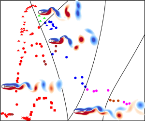
  $m^*$. Figure 4 shows typical vorticity fields, at the time instant of maximum upward deflection, corresponding to the different vortex shedding patterns for points marked in figure 3(b) with letters a to e. Computations have been carried out with three initial conditions: (i) increment in
  $U^*$, (ii) decrement in
  $U^*$ and (iii) flow past stationary filament. The first two are referred to as increasing- and decreasing-
 $U^*$. The three initial conditions lead to the same state in most cases; the states are marked in figure 3, when they do not.

Figure 3. The  ${\textit {Re}}=150$ flow past a fixed cylinder with a flexible filament: variation of (a) dominant frequency
  $F$ and natural frequencies
  $F_k$, (b) r.m.s. displacement
  $A_{rms}$ and (c) average displacement
  $A_{avg}$ of the filament tip with
  $U^*$ for
  $m^*=1,2$ and
  $20$. Pie charts in panel (a) show the contributions of the various EB modes. Blocks below panel (a) show the extent and layout of the branches. Letters L and D refer to lock-in and desynchronization branches. Arrows indicate the increasing- and decreasing-
 $U^*$ initial conditions.

Figure 4. The  ${\textit {Re}}=150$ flow past a fixed cylinder with a flexible filament: instantaneous vorticity fields for
  $(U^*,m^*)=$ (a)
  $(24,2)$, (b)
  $(49,2)$, (c,f)
  $(145,2)$, (d)
  $(80,20)$ and (e)
  $(90,20)$ when the filament tip is at its highest position. The points are indicated in figure 3(b) with letters
  $a$ to
  $e$. Panels (c) and (f) correspond to different time instants for same point on the branch
  $\mathsf{L}_{\mathsf{3i}}$. Type of vortex shedding is also indicated. Vortices shed in one cycle are enclosed in a box.
Multiple lock-ins with different EB modes are observed. The first lock-in occurs with EB-1 on branch  $\mathsf {L}_\mathsf {1}$, as indicated by the proximity of
  $F$ with
  $F_1$ and a peak in
  $A_{rms}$. The pie charts for
  $q_k$ confirm that the predominant mode of vibration at low
  $U^*$ is EB-1, and the system essentially behaves as a single degree of freedom oscillator. Branch
  $\mathsf {L}_\mathsf {1}$ is flanked on either side by the desynchronization regimes (
 $\mathsf {D}_\mathsf {1}$ and
  $\mathsf {D}_\mathsf {2}$) with relatively small
  $A_{rms}$ and
  $F$ close to
  $St_0$. The response of the filament in this low
  $U^*$ regime is qualitatively similar to the VIV of a rigid cylinder and the mode of vortex shedding is 2S.
It is found that the larger the value of  $m^*$, the closer
  $F$ is to
  $F_1$ on branch
  $\mathsf {L}_\mathsf {1}$. This behaviour can be attributed to the reduction in added mass coefficient with increase in
  $m^*$ (Navrose & Mittal Reference Navrose and Mittal2017). Although the peak amplitude is independent of
  $m^*$, it occurs at a higher
  $U^*$ with increase in
  $m^*$. These observations are consistent with VIV of rigid bodies (Sahu et al. Reference Sahu, Furquan, Jaiswal and Mittal2019a). A notable feature of the
  $\mathsf {D}_\mathsf {2}$ branch is symmetry-breaking bifurcation, wherein the mean position of the tip is biased, for low
  $m^*$. A similar symmetry-breaking bifurcation has been reported in the steady solutions by Bagheri, Mazzino & Bottaro (Reference Bagheri, Mazzino and Bottaro2012). In the unsteady case, the steady bias solution serves as the base solution for the unsteady Hopf bifurcation (Pfister & Marquet Reference Pfister and Marquet2020).
Higher modes become active at larger  $U^*$ for the flexible structure. Unlike a rigid body, where further increase in
  $U^*$ does not bring any qualitative change in response once the second desynchronization regime sets in, the response of the flexible filament shifts from branch
  $\mathsf {D}_\mathsf {2}$ to
  $\mathsf {L}_\mathsf {2}$ with increase in
  $U^*$. The shift occurs via an abrupt change in the amplitude as well as frequency of oscillation. The transition between
  $\mathsf {D}_\mathsf {2}$ and
  $\mathsf {L}_\mathsf {2}$ is hysteretic, that is, the response of the system depends on increasing- vs decreasing-
 $U^*$. Branch
  $\mathsf {L}_\mathsf {2}$ is characterized by a significant contribution from the second, besides the first, EB mode as seen from the increase in value of
  $q_2$. Further, the dominant frequency of oscillations follows the
  $F_2$ curve. The amplitude increases significantly with increase in
  $U^*$ before waning off.
Branches  $\mathsf {L}_\mathsf {3}$ and
  $\mathsf {L}_\mathsf {4}$ are characterized by significant values of
  $q_3$ and
  $q_4$. Similar to
  $\mathsf {L}_\mathsf {2}$, the onset of
  $\mathsf {L}_\mathsf {3}$ is also hysteretic. Computations initiated with flow past a stationary filament, for large
  $m^*$ and certain range of
  $U^*$, lead to branches
  $\mathsf {L}^\mathsf {0}_\mathsf {3}$,
  $\mathsf {L}^\mathsf {0}_\mathsf {4}$ and
  $\mathsf {D}_\mathsf {3}$. These states/branches are not approachable from
  $\mathsf {L}_\mathsf {2}$. The response on branches
  $\mathsf {L}^\mathsf {0}_\mathsf {3}$ and
  $\mathsf {L}^\mathsf {0}_\mathsf {4}$ are dominated by the EB-3 and EB-4 modes, respectively. However, unlike other lock-in branches, the amplitude of vibration is smaller and with a significant bias in the mean position. The effect of
  $m^*$ on the lock-in with EB modes is interesting. The contribution of EB-2 decreases on branch
  $\mathsf {L}_\mathsf {2}$ with increase in
  $U^*$ for low
  $m^*$ (
 $=1$ and
  $2$). The behaviour of
  $q_3$ on branch
  $\mathsf {L}_\mathsf {3}$ is similar.
3.2. Physics of vortex shedding
Figures 3 and 4 highlight the large number of modes of vortex shedding that are observed in the free vibration of the flexible filament in the parameter space considered. Contrary to expectation, the vortex-shedding pattern is not sustained on a response branch. For example, three distinct vortex-shedding patterns are observed on  $\mathsf {L}_\mathsf {2}$, namely 2S, 2P and
  $\mathsf {2P+2S}$. In general, 2S mode is observed at the lower
  $U^*$ end of a branch (figure 4a,b), while the more complex 2P,
  $\mathsf {P+S}$ and
  $\mathsf {2P+2S}$ modes occur at higher
  $U^*$. This can be explained by looking at the variation of the vortex-shedding frequency, which is equal to
  $F$, over a branch. It decreases with increase in
  $U^*$ resulting in stretching of the shed vortices as shown in figure 4(b). Eventually for
  $F\lesssim 0.1$, the stretched vortices split into two, resulting in a transition to the 2P mode (figure 4c). Four vortices are shed in one cycle of 2P mode, two of the same sign from each side. A further decrease in frequency leads to an even larger stretching of vortices. When
  $F$ reduces to below 0.07 approximately, the stretched vortices undergo yet another split leading to a transition from the 2P to
  $\mathsf {2P+2S}$ mode of shedding (figure 4e). Such low values of
  $F$ occur only for large
  $m^*$ (figure 4e). In the
  $\mathsf {2P+2S}$ shedding pattern, an additional single vortex, of opposite sign, accompanies the pair of vortices seen in
  $\mathsf{2P}$ mode (Williamson & Roshko Reference Williamson and Roshko1988). The shedding pattern reverts back to 2S mode towards the higher
  $U^*$ end of
  $\mathsf {L}_\mathsf {2}$ with irregular spacing between the vortices. Unlike in VIV of rigid bodies (Mathai et al. Reference Mathai, Zhu, Sun and Lohse2017), the transitions between the vortex-shedding modes on the
  $\mathsf {L}_\mathsf {2}$ branch are not abrupt; rather they occur through a range of intermediate mixed states. While the mode of vortex shedding on
  $\mathsf {L}_\mathsf {3}$,
  $\mathsf {L}_\mathsf {4}$,
  $\mathsf {L}_\mathsf {3}^\mathsf {0}$ and
  $\mathsf {L}_\mathsf {4}^\mathsf {0}$ is 2S, intermittent switching between the 2P and
  $\mathsf {P+S}$ modes of shedding occurs on branch
  $\mathsf {L}_{\mathsf {3i}}$. Three vortices, two of the same sign, are shed in one cycle in the
  $\mathsf {P+S}$ pattern (figure 4f). Intermittency reduces as
  $U^*$ increases and eventually only the 2P mode is observed. It may be noted that the 2S mode is associated with both low and high amplitudes of vibration. However, the modes in which a larger number of vortices are shed in each cycle of oscillation appear only during lock-in when the filament vibrates with relatively large amplitude. The foregoing discussion suggests that the pattern of vortex shedding observed is largely dependent on the amplitude and frequency, irrespective of
  $U^*$ and the associated branch. Williamson & Roshko (Reference Williamson and Roshko1988) identified the regimes of various modes of vortex shedding for the forced vibration of a rigid cylinder on amplitude vs
  $St_0/F$ plane. Their experiments were conducted at relatively large
  ${\textit {Re}}$. We extend their analysis to the present case of flexible filament. We replace the amplitude and frequency of forced vibration with the r.m.s. displacement and frequency of the tip of the flexible filament undergoing free vibration. The map so generated is presented in figure 5. Remarkably, it not only shows clustering of modes into distinct regions but is even qualitatively similar to the one presented in Williamson & Roshko (Reference Williamson and Roshko1988) for the rigid cylinder despite the two VIV systems being very different. This similarity may be attributed to the dependence of the vortex-shedding patterns on the wake itself and not on how the wake is generated. Figure 5 also shows that the mode shapes are relatively insignificant, compared with the tip displacement of the filament, in terms of vortex-shedding patterns. An interesting observation from figure 5 is that the extent of
  $\mathsf {2P+2S}$ does not share a boundary with the 2S mode. Therefore, the transition from the 2S to
  $\mathsf {2P+2S}$ mode is via 2P. We also note that both 2P and 2S modes are possible when the filament vibration frequency is less than 60 per cent of
  $St_0$ approximately. Which of these, 2P or 2S, is actually observed is decided by the amplitude of vibration. Unless the frequency is very low, the 2S mode is preferred for low amplitude as it is associated with a relatively narrower wake. The 2P mode results from stretching of vortices, which requires either a sufficiently low vibration frequency or a wide wake, that results from large amplitude vibration.

Figure 5. The  ${\textit {Re}}=150$ flow past a fixed cylinder with a flexible filament: distribution of vortex shedding modes in the
  $A_{rms}$–
 $St_0/F$ plane for
  $m^*=1,2$ and
  $20$.
$20$.
3.3. Energy transfer between fluid and filament
Kumar, Navrose & Mittal (Reference Kumar, Navrose and Mittal2016) investigated the energy transfer between a rigid cylinder and fluid during VIV. Unlike a rigid body undergoing VIV, a flexible body can gain energy at one location, while simultaneously loosing some of it at another. It is, therefore, possible to locate points on the structure that absorb energy for most part of a cycle, while loosing only a small fraction of it during the remaining. This is despite the fact that no net energy is transferred to the entire structure in one complete cycle when the structural damping is zero. Popular designs for energy harvesting devices use piezo-electric or electromagnetic transducers at certain locations on the body. Identification of ‘maximum energy absorption points’ can be useful in the optimal placement of transducers.
Energy transfer rate (per unit length),  $P(X,t)$, at a location
  $X$ along the filament and instant
  $t$ is defined as follows:
  $P(X,t) = v_n(X,t)\left[\kern-0.15em\left[ {p(X,t)} \right]\kern-0.15em\right]$, where
  $v_n(X,t)$ and
  $\left[\kern-0.15em\left[ {p(X,t)} \right]\kern-0.15em\right]$ respectively denote the normal component of filament velocity and difference between pressure on the two sides. The viscous forces contribute negligibly to the energy budget and are not included in the estimate. Figure 6 shows contours of
  $P(X,t)$ with
  $(X,t) \in [0,L]\times [\tau ,\tau +T]$, for selected points marked with letters A to H in figure 3(b). A positive value of
  $P$ corresponds to gain in energy of the filament. The topology of the contours is mainly governed by the underlying dominant EB mode. Cases dominated by the first EB-1 mode (A,D,E,F), show only one sink (red spot) in a half-cycle. Similarly, those dominated by the second mode (C,G) and by the fourth mode (H) respectively show two and four such spots. This pattern is consistent with the number of antinodes in the corresponding modes. Most energy contours have a period of
  $T/2$. However, the contours for two halves of the single cycle are different for B and H due to bias in the mean position of the filament.

Figure 6. The  ${\textit {Re}}=150$ flow past a fixed cylinder with a flexible filament: space–time contours showing energy (per unit length) transfer rate across the length of the filament during one cycle of oscillation at points marked using letters A to H in figure 3.
As expected, maximum value of  $P$ is higher when
  $A_{rms}$ is large (D,E,F and G). Maximum energy absorption is along
  $\mathsf {L}_\mathsf {2}$,
  $\mathsf {L}_\mathsf {3}$ and
  $\mathsf {L}_\mathsf {4}$ branches. It is higher for
  $U^*\gtrsim 30$ and low
  $m^*$. Further, the maximum value of energy transfer rate,
  $P_{max}$, for most cases is located at
  $X\sim 2.5\text {--}3$. This, therefore, is the best location for placing transducers to extract energy. However, response of a real device will be affected by the presence of a transducer as well. The recommendations made here are suggestive, aimed towards narrowing down the already vast parameter space.
4. Conclusions
We have identified, by investigating a wide range of inertia and flexibility, lock-in branches corresponding to the first four EB modes in the response of a flexible filament behind a cylinder. Response of the filament shifts abruptly, and hysteretically, from one branch to another as  $U^*$ is varied. Each such transition is accompanied by a sharp change in the contribution of a particular EB mode. Increasing inertia of the filament brings its frequency closer to the natural frequency during lock-in. There is no fixed vortex-shedding pattern for a branch, rather the frequency and amplitude of a state decide the type of pattern observed. While the simpler 2S pattern is observed at higher frequencies, one of the more complex 2P,
  $\mathsf {P+S}$ and
  $\mathsf {2P+2S}$ patterns gets selected, based on the value of amplitude, at lower frequencies. Using r.m.s. amplitude and the dominant frequency of the tip vibration, we have generalized the delimitation of vortex-shedding modes in the amplitude–frequency plane from forced vibration of a cylinder (Williamson & Roshko Reference Williamson and Roshko1988) to the present case. That the vortex-shedding map for rigid and flexible bodies have strong similarities, suggests that it might be possible to construct a universal map valid for all wakes irrespective of the geometric complexity of the body. The spatio-temporal distribution of energy transfer primarily depends on the dominant EB mode. Maximum gain in energy of the filament takes place at approximately 70 %–85 % of its length from the base and its value correlates well with the amplitude of vibration.
Acknowledgements
The authors are grateful to Dr Navrose, Department of Aerospace Engineering, IIT Kanpur, for his insights into energy exchange between fluid and structure. All computations were performed using the High Performance Computing facility at the Indian Institute of Technology Kanpur, set up under the aegis of the Department of Science and Technology (DST), India. We also acknowledge the help from T. Ram Sahu, G. Chopra and A. Desai in carrying out some of the computations.
Declaration of interests
The authors report no conflict of interest.


