


1 Introduction
Granular flows have been widely studied in recent years because of their importance in industrial processes and geophysical flows such as avalanches, debris or rock avalanches, landslides, etc. In particular, numerical modelling of geophysical granular flows provides a unique tool for hazard assessment.
The behaviour of real geophysical flows is very complex due to topography effects, the heterogeneity of the material involved, the presence of fluid phases, fragmentation, etc. (Delannay et al.
Reference Delannay, Valance, Mangeney, Roche and Richard2015). One of the major issues is to quantify erosion/deposition processes that play a key role in geophysical flow dynamics but are very difficult to measure in the field (see e.g. Conway et al.
Reference Conway, Decaulne, Balme, Murray and Towner2010; Berger, McArdell & Schlunegger Reference Berger, McArdell and Schlunegger2011; Iverson et al.
Reference Iverson, Reid, Logan, LaHusen, Godt and Griswold2011). Laboratory experiments on granular flows are very useful to test flow models on simple configurations where detailed measurements can be performed, even if some physical processes may differ between the large and small scale. These experiments may help in defining appropriate rheological laws to describe the behaviour of granular materials. Recent experiments by Mangeney et al. (Reference Mangeney, Roche, Hungr, Mangold, Faccanoni and Lucas2010) and Farin, Mangeney & Roche (Reference Farin, Mangeney and Roche2014) on granular column collapse have quantified how the dynamics and deposits of dry granular flows change in the presence of an erodible bed. They showed a significant increase of the runout distance (i.e. maximum distance reached by the deposit) and flow duration with increasing thickness of the erodible bed. This strong effect of bed entrainment was observed only for flows on slopes higher than a critical angle of approximately
 $16^{\circ }$
for glass beads. The question remains as to whether this behaviour can be reproduced by granular flow models.
$16^{\circ }$
for glass beads. The question remains as to whether this behaviour can be reproduced by granular flow models.
Understanding the rheological behaviour of granular material is a major challenge. In particular, a key issue is to describe the transition between flow (fluid-like) and no-flow (solid-like) behaviour. Granular flows have been described by viscoplastic laws and especially by the so-called
 ${\it\mu}(I)$
-rheology, introduced by Jop, Forterre & Pouliquen (Reference Jop, Forterre and Pouliquen2006). It specifies that the friction coefficient
${\it\mu}(I)$
-rheology, introduced by Jop, Forterre & Pouliquen (Reference Jop, Forterre and Pouliquen2006). It specifies that the friction coefficient
 ${\it\mu}$
is variable and depends on the inertial number
${\it\mu}$
is variable and depends on the inertial number
 $I$
that is related to the pressure and strain rate. Jop, Forterre & Pouliquen (Reference Jop, Forterre and Pouliquen2007) considered this viscoplastic law and compared their results with laboratory experiments to investigate the time evolution of the vertical profile of velocity in narrow channels, where the sidewall friction is modelled through an additional friction term introduced by Jop, Forterre & Pouliquen (Reference Jop, Forterre and Pouliquen2005). Lagrée, Staron & Popinet (Reference Lagrée, Staron and Popinet2011) implemented the
$I$
that is related to the pressure and strain rate. Jop, Forterre & Pouliquen (Reference Jop, Forterre and Pouliquen2007) considered this viscoplastic law and compared their results with laboratory experiments to investigate the time evolution of the vertical profile of velocity in narrow channels, where the sidewall friction is modelled through an additional friction term introduced by Jop, Forterre & Pouliquen (Reference Jop, Forterre and Pouliquen2005). Lagrée, Staron & Popinet (Reference Lagrée, Staron and Popinet2011) implemented the
 ${\it\mu}(I)$
-rheology in a full Navier–Stokes solver (Gerris) by defining a viscosity from the
${\it\mu}(I)$
-rheology in a full Navier–Stokes solver (Gerris) by defining a viscosity from the
 ${\it\mu}(I)$
-rheology. They validated the model with two-dimensional (2D) analytical solutions and compared it to 2D discrete element simulations of granular collapses over horizontal rigid beds and with other rheologies. Staron, Lagrée & Popinet (Reference Staron, Lagrée and Popinet2012) and Staron, Lagrée & Popinet (Reference Staron, Lagrée and Popinet2014) applied this model to granular flows in a silo. Using an augmented Lagrangian method combined with finite element discretisation to solve the 2D full Navier–Stokes equations, Ionescu et al. (Reference Ionescu, Mangeney, Bouchut and Roche2015) showed that this rheology quantitatively reproduces laboratory experiments of granular collapses over horizontal and inclined planes. By interpreting the
${\it\mu}(I)$
-rheology. They validated the model with two-dimensional (2D) analytical solutions and compared it to 2D discrete element simulations of granular collapses over horizontal rigid beds and with other rheologies. Staron, Lagrée & Popinet (Reference Staron, Lagrée and Popinet2012) and Staron, Lagrée & Popinet (Reference Staron, Lagrée and Popinet2014) applied this model to granular flows in a silo. Using an augmented Lagrangian method combined with finite element discretisation to solve the 2D full Navier–Stokes equations, Ionescu et al. (Reference Ionescu, Mangeney, Bouchut and Roche2015) showed that this rheology quantitatively reproduces laboratory experiments of granular collapses over horizontal and inclined planes. By interpreting the
 ${\it\mu}(I)$
-rheology as a viscoplastic flow with a Drucker–Prager yield stress criterion and a viscosity depending on the pressure and strain rate, they showed that the mean value of this viscosity has a key impact on the simulated front dynamics and on the deposit of granular column collapses. In particular without viscosity, the runout distance is strongly overestimated. However, using a constant viscosity or a spatio-temporally variable viscosity only slightly changes the results for granular columns of small aspect ratio (see Ionescu et al.
Reference Ionescu, Mangeney, Bouchut and Roche2015).
${\it\mu}(I)$
-rheology as a viscoplastic flow with a Drucker–Prager yield stress criterion and a viscosity depending on the pressure and strain rate, they showed that the mean value of this viscosity has a key impact on the simulated front dynamics and on the deposit of granular column collapses. In particular without viscosity, the runout distance is strongly overestimated. However, using a constant viscosity or a spatio-temporally variable viscosity only slightly changes the results for granular columns of small aspect ratio (see Ionescu et al.
Reference Ionescu, Mangeney, Bouchut and Roche2015).
In Chauchat & Médale (Reference Chauchat and Médale2014), the authors implemented the
 ${\it\mu}(I)$
-rheology in a three-dimensional numerical model with a finite element method combined with the Newton–Raphson algorithm with a regularization technique. The numerical model was validated by an analytical solution for a dry granular vertical-chute flow and a dry granular flow over an inclined plane and by laboratory experiments. Previously, Chauchat & Médale (Reference Chauchat and Médale2010) simulated the bed-load transport problem in 2D and 3D with a two-phase model that considers a Drucker–Prager rheology for the granular phase. Lusso et al. (Reference Lusso, Ern, Bouchut, Mangeney, Farin and Roche2015b
) used a finite element method to simulate a 2D viscoplastic flow considering a Drucker–Prager yield stress criterion and a constant viscosity. They obtained similar results taking into account either a regularization method or the augmented Lagrangian algorithm. By comparing the simulated normal velocity profiles and the time change of the position of the flow/no-flow (i.e. flowing/static) interface with laboratory experiments by Farin et al. (Reference Farin, Mangeney and Roche2014), they concluded that a pressure and rate-dependent viscosity can be important to study flows over an erodible bed. A similar conclusion is presented in Lusso et al. (Reference Lusso, Bouchut, Ern and Mangeney2015a
) after comparing the normal velocity profiles and the position of the flow/no-flow interface during the stopping phase of granular flows over erodible beds calculated with a simplified thin-layer but not depth-averaged viscoplastic model (Bouchut, Ionescu & Mangeney Reference Bouchut, Ionescu and Mangeney2016) with those measured in laboratory experiments.
${\it\mu}(I)$
-rheology in a three-dimensional numerical model with a finite element method combined with the Newton–Raphson algorithm with a regularization technique. The numerical model was validated by an analytical solution for a dry granular vertical-chute flow and a dry granular flow over an inclined plane and by laboratory experiments. Previously, Chauchat & Médale (Reference Chauchat and Médale2010) simulated the bed-load transport problem in 2D and 3D with a two-phase model that considers a Drucker–Prager rheology for the granular phase. Lusso et al. (Reference Lusso, Ern, Bouchut, Mangeney, Farin and Roche2015b
) used a finite element method to simulate a 2D viscoplastic flow considering a Drucker–Prager yield stress criterion and a constant viscosity. They obtained similar results taking into account either a regularization method or the augmented Lagrangian algorithm. By comparing the simulated normal velocity profiles and the time change of the position of the flow/no-flow (i.e. flowing/static) interface with laboratory experiments by Farin et al. (Reference Farin, Mangeney and Roche2014), they concluded that a pressure and rate-dependent viscosity can be important to study flows over an erodible bed. A similar conclusion is presented in Lusso et al. (Reference Lusso, Bouchut, Ern and Mangeney2015a
) after comparing the normal velocity profiles and the position of the flow/no-flow interface during the stopping phase of granular flows over erodible beds calculated with a simplified thin-layer but not depth-averaged viscoplastic model (Bouchut, Ionescu & Mangeney Reference Bouchut, Ionescu and Mangeney2016) with those measured in laboratory experiments.
Because of the high computational cost of solving the full 3D Navier–Stokes equations, in particular in a geophysical context, granular flows have often been simulated using depth-averaged shallow models. The shallow or thin-layer approximation (the thickness of the flow is assumed to be small compared to its downslope extension) associated with depth-averaging leads to conservation laws like the Saint-Venant equations. These approximations have been applied to granular flows by Savage & Hutter (Reference Savage and Hutter1989) by assuming a Coulomb friction law where the shear stress at the bottom is proportional to the normal stress, with a constant friction coefficient
 ${\it\mu}$
. However, this model does not reproduce the increase in runout distance observed with increasing thickness of the erodible bed. The analytical solution deduced in Faccanoni & Mangeney (Reference Faccanoni and Mangeney2013) proves that this model leads to the opposite effect. The question is as to whether this opposite behaviour between the experiments and simulations is due to the thin-layer approximation and/or depth-averaging process or to the rheological law implemented in the model (i.e. constant friction coefficient).
${\it\mu}$
. However, this model does not reproduce the increase in runout distance observed with increasing thickness of the erodible bed. The analytical solution deduced in Faccanoni & Mangeney (Reference Faccanoni and Mangeney2013) proves that this model leads to the opposite effect. The question is as to whether this opposite behaviour between the experiments and simulations is due to the thin-layer approximation and/or depth-averaging process or to the rheological law implemented in the model (i.e. constant friction coefficient).
Recently, Capart, Hung & Stark (Reference Capart, Hung and Stark2015) proposed a depth-integrated model taking into account a linearization of the
 ${\it\mu}(I)$
-rheology. They prescribed an S-shaped velocity profile corresponding to equilibrium debris flows and typical of granular flows over erodible beds. Their velocity profiles were reconstructed using the computed averaged velocity making it possible to compare their results with velocity profiles measured in laboratory experiments. Gray & Edwards (Reference Gray and Edwards2014) introduced the
${\it\mu}(I)$
-rheology. They prescribed an S-shaped velocity profile corresponding to equilibrium debris flows and typical of granular flows over erodible beds. Their velocity profiles were reconstructed using the computed averaged velocity making it possible to compare their results with velocity profiles measured in laboratory experiments. Gray & Edwards (Reference Gray and Edwards2014) introduced the
 ${\it\mu}(I)$
-rheology in a depth-averaged model by adding a viscous term and prescribing a Bagnold velocity profile, typical of granular flows over rigid beds. Edwards & Gray (Reference Edwards and Gray2015) showed the ability of this model to capture roll-waves and erosion-deposition waves, if it is combined with the basal friction law introduced in Pouliquen & Forterre (Reference Pouliquen and Forterre2002). In these two depth-averaged models, however, the shape of the velocity profile is prescribed so that they cannot reproduce the different profiles observed in highly transient flows such as in granular collapses where the velocity profiles change from Bagnold-like near the front to S-shaped upstream where upper grains flow above static grains (see Ionescu et al.
Reference Ionescu, Mangeney, Bouchut and Roche2015). Furthermore, in depth-averaged models, only the mean velocity over the whole thickness of the flow is calculated (i.e., the whole granular column is either flowing or at rest, except for the model proposed by Capart et al. (Reference Capart, Hung and Stark2015)). Granular collapse experiments and simulations have shown on the contrary that during the stopping phase and when erosion/deposition processes occur, static zones may develop near the bottom and propagate upwards. The resulting normal gradient of the downslope velocity, which changes in time, is a significant term in the strain rate and therefore strongly influences the
${\it\mu}(I)$
-rheology in a depth-averaged model by adding a viscous term and prescribing a Bagnold velocity profile, typical of granular flows over rigid beds. Edwards & Gray (Reference Edwards and Gray2015) showed the ability of this model to capture roll-waves and erosion-deposition waves, if it is combined with the basal friction law introduced in Pouliquen & Forterre (Reference Pouliquen and Forterre2002). In these two depth-averaged models, however, the shape of the velocity profile is prescribed so that they cannot reproduce the different profiles observed in highly transient flows such as in granular collapses where the velocity profiles change from Bagnold-like near the front to S-shaped upstream where upper grains flow above static grains (see Ionescu et al.
Reference Ionescu, Mangeney, Bouchut and Roche2015). Furthermore, in depth-averaged models, only the mean velocity over the whole thickness of the flow is calculated (i.e., the whole granular column is either flowing or at rest, except for the model proposed by Capart et al. (Reference Capart, Hung and Stark2015)). Granular collapse experiments and simulations have shown on the contrary that during the stopping phase and when erosion/deposition processes occur, static zones may develop near the bottom and propagate upwards. The resulting normal gradient of the downslope velocity, which changes in time, is a significant term in the strain rate and therefore strongly influences the
 ${\it\mu}(I)$
coefficient. The well-posedness of the full
${\it\mu}(I)$
coefficient. The well-posedness of the full
 ${\it\mu}(I)$
-rheology is proved by Barker et al. (Reference Barker, Schaeffer, Bohorquez and Gray2015) for a large intermediate range of values of the inertial number
${\it\mu}(I)$
-rheology is proved by Barker et al. (Reference Barker, Schaeffer, Bohorquez and Gray2015) for a large intermediate range of values of the inertial number
 $I$
. It is ill-posed for low and high values of
$I$
. It is ill-posed for low and high values of
 $I$
, even for steady-uniform flows where
$I$
, even for steady-uniform flows where
 $I$
ranges from zero to infinity when the slope varies between the limit angles of the
$I$
ranges from zero to infinity when the slope varies between the limit angles of the
 ${\it\mu}(I)$
-rheology.
${\it\mu}(I)$
-rheology.
Multilayer models represent an interesting alternative to depth-averaged models, making it possible in particular to resolve the shape of velocity profiles. They were introduced by Audusse (Reference Audusse2005) and extended by Audusse, Bristeau & Decoene (Reference Audusse, Bristeau and Decoene2008). A different multilayer model, which takes into account the exchange of mass and momentum between the layers, has since been derived by Audusse et al. (Reference Audusse, Bristeau, Perthame and Sainte-Marie2011a ,Reference Audusse, Bristeau, Pelanti and Sainte-Marie b ), and Sainte-Marie (Reference Sainte-Marie2011).
A new procedure to obtain a multilayer model has been introduced by Fernández-Nieto, Koné & Chacón Rebollo (Reference Fernández-Nieto, Koné and Chacón Rebollo2014). Several differences appear between this multilayer model and the ones deduced by Audusse et al. First, in Fernández-Nieto et al. (Reference Fernández-Nieto, Koné and Chacón Rebollo2014), the multilayer model is derived from the variational formulation of Navier–Stokes equations with hydrostatic pressure by considering a discontinuous profile of the solution at the interfaces of a vertical partition of the domain. This procedure proves that the solution of this multilayer model is a particular weak solution of the Navier–Stokes system. Moreover, the mass and momentum transfer terms at the interfaces of the normal partition are deduced from the jump conditions verified by the weak solutions of the Navier–Stokes system. In addition, the definition of the vertical velocity profile is easily obtained using the mass jump condition combined with the incompressibility condition.
By comparing this model with granular flow experiments on erodible beds (Jop et al.
Reference Jop, Forterre and Pouliquen2007; Mangeney et al.
Reference Mangeney, Roche, Hungr, Mangold, Faccanoni and Lucas2010; Farin et al.
Reference Farin, Mangeney and Roche2014), we evaluate (i) if the model with the
 ${\it\mu}(I)$
-rheology gives a reasonable approximation of the granular flow dynamics in different regimes and of their deposits, (ii) if the model is able to reproduce strong changes in velocity profiles during highly transient flows, (iii) if it reproduces the increase in runout distance observed for granular collapses for increasing thickness of the erodible bed above a critical slope angle
${\it\mu}(I)$
-rheology gives a reasonable approximation of the granular flow dynamics in different regimes and of their deposits, (ii) if the model is able to reproduce strong changes in velocity profiles during highly transient flows, (iii) if it reproduces the increase in runout distance observed for granular collapses for increasing thickness of the erodible bed above a critical slope angle
 ${\it\theta}_{c}\in [12^{\circ },16^{\circ }]$
and (iv) how the multilayer approach improves the results compared to the classical depth-averaged Saint-Venant model (i.e. monolayer model).
${\it\theta}_{c}\in [12^{\circ },16^{\circ }]$
and (iv) how the multilayer approach improves the results compared to the classical depth-averaged Saint-Venant model (i.e. monolayer model).
The paper is organised as follows. Section 2 is devoted to presenting the initial system composed of the 2D Navier–Stokes equations with the
 ${\it\mu}(I)$
-rheology and the appropriate boundary conditions. We also give the local coordinates system that we consider for the derivation. In § 3 we present the multilayer approach following Fernández-Nieto et al. (Reference Fernández-Nieto, Koné and Chacón Rebollo2014) to derive a 2D multilayer model for dry granular flows up to first order when considering the thin-layer asymptotic approximation. The final
${\it\mu}(I)$
-rheology and the appropriate boundary conditions. We also give the local coordinates system that we consider for the derivation. In § 3 we present the multilayer approach following Fernández-Nieto et al. (Reference Fernández-Nieto, Koné and Chacón Rebollo2014) to derive a 2D multilayer model for dry granular flows up to first order when considering the thin-layer asymptotic approximation. The final
 ${\it\mu}(I)$
-rheology multilayer shallow model (MSM) is also presented in this section together with the associated energy balance. Section 4 is devoted to presenting the numerical results. First, we validate our model using the 2D analytical solution of a Bagnold flow and a flow in a narrow channel with a strong effect from the lateral wall friction. We also compare with experimental data for the previous case, and do a deeper comparison of our results with granular collapse laboratory experiments done by Mangeney et al. (Reference Mangeney, Roche, Hungr, Mangold, Faccanoni and Lucas2010). We show that the
${\it\mu}(I)$
-rheology multilayer shallow model (MSM) is also presented in this section together with the associated energy balance. Section 4 is devoted to presenting the numerical results. First, we validate our model using the 2D analytical solution of a Bagnold flow and a flow in a narrow channel with a strong effect from the lateral wall friction. We also compare with experimental data for the previous case, and do a deeper comparison of our results with granular collapse laboratory experiments done by Mangeney et al. (Reference Mangeney, Roche, Hungr, Mangold, Faccanoni and Lucas2010). We show that the
 ${\it\mu}(I)$
-rheology is able to qualitatively reproduce the increase in runout distance of granular flows over erodible beds, in contrast with the constant friction model. Moreover, the multilayer approach reproduces the change in shape of the velocity profiles and significantly improves results compared to the monolayer one (i.e. Saint-Venant). Finally, conclusions are presented in § 5.
${\it\mu}(I)$
-rheology is able to qualitatively reproduce the increase in runout distance of granular flows over erodible beds, in contrast with the constant friction model. Moreover, the multilayer approach reproduces the change in shape of the velocity profiles and significantly improves results compared to the monolayer one (i.e. Saint-Venant). Finally, conclusions are presented in § 5.
2 The initial system
In this section we present the two-dimensional model considered to describe the dynamics of granular flows. First, we introduce the starting system of equations, completed with the definition of the stress tensor including the
 ${\it\mu}(I)$
-rheology. We then specify the suitable boundary conditions. Finally, we present the complete model in local coordinates.
${\it\mu}(I)$
-rheology. We then specify the suitable boundary conditions. Finally, we present the complete model in local coordinates.
2.1 Governing equations
We consider a granular mass flow with velocity
 $\boldsymbol{u}\in \mathbb{R}^{2}$
and density
$\boldsymbol{u}\in \mathbb{R}^{2}$
and density
 ${\it\rho}\in \mathbb{R}$
and we set the incompressible Navier–Stokes equations describing the dynamics of the system:
${\it\rho}\in \mathbb{R}$
and we set the incompressible Navier–Stokes equations describing the dynamics of the system:
 $$\begin{eqnarray}\left.\begin{array}{@{}c@{}}\displaystyle \boldsymbol{{\rm\nabla}}\boldsymbol{\cdot }\boldsymbol{u}=0,\\ \displaystyle {\it\rho}\partial _{t}\boldsymbol{u}+{\it\rho}\boldsymbol{{\rm\nabla}}\boldsymbol{\cdot }(\boldsymbol{u}\otimes \boldsymbol{u})-\boldsymbol{{\rm\nabla}}\boldsymbol{\cdot }{\bf\sigma}={\it\rho}\boldsymbol{g},\end{array}\right\}\end{eqnarray}$$
where
 $\boldsymbol{g}$
is the gravity force. The total stress tensor is
$\boldsymbol{g}$
is the gravity force. The total stress tensor is
 $$\begin{eqnarray}{\bf\sigma}=-p\unicode[STIX]{x1D644}+{\bf\tau},\end{eqnarray}$$
with
 $p\in \mathbb{R}$
the pressure.
$p\in \mathbb{R}$
the pressure.
 $\unicode[STIX]{x1D644}$
is the 2D identity tensor and
$\unicode[STIX]{x1D644}$
is the 2D identity tensor and
 ${\bf\tau}$
the deviatoric stress tensor given by
${\bf\tau}$
the deviatoric stress tensor given by
 $$\begin{eqnarray}{\bf\tau}={\it\eta}\unicode[STIX]{x1D63F}(\boldsymbol{u}),\end{eqnarray}$$
where
 ${\it\eta}\in \mathbb{R}$
denotes the viscosity and
${\it\eta}\in \mathbb{R}$
denotes the viscosity and
 $\unicode[STIX]{x1D63F}(\boldsymbol{u})$
the strain-rate tensor
$\unicode[STIX]{x1D63F}(\boldsymbol{u})$
the strain-rate tensor
 $$\begin{eqnarray}\unicode[STIX]{x1D63F}(\boldsymbol{u})={\textstyle \frac{1}{2}}(\boldsymbol{{\rm\nabla}}\boldsymbol{u}+(\boldsymbol{{\rm\nabla}}\boldsymbol{u})^{\prime }).\end{eqnarray}$$
2.2
 ${\it\mu}(I)$
-rheology
${\it\mu}(I)$
-rheology

As discussed in the Introduction, we consider the so-called
 ${\it\mu}(I)$
-rheology (see Jop et al.
Reference Jop, Forterre and Pouliquen2006) in order to take into account the non-Newtonian nature of granular flows. Hence, the viscosity coefficient is defined by
${\it\mu}(I)$
-rheology (see Jop et al.
Reference Jop, Forterre and Pouliquen2006) in order to take into account the non-Newtonian nature of granular flows. Hence, the viscosity coefficient is defined by
 $$\begin{eqnarray}{\it\eta}=\frac{{\it\mu}(I)p}{\Vert \unicode[STIX]{x1D63F}(\boldsymbol{u})\Vert },\end{eqnarray}$$
with
 $\Vert \unicode[STIX]{x1D63F}\Vert =\sqrt{0.5\;\unicode[STIX]{x1D63F}\boldsymbol{ :}\unicode[STIX]{x1D63F}}$
the usual second invariant of a tensor
$\Vert \unicode[STIX]{x1D63F}\Vert =\sqrt{0.5\;\unicode[STIX]{x1D63F}\boldsymbol{ :}\unicode[STIX]{x1D63F}}$
the usual second invariant of a tensor
 $\unicode[STIX]{x1D63F}$
. The friction coefficient
$\unicode[STIX]{x1D63F}$
. The friction coefficient
 ${\it\mu}(I)$
is written as
${\it\mu}(I)$
is written as
 $$\begin{eqnarray}{\it\mu}(I)={\it\mu}_{s}+\frac{{\it\mu}_{2}-{\it\mu}_{s}}{I_{0}+I}I,\end{eqnarray}$$
where
 $I_{0}$
is a constant value and
$I_{0}$
is a constant value and
 ${\it\mu}_{2}>{\it\mu}_{s}$
are constant parameters.
${\it\mu}_{2}>{\it\mu}_{s}$
are constant parameters.
 $I$
is the inertial number
$I$
is the inertial number
 $$\begin{eqnarray}I=\frac{2d_{s}\Vert \unicode[STIX]{x1D63F}(\boldsymbol{u})\Vert }{\sqrt{p/{\it\rho}_{s}}},\end{eqnarray}$$
where
 $d_{s}$
is the particle diameter and
$d_{s}$
is the particle diameter and
 ${\it\rho}_{s}$
the particle density. The apparent flow density is then defined as
${\it\rho}_{s}$
the particle density. The apparent flow density is then defined as
 $$\begin{eqnarray}{\it\rho}={\it\varphi}_{s}{\it\rho}_{s},\end{eqnarray}$$
where the solid volume fraction, denoted by
 ${\it\varphi}_{s}$
, is assumed to be constant.
${\it\varphi}_{s}$
, is assumed to be constant.
Note that when the shear rate is equal to zero,
 ${\it\mu}(I)$
is reduced to
${\it\mu}(I)$
is reduced to
 ${\it\mu}_{s}$
. For high values of the inertial number,
${\it\mu}_{s}$
. For high values of the inertial number,
 ${\it\mu}(I)$
converges to
${\it\mu}(I)$
converges to
 ${\it\mu}_{2}$
. Otherwise, if we consider a constant value of
${\it\mu}_{2}$
. Otherwise, if we consider a constant value of
 ${\it\mu}$
, independent of
${\it\mu}$
, independent of
 $I$
, the model is always ill-posed (see Schaeffer Reference Schaeffer1987).
$I$
, the model is always ill-posed (see Schaeffer Reference Schaeffer1987).
The
 ${\it\mu}(I)$
-rheology includes a Drucker–Prager plasticity criterion, the deviatoric tensor is defined as
${\it\mu}(I)$
-rheology includes a Drucker–Prager plasticity criterion, the deviatoric tensor is defined as
 $$\begin{eqnarray}\left.\begin{array}{@{}cc@{}}\displaystyle {\bf\tau}=\frac{{\it\mu}(I)p}{\Vert \unicode[STIX]{x1D63F}\Vert }\,\unicode[STIX]{x1D63F} & \text{if }\Vert \unicode[STIX]{x1D63F}\Vert \neq 0,\\ \displaystyle \Vert {\bf\tau}\Vert \leqslant {\it\mu}_{s}p & \text{if }\Vert \unicode[STIX]{x1D63F}\Vert =0.\end{array}\right\}\end{eqnarray}$$
Note that the
 ${\it\mu}(I)$
-rheology can equivalently be written as a decomposition of the deviatoric stress in a sum of a plastic term and a rate-dependent viscous term (see Ionescu et al.
Reference Ionescu, Mangeney, Bouchut and Roche2015):
${\it\mu}(I)$
-rheology can equivalently be written as a decomposition of the deviatoric stress in a sum of a plastic term and a rate-dependent viscous term (see Ionescu et al.
Reference Ionescu, Mangeney, Bouchut and Roche2015):
 $$\begin{eqnarray}\left.\begin{array}{@{}cc@{}}\displaystyle {\bf\tau}=\frac{{\it\mu}_{s}p}{\Vert \unicode[STIX]{x1D63F}\Vert }\unicode[STIX]{x1D63F}+2\tilde{{\it\eta}}\unicode[STIX]{x1D63F} & \text{if }\Vert \unicode[STIX]{x1D63F}\Vert \neq 0,\\ \displaystyle \Vert {\bf\tau}\Vert \leqslant {\it\mu}_{s}p & \text{if }\Vert \unicode[STIX]{x1D63F}\Vert =0;\end{array}\right\}\end{eqnarray}$$
with a viscosity defined as
 $\tilde{{\it\eta}}=({\it\mu}_{2}-{\it\mu}_{s})p/(I_{0}/d_{s}\sqrt{p/{\it\rho}_{s}}+2\Vert \unicode[STIX]{x1D63F}\Vert )$
. Here we investigate the rheology defined by a variable friction
$\tilde{{\it\eta}}=({\it\mu}_{2}-{\it\mu}_{s})p/(I_{0}/d_{s}\sqrt{p/{\it\rho}_{s}}+2\Vert \unicode[STIX]{x1D63F}\Vert )$
. Here we investigate the rheology defined by a variable friction
 ${\it\mu}(I)$
and a constant friction
${\it\mu}(I)$
and a constant friction
 ${\it\mu}_{s}$
. In Ionescu et al. (Reference Ionescu, Mangeney, Bouchut and Roche2015), the authors showed that simulations of the front propagation of granular column collapses and of their deposits are very sensitive to the value of the average value of the viscosity (see their figures 8 and 13). However, replacing
${\it\mu}_{s}$
. In Ionescu et al. (Reference Ionescu, Mangeney, Bouchut and Roche2015), the authors showed that simulations of the front propagation of granular column collapses and of their deposits are very sensitive to the value of the average value of the viscosity (see their figures 8 and 13). However, replacing
 $\tilde{{\it\eta}}$
by a constant viscosity equal to the averaged value of the spatio-temporal viscosity
$\tilde{{\it\eta}}$
by a constant viscosity equal to the averaged value of the spatio-temporal viscosity
 $\tilde{{\it\eta}}$
does not significantly change the simulated dynamics and deposit. Here we compare the case where
$\tilde{{\it\eta}}$
does not significantly change the simulated dynamics and deposit. Here we compare the case where
 ${\it\mu}={\it\mu}_{s}$
so that
${\it\mu}={\it\mu}_{s}$
so that
 $\tilde{{\it\eta}}=0$
with the
$\tilde{{\it\eta}}=0$
with the
 ${\it\mu}(I)$
rheology corresponding to typical values of the viscosity
${\it\mu}(I)$
rheology corresponding to typical values of the viscosity
 ${\it\eta}=1$
Pa s for granular collapses over horizontal and inclined planes (Ionescu et al.
Reference Ionescu, Mangeney, Bouchut and Roche2015).
${\it\eta}=1$
Pa s for granular collapses over horizontal and inclined planes (Ionescu et al.
Reference Ionescu, Mangeney, Bouchut and Roche2015).
The model considering a viscosity defined by (2.5) presents a discontinuity when
 $\Vert \unicode[STIX]{x1D63F}(\boldsymbol{u})\Vert =0$
. To avoid this singularity there are several ways to proceed. One of them is to apply a duality method, such as augmented Lagrangian methods (Glowinski & Tallec Reference Glowinski and Tallec1989) or the Bermúdez–Moreno algorithm (Bermúdez & Moreno Reference Bermúdez and Moreno1981). Another option is to use a regularization of
$\Vert \unicode[STIX]{x1D63F}(\boldsymbol{u})\Vert =0$
. To avoid this singularity there are several ways to proceed. One of them is to apply a duality method, such as augmented Lagrangian methods (Glowinski & Tallec Reference Glowinski and Tallec1989) or the Bermúdez–Moreno algorithm (Bermúdez & Moreno Reference Bermúdez and Moreno1981). Another option is to use a regularization of
 $\unicode[STIX]{x1D63F}(\boldsymbol{u})$
, which is cheaper computationally; however, it does not give an exact solution, contrary to duality methods.
$\unicode[STIX]{x1D63F}(\boldsymbol{u})$
, which is cheaper computationally; however, it does not give an exact solution, contrary to duality methods.
In this work, we take into consideration two kinds of regularizations of
 $\unicode[STIX]{x1D63F}(\boldsymbol{u})$
. First, we use the regularization proposed in Lagrée et al. (Reference Lagrée, Staron and Popinet2011), which consists of bounding the viscosity by
$\unicode[STIX]{x1D63F}(\boldsymbol{u})$
. First, we use the regularization proposed in Lagrée et al. (Reference Lagrée, Staron and Popinet2011), which consists of bounding the viscosity by
 ${\it\eta}_{M}=250{\it\rho}\sqrt{gh^{3}}$
Pa s, considering instead of (2.5),
${\it\eta}_{M}=250{\it\rho}\sqrt{gh^{3}}$
Pa s, considering instead of (2.5),
 $$\begin{eqnarray}{\it\eta}=\frac{{\it\mu}(I)p}{\max \left(\Vert \unicode[STIX]{x1D63F}(\boldsymbol{u})\Vert ,\displaystyle \frac{{\it\mu}(I)p}{{\it\eta}_{M}}\right)}.\end{eqnarray}$$
In this way, we obtain
 ${\it\eta}={\it\eta}_{M}$
if
${\it\eta}={\it\eta}_{M}$
if
 $\Vert \unicode[STIX]{x1D63F}(\boldsymbol{u})\Vert$
is close to zero. We used this regularization in the simulation of the granular flow experiments. However, as explained in § 4.1.1, we cannot consider this regularization in some tests presented below, for which we have to take into account the regularization introduced in Bercovier & Engelman (Reference Bercovier and Engelman1980),
$\Vert \unicode[STIX]{x1D63F}(\boldsymbol{u})\Vert$
is close to zero. We used this regularization in the simulation of the granular flow experiments. However, as explained in § 4.1.1, we cannot consider this regularization in some tests presented below, for which we have to take into account the regularization introduced in Bercovier & Engelman (Reference Bercovier and Engelman1980),
 $$\begin{eqnarray}{\it\eta}=\frac{{\it\mu}(I)p}{\sqrt{\Vert \unicode[STIX]{x1D63F}(\boldsymbol{u})\Vert ^{2}+{\it\delta}^{2}}},\end{eqnarray}$$
where
 ${\it\delta}>0$
is a small parameter.
${\it\delta}>0$
is a small parameter.
2.3 Boundary conditions
We consider the usual geometric setting, that is, the granular material fills a spatial domain limited by a fixed topography at the bottom and by a free surface at the top.
Since the domain is moved with the velocity of the material, we set the kinematic condition
 $$\begin{eqnarray}N_{t}+\boldsymbol{u}\boldsymbol{\cdot }\boldsymbol{n}^{h}=0\text{ at the free surface,}\end{eqnarray}$$
with
 $(N_{t},\boldsymbol{n}^{h})$
the time–space normal vector to the free surface. We also assume a normal stress balance
$(N_{t},\boldsymbol{n}^{h})$
the time–space normal vector to the free surface. We also assume a normal stress balance
 $$\begin{eqnarray}p=0\text{ at the free surface.}\end{eqnarray}$$
At the bottom we consider the no-penetration condition
 $$\begin{eqnarray}\boldsymbol{u}\boldsymbol{\cdot }\boldsymbol{n}^{b}=0\text{ at the bottom,}\end{eqnarray}$$
where
 $\boldsymbol{n}^{b}$
is the downward unit normal vector to the bottom. We also consider a Coulomb-type friction law involving the variable friction coefficient
$\boldsymbol{n}^{b}$
is the downward unit normal vector to the bottom. We also consider a Coulomb-type friction law involving the variable friction coefficient
 ${\it\mu}(I)$
:
${\it\mu}(I)$
:
 $$\begin{eqnarray}{\bf\sigma}\boldsymbol{n}^{b}-(({\bf\sigma}~\boldsymbol{n}^{b})\boldsymbol{\cdot }\boldsymbol{n}^{b})\boldsymbol{n}^{b}=\left(\begin{array}{@{}c@{}}\displaystyle {\it\mu}(I)p\frac{u}{|u|}\\ 0\end{array}\right)\text{at the bottom.}\end{eqnarray}$$
Note that the multilayer approach considered here can also be deduced by considering a no-slip condition, that is,
 $\boldsymbol{u}=\mathbf{0}$
at the bottom. This condition implies the no-penetration condition (2.15). Then, the only difference is that instead of considering condition (2.16), the definition of
$\boldsymbol{u}=\mathbf{0}$
at the bottom. This condition implies the no-penetration condition (2.15). Then, the only difference is that instead of considering condition (2.16), the definition of
 ${\bf\sigma}\boldsymbol{n}^{b}-(({\bf\sigma}\boldsymbol{n}^{b})\boldsymbol{\cdot }\boldsymbol{n}^{b})\boldsymbol{n}^{b}$
at the bottom must be set by using the no-slip condition and the profile of
${\bf\sigma}\boldsymbol{n}^{b}-(({\bf\sigma}\boldsymbol{n}^{b})\boldsymbol{\cdot }\boldsymbol{n}^{b})\boldsymbol{n}^{b}$
at the bottom must be set by using the no-slip condition and the profile of
 $\boldsymbol{u}$
(see Gray & Edwards Reference Gray and Edwards2014). The resulting model with this alternative condition is analysed at the end of § 3.3.
$\boldsymbol{u}$
(see Gray & Edwards Reference Gray and Edwards2014). The resulting model with this alternative condition is analysed at the end of § 3.3.
2.4 Local coordinates
Let us consider tilted coordinates, which are commonly used for granular flows (see Fernández-Nieto et al.
Reference Fernández-Nieto, Bouchut, Bresch, Castro Díaz and Mangeney2008; Pirulli & Mangeney Reference Pirulli and Mangeney2008; Gray & Edwards Reference Gray and Edwards2014; Bouchut et al.
Reference Bouchut, Fernández-Nieto, Mangeney and Narbona-Reina2015, Reference Bouchut, Ionescu and Mangeney2016). Let
 $\widetilde{b}(x)$
be an inclined fixed plane of constant angle
$\widetilde{b}(x)$
be an inclined fixed plane of constant angle
 ${\it\theta}$
with respect to the horizontal axis; we define the coordinates
${\it\theta}$
with respect to the horizontal axis; we define the coordinates
 $(x,z)\in {\it\Omega}\times \mathbb{R}^{+}\subset \mathbb{R}^{2}$
. The
$(x,z)\in {\it\Omega}\times \mathbb{R}^{+}\subset \mathbb{R}^{2}$
. The
 $x$
and
$x$
and
 $z$
axis are measured along the inclined plane and along the normal direction respectively (see figure 1). In this reference frame the gravitational force is written as
$z$
axis are measured along the inclined plane and along the normal direction respectively (see figure 1). In this reference frame the gravitational force is written as
 $$\begin{eqnarray}\boldsymbol{g}=(-g\sin {\it\theta},-g\cos {\it\theta})^{\prime }.\end{eqnarray}$$
In addition, we set
 $b(x)$
an arbitrary bottom topography and a layer of the material over it with thickness
$b(x)$
an arbitrary bottom topography and a layer of the material over it with thickness
 $h(t,x)$
. Both are measured in the normal direction to the inclined plane
$h(t,x)$
. Both are measured in the normal direction to the inclined plane
 $\widetilde{b}(x)$
. We consider the velocity
$\widetilde{b}(x)$
. We consider the velocity
 $\boldsymbol{u}\in \mathbb{R}^{2}$
with horizontal (downslope direction) and vertical (normal direction) components
$\boldsymbol{u}\in \mathbb{R}^{2}$
with horizontal (downslope direction) and vertical (normal direction) components
 $(u,w)$
. We set
$(u,w)$
. We set
 $\boldsymbol{{\rm\nabla}}=(\partial _{x},\partial _{z})$
, the usual differential operator in the space variables.
$\boldsymbol{{\rm\nabla}}=(\partial _{x},\partial _{z})$
, the usual differential operator in the space variables.
With these definitions we write:
 $$\begin{eqnarray}{\bf\tau}=\left(\begin{array}{@{}cc@{}}{\it\tau}_{xx} & {\it\tau}_{xz}\\ {\it\tau}_{xz} & {\it\tau}_{zz}\end{array}\right)\quad \text{and}\quad \unicode[STIX]{x1D63F}(\boldsymbol{u})=\frac{1}{2}\left(\begin{array}{@{}cc@{}}2\partial _{x}u & \partial _{z}u+\partial _{x}w\\ \partial _{z}u+\partial _{x}w & 2\partial _{z}w\end{array}\right).\end{eqnarray}$$
In this reference frame, system (2.1) can be developed as
 $$\begin{eqnarray}\left.\begin{array}{@{}c@{}}\displaystyle \partial _{x}u+\partial _{z}w=0,\\ \displaystyle {\it\rho}(\partial _{t}u+u\,\partial _{x}u+w\,\partial _{z}u)+\partial _{x}p=-{\it\rho}g\sin {\it\theta}+\partial _{x}{\it\tau}_{xx}+\partial _{z}{\it\tau}_{xz},\\ \displaystyle {\it\rho}(\partial _{t}w+u\,\partial _{x}w+w\,\partial _{z}w)+\partial _{z}p=-{\it\rho}g\cos {\it\theta}+\partial _{x}{\it\tau}_{xz}+\partial _{z}{\it\tau}_{zz}.\end{array}\right\}\end{eqnarray}$$
For the boundary conditions (2.13)–(2.16) we just take into account the definitions of the normal vectors. Namely, the time and space normal vectors to the free surface are respectively
 $$\begin{eqnarray}N_{t}=\partial _{t}h;\quad \boldsymbol{n}^{h}=\frac{(\partial _{x}(b+h),-1)}{\sqrt{1+|\partial _{x}(b+h)|^{2}}};\end{eqnarray}$$
and the normal vector to the bottom reads:
 $$\begin{eqnarray}\boldsymbol{n}^{b}=\frac{(\partial _{x}b,-1)}{\sqrt{1+|\partial _{x}b|^{2}}}.\end{eqnarray}$$

Figure 1. Sketch of the granular material domain and its multilayer division.
3 The
${\it\mu}(I)$
-rheology multilayer model

In this section, we present a multilayer model designed to approximate the dynamics of granular flows. We follow Fernández-Nieto et al. (Reference Fernández-Nieto, Koné and Chacón Rebollo2014), in which a multilayer approach was developed to solve the Navier–Stokes equations. In our case, the system to approximate is given by (2.19) together with the boundary conditions described in § 2.3. The originality of this paper is to develop the multilayer approach together with an asymptotic approximation. The system is deduced under several specific changes involving the asymptotic approximation and the definition of the stress tensor according to the
 ${\it\mu}(I)$
-rheology that introduces a non-constant viscosity coefficient. The advantage of this approach is that we recover the normal profile of the downslope and normal components of the velocity.
${\it\mu}(I)$
-rheology that introduces a non-constant viscosity coefficient. The advantage of this approach is that we recover the normal profile of the downslope and normal components of the velocity.
In the first subsection we show the dimensional analysis of the equations and write the non-dimensional system in matrix form. In the second part we present a brief explanation of the procedure to obtain the multilayer model and the model itself. A more detailed presentation of the deduction is made in appendix A, where we focus on the aspects of the derivation that differ from the method proposed in Fernández-Nieto et al. (Reference Fernández-Nieto, Koné and Chacón Rebollo2014).
3.1 Dimensional analysis
In this subsection we carry out a dimensional analysis of the system (2.1)–(2.16) under the local coordinates system specified in § 2.4. We consider a shallow domain by assuming that the ratio
 ${\it\varepsilon}=H/L$
between the characteristic height
${\it\varepsilon}=H/L$
between the characteristic height
 $H$
and the characteristic length
$H$
and the characteristic length
 $L$
is small. We also introduce the characteristic density
$L$
is small. We also introduce the characteristic density
 ${\it\rho}_{0}$
. Following the scaling analysis proposed in Gray & Edwards (Reference Gray and Edwards2014), we define the dimensionless variables, denoted with the tilde symbol (
${\it\rho}_{0}$
. Following the scaling analysis proposed in Gray & Edwards (Reference Gray and Edwards2014), we define the dimensionless variables, denoted with the tilde symbol (
 $\tilde{.}$
), as follows:
$\tilde{.}$
), as follows:
 $$\begin{eqnarray}\left.\begin{array}{@{}c@{}}\displaystyle (x,z,t)=(L\widetilde{x},H\widetilde{z},(L/U)\widetilde{t}),\quad (u,w)=(U\widetilde{u},{\it\varepsilon}U\widetilde{w}),\\ \displaystyle h=H\widetilde{h},\quad {\it\rho}={\it\rho}_{0}\widetilde{{\it\rho}},\quad \displaystyle p={\it\rho}_{0}U^{2}\widetilde{p},\\ \displaystyle {\it\eta}={\it\rho}_{0}UH\widetilde{{\it\eta}},\quad {\it\eta}_{M}={\it\rho}_{0}UH\widetilde{{\it\eta}_{M}},\\ \displaystyle ({\it\tau}_{xx},{\it\tau}_{xz},{\it\tau}_{zz})={\it\rho}_{0}U^{2}({\it\varepsilon}\widetilde{{\it\tau}_{xx}},\widetilde{{\it\tau}_{xz}},{\it\varepsilon}\widetilde{{\it\tau}_{zz}}).\end{array}\right\}\end{eqnarray}$$
Let us also note that
 $$\begin{eqnarray}\unicode[STIX]{x1D63F}(\boldsymbol{u})=\frac{U}{H}~\frac{1}{2}\left(\begin{array}{@{}cc@{}}2{\it\varepsilon}\partial _{\widetilde{x}}\widetilde{u} & \partial _{\widetilde{z}}\widetilde{u}+{\it\varepsilon}^{2}\partial _{\widetilde{x}}\widetilde{w}\\ \partial _{\widetilde{z}}\widetilde{u}+{\it\varepsilon}^{2}\partial _{\widetilde{x}}\widetilde{w} & 2{\it\varepsilon}\partial _{\widetilde{z}}\widetilde{w}\end{array}\right),\end{eqnarray}$$
and the Froude number
 $$\begin{eqnarray}Fr=\frac{U}{\sqrt{g\cos {\it\theta}H}}.\end{eqnarray}$$
Then, the system of equations (2.19) can be rewritten using this change of variables as (tildes have been dropped for simplicity):
 $$\begin{eqnarray}\left.\begin{array}{@{}c@{}}\displaystyle \partial _{x}u+\partial _{z}w=0,\\ \displaystyle {\it\rho}(\partial _{t}u+u\partial _{x}u+w\partial _{z}u)+\partial _{x}p=-\frac{1}{{\it\varepsilon}}{\it\rho}\frac{1}{Fr^{2}}\tan {\it\theta}+{\it\varepsilon}\partial _{x}{\it\tau}_{xx}+\frac{1}{{\it\varepsilon}}\partial _{z}{\it\tau}_{xz},\\ \displaystyle {\it\varepsilon}^{2}{\it\rho}(\partial _{t}w+u\partial _{x}w+w\partial _{z}w)+\partial _{z}p=-{\it\rho}\frac{1}{Fr^{2}}+{\it\varepsilon}\partial _{x}{\it\tau}_{xz}+{\it\varepsilon}\partial _{z}{\it\tau}_{zz}.\end{array}\right\}\end{eqnarray}$$
We also write the boundary and kinematic conditions using dimensionless variables. At the free surface we get
 $$\begin{eqnarray}\partial _{t}h+u_{|_{z=b+h}}\,\partial _{x}(b+h)-w_{|_{z=b+h}}=O({\it\varepsilon}^{2});\quad p_{|_{z=b+h}}=0,\end{eqnarray}$$
and at the bottom we obtain
 $$\begin{eqnarray}\left.\begin{array}{@{}c@{}}\displaystyle u_{|_{z=b}}\partial _{x}b=w_{|_{z=b}};\\ \displaystyle ({\it\eta}\partial _{z}u)_{|_{z=b}}=\left({\it\mu}(I)p\frac{u}{|u|}\right)_{|_{z=b}}+O({\it\varepsilon}^{2}).\end{array}\right\}\end{eqnarray}$$
As shown previously, it is convenient to write the set of equations (3.4) in matrix notation before applying the multilayer approach. First, we focus on the equations of momentum. We multiply the horizontal momentum equation by
 ${\it\varepsilon}$
and the vertical one by
${\it\varepsilon}$
and the vertical one by
 $1/{\it\varepsilon}$
. This gives
$1/{\it\varepsilon}$
. This gives
 $$\begin{eqnarray}\left.\begin{array}{@{}c@{}}\displaystyle {\it\varepsilon}{\it\rho}(\partial _{t}u+u\partial _{x}u+u\partial _{z}w)+{\it\varepsilon}\partial _{x}p=-{\it\rho}\frac{1}{Fr^{2}}\tan {\it\theta}+{\it\varepsilon}^{2}\partial _{x}{\it\tau}_{xx}+\partial _{z}{\it\tau}_{xz},\\ \displaystyle {\it\varepsilon}{\it\rho}(\partial _{t}w+u\partial _{x}w+w\partial _{z}w)+\frac{1}{{\it\varepsilon}}\partial _{z}p\,=-\frac{1}{{\it\varepsilon}}{\it\rho}\frac{1}{Fr^{2}}+\partial _{x}{\it\tau}_{xz}+\partial _{z}{\it\tau}_{zz}.\end{array}\right\}\end{eqnarray}$$
Note that the stress tensor can be written:
 $$\begin{eqnarray}{\bf\tau}_{{\it\varepsilon}}={\it\eta}\unicode[STIX]{x1D63F}_{{\it\varepsilon}}(\boldsymbol{u})\quad \text{with }\unicode[STIX]{x1D63F}_{{\it\varepsilon}}(\boldsymbol{u}):=\frac{1}{2}\left(\begin{array}{@{}cc@{}}2{\it\varepsilon}^{2}\partial _{x}u & \partial _{z}u+{\it\varepsilon}^{2}\partial _{x}w\\ \partial _{z}u+{\it\varepsilon}^{2}\partial _{x}w & 2\,\partial _{z}w\end{array}\right).\end{eqnarray}$$
We introduce the notation:
 $$\begin{eqnarray}\boldsymbol{f}=\left(\frac{\tan {\it\theta}}{Fr^{2}},\frac{1}{{\it\varepsilon}Fr^{2}}\right)^{\prime }\quad \text{and}\quad \mathscr{E}=\left(\begin{array}{@{}cc@{}}{\it\varepsilon} & 0\\ 0 & 1/{\it\varepsilon}\end{array}\right).\end{eqnarray}$$
Now we can write the momentum equations as follows:
 $$\begin{eqnarray}{\it\varepsilon}{\it\rho}\partial _{t}\boldsymbol{u}+{\it\varepsilon}{\it\rho}\boldsymbol{{\rm\nabla}}\boldsymbol{\cdot }(\boldsymbol{u}\otimes \boldsymbol{u})+\boldsymbol{{\rm\nabla}}\boldsymbol{\cdot }(p\mathscr{E})=-{\it\rho}\boldsymbol{f}+\boldsymbol{{\rm\nabla}}\boldsymbol{\cdot }({\it\eta}\unicode[STIX]{x1D63F}_{{\it\varepsilon}}(\boldsymbol{u})),\end{eqnarray}$$
and we obtain the system (3.4) in matrix notation:
 $$\begin{eqnarray}\left.\begin{array}{@{}c@{}}\boldsymbol{{\rm\nabla}}\boldsymbol{\cdot }\boldsymbol{u}=0,\\ \displaystyle {\it\rho}\partial _{t}\boldsymbol{u}+{\it\rho}\boldsymbol{{\rm\nabla}}\boldsymbol{\cdot }(\boldsymbol{u}\otimes \boldsymbol{u})-\frac{1}{{\it\varepsilon}}\boldsymbol{{\rm\nabla}}\boldsymbol{\cdot }{\bf\sigma}=-\frac{1}{{\it\varepsilon}}{\it\rho}\boldsymbol{f},\end{array}\right\}\end{eqnarray}$$
where the stress tensor is rewritten as
 ${\bf\sigma}=-p\mathscr{E}+{\bf\tau}_{{\it\varepsilon}}$
, with
${\bf\sigma}=-p\mathscr{E}+{\bf\tau}_{{\it\varepsilon}}$
, with
 ${\bf\tau}_{{\it\varepsilon}}$
given by (3.8).
${\bf\tau}_{{\it\varepsilon}}$
given by (3.8).
3.2 A multilayer approach
We apply the multilayer approach introduced in Fernández-Nieto et al. (Reference Fernández-Nieto, Koné and Chacón Rebollo2014) to the system (3.5)–(3.11). Note that the structure of the system (3.11) looks like that of Navier–Stokes equations (2.1) and then the whole procedure developed in Fernández-Nieto et al. (Reference Fernández-Nieto, Koné and Chacón Rebollo2014) can be followed. In the next lines we describe the main points of the derivation and we introduce the required notation to understand the final model.
3.2.1 Notation
We denote the granular domain
 ${\it\Omega}_{F}(t)$
and its projection
${\it\Omega}_{F}(t)$
and its projection
 $I_{F}(t)$
on the reference plane, for a positive
$I_{F}(t)$
on the reference plane, for a positive
 $t\in [0,T]$
, i.e.
$t\in [0,T]$
, i.e.
 $$\begin{eqnarray}I_{F}(t)=\{x\in \mathbb{R};(x,z)\in {\it\Omega}_{F}(t)\}.\end{eqnarray}$$
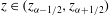
The multilayer approach considers a vertical partition of the domain in
 $N\in \mathbb{N}^{\ast }$
layers with preset thicknesses
$N\in \mathbb{N}^{\ast }$
layers with preset thicknesses
 $h_{{\it\alpha}}(t,x)$
for
$h_{{\it\alpha}}(t,x)$
for
 ${\it\alpha}=1,\ldots ,N$
, (see figure 1). Note that
${\it\alpha}=1,\ldots ,N$
, (see figure 1). Note that
 $\sum _{{\it\alpha}=1}^{N}h_{{\it\alpha}}=h$
. In practice, we set a vertical partition of the domain as follows: we introduce the positive coefficients
$\sum _{{\it\alpha}=1}^{N}h_{{\it\alpha}}=h$
. In practice, we set a vertical partition of the domain as follows: we introduce the positive coefficients
 $l_{{\it\alpha}}$
such that
$l_{{\it\alpha}}$
such that
 $$\begin{eqnarray}h_{{\it\alpha}}=l_{{\it\alpha}}h\quad \text{for }{\it\alpha}=1,\ldots ,N;\quad \mathop{\sum }_{{\it\alpha}=1}^{N}l_{{\it\alpha}}=1.\end{eqnarray}$$
Note that the thickness of each layer is automatically adapted to the movement of the free surface, since it depends on the total thickness of the mass flow. These layers are separated by
 $N+1$
interfaces
$N+1$
interfaces
 ${\it\Gamma}_{{\it\alpha}+1/2}(t)$
, which are described by the equations
${\it\Gamma}_{{\it\alpha}+1/2}(t)$
, which are described by the equations
 $z=z_{{\it\alpha}+1/2}(t,x)$
for
$z=z_{{\it\alpha}+1/2}(t,x)$
for
 ${\it\alpha}=0,1,\ldots ,N$
,
${\it\alpha}=0,1,\ldots ,N$
,
 $x\in I_{F}(t)$
. We assume that these interfaces are smooth enough. Observe that the fixed bottom and the free surface are respectively
$x\in I_{F}(t)$
. We assume that these interfaces are smooth enough. Observe that the fixed bottom and the free surface are respectively
 $b=z_{1/2}$
and
$b=z_{1/2}$
and
 $b+h=z_{N+1/2}$
, corresponding to the interfaces at the bottom
$b+h=z_{N+1/2}$
, corresponding to the interfaces at the bottom
 ${\it\Gamma}_{1/2}$
and at the free surface
${\it\Gamma}_{1/2}$
and at the free surface
 ${\it\Gamma}_{N+1/2}$
respectively. Note that
${\it\Gamma}_{N+1/2}$
respectively. Note that
 $z_{{\it\alpha}+1/2}=b+\sum _{{\it\beta}=1}^{{\it\alpha}}h_{{\it\beta}}$
and
$z_{{\it\alpha}+1/2}=b+\sum _{{\it\beta}=1}^{{\it\alpha}}h_{{\it\beta}}$
and
 $h_{{\it\alpha}}=z_{{\it\alpha}+1/2}-z_{{\it\alpha}-1/2}$
, for
$h_{{\it\alpha}}=z_{{\it\alpha}+1/2}-z_{{\it\alpha}-1/2}$
, for
 ${\it\alpha}=1,\ldots ,N$
. The subdomain between
${\it\alpha}=1,\ldots ,N$
. The subdomain between
 ${\it\Gamma}_{{\it\alpha}-1/2}$
and
${\it\Gamma}_{{\it\alpha}-1/2}$
and
 ${\it\Gamma}_{{\it\alpha}+1/2}$
is denoted by
${\it\Gamma}_{{\it\alpha}+1/2}$
is denoted by
 ${\it\Omega}_{{\it\alpha}}(t)$
, for a positive
${\it\Omega}_{{\it\alpha}}(t)$
, for a positive
 $t\in [0,T]$
,
$t\in [0,T]$
,
 $$\begin{eqnarray}{\it\Omega}_{{\it\alpha}}(t)=\{(x,z);x\in I_{F}(t)\text{ and }z_{{\it\alpha}-1/2}<z<z_{{\it\alpha}+1/2}\}.\end{eqnarray}$$
We need to introduce a specific notation about the approximations of the variables on the interfaces (see figure 1). For a function
 $f$
and for
$f$
and for
 ${\it\alpha}=0,1,\ldots ,N$
, we set
${\it\alpha}=0,1,\ldots ,N$
, we set
 $$\begin{eqnarray}f_{{\it\alpha}+1/2}^{-}:=(f_{|_{{\it\Omega}_{{\it\alpha}}(t)}})_{|_{{\it\Gamma}_{{\it\alpha}+1/2}(t)}}\quad \text{and}\quad f_{{\it\alpha}+1/2}^{+}:=(f_{|_{{\it\Omega}_{{\it\alpha}+1}(t)}})_{|_{{\it\Gamma}_{{\it\alpha}+1/2}(t)}}.\end{eqnarray}$$
Note that if the function
 $f$
is continuous,
$f$
is continuous,
 $$\begin{eqnarray}f_{{\it\alpha}+1/2}:=f_{|_{{\it\Gamma}_{{\it\alpha}+1/2}(t)}}=f_{{\it\alpha}+1/2}^{+}=f_{{\it\alpha}+1/2}^{-}.\end{eqnarray}$$
In addition, for a given time
 $t$
, we denote
$t$
, we denote
 $$\begin{eqnarray}\boldsymbol{n}_{T,{\it\alpha}+1/2}=\frac{(\partial _{t}z_{{\it\alpha}+1/2},\partial _{x}z_{{\it\alpha}+1/2},-1)^{\prime }}{\sqrt{1+(\partial _{x}z_{{\it\alpha}+1/2})^{2}+(\partial _{t}z_{{\it\alpha}+1/2})^{2}}}\quad \text{and}\quad \boldsymbol{n}_{{\it\alpha}+1/2}=\frac{(\partial _{x}z_{{\it\alpha}+1/2},-1)^{\prime }}{\sqrt{1+(\partial _{x}z_{{\it\alpha}+1/2})^{2}}},\end{eqnarray}$$
the space–time unit normal vector and the space unit normal vector to the interface
 ${\it\Gamma}_{{\it\alpha}+1/2}(t)$
outward to the layer
${\it\Gamma}_{{\it\alpha}+1/2}(t)$
outward to the layer
 ${\it\Omega}_{{\it\alpha}+1}(t)$
for
${\it\Omega}_{{\it\alpha}+1}(t)$
for
 ${\it\alpha}=0,\ldots ,N$
.
${\it\alpha}=0,\ldots ,N$
.
3.2.2 Weak solution with discontinuities
We are looking for a particular weak solution
 $(\boldsymbol{u},p,{\it\rho})$
of (3.11) (see Fernández-Nieto et al.
Reference Fernández-Nieto, Koné and Chacón Rebollo2014). We remind the reader that this solution must meet the following conditions:
$(\boldsymbol{u},p,{\it\rho})$
of (3.11) (see Fernández-Nieto et al.
Reference Fernández-Nieto, Koné and Chacón Rebollo2014). We remind the reader that this solution must meet the following conditions:
-
(i)
$(\boldsymbol{u},p,{\it\rho})$
is a standard weak solution of (3.11) in each layer
${\it\Omega}_{{\it\alpha}}(t)$
, -
(ii)
$(\boldsymbol{u},p,{\it\rho})$
satisfies the normal flux jump condition for mass and momentum at the interfaces
${\it\Gamma}_{{\it\alpha}+1/2}(t)$
, namely: (3.18)
$$\begin{eqnarray}\left.\begin{array}{@{}c@{}}[({\it\rho};{\it\rho}\boldsymbol{u})]_{{\it\alpha}+1/2}~\boldsymbol{n}_{T,{\it\alpha}+1/2}=0,\\ \displaystyle \left[\left({\it\rho}\boldsymbol{u};{\it\rho}\boldsymbol{u}\otimes \boldsymbol{u}-\frac{1}{{\it\varepsilon}}{\bf\sigma}\right)\right]_{{\it\alpha}+1/2}~\boldsymbol{n}_{T,{\it\alpha}+1/2}=0,\end{array}\right\}\end{eqnarray}$$


where
 $[(a;b)]_{{\it\alpha}+1/2}$
denotes the jump of
$[(a;b)]_{{\it\alpha}+1/2}$
denotes the jump of
 $(a;b)$
across the interface
$(a;b)$
across the interface
 ${\it\Gamma}_{{\it\alpha}+1/2}(t)$
.
${\it\Gamma}_{{\it\alpha}+1/2}(t)$
.
There are two main differences with the derivation in Fernández-Nieto et al. (Reference Fernández-Nieto, Koné and Chacón Rebollo2014): first, the
 ${\it\mu}(I)$
-rheology produces a non-constant viscosity coefficient, which implies an additional difficulty in order to develop the momentum balances at the interfaces. Second, the system to be solved is an asymptotic approximation of the Navier–Stokes equations, which helps to resolve the previous difficulty since we look for a first-order approximation in
${\it\mu}(I)$
-rheology produces a non-constant viscosity coefficient, which implies an additional difficulty in order to develop the momentum balances at the interfaces. Second, the system to be solved is an asymptotic approximation of the Navier–Stokes equations, which helps to resolve the previous difficulty since we look for a first-order approximation in
 ${\it\varepsilon}$
.
${\it\varepsilon}$
.
A particular family of velocity functions is considered, by assuming that the thickness of each layer is small enough to make the horizontal velocities independent of the vertical variable
 $z$
(usual shallow domain hypothesis). As a consequence, thanks to the incompressibility condition in each layer, we obtain that vertical velocities are linear in
$z$
(usual shallow domain hypothesis). As a consequence, thanks to the incompressibility condition in each layer, we obtain that vertical velocities are linear in
 $z$
and maybe discontinuous. We denote the velocity in each layer as
$z$
and maybe discontinuous. We denote the velocity in each layer as
 $$\begin{eqnarray}\boldsymbol{u}_{|_{{\it\Omega}_{{\it\alpha}}(t)}}:=\boldsymbol{u}_{{\it\alpha}}:=(u_{{\it\alpha}},w_{{\it\alpha}})^{\prime },\end{eqnarray}$$
where
 $u_{{\it\alpha}}$
and
$u_{{\it\alpha}}$
and
 $w_{{\it\alpha}}$
are the horizontal and vertical velocities, respectively, on layer
$w_{{\it\alpha}}$
are the horizontal and vertical velocities, respectively, on layer
 ${\it\alpha}$
. Then,
${\it\alpha}$
. Then,
 $$\begin{eqnarray}\partial _{z}u_{{\it\alpha}}=0;\quad \partial _{z}w_{{\it\alpha}}=d_{{\it\alpha}}(t,x)\end{eqnarray}$$
for some smooth function
 $d_{{\it\alpha}}(t,x)$
.
$d_{{\it\alpha}}(t,x)$
.
Pressure
From the asymptotic analysis, we directly get a hydrostatic pressure that is obtained from the vertical momentum equation in (3.4):
 $$\begin{eqnarray}\partial _{z}p_{{\it\alpha}}=-{\it\rho}\frac{1}{Fr^{2}}+O({\it\varepsilon}).\end{eqnarray}$$
By the continuity of the dynamic pressure, we can deduce at first order that
 $$\begin{eqnarray}p_{{\it\alpha}}(z)=\frac{{\it\rho}}{Fr^{2}}(b+h-z).\end{eqnarray}$$
Mass conservation across the interfaces and normal velocity
The mass conservation jump condition gives us the definition of the normal mass flux at the interface
 ${\it\Gamma}_{{\it\alpha}+1/2}(t)$
, denoted by
${\it\Gamma}_{{\it\alpha}+1/2}(t)$
, denoted by
 $G_{{\it\alpha}+1/2}:=G_{{\it\alpha}+1/2}^{+}=G_{{\it\alpha}+1/2}^{-}$
for:
$G_{{\it\alpha}+1/2}:=G_{{\it\alpha}+1/2}^{+}=G_{{\it\alpha}+1/2}^{-}$
for:
 $$\begin{eqnarray}G_{{\it\alpha}+1/2}^{\pm }=\partial _{t}z_{{\it\alpha}+1/2}+u_{{\it\alpha}+1/2}^{\pm }\,\partial _{x}z_{{\it\alpha}+1/2}-w_{{\it\alpha}+1/2}^{\pm }.\end{eqnarray}$$
By integrating the incompressibility equation and using this mass conservation condition, we get the definition of the vertical velocity
 $w_{{\it\alpha}}$
for
$w_{{\it\alpha}}$
for
 $\boldsymbol{u}_{{\it\alpha}}$
a solution of (3.11) (see Fernández-Nieto et al.
Reference Fernández-Nieto, Koné and Chacón Rebollo2014 for details). Thus, if we consider that there is no mass transference with the bottom (i.e.
$\boldsymbol{u}_{{\it\alpha}}$
a solution of (3.11) (see Fernández-Nieto et al.
Reference Fernández-Nieto, Koné and Chacón Rebollo2014 for details). Thus, if we consider that there is no mass transference with the bottom (i.e.
 $G_{1/2}=0$
), we obtain
$G_{1/2}=0$
), we obtain
 $$\begin{eqnarray}w_{1/2}^{+}=u_{1}\partial _{x}b+\partial _{t}b,\end{eqnarray}$$
and for
 ${\it\alpha}=1,\ldots ,N$
and
${\it\alpha}=1,\ldots ,N$
and
 $z\in (z_{{\it\alpha}-1/2},z_{{\it\alpha}+1/2})$
,
$z\in (z_{{\it\alpha}-1/2},z_{{\it\alpha}+1/2})$
,
 $$\begin{eqnarray}\left.\begin{array}{@{}c@{}}w_{{\it\alpha}}(t,x,z)=w_{{\it\alpha}-1/2}^{+}(t,x)-(z-z_{{\it\alpha}-1/2})\partial _{x}u_{{\it\alpha}}(t,x),\\ w_{{\it\alpha}+1/2}^{+}=(u_{{\it\alpha}+1}-u_{{\it\alpha}})\partial _{x}z_{{\it\alpha}+1/2}+w_{{\it\alpha}+1/2}^{-},\end{array}\right\}\end{eqnarray}$$
where
 $$\begin{eqnarray}w_{{\it\alpha}+1/2}^{-}=w_{{\it\alpha}-1/2}^{+}-h_{{\it\alpha}}\partial _{x}u_{{\it\alpha}}.\end{eqnarray}$$
Momentum conservation across the interfaces
The momentum jump conditions become:
 $$\begin{eqnarray}\frac{1}{{\it\varepsilon}}[{\bf\sigma}]_{{\it\alpha}+1/2}\boldsymbol{n}_{{\it\alpha}+1/2}=\frac{{\it\rho}\,G_{{\it\alpha}+1/2}}{\sqrt{1+|\partial _{x}z_{{\it\alpha}+1/2}|^{2}}}\,[\boldsymbol{u}]_{{\it\alpha}+1/2},\end{eqnarray}$$
where, for
 ${\it\alpha}=1,\ldots ,N-1$
, the total stress tensor is
${\it\alpha}=1,\ldots ,N-1$
, the total stress tensor is
 $$\begin{eqnarray}{\bf\sigma}_{{\it\alpha}+1/2}^{\pm }=-p_{{\it\alpha}+1/2}\mathscr{E}+{\bf\tau}_{{\it\varepsilon},{\it\alpha}+1/2}^{\pm },\end{eqnarray}$$
with
 $p_{{\it\alpha}+1/2}=p_{{\it\alpha}+1/2}^{+}=p_{{\it\alpha}+1/2}^{-}$
and
$p_{{\it\alpha}+1/2}=p_{{\it\alpha}+1/2}^{+}=p_{{\it\alpha}+1/2}^{-}$
and
 ${\bf\tau}_{{\it\varepsilon},{\it\alpha}+1/2}^{\pm }$
approximations of
${\bf\tau}_{{\it\varepsilon},{\it\alpha}+1/2}^{\pm }$
approximations of
 $p_{{\it\alpha}}$
and
$p_{{\it\alpha}}$
and
 ${\bf\tau}_{{\it\varepsilon},{\it\alpha}}$
at
${\bf\tau}_{{\it\varepsilon},{\it\alpha}}$
at
 ${\it\Gamma}_{{\it\alpha}+1/2}$
. Following Fernández-Nieto et al. (Reference Fernández-Nieto, Koné and Chacón Rebollo2014), we finally get that the momentum jump condition gives
${\it\Gamma}_{{\it\alpha}+1/2}$
. Following Fernández-Nieto et al. (Reference Fernández-Nieto, Koné and Chacón Rebollo2014), we finally get that the momentum jump condition gives
 $$\begin{eqnarray}{\bf\tau}_{{\it\varepsilon},{\it\alpha}+1/2}^{\pm }\boldsymbol{n}_{{\it\alpha}+1/2}=\widetilde{{\bf\tau}}_{{\it\varepsilon},{\it\alpha}+1/2}~\boldsymbol{n}_{{\it\alpha}+1/2}\pm \frac{1}{2}\frac{{\it\varepsilon}{\it\rho}G_{{\it\alpha}+1/2}}{\sqrt{1+|\partial _{x}z_{{\it\alpha}+1/2}|^{2}}}[\boldsymbol{u}]_{|_{{\it\Gamma}_{{\it\alpha}+1/2}(t)}},\end{eqnarray}$$
where
 $\widetilde{{\bf\tau}}_{{\it\varepsilon},{\it\alpha}+1/2}$
is an approximation of
$\widetilde{{\bf\tau}}_{{\it\varepsilon},{\it\alpha}+1/2}$
is an approximation of
 $({\it\eta}\unicode[STIX]{x1D63F}_{{\it\varepsilon}}(\boldsymbol{u}_{{\it\alpha}}))_{|{\it\Gamma}_{{\it\alpha}+1/2}}$
, defined by
$({\it\eta}\unicode[STIX]{x1D63F}_{{\it\varepsilon}}(\boldsymbol{u}_{{\it\alpha}}))_{|{\it\Gamma}_{{\it\alpha}+1/2}}$
, defined by
 $$\begin{eqnarray}\widetilde{{\bf\tau}}_{{\it\varepsilon},{\it\alpha}+1/2}={\it\eta}_{{\it\alpha}+1/2}\widetilde{\unicode[STIX]{x1D63F}}_{{\it\varepsilon},{\it\alpha}+1/2}=\frac{1}{2}{\it\eta}_{{\it\alpha}+1/2}\left(\begin{array}{@{}cc@{}}\displaystyle 2{\it\varepsilon}^{2}\partial _{x}\left(\frac{u_{{\it\alpha}+1/2}^{+}+u_{{\it\alpha}+1/2}^{-}}{2}\right) & \widetilde{\unicode[STIX]{x1D63F}}_{{\it\varepsilon},{\it\alpha}+1/2,xz}\\ \left(\widetilde{\unicode[STIX]{x1D63F}}_{{\it\varepsilon},{\it\alpha}+1/2,xz}\right)^{\prime } & 2{\mathscr{U}_{\mathscr{Z}}^{V}}_{,{\it\alpha}+1/2}\end{array}\right).\quad\end{eqnarray}$$
In this equation,
 $$\begin{eqnarray}\widetilde{\unicode[STIX]{x1D63F}}_{{\it\varepsilon},{\it\alpha}+1/2,xz}={\it\varepsilon}^{2}\partial _{x}\left(\frac{w_{{\it\alpha}+1/2}^{+}+w_{{\it\alpha}+1/2}^{-}}{2}\right)+{\mathscr{U}_{\mathscr{Z}}^{H}}_{,{\it\alpha}+1/2},\end{eqnarray}$$
and
 $({\mathscr{U}_{\mathscr{Z}}^{H}}_{,{\it\alpha}+1/2},{\mathscr{U}_{\mathscr{Z}}^{V}}_{,{\it\alpha}+1/2})$
is defined to approximate the derivatives in
$({\mathscr{U}_{\mathscr{Z}}^{H}}_{,{\it\alpha}+1/2},{\mathscr{U}_{\mathscr{Z}}^{V}}_{,{\it\alpha}+1/2})$
is defined to approximate the derivatives in
 $z$
. We remind the reader that we use a mixed formulation because of the possible vertical discontinuous profile. Thus, the auxiliary unknown
$z$
. We remind the reader that we use a mixed formulation because of the possible vertical discontinuous profile. Thus, the auxiliary unknown
 $\mathscr{U}_{\mathscr{Z}}$
satisfies
$\mathscr{U}_{\mathscr{Z}}$
satisfies
 $$\begin{eqnarray}\mathscr{U}_{\mathscr{Z}}-\partial _{z}\boldsymbol{u}=0,\quad \text{with}~\mathscr{U}_{\mathscr{Z}}=(\mathscr{U}_{\mathscr{Z}}^{H},\mathscr{U}_{\mathscr{ Z}}^{V}).\end{eqnarray}$$
And to approximate
 $\mathscr{U}_{\mathscr{Z}}$
, we approximate
$\mathscr{U}_{\mathscr{Z}}$
, we approximate
 $\boldsymbol{u}$
by
$\boldsymbol{u}$
by
 $\widetilde{\boldsymbol{u}}$
, a
$\widetilde{\boldsymbol{u}}$
, a
 $\mathbb{P}_{1}(z)$
interpolation such that
$\mathbb{P}_{1}(z)$
interpolation such that
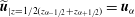 $\widetilde{\boldsymbol{u}}_{|z=1/2(z_{{\it\alpha}-1/2}+z_{{\it\alpha}+1/2})}=\boldsymbol{u}_{{\it\alpha}}$
. Then
$\widetilde{\boldsymbol{u}}_{|z=1/2(z_{{\it\alpha}-1/2}+z_{{\it\alpha}+1/2})}=\boldsymbol{u}_{{\it\alpha}}$
. Then
 ${\mathscr{U}_{\mathscr{Z}}}_{{\it\alpha}+1/2}=({\mathscr{U}_{\mathscr{Z}}^{H}}_{,{\it\alpha}+1/2},{\mathscr{U}_{\mathscr{Z}}^{V}}_{,{\it\alpha}+1/2})$
is an approximation of
${\mathscr{U}_{\mathscr{Z}}}_{{\it\alpha}+1/2}=({\mathscr{U}_{\mathscr{Z}}^{H}}_{,{\it\alpha}+1/2},{\mathscr{U}_{\mathscr{Z}}^{V}}_{,{\it\alpha}+1/2})$
is an approximation of
 $\mathscr{U}_{\mathscr{Z}}(\widetilde{\boldsymbol{u}})$
at
$\mathscr{U}_{\mathscr{Z}}(\widetilde{\boldsymbol{u}})$
at
 ${\it\Gamma}_{{\it\alpha}+1/2}$
.
${\it\Gamma}_{{\it\alpha}+1/2}$
.
Let us remark that the previous expression of the tensor
 $\widetilde{{\bf\tau}}_{{\it\varepsilon},{\it\alpha}+1/2}$
in (3.30) has the same structure as the original case in Fernández-Nieto et al. (Reference Fernández-Nieto, Koné and Chacón Rebollo2014), except for the viscosity that now is not constant because it is defined by the
$\widetilde{{\bf\tau}}_{{\it\varepsilon},{\it\alpha}+1/2}$
in (3.30) has the same structure as the original case in Fernández-Nieto et al. (Reference Fernández-Nieto, Koné and Chacón Rebollo2014), except for the viscosity that now is not constant because it is defined by the
 ${\it\mu}(I)$
-rheology in (2.11). Then, we must give an approximation of the viscosity at the interface up to first order in
${\it\mu}(I)$
-rheology in (2.11). Then, we must give an approximation of the viscosity at the interface up to first order in
 ${\it\varepsilon}$
, which we denoted by
${\it\varepsilon}$
, which we denoted by
 ${\it\eta}_{{\it\alpha}+1/2}$
. We have considered the following first-order approximation of
${\it\eta}_{{\it\alpha}+1/2}$
. We have considered the following first-order approximation of
 $\Vert \unicode[STIX]{x1D63F}(\boldsymbol{u})\Vert$
at
$\Vert \unicode[STIX]{x1D63F}(\boldsymbol{u})\Vert$
at
 $z=z_{{\it\alpha}+1/2}$
,
$z=z_{{\it\alpha}+1/2}$
,
 $$\begin{eqnarray}\Vert \unicode[STIX]{x1D63F}(\boldsymbol{u})\Vert _{{\it\alpha}+1/2}\approx |{\mathscr{U}_{\mathscr{Z}}^{H}}_{,{\it\alpha}+1/2}|.\end{eqnarray}$$
Then, it reads
 $$\begin{eqnarray}{\it\eta}_{{\it\alpha}+1/2}={\it\eta}_{{\it\alpha}+1/2}({\mathscr{U}_{\mathscr{Z}}^{H}}_{,{\it\alpha}+1/2})=\frac{{\it\mu}(I_{{\it\alpha}+1/2})p_{{\it\alpha}+1/2}}{\max \left(|{\mathscr{U}_{\mathscr{Z}}^{H}}_{,{\it\alpha}+1/2}|,\displaystyle \frac{{\it\mu}(I_{{\it\alpha}+1/2})p_{{\it\alpha}+1/2}}{{\it\eta}_{M}}\right)},\end{eqnarray}$$
with
 $$\begin{eqnarray}{\mathscr{U}_{\mathscr{Z}}^{H}}_{,{\it\alpha}+1/2}=\frac{u_{{\it\alpha}+1}-u_{{\it\alpha}}}{h_{{\it\alpha}+1/2}},\quad \text{for}~{\it\alpha}=1,\ldots ,N-1,\end{eqnarray}$$
with
 $h_{{\it\alpha}+1/2}$
being the distance between the midpoints of layers
$h_{{\it\alpha}+1/2}$
being the distance between the midpoints of layers
 ${\it\alpha}$
and
${\it\alpha}$
and
 ${\it\alpha}+1$
. Moreover,
${\it\alpha}+1$
. Moreover,
 $$\begin{eqnarray}{\mathscr{U}_{\mathscr{Z}}^{H}}_{,1/2}=\frac{u_{1}}{h_{1}},\end{eqnarray}$$
and
 $$\begin{eqnarray}p_{{\it\alpha}+1/2}=\frac{{\it\rho}}{Fr^{2}}\mathop{\sum }_{{\it\beta}={\it\alpha}+1}^{N}h_{{\it\beta}},\quad I_{{\it\alpha}+1/2}=\frac{2\,d_{s}|{\mathscr{U}_{\mathscr{Z}}^{H}}_{,{\it\alpha}+1/2}|}{\sqrt{p_{{\it\alpha}+1/2}/{\it\rho}_{s}}},\quad \text{for}~{\it\alpha}=0,\ldots ,N-1.\end{eqnarray}$$
Note that
 ${\it\eta}_{N+1/2}=0$
, because we suppose that the atmospheric pressure is zero.
${\it\eta}_{N+1/2}=0$
, because we suppose that the atmospheric pressure is zero.
3.3 Final model
The final model is derived as in Fernández-Nieto et al. (Reference Fernández-Nieto, Koné and Chacón Rebollo2014) by looking for a particular weak solution of the asymptotic system (3.11). First (3.11) are multiplied by some test functions, and secondly we integrate this system in the domain
 ${\it\Omega}_{{\it\alpha}}(t)$
(see appendix A for more details). In this way, the final
${\it\Omega}_{{\it\alpha}}(t)$
(see appendix A for more details). In this way, the final
 ${\it\mu}(I)$
-rheology multilayer model is obtained in dimensionless variables. The last step is to come back to the original variables taking into account the assumptions described in § 3.1. As a result, the final model reads, for
${\it\mu}(I)$
-rheology multilayer model is obtained in dimensionless variables. The last step is to come back to the original variables taking into account the assumptions described in § 3.1. As a result, the final model reads, for
 ${\it\alpha}=1,\ldots ,N$
,
${\it\alpha}=1,\ldots ,N$
,
 $$\begin{eqnarray}\displaystyle \left.\begin{array}{@{}l@{}}l_{{\it\alpha}}(\partial _{t}h+\partial _{x}(hu_{{\it\alpha}}))=G_{{\it\alpha}+1/2}-G_{{\it\alpha}-1/2},\\ l_{{\it\alpha}}({\it\rho}\partial _{t}(hu_{{\it\alpha}})+{\it\rho}\partial _{x}(hu_{{\it\alpha}}^{2})+{\it\rho}g\cos {\it\theta}h\partial _{x}(b+\tilde{b}+h))\\ \quad =K_{{\it\alpha}-1/2}-K_{{\it\alpha}+1/2}+{\textstyle \frac{1}{2}}{\it\rho}G_{{\it\alpha}+1/2}(u_{{\it\alpha}+1}+u_{{\it\alpha}})-{\textstyle \frac{1}{2}}{\it\rho}G_{{\it\alpha}-1/2}(u_{{\it\alpha}}+u_{{\it\alpha}-1}),\end{array}\right\} & & \displaystyle\end{eqnarray}$$
where
 $G_{{\it\alpha}+1/2}$
are given in (3.23),
$G_{{\it\alpha}+1/2}$
are given in (3.23),
 $$\begin{eqnarray}K_{{\it\alpha}+1/2}=-{\it\eta}_{{\it\alpha}+1/2}({\mathscr{U}_{\mathscr{Z}}^{H}}_{,{\it\alpha}+1/2}){\mathscr{U}_{\mathscr{Z}}^{H}}_{,{\it\alpha}+1/2}\quad \text{and}\quad K_{1/2}=-{\it\mu}(I_{1/2}){\it\rho}g\cos {\it\theta}\,h\frac{u_{1}}{|u_{1}|},\end{eqnarray}$$
for
 ${\it\eta}_{{\it\alpha}+1/2}$
defined in (3.34)–(3.37).
${\it\eta}_{{\it\alpha}+1/2}$
defined in (3.34)–(3.37).
Note that the proposed model (3.38) has
 $2N$
equations and unknowns:
$2N$
equations and unknowns:
 $(h,\{hu_{{\it\alpha}}\}_{{\it\alpha}=1,\ldots ,N},\{G_{{\it\alpha}+1/2}\}_{{\it\alpha}=1,\ldots ,N-1})$
. But thanks to (3.23)–(3.25) we can write
$(h,\{hu_{{\it\alpha}}\}_{{\it\alpha}=1,\ldots ,N},\{G_{{\it\alpha}+1/2}\}_{{\it\alpha}=1,\ldots ,N-1})$
. But thanks to (3.23)–(3.25) we can write
 $$\begin{eqnarray}G_{{\it\alpha}+1/2}=\partial _{t}z_{{\it\alpha}+1/2}+\frac{u_{{\it\alpha}}+u_{{\it\alpha}+1}}{2}\partial _{x}z_{{\it\alpha}+1/2}-w_{{\it\alpha}+1/2},\quad \text{where}~w_{{\it\alpha}+1/2}=\frac{w_{{\it\alpha}+1/2}^{+}+w_{{\it\alpha}+1/2}^{-}}{2}.\end{eqnarray}$$
As a consequence, the system has
 $2N$
unknowns that are also the total height (
$2N$
unknowns that are also the total height (
 $h$
), the discharge at each layer (
$h$
), the discharge at each layer (
 $\{hu_{{\it\alpha}}\}_{{\it\alpha}=1,\ldots ,N}$
) and the averaged vertical velocity at each internal interface (
$\{hu_{{\it\alpha}}\}_{{\it\alpha}=1,\ldots ,N}$
) and the averaged vertical velocity at each internal interface (
 $\{w_{{\it\alpha}+1/2}\}_{{\it\alpha}=1,\ldots ,N-1}$
).
$\{w_{{\it\alpha}+1/2}\}_{{\it\alpha}=1,\ldots ,N-1}$
).
Nevertheless, by combining the continuity equations, the system can be rewritten with
 $N+1$
equations and unknowns. The unknowns of the reduced system are the total height
$N+1$
equations and unknowns. The unknowns of the reduced system are the total height
 $(h)$
and the discharge of each layer,
$(h)$
and the discharge of each layer,
 $$\begin{eqnarray}q_{{\it\alpha}}=h\,u_{{\it\alpha}},\quad \text{for }{\it\alpha}=1,\ldots ,N.\end{eqnarray}$$
By introducing (see Fernández-Nieto et al. Reference Fernández-Nieto, Koné and Chacón Rebollo2014)
 $$\begin{eqnarray}\displaystyle {\it\xi}_{{\it\alpha},{\it\gamma}}=\left\{\begin{array}{@{}ll@{}}(1-(l_{1}+\cdots +l_{{\it\alpha}}))l_{{\it\gamma}},\quad & \text{if }{\it\gamma}\leqslant {\it\alpha},\\ -(l_{1}+\cdots +l_{{\it\alpha}})l_{{\it\gamma}},\quad & \text{otherwise},\end{array}\right. & & \displaystyle\end{eqnarray}$$
for
 ${\it\alpha},{\it\gamma}\in \{1,\ldots ,N\}$
, the system (3.38)–(3.39) is rewritten as
${\it\alpha},{\it\gamma}\in \{1,\ldots ,N\}$
, the system (3.38)–(3.39) is rewritten as
 $$\begin{eqnarray}\left.\begin{array}{@{}l@{}}\displaystyle \partial _{t}h+\partial _{x}\left(\mathop{\sum }_{{\it\beta}=1}^{N}l_{{\it\beta}}q_{{\it\beta}}\right)=0,\\ \displaystyle \partial _{t}q_{{\it\alpha}}+\partial _{x}\left(\frac{q_{{\it\alpha}}^{2}}{h}+g\cos {\it\theta}\frac{h^{2}}{2}\right)+g\cos {\it\theta}\,h\,\partial _{x}z_{b}\\ \displaystyle \qquad +\,\mathop{\sum }_{{\it\gamma}=1}^{N}\frac{1}{2hl_{{\it\alpha}}}((q_{{\it\alpha}}+q_{{\it\alpha}-1}){\it\xi}_{{\it\alpha}-1,{\it\gamma}}-(q_{{\it\alpha}+1}+q_{{\it\alpha}}){\it\xi}_{{\it\alpha},{\it\gamma}})\partial _{x}q_{{\it\gamma}}\\ \displaystyle \quad =\frac{1}{{\it\rho}l_{{\it\alpha}}}(\boldsymbol{K}_{{\it\alpha}-1/2}-\boldsymbol{K}_{{\it\alpha}+1/2})\quad {\it\alpha}=1,\ldots ,N,\end{array}\right\}\end{eqnarray}$$
where
 $z_{b}=b+\tilde{b}$
has been introduced for simplicity.
$z_{b}=b+\tilde{b}$
has been introduced for simplicity.
Moreover, we can see that this model satisfies a dissipative energy inequality. Denoting the energy of the layer
 ${\it\alpha}=1,\ldots ,N$
for the system (3.38)–(3.39) by
${\it\alpha}=1,\ldots ,N$
for the system (3.38)–(3.39) by
 $$\begin{eqnarray}E_{{\it\alpha}}=h_{{\it\alpha}}\left(\frac{|u_{{\it\alpha}}|^{2}}{2}+g\cos {\it\theta}\left(z_{b}+\frac{h}{2}\right)\right),\end{eqnarray}$$
the following dissipative energy inequality is satisfied:
 $$\begin{eqnarray}\displaystyle & & \displaystyle {\it\rho}\partial _{t}\left(\mathop{\sum }_{{\it\alpha}=1}^{N}E_{{\it\alpha}}\right)+{\it\rho}\partial _{x}\left[\mathop{\sum }_{{\it\alpha}=1}^{N}u_{{\it\alpha}}\left(E_{{\it\alpha}}+{\it\rho}g\cos {\it\theta}\,h_{{\it\alpha}}\frac{h}{2}\right)\right]\nonumber\\ \displaystyle & & \displaystyle \quad \leqslant -{\it\rho}g\cos {\it\theta}\,h|u_{1}|{\it\mu}(I)-\frac{|u_{N}|^{2}}{h_{N}}{\it\eta}_{N+1/2}-\mathop{\sum }_{{\it\alpha}=1}^{N-1}\frac{(u_{{\it\alpha}+1}-u_{{\it\alpha}})^{2}}{h_{{\it\alpha}+1/2}}{\it\eta}_{{\it\alpha}+1/2}.\end{eqnarray}$$
Finally, note that if we consider a no-slip condition to deduce the model instead of the Coulomb friction condition (2.16), the only difference that appears in the multilayer approach is the definition of
 $K_{1/2}$
. It must be defined directly in terms of the rheology, in the same way as
$K_{1/2}$
. It must be defined directly in terms of the rheology, in the same way as
 $K_{{\it\alpha}+1/2}$
for
$K_{{\it\alpha}+1/2}$
for
 ${\it\alpha}=1,\ldots ,N-1$
. That is,
${\it\alpha}=1,\ldots ,N-1$
. That is,
 $$\begin{eqnarray}K_{1/2}=-{\it\eta}_{1/2}({\mathscr{U}_{\mathscr{Z}}^{H}}_{,1/2})\,{\mathscr{U}_{\mathscr{Z}}^{H}}_{,1/2},\end{eqnarray}$$
where
 ${\mathscr{U}_{\mathscr{Z}}^{H}}_{,1/2}$
is an approximation of the horizontal component of the solution of (3.32) for
${\mathscr{U}_{\mathscr{Z}}^{H}}_{,1/2}$
is an approximation of the horizontal component of the solution of (3.32) for
 $z=b$
. Then, using the no-slip condition, a second-order approximation is
$z=b$
. Then, using the no-slip condition, a second-order approximation is
 $$\begin{eqnarray}{\mathscr{U}_{\mathscr{Z}}^{H}}_{,1/2}=\frac{2\,u_{1}}{h_{1}}.\end{eqnarray}$$
4 Numerical tests
The numerical approximation is performed in 2D (downslope and normal directions). We rewrite the model as a non-conservative hyperbolic system with source terms as in Fernández-Nieto et al. (Reference Fernández-Nieto, Koné and Chacón Rebollo2014). Then a splitting procedure is considered.
First, we set aside the term that appears in the internal interfaces and a standard path-conservative finite volume method is applied. These path-conservative methods were introduced in Parés (Reference Parés2006). To deal with the Coulomb friction term, we use the hydrostatic reconstruction introduced in Audusse et al. (Reference Audusse, Bouchut, Bristeau, Klein and Perthame2004), which is applied in Bouchut (Reference Bouchut2004) to solve the Saint-Venant system with Coulomb friction. The main advantage of this reconstruction is its great stability.
The second step is to solve the contribution of the term in the internal interfaces, which represents the mass and momentum exchange between layers. In this step, a semi-implicit scheme is employed, taking into account the regularization of
 $\Vert \unicode[STIX]{x1D63F}(\boldsymbol{u}_{{\it\alpha}})\Vert$
mentioned in § 2.2 in order to avoid the singularity when
$\Vert \unicode[STIX]{x1D63F}(\boldsymbol{u}_{{\it\alpha}})\Vert$
mentioned in § 2.2 in order to avoid the singularity when
 $\Vert \unicode[STIX]{x1D63F}(\boldsymbol{u}_{{\it\alpha}})\Vert$
vanishes.
$\Vert \unicode[STIX]{x1D63F}(\boldsymbol{u}_{{\it\alpha}})\Vert$
vanishes.
In order to validate the multilayer shallow model (denoted MSM hereafter) with the
 ${\it\mu}(I)$
-rheology, we compare it to (i) 2D steady and transient uniform flows over inclined surfaces with and without the effect of sidewall friction (analytical solutions and experimental data for deep and surface flows), (ii) laboratory experiments of highly transient and non-uniform granular flows over inclined planes covered by an erodible bed, in which case the shape of the velocity profiles strongly changes with time and space.
${\it\mu}(I)$
-rheology, we compare it to (i) 2D steady and transient uniform flows over inclined surfaces with and without the effect of sidewall friction (analytical solutions and experimental data for deep and surface flows), (ii) laboratory experiments of highly transient and non-uniform granular flows over inclined planes covered by an erodible bed, in which case the shape of the velocity profiles strongly changes with time and space.
4.1 Granular surface flows in a channel
In this subsection we deal with several Bagnold flows. First, we consider a uniform Bagnold flow without taking into account the effect of the lateral wall friction. Then, we show that our multilayer model is able to capture the velocity profiles for flows in a narrow channel when sidewall friction is introduced. In that case we compare with the analytical solution and laboratory experiments. Note that Bagnold flows verify, at the free surface
 $$\begin{eqnarray}p_{|z=H}=0\quad \text{and}\quad \Vert \unicode[STIX]{x1D63F}(u)\Vert _{|z=H}=|\partial _{z}u|_{|z=H}=0.\end{eqnarray}$$
Therefore, we cannot use the regularization (2.11) since its denominator vanishes at the free surface. In this case we use the regularization
 $$\begin{eqnarray}{\it\eta}=\frac{{\it\mu}(I)p}{\sqrt{\Vert \unicode[STIX]{x1D63F}(\boldsymbol{u})\Vert ^{2}+{\it\delta}^{2}}},\end{eqnarray}$$
where
 ${\it\delta}>0$
is a small parameter (see Bercovier & Engelman Reference Bercovier and Engelman1980).
${\it\delta}>0$
is a small parameter (see Bercovier & Engelman Reference Bercovier and Engelman1980).
4.1.1 Steady uniform Bagnold flow: analytical solution
Let us first compare the model with the analytical solution for a uniform flow over an inclined plane of slope
 ${\it\theta}$
and thickness
${\it\theta}$
and thickness
 $H>0$
, i.e. a Bagnold flow (see Silbert et al.
Reference Silbert, Ertaş, Grest, Halsey, Levine and Plimpton2001, GDR MiDi 2004 or Lagrée et al.
Reference Lagrée, Staron and Popinet2011). This solution is obtained by imposing zero pressure and zero shear stress at the free surface and a no-slip condition at the bottom (Coulomb friction can be easily changed by no-slip condition in the
$H>0$
, i.e. a Bagnold flow (see Silbert et al.
Reference Silbert, Ertaş, Grest, Halsey, Levine and Plimpton2001, GDR MiDi 2004 or Lagrée et al.
Reference Lagrée, Staron and Popinet2011). This solution is obtained by imposing zero pressure and zero shear stress at the free surface and a no-slip condition at the bottom (Coulomb friction can be easily changed by no-slip condition in the
 ${\it\mu}(I)$
-rheology multilayer model, see §§ 2.3 and 3.3).
${\it\mu}(I)$
-rheology multilayer model, see §§ 2.3 and 3.3).

Figure 2. Sketch of the analytical solution.
By denoting
 $u$
and
$u$
and
 $w$
the downslope and normal velocities,
$w$
the downslope and normal velocities,
 $p$
the pressure and
$p$
the pressure and
 ${\it\tau}$
the shear stress and by taking the rheological parameters defined in § 2.2, the steady uniform Bagnold flow is described by
${\it\tau}$
the shear stress and by taking the rheological parameters defined in § 2.2, the steady uniform Bagnold flow is described by
 $$\begin{eqnarray}\left.\begin{array}{@{}c@{}}\displaystyle u(z)=\frac{2}{3d_{s}}I_{0}\left(\frac{\tan {\it\theta}-{\it\mu}_{s}}{{\it\mu}_{2}-\tan {\it\theta}}\right)\sqrt{{\it\varphi}_{s}g\cos {\it\theta}}(H^{3/2}-(H-z)^{3/2}),\\ u(z=0)=0,\quad w=0,\\ p(z)={\it\rho}g\cos {\it\theta}(H-z),\\ {\it\tau}(z)={\it\mu}(I)p={\it\rho}g\sin {\it\theta}(H-z),\\ p(z=H)=0,\quad {\it\tau}(z=H)=0,\\ {\it\mu}(I)=\tan ({\it\theta}),\quad \text{for }z\in (0,H).\end{array}\right\}\end{eqnarray}$$
For the numerical simulation, as in the analytical solution, we consider a uniform flow with constant thickness
 $H=1$
m and velocity
$H=1$
m and velocity
 $u=w=0~\text{m}~\text{s}^{-1}$
at the initial time
$u=w=0~\text{m}~\text{s}^{-1}$
at the initial time
 $t=0$
s. The boundary conditions at the free surface and at the bottom have been set as in (4.3). At the right and left boundaries, we use open boundary conditions.
$t=0$
s. The boundary conditions at the free surface and at the bottom have been set as in (4.3). At the right and left boundaries, we use open boundary conditions.

Figure 3. Comparison between the analytical solution (dashed and solid lines) and the simulations obtained using the MSM with the
 ${\it\mu}(I)$
-rheology (symbols). (a) Analytical and simulated downslope horizontal velocity
${\it\mu}(I)$
-rheology (symbols). (a) Analytical and simulated downslope horizontal velocity
 $u$
, pressure
$u$
, pressure
 $p$
and strain rate
$p$
and strain rate
 $\Vert \unicode[STIX]{x1D63F}(\boldsymbol{u})\Vert$
. (b) Analytical and simulated shear stress and friction coefficient
$\Vert \unicode[STIX]{x1D63F}(\boldsymbol{u})\Vert$
. (b) Analytical and simulated shear stress and friction coefficient
 ${\it\mu}(I)$
. (c) Comparison between the simulated (symbols) and the exact (dashed line) horizontal velocity at the free surface as a function of the slope angle.
${\it\mu}(I)$
. (c) Comparison between the simulated (symbols) and the exact (dashed line) horizontal velocity at the free surface as a function of the slope angle.

Figure 4. (a) Computing time as a function of the number of layers in the MSM and (b) relative error between the computed and exact velocity for simulations over a slope of
 ${\it\theta}=24.64^{\circ }$
.
${\it\theta}=24.64^{\circ }$
.
We choose the rheological parameters
 $I_{0}=0.279$
and
$I_{0}=0.279$
and
 ${\it\mu}_{s}=0.38\approx \tan (20.8^{\circ })$
,
${\it\mu}_{s}=0.38\approx \tan (20.8^{\circ })$
,
 ${\it\mu}_{2}=0.62\approx \tan (31.8^{\circ })$
and the particle diameter
${\it\mu}_{2}=0.62\approx \tan (31.8^{\circ })$
and the particle diameter
 $d_{s}=4$
cm with solid volume fraction
$d_{s}=4$
cm with solid volume fraction
 ${\it\varphi}_{s}=0.62$
. The slope angle is taken as
${\it\varphi}_{s}=0.62$
. The slope angle is taken as
 ${\it\theta}=0.43~\text{rad}\approx 24.64^{\circ }$
. Figure 3 shows the good agreement between the simulated and exact solutions for the profiles of the velocity, pressure, shear stress,
${\it\theta}=0.43~\text{rad}\approx 24.64^{\circ }$
. Figure 3 shows the good agreement between the simulated and exact solutions for the profiles of the velocity, pressure, shear stress,
 ${\it\mu}(I)$
and
${\it\mu}(I)$
and
 $\Vert \unicode[STIX]{x1D63F}(u)\Vert$
. It also shows the downslope velocity at the free surface as a function of the slope angle. Note that for slopes smaller than
$\Vert \unicode[STIX]{x1D63F}(u)\Vert$
. It also shows the downslope velocity at the free surface as a function of the slope angle. Note that for slopes smaller than
 $\arctan ({\it\mu}_{s})$
, the surface velocity is close to zero (it is not equal to zero, because of the regularization method), namely
$\arctan ({\it\mu}_{s})$
, the surface velocity is close to zero (it is not equal to zero, because of the regularization method), namely
 $u(z=H)\sim 10^{-5}$
, so that the mass is almost at rest.
$u(z=H)\sim 10^{-5}$
, so that the mass is almost at rest.
These results are computed using 50 layers in the MSM. Note that we use a slope in the well-posed region described in Barker et al. (Reference Barker, Schaeffer, Bohorquez and Gray2015) for the full
 ${\it\mu}(I)$
-rheology, which is smaller than the well-posed region for the depth-averaged
${\it\mu}(I)$
-rheology, which is smaller than the well-posed region for the depth-averaged
 ${\it\mu}(I)$
-rheology (well-posed for
${\it\mu}(I)$
-rheology (well-posed for
 ${\it\delta}_{s}=20.8^{\circ }\leqslant {\it\theta}<{\it\delta}_{2}=31.8^{\circ }$
in the case of depth-averaged
${\it\delta}_{s}=20.8^{\circ }\leqslant {\it\theta}<{\it\delta}_{2}=31.8^{\circ }$
in the case of depth-averaged
 ${\it\mu}(I)$
-rheology). If we use a slope close enough to
${\it\mu}(I)$
-rheology). If we use a slope close enough to
 ${\it\delta}_{2}$
the system becomes unstable because of the ill-posedness of the full
${\it\delta}_{2}$
the system becomes unstable because of the ill-posedness of the full
 ${\it\mu}(I)$
-rheology in this region.
${\it\mu}(I)$
-rheology in this region.
Figure 4 shows the computing time required to simulate 50 seconds (on a laptop with Intel
 $^{\unicode[STIX]{x00AE} }$
Core™ i7-4500U and 8 GB of RAM) and the relative error between the computed velocity and the exact solution using a different number of layers and 30 nodes in the
$^{\unicode[STIX]{x00AE} }$
Core™ i7-4500U and 8 GB of RAM) and the relative error between the computed velocity and the exact solution using a different number of layers and 30 nodes in the
 $x$
-direction. In table 1 we show that second-order accuracy is reached in norms
$x$
-direction. In table 1 we show that second-order accuracy is reached in norms
 $L^{1}$
and
$L^{1}$
and
 $L^{2}$
, while in norm
$L^{2}$
, while in norm
 $L^{\infty }$
the order is over 1.5. This behaviour in norm
$L^{\infty }$
the order is over 1.5. This behaviour in norm
 $L^{\infty }$
is due to the boundary conditions at the free surface, where the analytical solution verifies that
$L^{\infty }$
is due to the boundary conditions at the free surface, where the analytical solution verifies that
 $\partial _{z}u=0$
.
$\partial _{z}u=0$
.
Table 1. Order of the error for the velocity of the Bagnold flow.

4.1.2 2D steady uniform flow in a channel: sidewalls effect on the velocity profile
The relevance of the lateral wall friction when a granular material flows in a channel has been proved by Jop et al. (Reference Jop, Forterre and Pouliquen2005) (see also Baker, Barker & Gray Reference Baker, Barker and Gray2016). Under the hypothesis of a steady uniform flow and neglecting the variations in the transverse direction, they propose to model this effect with a modified
 ${\it\mu}(I)$
-rheology by adding an extra term, which defines an effective friction term
${\it\mu}(I)$
-rheology by adding an extra term, which defines an effective friction term
 $$\begin{eqnarray}{\it\mu}(I)={\it\mu}_{s}+\frac{{\it\mu}_{2}-{\it\mu}_{s}}{I_{0}+I}I+{\it\mu}_{w}\frac{H-z}{W},\end{eqnarray}$$
where
 $W$
is the channel width,
$W$
is the channel width,
 ${\it\mu}_{w}$
is the constant coefficient of friction with the side walls and
${\it\mu}_{w}$
is the constant coefficient of friction with the side walls and
 $H$
the thickness of the flow. Note that this extra term (last term) increases when we get closer to the bottom from the free surface. In addition, for a channel slope
$H$
the thickness of the flow. Note that this extra term (last term) increases when we get closer to the bottom from the free surface. In addition, for a channel slope
 ${\it\theta}$
with respect to the horizontal axis, the analytical expression for the velocity profile reads (see appendix B in Jop et al.
Reference Jop, Forterre and Pouliquen2005):
${\it\theta}$
with respect to the horizontal axis, the analytical expression for the velocity profile reads (see appendix B in Jop et al.
Reference Jop, Forterre and Pouliquen2005):
 $$\begin{eqnarray}\displaystyle u(z) & = & \displaystyle 2\,\frac{I_{0}\sqrt{{\it\varphi}_{s}\,g\cos {\it\theta}}}{d_{s}}\left[\frac{1}{3}(H-z)^{3/2}-\frac{1}{3}(H-h^{\ast })^{3/2}\right.\nonumber\\ \displaystyle & & \displaystyle -\,\frac{{\it\mu}_{2}-{\it\mu}_{s}}{{\it\mu}_{w}}W((H-z)^{1/2}-(H-h^{\ast })^{1/2})\nonumber\\ \displaystyle & & \displaystyle \left.+\,\sqrt{h_{2}}\frac{{\it\mu}_{2}-{\it\mu}_{s}}{{\it\mu}_{w}}W\left(\arctan \sqrt{\frac{H-z}{h_{2}}}-\arctan \sqrt{\frac{H-h^{\ast }}{h_{2}}}\right)\right],\end{eqnarray}$$
where
 $$\begin{eqnarray}h^{\ast }=H-\frac{\tan {\it\theta}-{\it\mu}_{s}}{{\it\mu}_{w}}\,W,\quad h_{2}=\frac{{\it\mu}_{2}-\tan {\it\theta}}{{\it\mu}_{w}}\,W.\end{eqnarray}$$
Note that we can integrate the last equation and the discharge is obtained as a function of the slope
 ${\it\theta}$
. In these experiments, Jop et al. (Reference Jop, Forterre and Pouliquen2005) fixed the discharge and computed the velocity profile for different widths. We choose the same material and rheological properties and perform these experiments. The grain diameter is
${\it\theta}$
. In these experiments, Jop et al. (Reference Jop, Forterre and Pouliquen2005) fixed the discharge and computed the velocity profile for different widths. We choose the same material and rheological properties and perform these experiments. The grain diameter is
 $d_{s}=0.53$
mm and the volume fraction is
$d_{s}=0.53$
mm and the volume fraction is
 ${\it\varphi}_{s}=0.6$
. The rheological parameters are
${\it\varphi}_{s}=0.6$
. The rheological parameters are
 ${\it\mu}_{s}=\tan (20.9^{\circ })$
,
${\it\mu}_{s}=\tan (20.9^{\circ })$
,
 ${\it\mu}_{2}=\tan (32.76^{\circ })$
and
${\it\mu}_{2}=\tan (32.76^{\circ })$
and
 $I_{0}=0.279$
. The friction coefficient with the sidewalls is
$I_{0}=0.279$
. The friction coefficient with the sidewalls is
 ${\it\mu}_{w}=\tan (10.4^{\circ })$
. We set the thickness of the flow
${\it\mu}_{w}=\tan (10.4^{\circ })$
. We set the thickness of the flow
 $H=45d_{s}$
, the dimensionless discharge
$H=45d_{s}$
, the dimensionless discharge
 $Q^{\ast }=31.5$
and different widths of the channel are considered (
$Q^{\ast }=31.5$
and different widths of the channel are considered (
 $W=19d_{s}$
,
$W=19d_{s}$
,
 $57d_{s}$
,
$57d_{s}$
,
 $283d_{s}$
).
$283d_{s}$
).
Figure 5 shows the exact agreement between the analytical solution and the simulations for the velocity profile. In this case we consider 50 layers to obtain the solution. In table 2 we present the errors and accuracy order of the method for
 $W=283d_{s}$
. We obtain similar results to those presented in the previous subsection.
$W=283d_{s}$
. We obtain similar results to those presented in the previous subsection.

Figure 5. Comparison between the analytical solution (solid lines) and the simulations obtained using the MSM with the
 ${\it\mu}(I)$
-rheology (symbols) for the velocity profile for
${\it\mu}(I)$
-rheology (symbols) for the velocity profile for
 $Q^{\ast }=31.5$
, and different widths:
$Q^{\ast }=31.5$
, and different widths:
 $W=19d_{s}$
,
$W=19d_{s}$
,
 $W=57d_{s}$
and
$W=57d_{s}$
and
 $W=283d_{s}$
.
$W=283d_{s}$
.
Table 2. Order of the error for the velocity of the Bagnold flow with lateral wall effect. Case
 $W=283d_{s}$
.
$W=283d_{s}$
.

4.1.3 Laboratory experiments: transient velocity profiles
We compare our model with the experiments and simulations presented in Jop et al. (Reference Jop, Forterre and Pouliquen2007) where granular material is flowing within a narrow channel of width
 $W=19d_{s}\approx 1$
cm. The grain diameter is
$W=19d_{s}\approx 1$
cm. The grain diameter is
 $d_{s}=0.53$
mm, the volume fraction is
$d_{s}=0.53$
mm, the volume fraction is
 ${\it\varphi}_{s}=0.6$
and the rheological parameters are
${\it\varphi}_{s}=0.6$
and the rheological parameters are
 ${\it\mu}_{s}=\tan (20.9^{\circ })$
,
${\it\mu}_{s}=\tan (20.9^{\circ })$
,
 ${\it\mu}_{2}=\tan (32.76^{\circ })$
and
${\it\mu}_{2}=\tan (32.76^{\circ })$
and
 $I_{0}=0.279$
. The friction with the wall is modelled as in the precedent test, following (4.4). In this case, the authors set the friction coefficient with the sidewalls as
$I_{0}=0.279$
. The friction with the wall is modelled as in the precedent test, following (4.4). In this case, the authors set the friction coefficient with the sidewalls as
 ${\it\mu}_{w}=\tan (13.1^{\circ })$
.
${\it\mu}_{w}=\tan (13.1^{\circ })$
.
For the simulations, we impose zero velocity at the initial time and the material flows because of the gravitational force. We use 50 layers in the MSM. Figure 6 shows the comparison between the results in Jop et al. (Reference Jop, Forterre and Pouliquen2007) and the simulation using the MSM
 ${\it\mu}(I)$
-rheology model for the transient velocity profiles and its final state in two configurations. As is concluded in Jop et al. (Reference Jop, Forterre and Pouliquen2007), the agreement for the transient velocity profiles is better for high slopes and less accurate for low inclinations. In the case of high inclination angles our model results are similar to their simulations (see figure 6
b), and are slightly better in the other cases (see figure 6
a).
${\it\mu}(I)$
-rheology model for the transient velocity profiles and its final state in two configurations. As is concluded in Jop et al. (Reference Jop, Forterre and Pouliquen2007), the agreement for the transient velocity profiles is better for high slopes and less accurate for low inclinations. In the case of high inclination angles our model results are similar to their simulations (see figure 6
b), and are slightly better in the other cases (see figure 6
a).

Figure 6. Comparison between the laboratory experiments (symbols) and simulations (dash-dotted lines) in Jop et al. (Reference Jop, Forterre and Pouliquen2007), and simulations using the MSM with the
 ${\it\mu}(I)$
-rheology (solid lines) for the transient velocity profiles for two different slopes
${\it\mu}(I)$
-rheology (solid lines) for the transient velocity profiles for two different slopes
 ${\it\theta}$
, and times
${\it\theta}$
, and times
 $t^{\ast }=t/\sqrt{d_{s}/g}$
: (a)
$t^{\ast }=t/\sqrt{d_{s}/g}$
: (a)
 ${\it\theta}=26.1^{\circ }$
,
${\it\theta}=26.1^{\circ }$
,
 $t^{\ast }=1.2,15.1,166.1$
; (b)
$t^{\ast }=1.2,15.1,166.1$
; (b)
 ${\it\theta}=32.15^{\circ }$
,
${\it\theta}=32.15^{\circ }$
,
 $t^{\ast }=2.3,7.5,24.2,77.8,175$
.
$t^{\ast }=2.3,7.5,24.2,77.8,175$
.
4.2 Granular collapse experiments
We will now use the MSM to simulate the laboratory experiments performed in Mangeney et al. (Reference Mangeney, Roche, Hungr, Mangold, Faccanoni and Lucas2010). The objectives are: to evaluate if (i) the model with the
 ${\it\mu}(I)$
-rheology gives a reasonable approximation of the flow dynamics and deposits of highly transient and non-uniform granular flows, (ii) it recovers the strong change in the shape of the velocity profiles with time and space, (iii) it reproduces the increase in runout distance observed for increasing thickness of the erodible bed above a critical slope angle
${\it\mu}(I)$
-rheology gives a reasonable approximation of the flow dynamics and deposits of highly transient and non-uniform granular flows, (ii) it recovers the strong change in the shape of the velocity profiles with time and space, (iii) it reproduces the increase in runout distance observed for increasing thickness of the erodible bed above a critical slope angle
 ${\it\theta}_{c}\in [12^{\circ },16^{\circ }]$
and (iv) the multilayer approach improves the results compared to the classical depth-averaged Saint-Venant model (i.e. monolayer model).
${\it\theta}_{c}\in [12^{\circ },16^{\circ }]$
and (iv) the multilayer approach improves the results compared to the classical depth-averaged Saint-Venant model (i.e. monolayer model).
In § 4.2.1 we also introduce a modification in the calculation of the friction coefficient
 ${\it\mu}(I)$
. In particular, we take into account second-order terms to approximate
${\it\mu}(I)$
. In particular, we take into account second-order terms to approximate
 $\Vert \unicode[STIX]{x1D63F}(\boldsymbol{u})\Vert$
. As shown below, this correction provides better results in some test cases.
$\Vert \unicode[STIX]{x1D63F}(\boldsymbol{u})\Vert$
. As shown below, this correction provides better results in some test cases.
4.2.1 Improvement of the approximation of the
${\it\mu}(I)$
coefficient

The advantage of the multilayer models is that we obtain a variable profile of the downslope velocity, in contrast with the prescribed profile of the monolayer model. It makes it possible to obtain a better approximation of
 $\Vert \unicode[STIX]{x1D63F}(\boldsymbol{u})\Vert$
(see (3.33)). As a consequence, this improves the approximation of the inertial number
$\Vert \unicode[STIX]{x1D63F}(\boldsymbol{u})\Vert$
(see (3.33)). As a consequence, this improves the approximation of the inertial number
 $I$
(see (2.7) and (3.37)), which is a key number in the variable friction coefficient
$I$
(see (2.7) and (3.37)), which is a key number in the variable friction coefficient
 ${\it\mu}(I)$
.
${\it\mu}(I)$
.
As the main advantage of the multilayer model is the improvement of the approximation of
 $\Vert \unicode[STIX]{x1D63F}(\boldsymbol{u})\Vert$
, we present two approximations that can be made with the multilayer model. First, let us recall that a first-order approximation corresponds to the definition (3.33). This approximation considers only the leading-order term, i.e.
$\Vert \unicode[STIX]{x1D63F}(\boldsymbol{u})\Vert$
, we present two approximations that can be made with the multilayer model. First, let us recall that a first-order approximation corresponds to the definition (3.33). This approximation considers only the leading-order term, i.e.
 $\Vert \unicode[STIX]{x1D63F}(\boldsymbol{u})\Vert _{{\it\alpha}+1/2}\approx \Vert \partial _{z}u_{{\it\alpha}+1/2}\Vert =\Vert {\mathscr{U}_{\mathscr{Z}}^{H}}_{,{\it\alpha}+1/2}\Vert$
. Note that in dimensionless form, we have
$\Vert \unicode[STIX]{x1D63F}(\boldsymbol{u})\Vert _{{\it\alpha}+1/2}\approx \Vert \partial _{z}u_{{\it\alpha}+1/2}\Vert =\Vert {\mathscr{U}_{\mathscr{Z}}^{H}}_{,{\it\alpha}+1/2}\Vert$
. Note that in dimensionless form, we have
 $$\begin{eqnarray}\Vert \unicode[STIX]{x1D63F}(\boldsymbol{u})\Vert =\sqrt{\frac{1}{{\it\varepsilon}^{2}}(\partial _{z}u)^{2}+4(\partial _{x}u)^{2}+2\partial _{x}w\partial _{z}u+{\it\varepsilon}^{2}(\partial _{x}w)^{2}}.\end{eqnarray}$$
We can improve the approximation of
 $\Vert \unicode[STIX]{x1D63F}(\boldsymbol{u})\Vert$
at the interfaces
$\Vert \unicode[STIX]{x1D63F}(\boldsymbol{u})\Vert$
at the interfaces
 $z=z_{{\it\alpha}+1/2}$
by considering the approximation taking into account second-order terms in the previous equation. For the numerical tests, we consider the following approximation
$z=z_{{\it\alpha}+1/2}$
by considering the approximation taking into account second-order terms in the previous equation. For the numerical tests, we consider the following approximation
 $\Vert \unicode[STIX]{x1D63F}(\boldsymbol{u})\Vert$
at the interfaces,
$\Vert \unicode[STIX]{x1D63F}(\boldsymbol{u})\Vert$
at the interfaces,
 $$\begin{eqnarray}\Vert \unicode[STIX]{x1D63F}(\boldsymbol{u})\Vert _{{\it\alpha}+1/2}\approx \sqrt{|{\mathscr{U}_{\mathscr{Z}}^{H}}_{,{\it\alpha}+1/2}|^{2}+(\partial _{x}(u_{{\it\alpha}+1}+u_{{\it\alpha}}))^{2}}.\end{eqnarray}$$
Note that this definition corresponds to an approximation of
 $$\begin{eqnarray}\Vert \unicode[STIX]{x1D63F}(\boldsymbol{u})\Vert \approx \sqrt{(\partial _{z}u)^{2}+4(\partial _{x}u)^{2}}\end{eqnarray}$$
at
 $z=z_{{\it\alpha}+1/2}$
. Nevertheless, in (4.7), the term
$z=z_{{\it\alpha}+1/2}$
. Nevertheless, in (4.7), the term
 $2\partial _{z}u\,\partial _{x}w$
is not taken into account although it is of the same order as
$2\partial _{z}u\,\partial _{x}w$
is not taken into account although it is of the same order as
 $4(\partial _{x}u)^{2}$
. This is because when an approximation of this term is added, we obtain results that are very similar to those obtained when considering (4.8). Furthermore, adding this term implies an additional computational cost since pre-calculated vertical velocities are required. Note that (4.8) is a second-order correction while we have developed a first-order model that neglects other second-order terms. This correction, however, highlights the importance of second-order terms in granular collapses over erodible beds, even if it is a partial correction.
$4(\partial _{x}u)^{2}$
. This is because when an approximation of this term is added, we obtain results that are very similar to those obtained when considering (4.8). Furthermore, adding this term implies an additional computational cost since pre-calculated vertical velocities are required. Note that (4.8) is a second-order correction while we have developed a first-order model that neglects other second-order terms. This correction, however, highlights the importance of second-order terms in granular collapses over erodible beds, even if it is a partial correction.
The effect of this second-order approximation on the results is discussed below in §§ 4.2.3 and 4.2.4. In particular, we observe an improvement of the results compared to the original first-order approximation of
 $\Vert \unicode[STIX]{x1D63F}(\boldsymbol{u})\Vert$
.
$\Vert \unicode[STIX]{x1D63F}(\boldsymbol{u})\Vert$
.

Figure 7. Sketch of the initial and final state of the granular collapse. A granular column with a thickness
 $h_{0}=14$
cm and a length
$h_{0}=14$
cm and a length
 $r_{0}=20$
cm is released on an inclined plane of slope
$r_{0}=20$
cm is released on an inclined plane of slope
 ${\it\theta}$
. The plane is covered by an erodible bed of thickness
${\it\theta}$
. The plane is covered by an erodible bed of thickness
 $h_{i}$
made of the same material. When the flow stops, the maximum final thickness is
$h_{i}$
made of the same material. When the flow stops, the maximum final thickness is
 $h_{f}$
and its final extent
$h_{f}$
and its final extent
 $r_{f}$
.
$r_{f}$
.
4.2.2 Experimental and test data
In the laboratory experiments performed in Mangeney et al. (Reference Mangeney, Roche, Hungr, Mangold, Faccanoni and Lucas2010), subspherical glass beads of diameter
 $d_{s}=0.7$
mm were used. The particle density
$d_{s}=0.7$
mm were used. The particle density
 ${\it\rho}_{s}=2500~\text{kg}~\text{m}^{-3}$
and volume fraction
${\it\rho}_{s}=2500~\text{kg}~\text{m}^{-3}$
and volume fraction
 ${\it\varphi}_{s}=0.62$
were estimated, leading to an apparent flow density
${\it\varphi}_{s}=0.62$
were estimated, leading to an apparent flow density
 ${\it\rho}={\it\varphi}_{s}{\it\rho}_{s}=1550~\text{kg}~\text{m}^{-3}$
.
${\it\rho}={\it\varphi}_{s}{\it\rho}_{s}=1550~\text{kg}~\text{m}^{-3}$
.
The variable
 $r_{f}$
denotes the runout distance, i.e. the length of the deposit measured from the position of the front of the released material at the initial time located at
$r_{f}$
denotes the runout distance, i.e. the length of the deposit measured from the position of the front of the released material at the initial time located at
 $x=0$
m,
$x=0$
m,
 $t_{f}$
denotes the flow time from
$t_{f}$
denotes the flow time from
 $t=0$
s to the time when the material stops and
$t=0$
s to the time when the material stops and
 $h_{f}$
denotes the maximum final thickness of the deposit (see figure 7).
$h_{f}$
denotes the maximum final thickness of the deposit (see figure 7).
In order to use the
 ${\it\mu}(I)$
-rheology, the rheological parameters (
${\it\mu}(I)$
-rheology, the rheological parameters (
 ${\it\mu}_{s}$
,
${\it\mu}_{s}$
,
 ${\it\mu}_{2}$
and
${\it\mu}_{2}$
and
 $I_{0}$
) must be defined. We consider the data proposed in Ionescu et al. (Reference Ionescu, Mangeney, Bouchut and Roche2015). The minimum and maximum friction angles are
$I_{0}$
) must be defined. We consider the data proposed in Ionescu et al. (Reference Ionescu, Mangeney, Bouchut and Roche2015). The minimum and maximum friction angles are
 ${\it\mu}_{s}=\tan (20.9^{\circ })$
and
${\it\mu}_{s}=\tan (20.9^{\circ })$
and
 ${\it\mu}_{2}=\tan (32.76^{\circ })$
, according to the measurements made in the experiments presented in Pouliquen & Forterre (Reference Pouliquen and Forterre2002) and Jop et al. (Reference Jop, Forterre and Pouliquen2005). These parameters can be obtained by fitting the curve
${\it\mu}_{2}=\tan (32.76^{\circ })$
, according to the measurements made in the experiments presented in Pouliquen & Forterre (Reference Pouliquen and Forterre2002) and Jop et al. (Reference Jop, Forterre and Pouliquen2005). These parameters can be obtained by fitting the curve
 $h_{stop}({\it\theta})$
, where
$h_{stop}({\it\theta})$
, where
 $h_{stop}$
is the thickness of the deposit lying on the slope when the supply is stopped after steady uniform flow (see Pouliquen (Reference Pouliquen1999b
) for more details). Nevertheless, in Ionescu et al. (Reference Ionescu, Mangeney, Bouchut and Roche2015) the value of
$h_{stop}$
is the thickness of the deposit lying on the slope when the supply is stopped after steady uniform flow (see Pouliquen (Reference Pouliquen1999b
) for more details). Nevertheless, in Ionescu et al. (Reference Ionescu, Mangeney, Bouchut and Roche2015) the value of
 ${\it\mu}_{s}$
and
${\it\mu}_{s}$
and
 ${\it\mu}_{2}$
are incremented, in order to consider the effect of lateral wall friction. Let us remember that lateral wall friction is modelled in Jop et al. (Reference Jop, Forterre and Pouliquen2005) as an additional friction term
${\it\mu}_{2}$
are incremented, in order to consider the effect of lateral wall friction. Let us remember that lateral wall friction is modelled in Jop et al. (Reference Jop, Forterre and Pouliquen2005) as an additional friction term
 ${\it\mu}_{w}(h-z)/W$
, where
${\it\mu}_{w}(h-z)/W$
, where
 ${\it\mu}_{w}=\tan (10.4^{\circ })$
is the coefficient of friction in the side walls. Moreover, the thickness of the flowing layer (see Mangeney et al.
Reference Mangeney, Roche, Hungr, Mangold, Faccanoni and Lucas2010) is approximately 0.05 m and the width of the channel
${\it\mu}_{w}=\tan (10.4^{\circ })$
is the coefficient of friction in the side walls. Moreover, the thickness of the flowing layer (see Mangeney et al.
Reference Mangeney, Roche, Hungr, Mangold, Faccanoni and Lucas2010) is approximately 0.05 m and the width of the channel
 $W=10$
cm. Therefore, the additional friction term is approximately 0.1. As a result, in Ionescu et al. (Reference Ionescu, Mangeney, Bouchut and Roche2015) the authors propose to consider
$W=10$
cm. Therefore, the additional friction term is approximately 0.1. As a result, in Ionescu et al. (Reference Ionescu, Mangeney, Bouchut and Roche2015) the authors propose to consider
 ${\it\mu}_{s}=\tan (25.5^{\circ })\approx \tan (20.9^{\circ })+0.1$
and
${\it\mu}_{s}=\tan (25.5^{\circ })\approx \tan (20.9^{\circ })+0.1$
and
 ${\it\mu}_{2}=\tan (36.5^{\circ })\approx \tan (32.76^{\circ })+0.1$
. Moreover, we set
${\it\mu}_{2}=\tan (36.5^{\circ })\approx \tan (32.76^{\circ })+0.1$
. Moreover, we set
 $I_{0}=0.279$
(see Jop et al.
Reference Jop, Forterre and Pouliquen2006).
$I_{0}=0.279$
(see Jop et al.
Reference Jop, Forterre and Pouliquen2006).
That might be a coarse way to introduce the wall friction effect, owing that the multilayer model is able to approximate the term
 ${\it\mu}_{w}(h-z)/W$
in each layer. However, introducing the friction term
${\it\mu}_{w}(h-z)/W$
in each layer. However, introducing the friction term
 ${\it\mu}_{w}(h-z)/W$
does not give good results in this granular collapse test. Actually it seems that there is not enough friction at the initial times to well capture the S-shaped profile. Note that the numerical simulations with the proposed hydrostatic multilayer approach cannot be accurate at short times because the dominant effect is the non-hydrostatic pressure. At short times the flowing layer can be overestimated, and, consequently, the effect of the lateral wall friction is not properly taken into account. These comparisons only make sense at the latter stage of the flow. We plot the results for intermediate times in order to illustrate this discussion (see figure 15).
${\it\mu}_{w}(h-z)/W$
does not give good results in this granular collapse test. Actually it seems that there is not enough friction at the initial times to well capture the S-shaped profile. Note that the numerical simulations with the proposed hydrostatic multilayer approach cannot be accurate at short times because the dominant effect is the non-hydrostatic pressure. At short times the flowing layer can be overestimated, and, consequently, the effect of the lateral wall friction is not properly taken into account. These comparisons only make sense at the latter stage of the flow. We plot the results for intermediate times in order to illustrate this discussion (see figure 15).
This experiment has been simulated for different slopes
 ${\it\theta}$
and thicknesses
${\it\theta}$
and thicknesses
 $h_{i}$
of the erodible bed:
$h_{i}$
of the erodible bed:
 ${\it\theta}=16^{\circ }$
and
${\it\theta}=16^{\circ }$
and
 $h_{i}=1.4,2.5,5$
mm,
$h_{i}=1.4,2.5,5$
mm,
 ${\it\theta}=19^{\circ }$
and
${\it\theta}=19^{\circ }$
and
 $h_{i}=1.5,2.7,5.3$
mm,
$h_{i}=1.5,2.7,5.3$
mm,
 ${\it\theta}=22^{\circ }$
and
${\it\theta}=22^{\circ }$
and
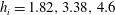 $h_{i}=1.82,3.38,4.6$
mm, and
$h_{i}=1.82,3.38,4.6$
mm, and
 ${\it\theta}=23.7^{\circ }$
and
${\it\theta}=23.7^{\circ }$
and
 $h_{i}=1.5,2.5,5$
mm. Note that the model does not take into account the effect of removing the gate during the initial instants even though it has a non-negligible impact on the flow dynamics as shown in Ionescu et al. (Reference Ionescu, Mangeney, Bouchut and Roche2015). For instance, when the gate is taken into account, even with no friction along it, the flow is substantially slowed down; however, the deposit is almost unchanged. All the simulations are performed using 20 layers.
$h_{i}=1.5,2.5,5$
mm. Note that the model does not take into account the effect of removing the gate during the initial instants even though it has a non-negligible impact on the flow dynamics as shown in Ionescu et al. (Reference Ionescu, Mangeney, Bouchut and Roche2015). For instance, when the gate is taken into account, even with no friction along it, the flow is substantially slowed down; however, the deposit is almost unchanged. All the simulations are performed using 20 layers.
We compare hereafter (i) the constant and variable friction rheologies and (ii) the monolayer and multilayer approaches. In table 3, we summarize the notation and symbols used for the different models. MSM is the notation for multilayer models. Note that the monolayer model with a constant friction coefficient (denoted
 ${\it\mu}_{s}$
-monolayer model) corresponds to the Savage–Hutter classical model when
${\it\mu}_{s}$
-monolayer model) corresponds to the Savage–Hutter classical model when
 $K_{act/pas}=1$
. This model is widely used in the literature, e.g. Gray, Tai & Noelle (Reference Gray, Tai and Noelle2003), Mangeney-Castelnau et al. (Reference Mangeney-Castelnau, Bouchut, Vilotte, Lajeunesse, Aubertin and Pirulli2005). Note also that the monolayer model with a variable friction coefficient (denoted
$K_{act/pas}=1$
. This model is widely used in the literature, e.g. Gray, Tai & Noelle (Reference Gray, Tai and Noelle2003), Mangeney-Castelnau et al. (Reference Mangeney-Castelnau, Bouchut, Vilotte, Lajeunesse, Aubertin and Pirulli2005). Note also that the monolayer model with a variable friction coefficient (denoted
 ${\it\mu}(I)$
-monolayer model) corresponds to the one proposed by Pouliquen (Reference Pouliquen1999b
), which has been recently used by Mangeney-Castelnau et al. (Reference Mangeney-Castelnau, Vilotte, Bristeau, Perthame, Bouchut, Simeoni and Yerneni2003) and Mangeney et al. (Reference Mangeney, Bouchut, Thomas, Vilotte and Bristeau2007). This model also coincides with the one proposed in Gray & Edwards (Reference Gray and Edwards2014) by dropping second-order terms, that is, viscous terms.
${\it\mu}(I)$
-monolayer model) corresponds to the one proposed by Pouliquen (Reference Pouliquen1999b
), which has been recently used by Mangeney-Castelnau et al. (Reference Mangeney-Castelnau, Vilotte, Bristeau, Perthame, Bouchut, Simeoni and Yerneni2003) and Mangeney et al. (Reference Mangeney, Bouchut, Thomas, Vilotte and Bristeau2007). This model also coincides with the one proposed in Gray & Edwards (Reference Gray and Edwards2014) by dropping second-order terms, that is, viscous terms.
Table 3. Summary of notation of the different models and colours/symbols.

4.2.3 Deposit profiles
Let us compare the deposits simulated with the
 ${\it\mu}(I)$
-rheology and with a constant friction coefficient
${\it\mu}(I)$
-rheology and with a constant friction coefficient
 ${\it\mu}_{s}$
for different slopes
${\it\mu}_{s}$
for different slopes
 ${\it\theta}$
and erodible bed thicknesses
${\it\theta}$
and erodible bed thicknesses
 $h_{i}$
. Figure 8 shows that the deposit calculated with the variable friction coefficient
$h_{i}$
. Figure 8 shows that the deposit calculated with the variable friction coefficient
 ${\it\mu}(I)$
is closer to the experimental deposit than the one calculated with a constant friction coefficient
${\it\mu}(I)$
is closer to the experimental deposit than the one calculated with a constant friction coefficient
 ${\it\mu}_{s}$
. The runout distance with the constant coefficient
${\it\mu}_{s}$
. The runout distance with the constant coefficient
 ${\it\mu}_{s}$
is always too long except for
${\it\mu}_{s}$
is always too long except for
 ${\it\theta}=19^{\circ }$
and
${\it\theta}=19^{\circ }$
and
 $h_{i}=5.3$
mm (see figure 8
d). To properly reproduce the runout distance with a constant friction coefficient, we need to increase its value. For example, with a slope
$h_{i}=5.3$
mm (see figure 8
d). To properly reproduce the runout distance with a constant friction coefficient, we need to increase its value. For example, with a slope
 ${\it\theta}=16^{\circ }$
and an erodible bed thickness
${\it\theta}=16^{\circ }$
and an erodible bed thickness
 $h_{i}=2.5$
mm (figure 8
a), we need to use the value
$h_{i}=2.5$
mm (figure 8
a), we need to use the value
 ${\it\mu}_{s}=\tan (27.3^{\circ })$
to produce the runout observed in the laboratory experiments. That means an increment of 0.039 in the
${\it\mu}_{s}=\tan (27.3^{\circ })$
to produce the runout observed in the laboratory experiments. That means an increment of 0.039 in the
 ${\it\mu}_{s}$
value. These results are consistent with the simulations of Ionescu et al. (Reference Ionescu, Mangeney, Bouchut and Roche2015), showing that the runout is strongly overestimated when the viscosity tends to zero (i.e. when
${\it\mu}_{s}$
value. These results are consistent with the simulations of Ionescu et al. (Reference Ionescu, Mangeney, Bouchut and Roche2015), showing that the runout is strongly overestimated when the viscosity tends to zero (i.e. when
 ${\it\mu}$
tends to
${\it\mu}$
tends to
 ${\it\mu}_{s}$
).
${\it\mu}_{s}$
).

Figure 8. Deposit obtained in the experiments (solid-circle blue line), with the
 ${\it\mu}_{s}$
-MSM (dotted-circle red line) and with the
${\it\mu}_{s}$
-MSM (dotted-circle red line) and with the
 ${\it\mu}(I)$
-MSM (solid-cross green line), for different slopes
${\it\mu}(I)$
-MSM (solid-cross green line), for different slopes
 ${\it\theta}$
and erodible bed thicknesses
${\it\theta}$
and erodible bed thicknesses
 $h_{i}$
.
$h_{i}$
.

Figure 9. Deposit obtained in the experiments (solid-circle blue line), with the
 ${\it\mu}_{s}$
-MSM (dotted-circle red line), the
${\it\mu}_{s}$
-MSM (dotted-circle red line), the
 ${\it\mu}(I)$
-MSM (solid-cross green line), the
${\it\mu}(I)$
-MSM (solid-cross green line), the
 ${\it\mu}_{s}$
-monolayer model (dashed red line) and with the
${\it\mu}_{s}$
-monolayer model (dashed red line) and with the
 ${\it\mu}(I)$
-monolayer model (solid green line) for a slope
${\it\mu}(I)$
-monolayer model (solid green line) for a slope
 ${\it\theta}=22^{\circ }$
and an erodible bed thickness
${\it\theta}=22^{\circ }$
and an erodible bed thickness
 $h_{i}=1.82$
mm. Circled sections indicate specific locations for data shown in figure 10.
$h_{i}=1.82$
mm. Circled sections indicate specific locations for data shown in figure 10.
Figure 9 shows, for a slope
 ${\it\theta}=22^{\circ }$
and
${\it\theta}=22^{\circ }$
and
 $h_{i}=1.82$
mm, the final deposit obtained using the constant or variable friction coefficients for multilayer and monolayer models. The difference between the multilayer and monolayer models is stronger when using the
$h_{i}=1.82$
mm, the final deposit obtained using the constant or variable friction coefficients for multilayer and monolayer models. The difference between the multilayer and monolayer models is stronger when using the
 ${\it\mu}(I)$
-rheology. For instance, the multilayer approach changes the full deposit profiles for the
${\it\mu}(I)$
-rheology. For instance, the multilayer approach changes the full deposit profiles for the
 ${\it\mu}(I)$
-rheology, while it only changes the front position for
${\it\mu}(I)$
-rheology, while it only changes the front position for
 ${\it\mu}_{s}$
. The multilayer approach makes it possible to obtain a deposit shape which is very close to the experiments with the
${\it\mu}_{s}$
. The multilayer approach makes it possible to obtain a deposit shape which is very close to the experiments with the
 ${\it\mu}(I)$
-rheology. More generally, the shape of the deposit is closer to the observations with
${\it\mu}(I)$
-rheology. More generally, the shape of the deposit is closer to the observations with
 ${\it\mu}(I)$
-MSM than with
${\it\mu}(I)$
-MSM than with
 ${\it\mu}_{s}$
-MSM.
${\it\mu}_{s}$
-MSM.
4.2.4 Effect of the erodible bed
Figure 10 shows two zooms, one near the maximum thickness of the deposit (zone of circle (I) in figure 9), and one near the front (zone of circle (II) in figure 9), for
 ${\it\theta}=22^{\circ }$
and different values of
${\it\theta}=22^{\circ }$
and different values of
 $h_{i}$
. With the
$h_{i}$
. With the
 ${\it\mu}(I)$
-MSM, the runout distance
${\it\mu}(I)$
-MSM, the runout distance
 $r_{f}$
increases as the thickness of the erodible bed
$r_{f}$
increases as the thickness of the erodible bed
 $h_{i}$
increases (figure 10
a (II)) as observed in laboratory experiments. On the contrary, with the
$h_{i}$
increases (figure 10
a (II)) as observed in laboratory experiments. On the contrary, with the
 ${\it\mu}_{s}$
-MSM (figure 10
b (II)), the runout distance
${\it\mu}_{s}$
-MSM (figure 10
b (II)), the runout distance
 $r_{f}$
decreases with increasing
$r_{f}$
decreases with increasing
 $h_{i}$
. Note that in both cases the maximum final thickness
$h_{i}$
. Note that in both cases the maximum final thickness
 $h_{f}$
decreases with increasing
$h_{f}$
decreases with increasing
 $h_{i}$
as it occurs in the experiments (figure 10
a (I),b (I)).
$h_{i}$
as it occurs in the experiments (figure 10
a (I),b (I)).

Figure 10. Influence of the thickness of the erodible bed on the runout distance
 $r_{f}$
and on the maximum final thickness
$r_{f}$
and on the maximum final thickness
 $h_{f}$
(inset graphs) with the
$h_{f}$
(inset graphs) with the
 ${\it\mu}(I)$
-MSM (a) and with the
${\it\mu}(I)$
-MSM (a) and with the
 ${\it\mu}_{s}$
-MSM (b), for a slope
${\it\mu}_{s}$
-MSM (b), for a slope
 ${\it\theta}=22^{\circ }$
, in zones marked with circles in figure 9.
${\it\theta}=22^{\circ }$
, in zones marked with circles in figure 9.
Figure 11 shows that the decrease in runout distance with increasing
 $h_{i}$
for constant friction
$h_{i}$
for constant friction
 ${\it\mu}_{s}$
is observed for all slopes, e.g.
${\it\mu}_{s}$
is observed for all slopes, e.g.
 ${\it\theta}=0^{\circ },10^{\circ },16^{\circ },19^{\circ },22^{\circ }$
and
${\it\theta}=0^{\circ },10^{\circ },16^{\circ },19^{\circ },22^{\circ }$
and
 $23.7^{\circ }$
. For the constant friction coefficient case, the
$23.7^{\circ }$
. For the constant friction coefficient case, the
 ${\it\mu}_{s}$
-MSM and
${\it\mu}_{s}$
-MSM and
 ${\it\mu}_{s}$
-monolayer models follow the same trend. Note that this non-physical decrease in runout distance with increasing
${\it\mu}_{s}$
-monolayer models follow the same trend. Note that this non-physical decrease in runout distance with increasing
 $h_{i}$
has been demonstrated analytically in Faccanoni & Mangeney (Reference Faccanoni and Mangeney2013) for the monolayer model. Moreover, laboratory experiments show that when the thickness of the erodible bed increases, for slopes
$h_{i}$
has been demonstrated analytically in Faccanoni & Mangeney (Reference Faccanoni and Mangeney2013) for the monolayer model. Moreover, laboratory experiments show that when the thickness of the erodible bed increases, for slopes
 ${\it\theta}\geqslant {\it\theta}_{c}$
, where
${\it\theta}\geqslant {\it\theta}_{c}$
, where
 ${\it\theta}_{c}\in [12^{\circ },16^{\circ }]$
is a critical slope, the runout distance
${\it\theta}_{c}\in [12^{\circ },16^{\circ }]$
is a critical slope, the runout distance
 $r_{f}$
and the stopping time
$r_{f}$
and the stopping time
 $t_{f}$
both increase while the maximum final thickness
$t_{f}$
both increase while the maximum final thickness
 $h_{f}$
decreases. Note that there is no pattern concerning the runout when the thickness
$h_{f}$
decreases. Note that there is no pattern concerning the runout when the thickness
 $h_{i}$
is increased for slopes
$h_{i}$
is increased for slopes
 ${\it\theta}<{\it\theta}_{c}$
(
${\it\theta}<{\it\theta}_{c}$
(
 ${\it\theta}=0^{\circ },10^{\circ }$
) in the laboratory experiments.
${\it\theta}=0^{\circ },10^{\circ }$
) in the laboratory experiments.

Figure 11. Influence of the thickness
 $h_{i}$
of the erodible bed on the final runout
$h_{i}$
of the erodible bed on the final runout
 $r_{f}$
for slopes
$r_{f}$
for slopes
 ${\it\theta}=0^{\circ },10^{\circ },16^{\circ },19^{\circ },22^{\circ }$
and
${\it\theta}=0^{\circ },10^{\circ },16^{\circ },19^{\circ },22^{\circ }$
and
 $23.7^{\circ }$
observed in the experiments of Mangeney et al. (Reference Mangeney, Roche, Hungr, Mangold, Faccanoni and Lucas2010) (solid-circle blue line) and obtained with different simulations using the
$23.7^{\circ }$
observed in the experiments of Mangeney et al. (Reference Mangeney, Roche, Hungr, Mangold, Faccanoni and Lucas2010) (solid-circle blue line) and obtained with different simulations using the
 ${\it\mu}_{s}$
-MSM, with 20 layers (dotted-circle red line) and the
${\it\mu}_{s}$
-MSM, with 20 layers (dotted-circle red line) and the
 ${\it\mu}_{s}$
-monolayer model, i.e. the Savage–Hutter model (dashed red line). There is no laboratory data for
${\it\mu}_{s}$
-monolayer model, i.e. the Savage–Hutter model (dashed red line). There is no laboratory data for
 ${\it\theta}=23.7^{\circ }$
. Normalization is made using
${\it\theta}=23.7^{\circ }$
. Normalization is made using
 $h_{0}=14$
cm.
$h_{0}=14$
cm.
Figure 12 shows that the increase of runout distance observed in the experiments for increasing
 $h_{i}$
is qualitatively well reproduced with the
$h_{i}$
is qualitatively well reproduced with the
 ${\it\mu}(I)$
-MSM. With the
${\it\mu}(I)$
-MSM. With the
 ${\it\mu}(I)$
-MSM, the runout increase with
${\it\mu}(I)$
-MSM, the runout increase with
 $h_{i}$
is actually larger for higher slopes, as observed experimentally: at
$h_{i}$
is actually larger for higher slopes, as observed experimentally: at
 ${\it\theta}=16^{\circ }$
, the runout distance is almost unaffected by the thickness of the erodible bed while it increases by 26.9 % at
${\it\theta}=16^{\circ }$
, the runout distance is almost unaffected by the thickness of the erodible bed while it increases by 26.9 % at
 ${\it\theta}=22^{\circ }$
when the thickness of the erodible bed increase from 1.82 to 4.6 mm. Note that in the
${\it\theta}=22^{\circ }$
when the thickness of the erodible bed increase from 1.82 to 4.6 mm. Note that in the
 ${\it\mu}(I)$
-MSM, the increase of the runout distance appears on slopes
${\it\mu}(I)$
-MSM, the increase of the runout distance appears on slopes
 ${\it\theta}>16^{\circ }$
, higher than
${\it\theta}>16^{\circ }$
, higher than
 ${\it\theta}_{c}$
in the experiments. Actually, it appears starting with the slope
${\it\theta}_{c}$
in the experiments. Actually, it appears starting with the slope
 ${\it\theta}=18^{\circ }$
. When using the
${\it\theta}=18^{\circ }$
. When using the
 ${\it\mu}(I)$
-monolayer model, the runout distance is higher than for the
${\it\mu}(I)$
-monolayer model, the runout distance is higher than for the
 ${\it\mu}(I)$
-MSM whatever the slope and thickness of the erodible bed. Based on the values of the runout distance in these cases, it is hard to discriminate which of the monolayer or multilayer models is closer to the experiments. However, in the
${\it\mu}(I)$
-MSM whatever the slope and thickness of the erodible bed. Based on the values of the runout distance in these cases, it is hard to discriminate which of the monolayer or multilayer models is closer to the experiments. However, in the
 ${\it\mu}(I)$
-monolayer model, the runout distance at
${\it\mu}(I)$
-monolayer model, the runout distance at
 ${\it\theta}=16^{\circ }$
and
${\it\theta}=16^{\circ }$
and
 $19^{\circ }$
decreases when
$19^{\circ }$
decreases when
 $h_{i}$
increases, contrary to the experimental data. For
$h_{i}$
increases, contrary to the experimental data. For
 ${\it\theta}=22^{\circ }$
and
${\it\theta}=22^{\circ }$
and
 ${\it\theta}=23.7^{\circ }$
, the monolayer and multilayer
${\it\theta}=23.7^{\circ }$
, the monolayer and multilayer
 ${\it\mu}(I)$
models reproduce qualitatively the increase in runout with
${\it\mu}(I)$
models reproduce qualitatively the increase in runout with
 $h_{i}$
. Note that for
$h_{i}$
. Note that for
 ${\it\theta}=0^{\circ },10^{\circ }$
(
${\it\theta}=0^{\circ },10^{\circ }$
(
 ${\it\theta}<{\it\theta}_{c}$
), the
${\it\theta}<{\it\theta}_{c}$
), the
 ${\it\mu}(I)$
models predict a very slight decrease in the runout distance.
${\it\mu}(I)$
models predict a very slight decrease in the runout distance.
The
 ${\it\mu}(I)$
-MSM is the model corresponding to the multilayer approach with the
${\it\mu}(I)$
-MSM is the model corresponding to the multilayer approach with the
 ${\it\mu}(I)$
-rheology when
${\it\mu}(I)$
-rheology when
 $\Vert \unicode[STIX]{x1D63F}(\boldsymbol{u})\Vert$
is approximated by the main term in (4.7), and
$\Vert \unicode[STIX]{x1D63F}(\boldsymbol{u})\Vert$
is approximated by the main term in (4.7), and
 ${\it\mu}(I)$
-C-MSM when
${\it\mu}(I)$
-C-MSM when
 $\Vert \unicode[STIX]{x1D63F}(\boldsymbol{u})\Vert$
is approximated by the correction (4.8). Figure 12 shows that the correction of
$\Vert \unicode[STIX]{x1D63F}(\boldsymbol{u})\Vert$
is approximated by the correction (4.8). Figure 12 shows that the correction of
 $\Vert \unicode[STIX]{x1D63F}(\boldsymbol{u})\Vert$
corresponding to
$\Vert \unicode[STIX]{x1D63F}(\boldsymbol{u})\Vert$
corresponding to
 ${\it\mu}(I)$
-C-MSM improves the simulation of both the runout extent and the influence of the erodible bed. They both increase the runout when
${\it\mu}(I)$
-C-MSM improves the simulation of both the runout extent and the influence of the erodible bed. They both increase the runout when
 $h_{i}$
increases, although the effect of erosion is still much smaller than in the experiments.
$h_{i}$
increases, although the effect of erosion is still much smaller than in the experiments.
For example, for
 ${\it\theta}=19^{\circ }$
, when
${\it\theta}=19^{\circ }$
, when
 $h_{i}$
varies from 1.5 to 5.3 mm, the experimental runout increases by 15.1 %. On the contrary, for the monolayer model the runout decreases by 1.1 %. For the
$h_{i}$
varies from 1.5 to 5.3 mm, the experimental runout increases by 15.1 %. On the contrary, for the monolayer model the runout decreases by 1.1 %. For the
 ${\it\mu}(I)$
-MSM the runout increases by 2.5 %, and for the
${\it\mu}(I)$
-MSM the runout increases by 2.5 %, and for the
 ${\it\mu}(I)$
-C-MSM it increases by 6.8 %. For
${\it\mu}(I)$
-C-MSM it increases by 6.8 %. For
 ${\it\theta}=22^{\circ }$
, when
${\it\theta}=22^{\circ }$
, when
 $h_{i}$
varies from 1.82 to 4.6 mm, the experimental runout increases by 26.9 %. It increases by 2.2 %, 4.4 % and 8.6 % for the monolayer model, the
$h_{i}$
varies from 1.82 to 4.6 mm, the experimental runout increases by 26.9 %. It increases by 2.2 %, 4.4 % and 8.6 % for the monolayer model, the
 ${\it\mu}(I)$
-MSM and the
${\it\mu}(I)$
-MSM and the
 ${\it\mu}(I)$
-C-MSM, respectively.
${\it\mu}(I)$
-C-MSM, respectively.
In figure 13, the final time (time at which the front stops) is plotted as a function of the thickness of the erodible bed for
 ${\it\theta}=16^{\circ }$
,
${\it\theta}=16^{\circ }$
,
 ${\it\theta}=19^{\circ }$
and
${\it\theta}=19^{\circ }$
and
 ${\it\theta}=22^{\circ }$
. Moreover, for
${\it\theta}=22^{\circ }$
. Moreover, for
 ${\it\theta}=22^{\circ }$
, we also plot the experimental data. Experimental data show that the final time increases when the thickness of the erodible bed increases. We can see that this is true for all the values of
${\it\theta}=22^{\circ }$
, we also plot the experimental data. Experimental data show that the final time increases when the thickness of the erodible bed increases. We can see that this is true for all the values of
 ${\it\theta}$
for the multilayer method. However, we observe that it is only true for the highest value,
${\it\theta}$
for the multilayer method. However, we observe that it is only true for the highest value,
 ${\it\theta}=22^{\circ }$
, in the case of the monolayer model, whereas the final time decreases when the erodible bed increases for
${\it\theta}=22^{\circ }$
, in the case of the monolayer model, whereas the final time decreases when the erodible bed increases for
 ${\it\theta}=16^{\circ }$
and
${\it\theta}=16^{\circ }$
and
 ${\it\theta}=19^{\circ }$
.
${\it\theta}=19^{\circ }$
.

Figure 12. Influence of the thickness
 $h_{i}$
of the erodible bed on the final runout
$h_{i}$
of the erodible bed on the final runout
 $r_{f}$
for slopes
$r_{f}$
for slopes
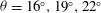 ${\it\theta}=16^{\circ },19^{\circ },22^{\circ }$
and
${\it\theta}=16^{\circ },19^{\circ },22^{\circ }$
and
 $23.7^{\circ }$
observed in the experiments of Mangeney et al. (Reference Mangeney, Roche, Hungr, Mangold, Faccanoni and Lucas2010) (solid-circle blue line) and obtained with different simulations using the
$23.7^{\circ }$
observed in the experiments of Mangeney et al. (Reference Mangeney, Roche, Hungr, Mangold, Faccanoni and Lucas2010) (solid-circle blue line) and obtained with different simulations using the
 ${\it\mu}(I)$
-MSM, with 20 layers (solid-cross green line), with the
${\it\mu}(I)$
-MSM, with 20 layers (solid-cross green line), with the
 ${\it\mu}(I)$
-monolayer model (solid green line) and with the
${\it\mu}(I)$
-monolayer model (solid green line) and with the
 ${\it\mu}(I)$
-C-MSM (dashed black line). There is no laboratory data for
${\it\mu}(I)$
-C-MSM (dashed black line). There is no laboratory data for
 ${\it\theta}=23.7^{\circ }$
. Normalization is made using
${\it\theta}=23.7^{\circ }$
. Normalization is made using
 $h_{0}=14$
cm.
$h_{0}=14$
cm.

Figure 13. Influence of the thickness
 $h_{i}$
of the erodible bed on the final time
$h_{i}$
of the erodible bed on the final time
 $t_{f}$
for slopes
$t_{f}$
for slopes
 ${\it\theta}=16^{\circ },19^{\circ }$
and
${\it\theta}=16^{\circ },19^{\circ }$
and
 $22^{\circ }$
by using the
$22^{\circ }$
by using the
 ${\it\mu}(I)$
-MSM with 20 layers (solid-cross green line), the
${\it\mu}(I)$
-MSM with 20 layers (solid-cross green line), the
 ${\it\mu}(I)$
-monolayer model (solid green line) and the values observed in the experiments of Mangeney et al. (Reference Mangeney, Roche, Hungr, Mangold, Faccanoni and Lucas2010) for slope
${\it\mu}(I)$
-monolayer model (solid green line) and the values observed in the experiments of Mangeney et al. (Reference Mangeney, Roche, Hungr, Mangold, Faccanoni and Lucas2010) for slope
 ${\it\theta}=22^{\circ }$
(solid-circle blue line). Normalization is made using
${\it\theta}=22^{\circ }$
(solid-circle blue line). Normalization is made using
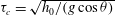 ${\it\tau}_{c}=\sqrt{h_{0}/(g\cos {\it\theta})}$
and
${\it\tau}_{c}=\sqrt{h_{0}/(g\cos {\it\theta})}$
and
 $h_{0}=14$
cm.
$h_{0}=14$
cm.
4.2.5 Flow dynamics and velocity profiles
Figures 14 and 15 show the time evolution of the granular column thickness for a slope
 ${\it\theta}=22^{\circ }$
and an erodible bed of thickness
${\it\theta}=22^{\circ }$
and an erodible bed of thickness
 $h_{i}=1.82$
mm for
$h_{i}=1.82$
mm for
 ${\it\mu}_{s}$
and
${\it\mu}_{s}$
and
 ${\it\mu}(I)$
, respectively, for both the monolayer and multilayer models. As observed for the deposit, the difference between the thickness profiles simulated with the multilayer and the monolayer model is stronger for
${\it\mu}(I)$
, respectively, for both the monolayer and multilayer models. As observed for the deposit, the difference between the thickness profiles simulated with the multilayer and the monolayer model is stronger for
 ${\it\mu}(I)$
than for
${\it\mu}(I)$
than for
 ${\it\mu}_{s}$
. The
${\it\mu}_{s}$
. The
 ${\it\mu}(I)$
-MSM makes it possible to increase the maximum thickness of the flow and decrease the thickness of the front. This is an important result as the shape of the front may be an indicator of the flow rheology (Pouliquen Reference Pouliquen1999a
; Jessop et al.
Reference Jessop, Kelfoun, Labazuy, Mangeney, Roche, Tillier, Trouillet and Thibault2012).
${\it\mu}(I)$
-MSM makes it possible to increase the maximum thickness of the flow and decrease the thickness of the front. This is an important result as the shape of the front may be an indicator of the flow rheology (Pouliquen Reference Pouliquen1999a
; Jessop et al.
Reference Jessop, Kelfoun, Labazuy, Mangeney, Roche, Tillier, Trouillet and Thibault2012).

Figure 14. Thickness of the granular mass at different times in the experiments (solid-circle blue line), with the
 ${\it\mu}_{s}$
-MSM with 20 layers (dotted-circle red line), with the
${\it\mu}_{s}$
-MSM with 20 layers (dotted-circle red line), with the
 ${\it\mu}_{s}$
-monolayer model (Savage–Hutter model, dashed red line) and with the flow/non-flow interface (dashed brown line), for the slope
${\it\mu}_{s}$
-monolayer model (Savage–Hutter model, dashed red line) and with the flow/non-flow interface (dashed brown line), for the slope
 ${\it\theta}=22^{\circ }$
and erodible bed thickness
${\it\theta}=22^{\circ }$
and erodible bed thickness
 $h_{i}=1.82$
mm.
$h_{i}=1.82$
mm.
When a constant coefficient
 ${\it\mu}_{s}$
is used, very similar profiles are obtained with the
${\it\mu}_{s}$
is used, very similar profiles are obtained with the
 ${\it\mu}_{s}$
-MSM and
${\it\mu}_{s}$
-MSM and
 ${\it\mu}_{s}$
-monolayer model (Savage–Hutter model). As a result, the multilayer approach does not significantly improve the results when a constant friction coefficient is used. Note that during the initial instants, the simulated mass spreads faster than in the experiments. This is partly due to the role of initial gate removal that is not taken into account here. However, this effect does not explain the strong difference between the simulation and experiments (see Ionescu et al.
Reference Ionescu, Mangeney, Bouchut and Roche2015 for more details). The hydrostatic assumption may also be responsible for this overestimation of the spreading velocity (see e.g. Mangeney-Castelnau et al.
Reference Mangeney-Castelnau, Bouchut, Vilotte, Lajeunesse, Aubertin and Pirulli2005). In these figures we also show the flow/no-flow interfaces computed with the multilayer models
${\it\mu}_{s}$
-monolayer model (Savage–Hutter model). As a result, the multilayer approach does not significantly improve the results when a constant friction coefficient is used. Note that during the initial instants, the simulated mass spreads faster than in the experiments. This is partly due to the role of initial gate removal that is not taken into account here. However, this effect does not explain the strong difference between the simulation and experiments (see Ionescu et al.
Reference Ionescu, Mangeney, Bouchut and Roche2015 for more details). The hydrostatic assumption may also be responsible for this overestimation of the spreading velocity (see e.g. Mangeney-Castelnau et al.
Reference Mangeney-Castelnau, Bouchut, Vilotte, Lajeunesse, Aubertin and Pirulli2005). In these figures we also show the flow/no-flow interfaces computed with the multilayer models
 ${\it\mu}_{s}$
-MSM,
${\it\mu}_{s}$
-MSM,
 ${\it\mu}(I)$
-MSM and
${\it\mu}(I)$
-MSM and
 ${\it\mu}(I)$
-C-MSM, by considering a threshold velocity of
${\it\mu}(I)$
-C-MSM, by considering a threshold velocity of
 $0.001~\text{m}~\text{s}^{-1}$
to compute these interfaces. We see in figure 14 that the flow/no-flow interface has a step-like shape for
$0.001~\text{m}~\text{s}^{-1}$
to compute these interfaces. We see in figure 14 that the flow/no-flow interface has a step-like shape for
 ${\it\mu}_{s}$
-MSM while it has a smoother shape for
${\it\mu}_{s}$
-MSM while it has a smoother shape for
 ${\it\mu}(I)$
-MSM (see figure 15) in better qualitative agreement with laboratory experiments and numerical modelling solving the full Navier–Stokes equations (e.g. figures 9 and 18 of Ionescu et al.
Reference Ionescu, Mangeney, Bouchut and Roche2015). The flow/no-flow interface in the uppermost part even seems to be improved when using
${\it\mu}(I)$
-MSM (see figure 15) in better qualitative agreement with laboratory experiments and numerical modelling solving the full Navier–Stokes equations (e.g. figures 9 and 18 of Ionescu et al.
Reference Ionescu, Mangeney, Bouchut and Roche2015). The flow/no-flow interface in the uppermost part even seems to be improved when using
 ${\it\mu}(I)$
-C-MSM. For
${\it\mu}(I)$
-C-MSM. For
 ${\it\mu}(I)$
-MSM and
${\it\mu}(I)$
-MSM and
 ${\it\mu}(I)$
-C-MSM, the lower layers stop before the upper layers as observed experimentally. Note that in figures 14 and 15 we do not see the flow/no-flow interface at the final time because the material has already stopped. As was shown in § 4.1.1, the wall friction effect is crucial to determine the position of the flow/no-flow interface. Because in this test we do not consider the exact definition of the wall friction term, as in Ionescu et al. (Reference Ionescu, Mangeney, Bouchut and Roche2015), the flow/no-flow interface should not be very well captured.
${\it\mu}(I)$
-C-MSM, the lower layers stop before the upper layers as observed experimentally. Note that in figures 14 and 15 we do not see the flow/no-flow interface at the final time because the material has already stopped. As was shown in § 4.1.1, the wall friction effect is crucial to determine the position of the flow/no-flow interface. Because in this test we do not consider the exact definition of the wall friction term, as in Ionescu et al. (Reference Ionescu, Mangeney, Bouchut and Roche2015), the flow/no-flow interface should not be very well captured.

Figure 15. Thickness of the granular mass at different times in the experiments (solid-circle blue line), with the
 ${\it\mu}(I)$
-MSM using 20 layers (solid-cross green line), with the
${\it\mu}(I)$
-MSM using 20 layers (solid-cross green line), with the
 ${\it\mu}(I)$
-monolayer model (solid green line), with the
${\it\mu}(I)$
-monolayer model (solid green line), with the
 ${\it\mu}(I)$
-C-MSM (dashed black line), and the flow/non-flow interface with both multilayer models (dashed brown/solid brown lines) for the slope
${\it\mu}(I)$
-C-MSM (dashed black line), and the flow/non-flow interface with both multilayer models (dashed brown/solid brown lines) for the slope
 ${\it\theta}=22^{\circ }$
and erodible bed thickness
${\it\theta}=22^{\circ }$
and erodible bed thickness
 $h_{i}=1.82$
mm.
$h_{i}=1.82$
mm.
Figure 16 shows that the second-order correction in
 ${\it\mu}(I)$
-C-MSM leads to simulated deposits that are generally closer to the experimental observations than those calculated with
${\it\mu}(I)$
-C-MSM leads to simulated deposits that are generally closer to the experimental observations than those calculated with
 ${\it\mu}(I)$
-MSM. In particular, the deposits at
${\it\mu}(I)$
-MSM. In particular, the deposits at
 ${\it\theta}=19^{\circ }$
and
${\it\theta}=19^{\circ }$
and
 ${\it\theta}=22^{\circ }$
with
${\it\theta}=22^{\circ }$
with
 $h_{i}=4.6$
mm are very well reproduced (figure 16
b,c,d,f). However, in some cases,
$h_{i}=4.6$
mm are very well reproduced (figure 16
b,c,d,f). However, in some cases,
 ${\it\mu}(I)$
-MSM gives better results than
${\it\mu}(I)$
-MSM gives better results than
 ${\it\mu}(I)$
-C-MSM, for example for
${\it\mu}(I)$
-C-MSM, for example for
 ${\it\theta}=22^{\circ }$
with
${\it\theta}=22^{\circ }$
with
 $h_{i}=1.82$
mm. This is true for the overall dynamics as illustrated in figure 15 that shows the time change of the granular column thickness. We can see that with
$h_{i}=1.82$
mm. This is true for the overall dynamics as illustrated in figure 15 that shows the time change of the granular column thickness. We can see that with
 ${\it\mu}(I)$
-C-MSM, the avalanche is faster and the runout is overestimated and very similar to the runout obtained with the
${\it\mu}(I)$
-C-MSM, the avalanche is faster and the runout is overestimated and very similar to the runout obtained with the
 ${\it\mu}(I)$
monolayer model. As other second-order terms than those included in the
${\it\mu}(I)$
monolayer model. As other second-order terms than those included in the
 ${\it\mu}(I)$
-C-MSM model are neglected, it is not easy to draw a firm conclusion on the improvement of results when using second-order terms.
${\it\mu}(I)$
-C-MSM model are neglected, it is not easy to draw a firm conclusion on the improvement of results when using second-order terms.

Figure 16. Simulated deposits at different slopes
 ${\it\theta}$
and erodible bed thicknesses
${\it\theta}$
and erodible bed thicknesses
 $h_{i}$
with the
$h_{i}$
with the
 ${\it\mu}(I)$
-C-MSM (dashed black line) and the
${\it\mu}(I)$
-C-MSM (dashed black line) and the
 ${\it\mu}(I)$
-MSM (solid-cross green line). The deposits observed in the experiments are represented by solid-circle blue lines.
${\it\mu}(I)$
-MSM (solid-cross green line). The deposits observed in the experiments are represented by solid-circle blue lines.
The multilayer approach makes it possible to obtain a normal profile of the downslope velocity. Figures 17 and 18 show the normal profiles of the downslope velocity obtained at different times until the mass stops, for two different configurations of slopes and erodible beds. In order to obtain a more accurate profile, 40 layers are used in the
 ${\it\mu}(I)$
-MSM. The different kind of profiles observed in figures 17 and 18 are in good qualitative agreement with typical velocity profiles of granular flows GDR MiDi (2004) (see also Lusso et al.
Reference Lusso, Bouchut, Ern and Mangeney2015a
and Lusso et al.
Reference Lusso, Ern, Bouchut, Mangeney, Farin and Roche2015b
), from Bagnold-like to S-shaped profiles. This shows the ability of the model to recover velocity profiles in a wide range of regimes.
${\it\mu}(I)$
-MSM. The different kind of profiles observed in figures 17 and 18 are in good qualitative agreement with typical velocity profiles of granular flows GDR MiDi (2004) (see also Lusso et al.
Reference Lusso, Bouchut, Ern and Mangeney2015a
and Lusso et al.
Reference Lusso, Ern, Bouchut, Mangeney, Farin and Roche2015b
), from Bagnold-like to S-shaped profiles. This shows the ability of the model to recover velocity profiles in a wide range of regimes.
Finally, let us compare the averaged velocity obtained with the
 ${\it\mu}(I)$
-monolayer model to the average of the velocities over all the layers in the
${\it\mu}(I)$
-monolayer model to the average of the velocities over all the layers in the
 ${\it\mu}(I)$
-MSM. In figure 17, for the green profile (respectively red and magenta profiles), the velocity in the monolayer model is
${\it\mu}(I)$
-MSM. In figure 17, for the green profile (respectively red and magenta profiles), the velocity in the monolayer model is
 $1.01~\text{m}~\text{s}^{-1}$
(respectively 0.02 and
$1.01~\text{m}~\text{s}^{-1}$
(respectively 0.02 and
 $0.14~\text{m}~\text{s}^{-1}$
) and it is
$0.14~\text{m}~\text{s}^{-1}$
) and it is
 $0.95~\text{m}~\text{s}^{-1}$
in the multilayer model (respectively 0.03 and
$0.95~\text{m}~\text{s}^{-1}$
in the multilayer model (respectively 0.03 and
 $0.05~\text{m}~\text{s}^{-1}$
). Note that we obtain similar values for the first and second profiles. For the third profile, the averaged velocities strongly differ. Actually, at this position and time, the velocity profile corresponds to the stopping phase for the multilayer model but not for the monolayer model. As a result, the velocity obtained in the multilayer model is lower than that obtained in the monolayer model. Figure 19 shows the normal profile of normal velocity for the same configuration as figure 17. Note that the normal velocities are always negative and that their absolute values are greater in the upper layers.
$0.05~\text{m}~\text{s}^{-1}$
). Note that we obtain similar values for the first and second profiles. For the third profile, the averaged velocities strongly differ. Actually, at this position and time, the velocity profile corresponds to the stopping phase for the multilayer model but not for the monolayer model. As a result, the velocity obtained in the multilayer model is lower than that obtained in the monolayer model. Figure 19 shows the normal profile of normal velocity for the same configuration as figure 17. Note that the normal velocities are always negative and that their absolute values are greater in the upper layers.

Figure 17. Normal profiles of the downslope velocity obtained with the
 ${\it\mu}(I)$
-MSM (40 layers) for
${\it\mu}(I)$
-MSM (40 layers) for
 ${\it\theta}=22^{\circ }$
and
${\it\theta}=22^{\circ }$
and
 $h_{i}=1.82$
mm during granular collapse at different positions (
$h_{i}=1.82$
mm during granular collapse at different positions (
 $x=0.095,0.495,0.995$
m). For these positions, we represent the velocity profiles for different times, taken every 0.15 s (blue lines). The first selected profile (green) shows a profile at the beginning of the flow and the second (red) and third (magenta) profiles were measured during the stopping stage. The final deposit is represented by the solid brown line.
$x=0.095,0.495,0.995$
m). For these positions, we represent the velocity profiles for different times, taken every 0.15 s (blue lines). The first selected profile (green) shows a profile at the beginning of the flow and the second (red) and third (magenta) profiles were measured during the stopping stage. The final deposit is represented by the solid brown line.

Figure 18. Normal profiles of the downslope velocity obtained with the
 ${\it\mu}(I)$
-MSM (40 layers) for
${\it\mu}(I)$
-MSM (40 layers) for
 ${\it\theta}=0^{\circ }$
and
${\it\theta}=0^{\circ }$
and
 $h_{i}=1.5$
mm during granular collapse at different positions (
$h_{i}=1.5$
mm during granular collapse at different positions (
 $x=0.045,0.245$
m) and times taken every 0.05 s.
$x=0.045,0.245$
m) and times taken every 0.05 s.

Figure 19. Normal profiles of the normal velocity obtained with the
 ${\it\mu}(I)$
-MSM (40 layers) for
${\it\mu}(I)$
-MSM (40 layers) for
 ${\it\theta}=22^{\circ }$
and for
${\it\theta}=22^{\circ }$
and for
 $h_{i}=1.82$
mm during granular collapse at different positions (
$h_{i}=1.82$
mm during granular collapse at different positions (
 $x=0.095,0.495,0.995$
m) and times taken every 0.2 s.
$x=0.095,0.495,0.995$
m) and times taken every 0.2 s.
5 Conclusions
In this work, we have proposed a multilayer shallow model (MSM) for dry granular flows that considers a
 ${\it\mu}(I)$
-rheology. The multilayer approach has been applied as in Fernández-Nieto et al. (Reference Fernández-Nieto, Koné and Chacón Rebollo2014), thus leading to a solution of the resulting model that is a particular weak solution of the full Navier–Stokes equations with the
${\it\mu}(I)$
-rheology. The multilayer approach has been applied as in Fernández-Nieto et al. (Reference Fernández-Nieto, Koné and Chacón Rebollo2014), thus leading to a solution of the resulting model that is a particular weak solution of the full Navier–Stokes equations with the
 ${\it\mu}(I)$
-rheology. A regularization method has been used to avoid the singularity occurring when
${\it\mu}(I)$
-rheology. A regularization method has been used to avoid the singularity occurring when
 $\Vert \unicode[STIX]{x1D63F}(\boldsymbol{u})\Vert$
vanishes. Our multilayer model satisfies a dissipative energy inequality, which is a requirement for a geophysical model to achieve a solution with physical meaning.
$\Vert \unicode[STIX]{x1D63F}(\boldsymbol{u})\Vert$
vanishes. Our multilayer model satisfies a dissipative energy inequality, which is a requirement for a geophysical model to achieve a solution with physical meaning.
The numerical solutions of this model have been compared to the steady uniform Bagnold flow, whose analytical solution is known (Silbert et al. Reference Silbert, Ertaş, Grest, Halsey, Levine and Plimpton2001; GDR MiDi 2004; Lagrée et al. Reference Lagrée, Staron and Popinet2011). The model has also been compared with analytical solution and laboratory experiments of granular surface flows in narrow channel, where the lateral walls have an important role in the velocity profile (Jop et al. Reference Jop, Forterre and Pouliquen2005, Reference Jop, Forterre and Pouliquen2007). The MSM gives accurate approximations of these tests.
By comparing the numerical results obtained with this new model to laboratory experiments, we have shown that the model qualitatively and sometimes quantitatively reproduces the granular column collapses over inclined erodible beds performed in Mangeney et al. (Reference Mangeney, Roche, Hungr, Mangold, Faccanoni and Lucas2010). The increase of the runout distance with increasing thickness of the erodible bed is only reproduced when using the MSM with the
 ${\it\mu}(I)$
-rheology (
${\it\mu}(I)$
-rheology (
 ${\it\mu}(I)$
-MSM), although this increase is significantly underestimated. To our knowledge, this is the first time that a model has been able to reproduce this effect. The increase in runout distance appears for slopes
${\it\mu}(I)$
-MSM), although this increase is significantly underestimated. To our knowledge, this is the first time that a model has been able to reproduce this effect. The increase in runout distance appears for slopes
 ${\it\theta}\geqslant 18^{\circ }$
whereas it is observed for slopes
${\it\theta}\geqslant 18^{\circ }$
whereas it is observed for slopes
 ${\it\theta}\geqslant 16^{\circ }$
in the laboratory experiments. On the other hand, when using the
${\it\theta}\geqslant 16^{\circ }$
in the laboratory experiments. On the other hand, when using the
 ${\it\mu}(I)$
-monolayer model, the increase of runout distance with the thickness of the erodible bed only occurs for slopes
${\it\mu}(I)$
-monolayer model, the increase of runout distance with the thickness of the erodible bed only occurs for slopes
 ${\it\theta}\geqslant 21^{\circ }$
. Moreover, in the monolayer model for
${\it\theta}\geqslant 21^{\circ }$
. Moreover, in the monolayer model for
 ${\it\theta}=19^{\circ }$
, the runout distance decreases as the thickness of the erodible bed increases, contrary to observations. As a result, when using the
${\it\theta}=19^{\circ }$
, the runout distance decreases as the thickness of the erodible bed increases, contrary to observations. As a result, when using the
 ${\it\mu}(I)$
-rheology, the multilayer model significantly improves the simulated deposits at different slopes over different thicknesses of the erodible bed compared to the monolayer model. In particular it changes the shape of the front. This is an important result as the shape of the front may be an indicator of the flow rheology (Pouliquen Reference Pouliquen1999a
; Jessop et al.
Reference Jessop, Kelfoun, Labazuy, Mangeney, Roche, Tillier, Trouillet and Thibault2012).
${\it\mu}(I)$
-rheology, the multilayer model significantly improves the simulated deposits at different slopes over different thicknesses of the erodible bed compared to the monolayer model. In particular it changes the shape of the front. This is an important result as the shape of the front may be an indicator of the flow rheology (Pouliquen Reference Pouliquen1999a
; Jessop et al.
Reference Jessop, Kelfoun, Labazuy, Mangeney, Roche, Tillier, Trouillet and Thibault2012).
When considering a constant friction coefficient, the multilayer approach only slightly changes the results compared to the monolayer model. Even with the multilayer model, the use of a constant friction coefficient does not make it possible to reproduce the increase in runout distance with increasing thickness of the erodible bed. In fact, the opposite effect is observed. This confirms the analytical results of Faccanoni & Mangeney (Reference Faccanoni and Mangeney2013) obtained for the monolayer Savage–Hutter equations. Furthermore the constant friction model strongly overestimates the front velocity and the runout distances. As a result, simulation of the effect of a thin erodible bed on the granular front dynamics in granular collapses and on their deposits seems to be a good test to discriminate between the different rheologies.
An important result is that this multilayer approach allows us to obtain the normal profiles of the downslope and normal velocities. These profiles qualitatively agree with the typical granular flow profiles during the developed flow and during the stopping phase GDR MiDi (2004). In particular, the model makes it possible to reproduce the change from Bagnold-like to S-shaped velocity profiles, characteristic of flows over a rigid substrate and over a layer of static grains, respectively. As a result, this model should be applicable to a larger range of flow regimes than the depth-averaged models proposed by Capart et al. (Reference Capart, Hung and Stark2015) and Edwards & Gray (Reference Edwards and Gray2015) for which velocity profiles are prescribed.
One of the differences between the multilayer and monolayer approaches is the accuracy of the approximation of the strain rate and consequently of the inertial number and the
 ${\it\mu}(I)$
friction coefficient. We have seen that the
${\it\mu}(I)$
friction coefficient. We have seen that the
 ${\it\mu}(I)$
-C-MSM model, which introduces a second-order correction to improve the approximation of the strain rate, generally improves the results. The increase in runout distance when the thickness of the erodible bed is increased is larger and therefore closer to the laboratory experiments. In addition, the critical slope above which the runout increases with the thickness of the erodible bed is
${\it\mu}(I)$
-C-MSM model, which introduces a second-order correction to improve the approximation of the strain rate, generally improves the results. The increase in runout distance when the thickness of the erodible bed is increased is larger and therefore closer to the laboratory experiments. In addition, the critical slope above which the runout increases with the thickness of the erodible bed is
 ${\it\theta}\geqslant 16^{\circ }$
, which is closer to the value observed in the experiments than the critical slope predicted by the model without the second-order correction. This suggests that the extension of this shallow model up to the second order could be an important contribution.
${\it\theta}\geqslant 16^{\circ }$
, which is closer to the value observed in the experiments than the critical slope predicted by the model without the second-order correction. This suggests that the extension of this shallow model up to the second order could be an important contribution.
Acknowledgements
This research has been partially supported by the Spanish Government and FEDER through the research project MTM2012-38383-C02-02, by the Andalusian Government through the project P11-RNM7069, by the ANR contract ANR-11-BS01-0016 LANDQUAKES, the USPC PEGES project and the ERC contract ERC-CG-2013-PE10-617472 SLIDEQUAKES.
Appendix A. Derivation of the multilayer model
This appendix is dedicated to clarifying the complete derivation of the final model shown in § 3.3.
Let us consider the weak formulation of (3.11) in
 ${\it\Omega}_{{\it\alpha}}(t)$
for
${\it\Omega}_{{\it\alpha}}(t)$
for
 ${\it\alpha}=1,\ldots ,N$
. We assume that the velocity
${\it\alpha}=1,\ldots ,N$
. We assume that the velocity
 $\boldsymbol{u}$
, the pressure
$\boldsymbol{u}$
, the pressure
 $p$
and the density
$p$
and the density
 ${\it\rho}$
are smooth in each
${\it\rho}$
are smooth in each
 ${\it\Omega}_{{\it\alpha}}(t)$
but may be discontinuous across the interfaces
${\it\Omega}_{{\it\alpha}}(t)$
but may be discontinuous across the interfaces
 ${\it\Gamma}_{{\it\alpha}+1/2}$
for
${\it\Gamma}_{{\it\alpha}+1/2}$
for
 ${\it\alpha}=1,\ldots ,N-1$
.
${\it\alpha}=1,\ldots ,N-1$
.
Assuming
 $\boldsymbol{u}_{{\it\alpha}}\in L^{2}(0,T;H^{1}({\it\Omega}_{{\it\alpha}}(t))^{2})$
,
$\boldsymbol{u}_{{\it\alpha}}\in L^{2}(0,T;H^{1}({\it\Omega}_{{\it\alpha}}(t))^{2})$
,
 $\partial _{t}\boldsymbol{u}_{{\it\alpha}}\in L^{2}(0,T;L^{2}({\it\Omega}_{{\it\alpha}}(t))^{2})$
and
$\partial _{t}\boldsymbol{u}_{{\it\alpha}}\in L^{2}(0,T;L^{2}({\it\Omega}_{{\it\alpha}}(t))^{2})$
and
 $p_{{\it\alpha}}\in L^{2}(0,T;L^{2}({\it\Omega}_{{\it\alpha}}(t)))$
, then a weak solution in
$p_{{\it\alpha}}\in L^{2}(0,T;L^{2}({\it\Omega}_{{\it\alpha}}(t)))$
, then a weak solution in
 ${\it\Omega}_{{\it\alpha}}(t)$
should satisfy
${\it\Omega}_{{\it\alpha}}(t)$
should satisfy
 $$\begin{eqnarray}\left.\begin{array}{@{}l@{}}\displaystyle 0=\int _{{\it\Omega}_{{\it\alpha}}(t)}(\boldsymbol{{\rm\nabla}}\boldsymbol{\cdot }\boldsymbol{u}_{{\it\alpha}}){\it\varphi}\,\text{d}{\it\Omega},\\ \displaystyle -\frac{1}{{\it\varepsilon}}\int _{{\it\Omega}_{{\it\alpha}}(t)}{\it\rho}\boldsymbol{f}\boldsymbol{\cdot }\boldsymbol{v}\,\text{d}{\it\Omega}=\int _{{\it\Omega}_{{\it\alpha}}(t)}{\it\rho}\partial _{t}\boldsymbol{u}_{{\it\alpha}}\boldsymbol{\cdot }\boldsymbol{v}\,\text{d}{\it\Omega}+\int _{{\it\Omega}_{{\it\alpha}}(t)}{\it\rho}(\boldsymbol{u}_{{\it\alpha}}\boldsymbol{\cdot }\boldsymbol{{\rm\nabla}}\boldsymbol{u}_{{\it\alpha}})\boldsymbol{\cdot }\boldsymbol{v}\,\text{d}{\it\Omega}\\ \displaystyle \quad +\,\frac{1}{{\it\varepsilon}}\int _{{\it\Omega}_{{\it\alpha}}(t)}(\boldsymbol{{\rm\nabla}}\boldsymbol{\cdot }(\mathscr{E}p_{{\it\alpha}}))\boldsymbol{\cdot }\boldsymbol{v}\,\text{d}{\it\Omega}-\frac{1}{{\it\varepsilon}}\int _{{\it\Omega}_{{\it\alpha}}(t)}(\boldsymbol{{\rm\nabla}}\boldsymbol{\cdot }({\bf\tau}_{{\it\varepsilon},{\it\alpha}}))\boldsymbol{\cdot }\boldsymbol{v}\,\text{d}{\it\Omega},\end{array}\right\}\end{eqnarray}$$
for all
 ${\it\varphi}\in L^{2}({\it\Omega}_{{\it\alpha}}(t))$
and for all
${\it\varphi}\in L^{2}({\it\Omega}_{{\it\alpha}}(t))$
and for all
 $\boldsymbol{v}\in H^{1}({\it\Omega}_{{\it\alpha}}(t))^{2}$
.
$\boldsymbol{v}\in H^{1}({\it\Omega}_{{\it\alpha}}(t))^{2}$
.
We consider unknowns, velocities and pressures, that satisfy (3.20) and the system (A 1) for test functions such that
 $$\begin{eqnarray}\partial _{z}{\it\varphi}=0\end{eqnarray}$$
and
 $$\begin{eqnarray}\boldsymbol{v}(t,x,z)=(v(t,x),(z-b)V(t,x))^{\prime },\quad \boldsymbol{v}_{|_{\partial I_{F}(t)}}=0,\end{eqnarray}$$
where
 $v\,(t,x)$
and
$v\,(t,x)$
and
 $V(t,x)$
are smooth functions that do not depend on
$V(t,x)$
are smooth functions that do not depend on
 $z$
.
$z$
.
We will now develop (A 1) in order to obtain the mass and momentum conservation equations that satisfy the weak solution for this family of test functions for each layer.
A.1 Mass conservation
Similarly to the development in Fernández-Nieto et al. (Reference Fernández-Nieto, Koné and Chacón Rebollo2014), we obtain the mass conservation law for each layer
 $$\begin{eqnarray}\partial _{t}h_{{\it\alpha}}+\partial _{x}(h_{{\it\alpha}}u_{{\it\alpha}})=G_{{\it\alpha}+1/2}-G_{{\it\alpha}-1/2},\quad {\it\alpha}=1,\ldots ,N,\end{eqnarray}$$
where
 $G_{N+1/2}$
and
$G_{N+1/2}$
and
 $G_{1/2}$
stand for the mass exchange with the free surface and the bottom respectively and both should be given data.
$G_{1/2}$
stand for the mass exchange with the free surface and the bottom respectively and both should be given data.
A.2 Momentum conservation
Let
 $\boldsymbol{v}\in H^{1}({\it\Omega}_{{\it\alpha}})^{2}$
be a test function satisfying (A 3). We develop the momentum equation in (A 1) by integrating with respect to the variable
$\boldsymbol{v}\in H^{1}({\it\Omega}_{{\it\alpha}})^{2}$
be a test function satisfying (A 3). We develop the momentum equation in (A 1) by integrating with respect to the variable
 $z$
and by identifying the horizontal and vertical components of the vector test function
$z$
and by identifying the horizontal and vertical components of the vector test function
 $\boldsymbol{v}$
. In addition, taking into account the hydrostatic pressure framework, we can leave out the equation corresponding to the vertical component. This is equivalent to considering the vector test function where the vertical component vanishes, i.e.
$\boldsymbol{v}$
. In addition, taking into account the hydrostatic pressure framework, we can leave out the equation corresponding to the vertical component. This is equivalent to considering the vector test function where the vertical component vanishes, i.e.
 $\boldsymbol{v}=(v(t,x),0)$
. Therefore, the horizontal momentum equation reads, for a weak solution
$\boldsymbol{v}=(v(t,x),0)$
. Therefore, the horizontal momentum equation reads, for a weak solution
 $\boldsymbol{u}$
and for all
$\boldsymbol{u}$
and for all
 ${\it\alpha}=1,\ldots ,N$
:
${\it\alpha}=1,\ldots ,N$
:
 $$\begin{eqnarray}\displaystyle -\frac{1}{{\it\varepsilon}}\int _{{\it\Omega}_{{\it\alpha}}(t)}{\it\rho}\boldsymbol{f}\boldsymbol{\cdot }(v\,,0)\,\text{d}{\it\Omega} & = & \displaystyle \int _{{\it\Omega}_{{\it\alpha}}(t)}{\it\rho}\partial _{t}(u_{{\it\alpha}},{\it\varepsilon}w_{{\it\alpha}})\boldsymbol{\cdot }(v,0)\,\text{d}{\it\Omega}\nonumber\\ \displaystyle & & \displaystyle +\,\int _{{\it\Omega}_{{\it\alpha}}(t)}{\it\rho}((u_{{\it\alpha}},{\it\varepsilon}w_{{\it\alpha}})\boldsymbol{\cdot }\boldsymbol{{\rm\nabla}}(u_{{\it\alpha}},w_{{\it\alpha}}))\boldsymbol{\cdot }(v,0)\,\text{d}{\it\Omega}\nonumber\\ \displaystyle & & \displaystyle -\,\frac{1}{{\it\varepsilon}}\int _{{\it\Omega}_{{\it\alpha}}(t)}(p_{{\it\alpha}}\mathscr{E})\boldsymbol{ : }\boldsymbol{{\rm\nabla}}(v,0)\,\text{d}{\it\Omega}+\frac{1}{{\it\varepsilon}}\int _{{\it\Omega}_{{\it\alpha}}(t)}{\bf\tau}_{{\it\varepsilon},{\it\alpha}}\boldsymbol{ : }\boldsymbol{{\rm\nabla}}(v\,,0)\,\text{d}{\it\Omega}\nonumber\\ \displaystyle & & \displaystyle +\,\frac{1}{{\it\varepsilon}}\int _{{\it\Gamma}_{{\it\alpha}+1/2}(t)}((-p_{{\it\alpha}+1/2}\mathscr{E}+{\bf\tau}_{{\it\varepsilon},{\it\alpha}+1/2}^{-})\boldsymbol{n}_{{\it\alpha}+1/2})\boldsymbol{\cdot }(v,0)\,\text{d}{\it\Gamma}\nonumber\\ \displaystyle & & \displaystyle -\,\frac{1}{{\it\varepsilon}}\int _{{\it\Gamma}_{{\it\alpha}-1/2}(t)}((-p_{{\it\alpha}-1/2}\mathscr{E}+{\bf\tau}_{{\it\varepsilon},{\it\alpha}-1/2}^{+})\boldsymbol{n}_{{\it\alpha}-1/2})\boldsymbol{\cdot }(v\,,0)\,\text{d}{\it\Gamma}.\nonumber\\ \displaystyle & & \displaystyle\end{eqnarray}$$
We develop each term of this equation, taking into account that
 $$\begin{eqnarray}\partial _{z}u_{{\it\alpha}}=\partial _{z}v\,=\boldsymbol{v}_{|_{\partial I_{F}(t)}}=0.\end{eqnarray}$$
The only terms that differ from those in Fernández-Nieto et al. (Reference Fernández-Nieto, Koné and Chacón Rebollo2014) are those affected by the stress tensor. So we specify the development just for them. The rest of the terms in (A 5) follow the same pattern as in Fernández-Nieto et al. (Reference Fernández-Nieto, Koné and Chacón Rebollo2014).
We prove that the term corresponding with the horizontal diffusion is a second-order term:
 $$\begin{eqnarray}\displaystyle \frac{1}{{\it\varepsilon}}\int _{{\it\Omega}_{{\it\alpha}}(t)}{\it\tau}_{{\it\varepsilon},xx,{\it\alpha}}\partial _{x}v\,\text{d}{\it\Omega} & = & \displaystyle \frac{1}{{\it\varepsilon}}\int _{I_{F}(t)}\left(\int _{z_{{\it\alpha}-1/2}}^{z_{{\it\alpha}+1/2}}{\it\tau}_{{\it\varepsilon},xx,{\it\alpha}}\partial _{x}v\,\text{d}z\right)\text{d}x\nonumber\\ \displaystyle & = & \displaystyle \frac{1}{{\it\varepsilon}}\int _{I_{F}(t)}\left(\int _{z_{{\it\alpha}-1/2}}^{z_{{\it\alpha}+1/2}}{\it\tau}_{{\it\varepsilon},xx,{\it\alpha}}\,\text{dz}\right)\partial _{x}v\,\text{d}x\nonumber\\ \displaystyle & = & \displaystyle -\frac{1}{{\it\varepsilon}}\int _{I_{F}(t)}\partial _{x}\left(\int _{z_{{\it\alpha}-1/2}}^{z_{{\it\alpha}+1/2}}{\it\tau}_{{\it\varepsilon},xx,{\it\alpha}}\text{d}z\right)v\,\text{d}x\nonumber\\ \displaystyle & & \displaystyle +\,\frac{1}{{\it\varepsilon}}\int _{\partial I_{F}(t)}\left(\int _{z_{{\it\alpha}-1/2}}^{z_{{\it\alpha}+1/2}}{\it\tau}_{{\it\varepsilon},xx,{\it\alpha}}\,\text{d}z\right)v\,\boldsymbol{n}\,\text{d}{\it\Gamma}\nonumber\\ \displaystyle & = & \displaystyle -\frac{1}{{\it\varepsilon}}\int _{I_{F}(t)}\partial _{x}\left(\int _{z_{{\it\alpha}-1/2}}^{z_{{\it\alpha}+1/2}}{\it\tau}_{{\it\varepsilon},xx,{\it\alpha}}\text{d}z\right)v\,\text{d}x.\end{eqnarray}$$
Because
 $\partial _{z}u_{{\it\alpha}}=0$
, we obtain that
$\partial _{z}u_{{\it\alpha}}=0$
, we obtain that
 $\Vert \unicode[STIX]{x1D63F}_{{\it\varepsilon}}(\boldsymbol{u}_{{\it\alpha}})\Vert$
is independent of
$\Vert \unicode[STIX]{x1D63F}_{{\it\varepsilon}}(\boldsymbol{u}_{{\it\alpha}})\Vert$
is independent of
 $z$
up to order
$z$
up to order
 ${\it\varepsilon}$
, since
${\it\varepsilon}$
, since
 $$\begin{eqnarray}\unicode[STIX]{x1D63F}_{{\it\varepsilon}}(\boldsymbol{u}_{{\it\alpha}})=\left(\begin{array}{@{}cc@{}}{\it\varepsilon}^{2}\partial _{x}u_{{\it\alpha}} & 0\\ 0 & \partial _{z}w\end{array}\right).\end{eqnarray}$$
Then, we get
 $$\begin{eqnarray}\frac{1}{{\it\varepsilon}}\int _{z_{{\it\alpha}-1/2}}^{z_{{\it\alpha}+1/2}}{\it\tau}_{xx,{\it\alpha}}\,\text{d}z=\frac{1}{{\it\varepsilon}}\int _{z_{{\it\alpha}-1/2}}^{z_{{\it\alpha}+1/2}}{\it\varepsilon}^{2}{\it\eta}\,\partial _{x}u_{{\it\alpha}}\,\text{d}z=O({\it\varepsilon}).\end{eqnarray}$$
Therefore, we can neglect this term since we are interested in the first-order model. Finally, the term that appears in the interfaces is written
 $$\begin{eqnarray}\displaystyle & & \displaystyle \int _{{\it\Gamma}_{{\it\alpha}+1/2}(t)}((-\mathscr{E}p_{{\it\alpha}+1/2}+{\bf\tau}_{{\it\varepsilon},{\it\alpha}+1/2}^{-})\boldsymbol{n}_{{\it\alpha}+1/2})\boldsymbol{\cdot }(v,0)\,\text{d}{\it\Gamma}\nonumber\\ \displaystyle & & \displaystyle \quad =\int _{I_{F}(t)}((-\mathscr{E}p_{{\it\alpha}+1/2}+{\bf\tau}_{{\it\varepsilon},{\it\alpha}+1/2}^{-})\boldsymbol{n}_{{\it\alpha}+1/2})\boldsymbol{\cdot }(v,0)\sqrt{1+(\partial _{x}z_{{\it\alpha}+1/2})^{2}}\,\text{d}x.\end{eqnarray}$$
Note that
 $(1/{\it\varepsilon})\mathscr{E}p_{{\it\alpha}+1/2}\boldsymbol{n}_{{\it\alpha}+1/2}\boldsymbol{\cdot }(v,0)=p_{{\it\alpha}+1/2}\boldsymbol{n}_{{\it\alpha}+1/2}\boldsymbol{\cdot }(v,0)$
. Moreover,
$(1/{\it\varepsilon})\mathscr{E}p_{{\it\alpha}+1/2}\boldsymbol{n}_{{\it\alpha}+1/2}\boldsymbol{\cdot }(v,0)=p_{{\it\alpha}+1/2}\boldsymbol{n}_{{\it\alpha}+1/2}\boldsymbol{\cdot }(v,0)$
. Moreover,
 $$\begin{eqnarray}({\bf\tau}_{{\it\varepsilon},{\it\alpha}+1/2}^{-}\boldsymbol{n}_{{\it\alpha}+1/2})\boldsymbol{\cdot }(v,0)\sqrt{1+(\partial _{x}z_{{\it\alpha}+1/2})^{2}}=({\it\tau}_{{\it\varepsilon},xx,{\it\alpha}+1/2}^{-}\partial _{x}z_{{\it\alpha}+1/2}-{\it\tau}_{{\it\varepsilon},xz,{\it\alpha}+1/2}^{-})v.\end{eqnarray}$$
Introducing these calculations into (A 5) and taking into account that
 $\boldsymbol{f}=(\tan {\it\theta}/Fr^{2},1/Fr^{2})^{\prime }$
, we obtain
$\boldsymbol{f}=(\tan {\it\theta}/Fr^{2},1/Fr^{2})^{\prime }$
, we obtain
 $$\begin{eqnarray}\displaystyle & & \displaystyle \int _{I_{F}(t)}\left[{\it\rho}h_{{\it\alpha}}\partial _{t}u_{{\it\alpha}}+{\it\rho}h_{{\it\alpha}}u_{{\it\alpha}}\,\partial _{x}u_{{\it\alpha}}+\frac{{\it\rho}}{Fr^{2}}h_{{\it\alpha}}\partial _{x}(b+h)+\frac{1}{{\it\varepsilon}}{\it\rho}h_{{\it\alpha}}\frac{\tan {\it\theta}}{Fr^{2}}\right.\nonumber\\ \displaystyle & & \displaystyle \quad \left.+\,\frac{1}{{\it\varepsilon}}({\it\tau}_{{\it\varepsilon},xx,{\it\alpha}+1/2}^{-}\partial _{x}z_{{\it\alpha}+1/2}-{\it\tau}_{{\it\varepsilon},xz,{\it\alpha}+1/2}^{-})-\frac{1}{{\it\varepsilon}}({\it\tau}_{{\it\varepsilon},xx,{\it\alpha}-1/2}^{+}\partial _{x}z_{{\it\alpha}-1/2}-{\it\tau}_{{\it\varepsilon},xz,{\it\alpha}-1/2}^{+})\right]v\,\text{d}x=0.\nonumber\\ \displaystyle & & \displaystyle\end{eqnarray}$$
And this yields, for each layer
 ${\it\alpha}=1,\ldots ,N$
, the momentum equation
${\it\alpha}=1,\ldots ,N$
, the momentum equation
 $$\begin{eqnarray}\displaystyle & & \displaystyle {\it\rho}h_{{\it\alpha}}\partial _{t}u_{{\it\alpha}}+{\it\rho}h_{{\it\alpha}}u_{{\it\alpha}}\,\partial _{x}u_{{\it\alpha}}+\frac{{\it\rho}}{Fr^{2}}h_{{\it\alpha}}\partial _{x}(b+h)+{\it\rho}\frac{1}{{\it\varepsilon}}h_{{\it\alpha}}\frac{\tan {\it\theta}}{Fr^{2}}\nonumber\\ \displaystyle & & \displaystyle \quad +\,\frac{1}{{\it\varepsilon}}({\it\tau}_{{\it\varepsilon},xx,{\it\alpha}+1/2}^{-}\partial _{x}z_{{\it\alpha}+1/2}-{\it\tau}_{{\it\varepsilon},xz,{\it\alpha}+1/2}^{-})-\frac{1}{{\it\varepsilon}}({\it\tau}_{{\it\varepsilon},xx,{\it\alpha}-1/2}^{+}\partial _{x}z_{{\it\alpha}-1/2}-{\it\tau}_{{\it\varepsilon},xz,{\it\alpha}-1/2}^{+})=0.\nonumber\\ \displaystyle & & \displaystyle\end{eqnarray}$$
Observe that
 $$\begin{eqnarray}{\it\tau}_{{\it\varepsilon},xx,{\it\alpha}+1/2}^{-}\partial _{x}z_{{\it\alpha}+1/2}-{\it\tau}_{{\it\varepsilon},xz,{\it\alpha}+1/2}^{-}=\left[{\bf\tau}_{{\it\varepsilon},{\it\alpha}+1/2}^{-}\boldsymbol{n}_{{\it\alpha}+1/2}\sqrt{1+(\partial _{x}z_{{\it\alpha}+1/2})^{2}}\right]_{H},\end{eqnarray}$$
where
 $[\cdot ]_{H}$
denotes the first component. Now by (3.29) we obtain
$[\cdot ]_{H}$
denotes the first component. Now by (3.29) we obtain
 $$\begin{eqnarray}\displaystyle & & \displaystyle \left[{\bf\tau}_{{\it\varepsilon},{\it\alpha}+1/2}^{-}\boldsymbol{n}_{{\it\alpha}+1/2}\sqrt{1+(\partial _{x}z_{{\it\alpha}+1/2})^{2}}\right]_{H}\nonumber\\ \displaystyle & & \displaystyle \quad =\left[\widetilde{{\bf\tau}}_{{\it\varepsilon},{\it\alpha}+1/2}\boldsymbol{n}_{{\it\alpha}+1/2}\sqrt{1+(\partial _{x}z_{{\it\alpha}+1/2})^{2}}-\frac{{\it\varepsilon}}{2}{\it\rho}G_{{\it\alpha}+1/2}[\boldsymbol{u}]_{|_{{\it\Gamma}_{{\it\alpha}+1/2}(t)}}\right]_{H}\nonumber\\ \displaystyle & & \displaystyle \quad =\widetilde{{\it\tau}}_{{\it\varepsilon},xx,{\it\alpha}+1/2}\partial _{x}z_{{\it\alpha}+1/2}-\widetilde{{\it\tau}}_{{\it\varepsilon},xz,{\it\alpha}+1/2}-\frac{{\it\varepsilon}}{2}{\it\rho}G_{{\it\alpha}+1/2}(u_{{\it\alpha}+1}-u_{{\it\alpha}}),\end{eqnarray}$$
and analogously
 $$\begin{eqnarray}\displaystyle \left[{\bf\tau}_{{\it\varepsilon},{\it\alpha}-1/2}^{+}\boldsymbol{n}_{{\it\alpha}-1/2}\sqrt{1+(\partial _{x}z_{{\it\alpha}-1/2})^{2}}\right]_{H} & = & \displaystyle \widetilde{{\it\tau}}_{{\it\varepsilon},xx,{\it\alpha}-1/2}\partial _{x}z_{{\it\alpha}-1/2}-\widetilde{{\it\tau}}_{{\it\varepsilon},xz,{\it\alpha}-1/2}\nonumber\\ \displaystyle & & \displaystyle +\,\frac{{\it\varepsilon}}{2}{\it\rho}G_{{\it\alpha}-1/2}(u_{{\it\alpha}}-u_{{\it\alpha}-1}).\end{eqnarray}$$
This allows us to rewrite the momentum equation as
 $$\begin{eqnarray}\displaystyle & & \displaystyle {\it\rho}h_{{\it\alpha}}\partial _{t}u_{{\it\alpha}}+{\it\rho}h_{{\it\alpha}}u_{{\it\alpha}}\,\partial _{x}u_{{\it\alpha}}+\frac{{\it\rho}}{Fr^{2}}h_{{\it\alpha}}\partial _{x}(b+h)+{\it\rho}\frac{1}{{\it\varepsilon}}h_{{\it\alpha}}\frac{\tan {\it\theta}}{Fr^{2}}\nonumber\\ \displaystyle & & \displaystyle \qquad +\,\frac{1}{{\it\varepsilon}}(\widetilde{{\it\tau}}_{{\it\varepsilon},xx,{\it\alpha}+1/2}\partial _{x}z_{{\it\alpha}+1/2}-\widetilde{{\it\tau}}_{{\it\varepsilon},xz,{\it\alpha}+1/2})-\frac{1}{{\it\varepsilon}}(\widetilde{{\it\tau}}_{{\it\varepsilon},xx,{\it\alpha}-1/2}\partial _{x}z_{{\it\alpha}-1/2}-\widetilde{{\it\tau}}_{{\it\varepsilon},xz,{\it\alpha}-1/2})\nonumber\\ \displaystyle & & \displaystyle \quad =\frac{1}{2}{\it\rho}G_{{\it\alpha}+1/2}(u_{{\it\alpha}+1}-u_{{\it\alpha}})+\frac{1}{2}{\it\rho}G_{{\it\alpha}-1/2}(u_{{\it\alpha}}-u_{{\it\alpha}-1}).\end{eqnarray}$$
Note that
 $$\begin{eqnarray}\displaystyle & & \displaystyle \frac{1}{{\it\varepsilon}}(\widetilde{{\it\tau}}_{{\it\varepsilon},xx,{\it\alpha}+1/2}\partial _{x}z_{{\it\alpha}+1/2}-\widetilde{{\it\tau}}_{{\it\varepsilon},xz,{\it\alpha}+1/2})=\frac{1}{{\it\varepsilon}}\left[\widetilde{{\bf\tau}}_{{\it\varepsilon},{\it\alpha}+1/2}\boldsymbol{n}_{{\it\alpha}+1/2}\sqrt{1+(\partial _{x}z_{{\it\alpha}+1/2})^{2}}\right]_{H}\nonumber\\ \displaystyle & & \displaystyle \quad =\frac{1}{{\it\varepsilon}}[{\it\eta}\widetilde{\unicode[STIX]{x1D63F}}_{{\it\varepsilon},{\it\alpha}+1/2}\boldsymbol{n}_{{\it\alpha}+1/2}]_{H}\sqrt{1+(\partial _{x}z_{{\it\alpha}+1/2})^{2}}={\it\varepsilon}{\it\eta}_{{\it\alpha}+1/2}\partial _{x}\left(\frac{u_{{\it\alpha}+1/2}^{+}+u_{{\it\alpha}+1/2}^{-}}{2}\right)\partial _{x}z_{{\it\alpha}+1/2}\nonumber\\ \displaystyle & & \displaystyle \qquad -\,{\it\varepsilon}{\it\eta}_{{\it\alpha}+1/2}\left(\partial _{x}\left(\frac{w_{{\it\alpha}+1/2}^{+}+w_{{\it\alpha}+1/2}^{-}}{2}\right)\right)^{\prime }-\frac{1}{{\it\varepsilon}}{\it\eta}_{{\it\alpha}+1/2}{\mathscr{U}_{\mathscr{Z}}^{H}}_{,{\it\alpha}+1/2}.\end{eqnarray}$$
Now we define
 $$\begin{eqnarray}K_{{\it\alpha}+1/2}=-\frac{1}{{\it\varepsilon}}{\it\eta}_{{\it\alpha}+1/2}{\mathscr{U}_{\mathscr{Z}}^{H}}_{,{\it\alpha}+1/2},\end{eqnarray}$$
where
 ${\it\eta}_{{\it\alpha}+1/2}$
is an approximation of
${\it\eta}_{{\it\alpha}+1/2}$
is an approximation of
 ${\it\eta}$
at
${\it\eta}$
at
 $z=z_{{\it\alpha}+1/2}$
given by
$z=z_{{\it\alpha}+1/2}$
given by
 $$\begin{eqnarray}{\it\eta}_{{\it\alpha}+1/2}=\frac{{\it\mu}(I_{{\it\alpha}+1/2})p_{{\it\alpha}+1/2}}{\displaystyle \max \left(|{\mathscr{U}_{\mathscr{Z}}^{H}}_{,{\it\alpha}+1/2}|,\frac{{\it\mu}(I_{{\it\alpha}+1/2})p_{{\it\alpha}+1/2}}{{\it\eta}_{M}}\right)},\end{eqnarray}$$
with
 $$\begin{eqnarray}p_{{\it\alpha}+1/2}=\frac{{\it\rho}}{Fr^{2}}\mathop{\sum }_{{\it\beta}={\it\alpha}+1}^{N}h_{{\it\beta}},\quad I_{{\it\alpha}+1/2}=\frac{2\,d_{s}|{\mathscr{U}_{\mathscr{Z}}^{H}}_{,{\it\alpha}+1/2}|}{\sqrt{p_{{\it\alpha}+1/2}/{\it\rho}_{s}}}.\end{eqnarray}$$
These expressions of
 ${\it\eta}_{{\it\alpha}+1/2}$
and
${\it\eta}_{{\it\alpha}+1/2}$
and
 $I_{{\it\alpha}+1/2}$
are obtained from definitions (2.11) and (2.7), respectively, by considering the hydrostatic pressure approximation (3.22) with the definition of
$I_{{\it\alpha}+1/2}$
are obtained from definitions (2.11) and (2.7), respectively, by considering the hydrostatic pressure approximation (3.22) with the definition of
 ${\it\rho}$
, (2.8) and with the following first-order approximation of
${\it\rho}$
, (2.8) and with the following first-order approximation of
 $\Vert \unicode[STIX]{x1D63F}(\boldsymbol{u})\Vert$
at
$\Vert \unicode[STIX]{x1D63F}(\boldsymbol{u})\Vert$
at
 $z=z_{{\it\alpha}+1/2}$
,
$z=z_{{\it\alpha}+1/2}$
,
 $$\begin{eqnarray}\Vert \unicode[STIX]{x1D63F}(\boldsymbol{u})\Vert _{|_{z=z_{{\it\alpha}+1/2}}}\approx |{\mathscr{U}_{\mathscr{Z}}^{H}}_{,{\it\alpha}+1/2}|.\end{eqnarray}$$
By combining the previous equation with (A 4) we get the momentum equation up to order
 ${\it\varepsilon}$
,
${\it\varepsilon}$
,
 $$\begin{eqnarray}\displaystyle & & \displaystyle {\it\rho}\partial _{t}(h_{{\it\alpha}}u_{{\it\alpha}})+{\it\rho}\partial _{x}(h_{{\it\alpha}}u_{{\it\alpha}}^{2})+\frac{{\it\rho}}{Fr^{2}}h_{{\it\alpha}}\partial _{x}(b+h)+{\it\rho}\frac{1}{{\it\varepsilon}}h_{{\it\alpha}}\frac{\tan {\it\theta}}{Fr^{2}}\nonumber\\ \displaystyle & & \displaystyle \quad =K_{{\it\alpha}-1/2}-K_{{\it\alpha}+1/2}+\frac{1}{2}{\it\rho}G_{{\it\alpha}+1/2}(u_{{\it\alpha}+1}+u_{{\it\alpha}})-\frac{1}{2}{\it\rho}G_{{\it\alpha}-1/2}(u_{{\it\alpha}}+u_{{\it\alpha}-1}),\end{eqnarray}$$
for
 ${\it\alpha}=1,\ldots ,N$
.
${\it\alpha}=1,\ldots ,N$
.
Next, we must impose friction at the bottom (
 ${\it\Gamma}_{{\it\alpha}-1/2}$
with
${\it\Gamma}_{{\it\alpha}-1/2}$
with
 ${\it\alpha}=1$
). We can translate (3.6) into the notation of the multilayer approach, giving
${\it\alpha}=1$
). We can translate (3.6) into the notation of the multilayer approach, giving
 $$\begin{eqnarray}\left.\begin{array}{@{}c@{}}w_{|_{{\it\Gamma}_{1/2}}}=0,\\ \displaystyle \frac{1}{{\it\varepsilon}}{\it\eta}_{1/2}{\mathscr{U}_{\mathscr{Z}}^{H}}_{,1/2}=\frac{{\it\mu}(I_{1/2})}{{\it\varepsilon}}p_{1/2}\frac{u_{1/2}^{+}}{|u_{1/2}^{+}|}.\end{array}\right\}\end{eqnarray}$$
Therefore to impose the friction condition, we should change definition (A 19) of
 $K_{1/2}$
, taking into account that
$K_{1/2}$
, taking into account that
 $$\begin{eqnarray}u_{1/2}^{+}=u_{1}.\end{eqnarray}$$
Then we obtain
 $$\begin{eqnarray}K_{1/2}=-\frac{1}{{\it\varepsilon}}{\it\eta}_{1/2}{\mathscr{U}_{\mathscr{Z}}^{H}}_{,1/2}=-\frac{{\it\mu}(I_{1/2})}{{\it\varepsilon}}p_{1/2}\frac{u_{1}}{|u_{1}|}.\end{eqnarray}$$
Finally, the final model (3.38) is obtained when we write (A 23) in dimensional variables.


