


1. Introduction
The study of sessile droplet dynamics on solid substrates has received considerable attention in the literature due to its numerous practical applications and scientific challenges (de Gennes Reference de Gennes1985; Renardy, Renardy & Li Reference Renardy, Renardy and Li2001; Bonn et al. Reference Bonn, Eggers, Indekeu, Meunier and Rolley2009; Gurrala et al. Reference Gurrala, Katre, Balusamy, Banerjee and Sahu2019). Controlled external forcing and imposed temperature/chemical gradients have been frequently used in many industrial applications involving coating processes and microfluidic devices to vary the surface wettability of different substrates (Randive et al. Reference Randive, Dalal, Sahu, Biswas and Mukherjee2015; Kumar, Bhardwaj & Sahu Reference Kumar, Bhardwaj and Sahu2020). Several experimental (Chen et al. Reference Chen, Troian, Darhuber and Wagner2005; Pratap, Moumen & Subramanian Reference Pratap, Moumen and Subramanian2008), numerical (Yi Reference Yi2014; Fath & Bothe Reference Fath and Bothe2015) and theoretical (Brochard Reference Brochard1989; Ford & Nadim Reference Ford and Nadim1994) studies have shown that the thermocapillary mechanism is an effective way of manipulating the motion of sessile drops on a non-isothermal substrate. Tryggvason, Scardovelli & Zaleski (Reference Tryggvason, Scardovelli and Zaleski2011) also discussed the challenges associated with the numerical simulations of isothermal and non-isothermal gas–liquid systems.
The surface tension of a normal fluid (e.g. water, oil, etc.) with respect to air decreases monotonically with temperature. In this case, the surface tension gradient drives liquid flow from warmer (low surface tension) to colder (high surface tension) regions. Using this concept, Bouasse (Reference Bouasse1924) has shown that a drop can climb up a tilted wire with its lower end maintained at a higher temperature than its upper end. Brzoska, Brochard-Wyart & Rondelez (Reference Brzoska, Brochard-Wyart and Rondelez1993) demonstrated that by controlling the imposed temperature gradient on a substrate, it was possible to obtain a steady migration of an undeformed sessile droplet. By using a lubrication theory, Karapetsas, Sahu & Matar (Reference Karapetsas, Sahu and Matar2013) demonstrated that the thermocapillary effect enhances the spreading rate and the ‘stick–slip’ behaviour of a sessile drop of a normal fluid placed on an inclined substrate. Brochard (Reference Brochard1989) theoretically studied the motion of a two-dimensional drop on a solid substrate with a chemical/thermal gradient and observed that the drop migrates towards the region of high surface energy. This theory was generalized for various drop shapes by Ford & Nadim (Reference Ford and Nadim1994), who studied the migration velocity of a two-dimensional drop of different shapes on a substrate with a temperature gradient. Later, theoretical predictions of Ford & Nadim (Reference Ford and Nadim1994) were validated by Chen et al. (Reference Chen, Troian, Darhuber and Wagner2005) (experimentally) and Yi (Reference Yi2014) (numerically). Pratap et al. (Reference Pratap, Moumen and Subramanian2008) extended the two-dimensional theory of Ford & Nadim (Reference Ford and Nadim1994) to three-dimensional systems and compared the theoretical predictions with their own experimental results. Gomba & Homsy (Reference Gomba and Homsy2010) reconciled the contact line singularity, which is a common problem in the theoretical modelling of sessile drops, with a precursor model. They studied the effect of contact angle on the spreading and migration of a sessile droplet of a normal fluid due to the temperature gradient on the substrate. They found that a droplet with a small contact angle spreads on the substrate, whereas it migrates with a fixed shape for large contact angles. Increasing the disjoining–conjoining pressure due to contact angle was found to be the mechanism behind the differences observed in the droplet dynamics for different contact angles. A spreading scaling law, given by  $L_w \propto t^{1/2}$, was also deduced, in which
  $L_w$ is the wetted length of drop and
  $t$ denotes time. A similar scaling was also observed by Chaudhury & Chakraborty (Reference Chaudhury and Chakraborty2015). As this literature review shows, the dynamics of sessile drops of normal fluids on a non-uniformly heated substrate has been studied extensively and the basic understanding of the observed phenomena has been well established. However, all the above-mentioned studies (except that of Pratap et al. (Reference Pratap, Moumen and Subramanian2008)) considered two-dimensional situations. Moreover, as in the case of a sessile droplet of a normal fluid (Pratap et al. Reference Pratap, Moumen and Subramanian2008), a question that arises is whether the assumption of two-dimensional lubrication in a three-dimensional situation is sufficiently appropriate as we have noticed that the theory has not achieved a perfect agreement with experiment.
Unlike normal liquids, a so-called ‘self-rewetting’ fluid (e.g. non-azeotropic, high-carbon alcohol solutions) exhibits a parabolic surface tension–temperature relationship with a well-defined minimum (Vochten & Petre Reference Vochten and Petre1973) with its parabolicity increasing with increasing alcohol concentration. Due to this peculiar behaviour, self-rewetting fluids were shown to provide high critical heat fluxes as compared to normal fluids in various cooling systems, including heat pipe (Savino et al. Reference Savino, di Francescantonio, Fortezza and Abe2007; Wu Reference Wu2015) and spray cooling (Tsang et al. Reference Tsang, Wu, Lin and Sun2018). However, the underlying physics in configurations involving self-rewetting fluids is still poorly understood. Although a few researchers (Tripathi et al. Reference Tripathi, Sahu, Karapetsas, Sefiane and Matar2015; Balla et al. Reference Balla, Tripathi, Sahu, Karapetsas and Matar2019) have studied the migration of an air bubble in a self-rewetting liquid, the dynamics of a sessile droplet of self-rewetting fluids on a non-uniformly heated substrate has received far less attention, as highlighted below. Karapetsas et al. (Reference Karapetsas, Sahu, Sefiane and Matar2014) developed a two-dimensional lubrication model to study the spreading dynamics of a sessile self-rewetting drop on a surface with a constant temperature gradient and demonstrated its thermally induced ‘super-spreading’ behaviour. Chaudhury & Chakraborty (Reference Chaudhury and Chakraborty2015) compared the spreading dynamics of normal and self-rewetting drops using a two-dimensional lubrication theory and found that while a normal drop spreads as  $L_w \propto t^{1/2}$, a self-rewetting drop follows a linear spreading behaviour, i.e. obeys an
  $L_w \propto t$ scaling law. Both these studies used the precursor model proposed by Gomba & Homsy (Reference Gomba and Homsy2010). Also, note that most of the previous theoretical investigations involving normal and self-rewetting fluids considered only a small contact angle of sessile droplet due to the limitation associated with the lubrication approximation.
Thus, in the present study, we focus on the three-dimensional spreading and migration of a self-rewetting sessile drop on a substrate with a constant temperature gradient. Three-dimensional numerical simulations of the complete Navier–Stokes equations have been conducted to study the dynamics of sessile drops with contact angle  $(\theta )$ varying from 15
 $^\circ$ to 60
 $^\circ$. A conservative level-set method (Olsson & Kreiss Reference Olsson and Kreiss2005) for capturing the interface and the geometrical contact line model (Ding & Spelt Reference Ding and Spelt2007) are used. The surface tension model used in our simulations includes both the normal and tangential components in the same way as that of Liu et al. (Reference Liu, Valocchi, Zhang and Kang2013). We consider small drops such that the flow dynamics is dominated only by the surface tension and the viscosity. We found that the droplet does not undergo ‘super-spreading’ behaviour because of the finite contact angle. A self-rewetting drop placed at the location of the minimum surface tension exhibits two distinct behaviours, namely deformation and elongation. We also investigate the migration and spreading dynamics of the self-rewetting drop when it is placed slightly away from the location of the minimum surface tension.
The rest of the paper is organized as follows. The problem is formulated in § 2. The results from the numerical simulations are discussed in § 3. The two distinct flow regimes when the drop is placed at the location of the minimum surface tension are discussed in § 3.1. In § 3.2, various forces exerted on a quarter of the drop are demonstrated. The critical condition for the transition between the two regimes is derived by conducting a force balance in § 3.3. In § 3.4, we demonstrate the migration and spreading of the drop with its initial location slightly away from the location of the minimum surface tension. Finally, conclusions are given in § 4.
2. Formulation
We investigate the thermocapillary migration of a sessile self-rewetting drop of initial wetted radius  $R$ on a substrate with a temperature gradient by conducting three-dimensional numerical simulations. A schematic diagram depicting the initial configuration is shown in figure 1(a). The droplet dynamics is caused by the surface tension variation due to the inhomogeneity in temperature. A Cartesian coordinate system
  $(x,y,z)$ is used to describe the drop dynamics, where
  $x$,
$x$,  $y$ and
  $z$ are the horizontal, spanwise and vertical directions, respectively, as shown in figure 1(a). A linear temperature variation is imposed on the substrate with a constant temperature gradient,
  $T_x$, which is given by
 \begin{equation} T=T_x x+T_m. \end{equation}
The dimensional form of the surface tension  $(\gamma )$–temperature
  $(T)$ relationship of the self-rewetting liquid is given by
 \begin{equation} \gamma = \gamma_1 - \beta_1(T-T_1)+\beta_2(T-T_1)^2, \end{equation}
where  $T_1$ denotes the temperature at
  $x=-3R$ (i.e. the location where the temperature is minimum),
  $\gamma _1$ represents the surface tension at
  $T_1$,
  $\beta _1 = -\textrm {d} \gamma / \textrm {d} T|_{T_1}$ and
  $\beta _2 = \frac {1 }{2} (\textrm {d}^{2} \gamma / \textrm {d} T^{2})|_{T_1}$. The surface tension is minimum at
  $x=0$ where the temperature
  $T_m=\beta _1 / (2\beta _2)+T_1$. A similar surface tension–temperature relationship was also used by Balla et al. (Reference Balla, Tripathi, Sahu, Karapetsas and Matar2019). In the present study, a substrate of width
  $3R$ and length
  $6R$ is considered, except in § 3.4 where a computational domain of length
  $12R$ is used to study the migration of the drop for a relatively long time. The height of the computational domain is
  $0.8R$.

Figure 1. (a) A schematic diagram showing the initial configuration of a self-rewetting sessile drop on a substrate with linear temperature variation. The  $x$ and
  $y$ axes are shown, while the
  $z$ axis is vertical to the substrate. The length and width of the substrate are
  $6R$ (or
  $12 R$ in § 3.4) and
  $3R$, respectively. (b) Typical variations of the dimensionless surface tension coefficient
  $\gamma$ along the substrate for different values of
  $M_1$, with the centre of the drop being placed at
  $x=0$.
In our study,  $R$ and
  $\gamma _1$ have scales of 100
  $\mathrm {\mu }$m and
  $10$ mN m
 $^{-1}$, respectively. Given the drop density
  $\rho _d\sim 10^3$ kg m
 $^{-3}$ and the gravitational acceleration
  $g=9.8$ m s
 $^{-2}$, the drop size is far smaller than the capillary length scale (
 $=\sqrt {\gamma _1/(\rho _dg)}\approx 1$ mm). Therefore, the gravitational force is negligibly small as compared to the surface tension force. The drop viscosity
  $\mu _d \sim 10^{-3}$ Pa s is assumed to be constant for the range of temperature considered, and the thermal diffusivity of the drop is
  $1.4\times 10^{-6}$ m
 $^2$ s
 $^{-1}$. The temperature gradient at the substrate is
  $1\,^\circ$C mm
 $^{-1}$.
2.1. Governing equations
The conservative level-set method (Olsson & Kreiss Reference Olsson and Kreiss2005) is adopted to capture the interfacial dynamics. We use the volume fraction of the drop  $(C)$ as the conservative level-set function, and
  $C=1$ and
  $C=0$ represent the liquid and gas bulk phases, respectively. This method belongs to diffuse interface models, in which the interface separating the liquid and gas phases (here represented by
  $0 < C < 1$) is assumed to have a finite thickness. More precisely, the interface profile for a flat interface at equilibrium has a distribution of
  $C(z)=0.5+0.5 \tanh (z/(2\sqrt {2}\epsilon ))$ in the conservative level-set method, where
  $z$ is the direction normal to the interface and
  $\epsilon$ is a measure of the interface thickness (Ding, Spelt & Shu Reference Ding, Spelt and Shu2007), such that the distance between the contours
  $C=0.1$ and
  $0.9$ is approximately
  $8.26\epsilon$. The interface evolution can be modelled by the time variation of
  $C$ field, which for incompressible flows is governed by
 \begin{equation} \frac{\partial C}{\partial t}+\boldsymbol{\nabla} \boldsymbol{\cdot}(C {\boldsymbol u})=0. \end{equation}
For the convenience of visualization, the contour  $C=0.5$ is used to represent the interface unless stated otherwise.
The density  $(\rho )$, viscosity
  $(\mu )$ and thermal diffusivity
  $(k)$ are assumed to be constant for the drop and the surrounding medium, and are given by
 \begin{gather} \rho = \rho_a (1-C)+\rho_d C, \end{gather}
 \begin{gather}\mu = \mu_a (1-C)+\mu_d C, \end{gather}
 \begin{gather}k = k_a (1-C)+k_d C, \end{gather}
respectively. Here, the subscripts  $a$ and
  $d$ represent the physical quantities associated with surrounding medium (air) and drop, respectively.
We employ the following scaling to render the governing equations dimensionless:
 \begin{align} \left.\begin{gathered} (x,y,z) ={R} \left({\widetilde x, \widetilde y, \widetilde z}\right),\quad {\boldsymbol u}= V \widetilde{{\boldsymbol u}},\quad t=\frac{R}{V} \widetilde t,\quad p= \frac{\gamma_1}{R} \widetilde p,\\ \mu = \mu_{d} \widetilde \mu,\quad \rho = \rho_{d} \widetilde \rho,\quad k =k_{d} \widetilde k,\quad T = \widetilde T (T_m -T_1) + T_1,\quad {\kappa = \widetilde \kappa/ R,\quad \epsilon=\widetilde \epsilon R},\\ \gamma =\gamma_1 \widetilde{\gamma},\quad \beta_1=\frac{\gamma_1}{T_m-T_1}M_1,\quad \beta_2=\frac{\gamma_1}{(T_m-T_1)^2}M_2, \end{gathered}\right\} \end{align}
where the tilde denotes dimensionless quantities and the characteristic velocity is defined as  $V$ (
$V$ ( $=\mu _d/(\rho _d R)$).
The dynamics of spreading and migration of a sessile drop on a heated substrate with a temperature gradient is governed by the Navier–Stokes, continuity and energy equations, which are given by (after suppressing tilde notations)
 \begin{gather} \rho\left(\frac{\partial {\boldsymbol u}}{\partial t}+{\boldsymbol u} \boldsymbol{\cdot} \boldsymbol{\nabla} {\boldsymbol u} \right) ={-}\frac{1}{We}\boldsymbol{\nabla} p +\frac{1}{Re}\boldsymbol{\nabla} \boldsymbol{\cdot} [ \mu (\boldsymbol{\nabla}{\boldsymbol u}+ \boldsymbol{\nabla}{{\boldsymbol u}}^{\textrm{T}})]+\frac{1}{We}{{\boldsymbol f}_s}, \end{gather}
 \begin{gather}\boldsymbol{\nabla}\boldsymbol{\cdot}{\boldsymbol u} = 0, \end{gather}
 \begin{gather}\frac{\partial T}{\partial t}+{\boldsymbol u}\boldsymbol{\cdot}\boldsymbol{\nabla} T=\frac{1}{Ma} \boldsymbol{\nabla} \boldsymbol{\cdot} ( k \boldsymbol{\nabla} T). \end{gather}
Here,  ${\boldsymbol u} = (u,v,w)$ represents the dimensionless velocity field, where
  $u$,
$u$,  $v$ and
  $w$ are the components of velocity in the
  $x$,
$x$,  $y$ and
  $z$ directions, respectively;
  $t$ denotes time; and
  $p$ and
  $T$ denote the pressure and the temperature fields, respectively. The various dimensionless numbers are the Reynolds number
  $Re$ (
 $= \rho _d V R/ \mu _d$), the Weber number
  $We$ (
 $= \rho _d V^2R/\gamma _1$) and the Marangoni number
  $Ma$ (
 $= VR/k_d$). Note that the Reynolds number is fixed at 1 with the present definition of
  $V$. We also refer to the capillary number
  $Ca$ (
 $= \mu _dV/ \gamma _1 = We/Re$). The dimensionless density, viscosity and thermal diffusivity are given by
  $\rho = \rho _r (1-C)+ C$,
  $\mu = \mu _r (1-C)+ C$ and
  $k = k_r (1-C)+C$, where
  $\rho _r$ (
 $= \rho _a / \rho _d$),
  $\mu _r$ (
 $= \mu _a / \mu _d$) and
  $k_r$ (
 $=k_a / k_d$) are the density ratio, the viscosity ratio and the thermal diffusivity ratio, respectively.
The relationship between the dimensionless surface tension and temperature of the self-rewetting fluid is given by
 \begin{equation} \gamma=1-M_1T+M_2{T}^2, \end{equation}
where  $M_1$ and
  $M_2$ are the dimensionless
  $\beta _1$ and
  $\beta _2$, respectively. In the present study, we assume
  $M_2=M_1/2$ to fix the location of the minimum surface tension at
  $x=0$. We found that
  $M_1$, which denotes the magnitude of the linear component of the surface tension variation, plays an important role in the drop migration and spreading dynamics. The typical variations of the surface tension for different values of
  $M_1$ are shown in figure 1(b). The minimum value of the dimensionless surface tension
  $(\gamma _0)$ is related to
  $M_1$ as
  $\gamma _0=1-M_1/2$. The initial surface tension variation in the
  $x$ direction can be written as
  $\gamma =\gamma _0 + x^2/18$. Therefore, the maximum value of
  $M_1$ that can be taken for the computational domain considered in the present study is equal to 2. The non-dimensionalization used here is similar to that of Balla et al. (Reference Balla, Tripathi, Sahu, Karapetsas and Matar2019).
The wettability of the solid substrate is represented by static contact angle  $\theta$. For simplicity of modelling, it is assumed that the substrate is perfectly smooth and chemically homogeneous so that there is no contact angle hysteresis, and that the contact angle remains unchanged within the range of temperature considered.
The calculation of the surface tension force,  ${\boldsymbol f}_s$ in (2.8), is similar to that given in Liu et al. (Reference Liu, Valocchi, Zhang and Kang2013) and Kim (Reference Kim2005). Specifically,
  ${\boldsymbol f}_s$ can be expressed as
 \begin{equation} {\boldsymbol f}_s=6 \sqrt{2}\epsilon|\boldsymbol{\nabla} C|^2(-\gamma \kappa {\boldsymbol n}+ \nabla_s \gamma),\end{equation}
where the curvature  $(\kappa )$ and the normal unit vector
  ${(\boldsymbol n})$ can be computed by
  $\kappa =-\boldsymbol {\nabla }\boldsymbol {\cdot } (\boldsymbol {\nabla } C/|\boldsymbol {\nabla } C|)$ and
  ${\boldsymbol n}=\boldsymbol {\nabla } C/|\boldsymbol {\nabla } C|$, respectively, and
  $\nabla _s (\equiv \boldsymbol {\nabla } - (\boldsymbol {\nabla } \boldsymbol {\cdot } {\boldsymbol n}){\boldsymbol n})$ represents the surface gradient operator.
The boundary conditions used are as follows: the no-slip boundary condition is enforced for the velocity components at the solid substrate. The geometric wetting condition (Ding & Spelt Reference Ding and Spelt2007) is imposed for the  $C$ field at the solid substrate (
 $z=0$) to allow for the presence of moving contact lines. More specifically, it is equivalent to implementing
 \begin{equation} \frac{\partial C}{\partial z}={-}\tan \left(\frac{\rm \pi}{2}-\theta \right) \sqrt{\left(\frac{\partial C}{\partial x}\right)^2+\left(\frac{\partial C}{\partial y}\right)^2}, \end{equation}
where  $\theta$ is the contact angle. In practice, the geometry wetting condition (2.13) serves as the boundary condition for (2.3) by changing the value of
  $C$ at ghost cells below the substrate (Ding & Spelt Reference Ding and Spelt2007). The isothermal temperature boundary condition
  $T|_{z=0}=1+ x/3$ is enforced at the solid substrate and the adiabatic condition for the temperature is implemented at the rest of the boundaries.
2.2. Numerical procedure and validation
Implementation of the conservative level-set method (Olsson & Kreiss Reference Olsson and Kreiss2005) consists of two steps: (i) the advective step to evolve the interface (2.3) and (ii) the relaxation step to make the diffuse-interface profile at equilibrium. The second step is performed by solving
 \begin{equation} \frac{\partial C}{\partial \tau}+\boldsymbol{\nabla}\boldsymbol{\cdot}(C(1-C){\boldsymbol n})=\boldsymbol{\nabla} \boldsymbol{\cdot}(\sqrt{2}\epsilon \boldsymbol{\nabla} C), \end{equation}
where  $\tau$ denotes the artificial time. At equilibrium (i.e.
  $\partial C/\partial \tau =0$), the solution of (2.14) across a flat interface in its normal direction (
 $z$) is
  $C(z)=0.5+0.5 \tanh (z/(2\sqrt {2}\epsilon ))$, which is essentially the same as that of the phase-field method (Chiu & Lin Reference Chiu and Lin2011). To maintain the conservation of the volume fraction in the relaxation step,
  $\boldsymbol {\nabla } C\boldsymbol {\cdot }{\boldsymbol n}_w=0$ is enforced at the boundaries when solving (2.14), where
  ${\boldsymbol n}_w$ is the unit vector normal to the solid surface.
A three-dimensional uniform staggered grid is used for the second-order-accurate finite-volume discretization of the dimensionless governing equations, with the scalar variables, e.g. the pressure  $(p)$, the temperature
  $(T)$ and the level-set function
  $(C)$, being defined at the centre of each cell and the velocity components being defined at the centroid of cell faces. The advection term in (2.3) is temporally discretized by the Adams–Bashforth method and spatially discretized by a fifth-order weighted essentially non-oscillatory scheme (Ding et al. Reference Ding, Spelt and Shu2007). For the temporal discretization of momentum equation (2.8) and energy equation (2.10), the Adams–Bashforth and the Crank–Nicolson schemes are employed to discretize the advection and diffusion terms, respectively. For the spatial discretization of (2.10) and (2.8), a third-order upwind scheme is employed to interpolate the flow variables at the centroid of cell faces of a computational cell for the advection term, while essentially a central difference scheme is used for the diffusion term. To solve the Navier–Stokes equations in the form of primitive variables (i.e.
  ${\boldsymbol u}$ and
  $p$), a standard projection method is implemented to couple the velocity with the pressure field, so as to obtain the divergence-free velocity (Ding et al. Reference Ding, Spelt and Shu2007). An explicit Euler method and the central difference scheme are adopted for the temporal and spatial discretization of the interface relaxation (2.14), respectively.
The steps followed in the numerical procedure are: (i) update the level-set function  $C$ by the interface advection and relaxation with the velocity field from time step
  $n$ to
  $n+1$; (ii) update the temperature field from time step
  $n$ to
  $n+1$; (iii) calculate the interface tension at time step
  $n+1/2$ using (2.11) and the viscosity, density and thermal diffusivity are calculated by averaging the values of the level-set function
  $C$ and temperature
  $T$ at time steps
  $n$ and
  $n+1$; and (iv) advance the velocity field by solving (2.8) and (2.9) for time step
  $n+1$. The numerical procedure used in the present study is similar to that of Ding et al. (Reference Ding, Spelt and Shu2007).
A grid-independent test is performed with three different mesh sizes ( ${\rm \Delta} x =1/40$, 1/80 and 1/160) for a sessile drop with its initial location
  $x_{mi}=0$. The rest of the parameters are
  $M_1=1.0$,
  $\theta = 60^\circ$,
  $Re=1$,
  $We=10^{-3}$,
  $Ma=0.7$,
  $\rho _r=10^{-3}$,
  $\mu _r=10^{-2}$ and
  $k_r=4\times 10^{-2}$. Figure 2(a) demonstrates the temporal evolution of the wetted length of the drop
  $L_w$ (defined in figure 1) obtained using three different mesh sizes. It can be observed that the maximum deviation between the results obtained using
  ${\rm \Delta} x=1/80$ and 1/160 is much smaller than that obtained using
  ${\rm \Delta} x=1/40$ and 1/80. In particular, the maximum deviation in the former is 0.058, suggesting that the difference in the contact line position is only about two mesh sizes. Figure 2(b) shows the shapes of the contact line of the drop at time
  $t=0.2$ obtained using these mesh sizes. It can be seen that the results are practically indistinguishable between
  ${\rm \Delta} x = 1/80$ and 1/160. Thus, the mesh size
  ${\rm \Delta} x = 1/80$ is sufficiently fine to resolve the interface curvature and flow structures. Therefore, we choose
  ${\rm \Delta} x = 1/80$ to generate the rest of the results presented in this study. Unless stated otherwise, the time step
  ${\rm \Delta} t=5 \times 10^{-5}$ and
  $\epsilon =0.75 {\rm \Delta} x$ are used in all the simulations.

Figure 2. Grid-independent test for a self-wetting drop for mesh sizes of  ${\rm \Delta} x=1/40, 1/80, 1/160$, with
  $M_1=1.0$,
  $\theta =60^\circ$,
  $Re=1$,
  $We=10^{-3}$,
  $Ma=0.7$,
  $\rho _r=10^{-3}$,
  $\mu _r=10^{-2}$ and
  $k_r=4 \times 10^{-2}$. (a) Temporal evolution of the wetted length of the drop
  $L_w$ and (b) the contact line of the drop at time
  $t=0.2$.
3. Results and discussion
In the present study, the following parameters are fixed:  $Re=1$,
  $We=10^{-3}$,
  $Ma=0.7$,
  $\rho _r=10^{-3}$,
  $\mu _r=10^{-2}$ and
  $k_r=4\times 10^{-2}$, unless otherwise stated. The dynamic behaviours of self-wetting drops are investigated by varying
  $\theta$ and
  $M_1$.
More specifically,  $\theta$ ranges from
  $15^\circ$ to
  $60^\circ$ and
  $M_1$ ranges from
  $0.1$ to
  $1.6$ (corresponding to
  $\beta _1$ varying from 3 to
  $48\ \textrm {mN}\ \textrm {m}^{-1}\ {}^{\circ }\textrm {C}^{-1}$).
3.1. Flow regimes
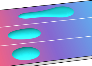
We begin the presentation of our results by demonstrating two distinct behaviours, namely deformation and elongation, observed in a sessile self-rewetting drop placed on a substrate with a temperature gradient.
In the deformation regime, the drop spreads slightly and eventually reaches a pseudo-steady state, such that the wetted length of the drop  $L_w$ (see figure 3c) does not change with time. By contrast, the drop continuously spreads in the elongation regime, leading to a growing
  $L_w$ with time. Figures 3(a), 3(c) and 3(e) show a drop in the deformation regime at
  $M_1=0.8$ and
  $\theta =45^\circ$ with respect to the interface and streamlines, three-dimensional shape and temporal evolution of
  $L_w$. In this case, the drop spreads in the
  $x$ direction and ends up resting on the substrate with slight deformation. The symmetric flows inside the drop are driven by the Marangoni stresses. In particular, we observe that the instantaneous streamlines do not cross the drop interface (figure 3a), suggesting that the interface of the drop stops evolving and reaches an equilibrium state. The equilibrium state can also be confirmed from the temporal evolution of the wetted length of the drop
  $L_w$ in figure 3(e). It can be seen that the value of
  $L_w$ becomes constant after the initial spreading stage. It is noteworthy that such a state is not stable, and in the presence of small asymmetry, e.g. due to discretization errors, the drop tends to move towards one end. This kind of drop migration is particularly more obvious when the initial position of the drop centre does not precisely coincide with the location with minimum surface tension (i.e.
  $x=0$), which is discussed in further detail in § 3.4.

Figure 3. Illustration of different behaviours (deformation for  $M_1=0.8$ and elongation for
  $M_1=1.0$) of a self-rewetting drop placed at
  $x_{mi}=0$ with
  $\theta =45^\circ$. The interface and contour of streamlines at
  $y=0$ when the droplet exhibits (a) deformation and (b) elongation behaviours. In each panel, the blue dashed line shows the initial interface and the red line represents the interface at a later time. (c,d) The three-dimensional shapes of the drop interface at
  $t=1.0$ and 0.6 in (a,b), respectively. Temporal evolution of the wetted length (
 $L_w$) of the drop exhibiting (e) deformation and (f) elongation behaviours.
Figures 3(b), 3(d) and 3(f) demonstrate the dynamics of the sessile drop in the elongation regime at  $M_1=1.0$ and
  $\theta =45^\circ$. In this case, because of the increase in surface tension in the positive and negative
  $x$ directions, the drop experiences a continuous symmetric spreading about its initial centre (
 $x=0$) (see figure 1b). In fact, the elongation of the drop continues due to the positive feedback from the variation in surface tension (i.e. the longer the drop along the direction of
  $x$, the greater the variation in surface tension it encounters). In this case, the streamlines (figure 3b) always cross the interface in the vicinity of the contact line. The streamlines are symmetric about the
  $y$–
$y$– $z$ plane at
  $x = 0$ due to the initially symmetric geometry of the droplet with its centre at
  $x = 0$. Figure 3(f) shows that
  $L_w$ increases as time progresses indicating that the spreading becomes faster and faster with time. It can be reasonably anticipated that the drop would break up sooner or later.
The behaviours of a self-wetting sessile drop also depend on  $\theta$ for a given set of other parameters. Figure 4 shows the phase diagram of the deformation and elongation behaviours of the drop in
  $M_1$ and
  $\theta$ space. It can be seen that the larger the contact angle of the drop, the higher the surface tension gradient for the elongation behaviour to exhibit. This can be easily understood as increasing the value of
  $\theta$ decreases the horizontal component of the Marangoni stresses. As a result, a large variation of the surface tension is needed to elongate the drop with a relatively large contact angle. In order to predict the boundary separating the deformation and elongation regimes, it is necessary to analyse the force exerted on the drop, which is performed in the next section.

Figure 4. Phase diagram showing the deformation and elongation regimes in terms of  $M_1$ verses
  $\theta$ (in degrees). The values of
  $(M_1, \theta )$ exhibiting the regimes of drop deformation and elongation are designated by triangles and squares, respectively. The theoretical prediction of the boundary separating the two regimes is demonstrated by black solid line, and details can be found in § 3.3.
3.2. Forces exerted on the drop: theoretical modelling
We investigate the mechanism that causes the deformation and elongation of the sessile drop by examining the forces acting on it at the onset of regime transition. It is reasonable to assume that the drop deforms symmetrically about the planes  $AOC$ and
  $BOC$ (figure 5a) because of the symmetric initial and boundary conditions of the droplet interface, temperature and velocity fields. Thus, we analyse the force balance by considering only a quarter of the drop. The forces acting on the drop in the
  $x$ direction are the surface tension force in the
  $y$–
$y$– $z$ symmetric plane (
 $F_{s1}$), the pressure contribution (
 $F_p$) on
  $S_{BOC}$ in the
  $y$–
$y$– $z$ symmetric plane and on the curved surface
  $S_{ABC}$ and the capillary (at the contact line,
  $F_{s2}$) and viscous (
 $F_\mu$) forces exerted by the substrate, wherein
  $A$,
$A$,  $B$,
$B$,  $C$ and
  $O$ denote the points on the quarter drop (figure 5a). Here, the inertial force can be neglected as the flow inside the drop induced by the Marangoni stresses (
 $Re=1$) is close to the Stokes flow regime.

Figure 5. (a) Different forces acting on a quarter of the drop in the positive quadrant. The drop encounters the surface tension force  $(F_{s1})$ from the
  $y$–
$y$– $z$ symmetric plane, the force due to the contact line
  $(F_{s2})$, the capillary pressure
  $(F_p)$ at the
  $y$–
$y$– $z$ symmetric plane and the viscous force
  $(F_\mu )$ from the substrate. We choose the slice between the dashed line and plane
  $AOC$ as the control volume to analyse the viscous stress at the centreline
  $OA$. (b) The micro control volume for the analysis of viscous stress near the contact line. The thick line represents the contact line. (c) A geometric sketch of a slice of the drop at the symmetric plane
  $AOC$ of length
  $L$ and height
  $H$. Here,
  $r_x$ denotes the radius of curvature of the arc
  $\widehat {AC}$. (d) The micro control volume at the interface for the analysis of stress boundary conditions.
Clearly, the geometry information of the drop is essential for evaluating these forces. In the following analysis, only relatively small contact angles are considered, and thus the drop shape is represented by a function  $h(x,y)$. We make two assumptions regarding the shape of the deformed drop:
(i) The arcs
 $\widehat {AC}$ and $\widehat {BC}$ are circular due to the relatively small surface tension variation across the interface. Thus, the arcs $\widehat {AC}$ and $\widehat {BC}$ can be expressed in terms of their radius of curvature, denoted by $r_x$ and $r_y$, respectively:
(3.1)and\begin{equation} h(x,0)=\sqrt{r_x^2-x^2}{-}r_x{+}H\end{equation}(3.2)where\begin{equation} h(0,y)=\sqrt{r_y^2-y^2}{-}r_y{+}H,\end{equation}$H$ is the height of the drop (figure 5c).
$\widehat {AC}$ and $\widehat {BC}$ are circular due to the relatively small surface tension variation across the interface. Thus, the arcs $\widehat {AC}$ and $\widehat {BC}$ can be expressed in terms of their radius of curvature, denoted by $r_x$ and $r_y$, respectively:
(3.1)and\begin{equation} h(x,0)=\sqrt{r_x^2-x^2}{-}r_x{+}H\end{equation}(3.2)where\begin{equation} h(0,y)=\sqrt{r_y^2-y^2}{-}r_y{+}H,\end{equation}$H$ is the height of the drop (figure 5c).(ii) The intersection of the interface and the
$x$–$y$ plane is always an ellipse. Mathematically, the ellipse at $z=h$ can be expressed as
(3.3)where the major diameter\begin{equation} \left (\frac{x}{x_0(h)} \right)^2+\left (\frac{y}{y_0(h)} \right)^2=1,\end{equation}$x_0=\sqrt {r_x^2-(h+H-r_x)^2}$ and the minor diameter $y_0=\sqrt {r_y^2-(h+H-r_y)^2}$ can be derived from (3.1) and (3.2), respectively.


With these assumptions and taking  $y_0|_{h=0}=r_y \sin \theta$ into account, it is straightforward to obtain
 \begin{equation} r_x= \frac{L^2+H^2}{2H} \quad \textrm{and}\quad r_y= \frac{H}{1-\cos\theta}, \end{equation}
where  $L=x_0|_{h=0}$ is the half-wetted length of the drop. Accordingly, the volume of the drop at any instant can be calculated as
 \begin{equation} V=\int_0^H ({\rm \pi} x_0 y_0)\,\textrm{d} z.\end{equation}
Therefore, the geometry of the drop can be described by  $H$,
$H$,  $L$ and
  $\theta$. For a drop with volume
  $V_0$ and
  $\theta$, it would enter the regime of drop deformation if a force balance could be reached. In such cases, the geometric parameters
  $H$ and
  $L$ can be uniquely determined, along with the volume constraint (3.5).
In order to justify our assumptions of the drop geometry in the deformation regime, the drop shapes and the curvature at the top of the drop in the  $x$–
$x$– $z$ and
  $y$–
$y$– $z$ planes obtained theoretically and from our numerical simulations are compared in figure 6 for different values of
  $\theta$ and
  $M_1$. It can be seen that good agreements have been achieved.

Figure 6. Comparison of the numerically and theoretically obtained curvature at the top point of the interface and drop shapes in the (a)  $x$–
$x$– $z$ and (b)
  $y$–
$y$– $z$ planes. Four sets of parameters are considered:
  $\theta =15^\circ$ and
  $M_1=0.1$;
  $\theta =30^\circ$ and
  $M_1=0.3$;
  $\theta =45^\circ$ and
  $M_1=0.8$; and
  $\theta =60^\circ$ and
  $M_1=1.2$. Numerically and theoretically obtained drop shapes are represented by solid and dashed lines, respectively.
Thus, with the geometrical information of the drop, the forces acting on it can be estimated. The pressure contribution  $F_p$ can be expressed as
  $\int _{S_{BOC}} (p-p_\infty )\,\textrm {d} S$ by projecting the curved surface onto the
  $y$–
$y$– $z$ plane, where the pressure outside the drop
  $p_\infty$ is assumed to be uniform, i.e. the ambient pressure, and the drop pressure
  $p$ on the
  $BOC$ plane is assumed to be constant due to the weak flow in the symmetric plane
  ${BOC}$. As a result, we can obtain the approximation of
  $p-p_\infty =\gamma |_{x=0}\ (1/r_x+1/r_y)$. Here
  $F_{s1}$ and
  $F_{s2}$ can be expressed as
  $F_{s1} =\int _{\widehat {BC}} \gamma \,\textrm {d} l$ and
  $F_{s2}=\int _{\widehat {AB}}\gamma \cos \theta \sin \alpha \,\textrm {d} l$, respectively, where
  $\alpha$ is the angle at which the tangent at the contact line intersects with the
  $x$ axis as shown in figure 5(b). Furthermore, the heat transfer inside the drop is mainly dominated by the thermal conduction, because of small
  $Ma$ (
 $=0.7$) and small aspect ratio
  $(H/L)$ of the drop. It is reasonably expected that the temperature distribution in the drop is uniform in the vertical direction, i.e.
  $T(x,y,z)=T(x,y,0)$, and thus the surface tension coefficient
  $\gamma$ can be calculated by substituting the corresponding substrate temperature into (2.11). For a given value of
  $\gamma$ and drop geometry,
  $F_p$,
  $F_{s1}$ and
  $F_{s2}$ can be obtained analytically as
 \begin{gather} F_{s1}=r_y \theta\left(1-\frac{M_1}{2} \right), \end{gather}
 \begin{gather}F_{s2}=\left(1-\frac{M_1}{2}+\frac{M_1L^2}{27} \right)r_y\sin\theta \cos\theta, \end{gather}
 \begin{gather}F_p=\left(1-\frac{M_1}{2} \right) \left(\frac{1}{r_x}+\frac{1}{r_y} \right)\left(\frac{r_y^2\theta}{2}-\frac{r_y (r_y-H)\sin\theta}{2}\right). \end{gather}
 The calculation of the viscous force  $F_\mu$ is more complicated than that of the other forces, owing to the complex velocity field inside the drop. If the viscous stress at the centreline
  $\tau _{OA}$ (figure 5a) and contact line
  $\tau _{CL}$ (figure 5b) can be estimated, the variation of the viscous stress at the wetted area can be approximated accordingly. Therefore, we establish a local cylindrical coordinate system
  $(s,r,\varphi )$ at the contact line to analyse the local viscous stress, with
  $s$ and
  $r$ denoting the directions parallel to and normal to the contact line, respectively, and
  $\varphi$ the angle between the
  $r$ axis and the substrate (figure 5b). As the term
  $\partial /\partial s$ vanishes for
  $r\rightarrow 0$ and the flows in the vicinity of the contact line are essentially in the Stokes flow regime, the three-dimensional momentum equation (2.8) can be simplified into two-dimensional equations:
 \begin{gather} \frac{1}{r}\frac{\partial}{\partial r}\left(r\frac{\partial u_s}{\partial r}\right)+ \frac{1}{r^2}\frac{\partial^2 u_s}{\partial \varphi^2}=0, \end{gather}
 \begin{gather}\frac{\partial p}{\partial r}+\frac{1}{r}\frac{\partial}{\partial r}\left(r\frac{\partial u_r}{\partial r}\right)+\frac{1}{r^2}\frac{\partial^2 u_r}{\partial \varphi^2}-\frac{u_r}{r^2}-\frac{2}{r^2}\frac{\partial u_\varphi}{\partial \varphi}=0, \end{gather}
 \begin{gather}\frac{1}{r}\frac{\partial p}{\partial \varphi}+\frac{1}{r}\frac{\partial}{\partial r}\left(r\frac{\partial u_\varphi}{\partial r}\right)+\frac{1}{r^2}\frac{\partial^2 u_\varphi}{\partial \varphi^2}-\frac{u_\varphi}{r^2}+\frac{2}{r^2}\frac{\partial u_r}{\partial \varphi}=0, \end{gather}
where  $u_s$,
  $u_r$ and
  $u_\varphi$ are the velocity components in the
  $s$,
$s$,  $r$ and
  $\varphi$ directions, respectively. Accordingly, the viscous stress of the substrate near the contact line can be expressed as
 \begin{equation} \tau_{r \varphi}|_{\varphi=0}=\frac{1}{r} \left( \frac{\partial u_s}{\partial \varphi}{{\bf e}_s}+ \frac{\partial u_r}{\partial \varphi}{{\bf e}_r} \right), \end{equation}
where  ${{\bf e}_s}$ and
  ${{\bf e}_r}$ are the unit vectors in the
  $s$ and
  $r$ directions, respectively.
We assume that the solution of the velocity component in the  $s$ direction takes the form
  $u_s=f(\varphi )r^n$, where
  $f(\varphi )$ is an undetermined function. Its boundary conditions at the interface and substrate yield
 \begin{equation} u_s|_{\varphi=0}=0\quad \text{and}\quad \frac{1}{r}\left.\frac{\partial u_s}{\partial \varphi}\right|_{\varphi=\theta}= \frac{\gamma_T T_x}{Ca \cos\alpha}, \end{equation}
where  $\gamma _T={\partial \gamma }/{\partial T}$. Substituting
  $u_s=f(\varphi )r^n$ in (3.9), we get
 \begin{equation} n^2f(\varphi)+f''(\varphi)=0, \end{equation}
and the boundary conditions (3.13a,b) can be rewritten as
 \begin{equation} f(0)=0 \quad \text{and}\quad f'(\theta)=\frac{\gamma_T T_x}{Ca \cos\alpha r^{n-1}}. \end{equation}
It is easy to deduce that  $n=1$ in (3.15a,b) as
  $f(\varphi )$ is not a function of
  $r$. Now, integrating (3.14), we get
 \begin{equation} u_s=\frac{r\gamma_TT_x\sin\varphi}{Ca \cos\theta\cos\alpha}. \end{equation}
To solve the velocity components  $u_r$ and
  $u_\varphi$, we use the stream function
  $\varPsi$ and vorticity
  $\omega$ to represent the Navier–Stokes and continuity equations (also, note that
  $\partial u_s/\partial s=0$) (Huh & Scriven Reference Huh and Scriven1971) as
 \begin{equation} u_r=\frac{1}{r}\frac{\partial \varPsi}{\partial \varphi} \quad \text{and}\quad u_\varphi=\frac{\partial \varPsi}{\partial r}. \end{equation}
Taking the curl of (3.10) and (3.11) and given that  $\omega =\nabla _{r \varphi }\times {\bf u}=\nabla ^2_{r \varphi } \varPsi$, a two-dimensional biharmonic equation of
  $\varPsi$ can be obtained as
 \begin{equation} \nabla^4_{r \varphi} \varPsi=0. \end{equation}
The boundary conditions for  $\varPsi$ are the following.
(i) No penetration at the interface:
(3.19)\begin{equation} u_\varphi |_{\varphi=\theta}=\left.\frac{\partial \varPsi}{\partial r}\right|_{\varphi=\theta}=0. \end{equation}(ii) No-slip condition at the substrate:
(3.20a,b)\begin{equation} u_r |_{\varphi=0}=\frac{1}{r} \left.\frac{\partial \varPsi}{\partial \varphi}\right|_{\varphi=0}=0 \quad \text{and}\quad u_\varphi |_{\varphi=0}=\left.\frac{\partial \varPsi}{\partial r}\right|_{\varphi=0}=0. \end{equation}(iii) The balance of shear stress arising from the Marangoni effect at the interface:
(3.21)where\begin{equation} \tau_{r \varphi} |_{\varphi=\theta}=\frac{1}{r^2} \left.\frac{\partial^2 \varPsi}{\partial \varphi^2}\right|_{\varphi=\theta}={\rm \Delta}\tau_r, \end{equation}${\rm \Delta} \tau _r={\gamma _TT_r}/{Ca}$.


It can be assumed that the solution of  $\varPsi$ has a form of
  $\varPsi =g(\varphi )r^2$, which ensures consistency with the boundary condition (iii). Substituting
  $\varPsi =g(\varphi )r^2$ into (3.18), we get
 \begin{equation} g^{(4)}(\varphi)+4g''(\varphi)=0. \end{equation}
The general solution of  $g(\varphi )$ can be expressed as
  $g(\varphi )=a+b\varphi +c \sin (2\varphi )+d\cos (2\varphi )$, where
  $a$,
$a$,  $b$,
$b$,  $c$ and
  $d$ are unknowns which are determined by solving the following set of equations:
 \begin{equation} \begin{bmatrix} 1 & 0 & 0 & 1 \\ 1 & t & \sin(2 \theta) & \cos(2 \theta)\\ 0 & 1 & 2 & 0\\ 0 & 0 & -4\sin(2 \theta) & -4\cos(2 \theta) \end{bmatrix} \begin{bmatrix} a\\b\\c\\ d \end{bmatrix}=\begin{bmatrix} 0\\0\\0\\ {\rm \Delta}\tau_r \end{bmatrix}. \end{equation}
 Thus, we can obtain the solution of  $u_r$ near the contact line as
 \begin{equation} \frac{1}{r}\left.\frac{\partial u_r}{\partial \varphi}\right|_{\varphi=0}=g''(0)={-} \frac{{\rm \Delta}\tau_r(\sin(2\theta)-2\theta)}{(\sin(2\theta)-2\theta\cos(2\theta))}. \end{equation}
Substituting (3.16) and (3.24) into (3.12), we get the expression of viscous stress near the contact line. Accordingly, the viscous stress exerted by the substrate on the drop at the contact line in the  $x$ direction is given by
 \begin{equation} \tau_{zx}|_{CL}={-}\frac{\gamma_TT_x \cos^2\alpha}{\cos\theta}+ \gamma_TT_x \sin^2\alpha\frac{(2\theta-\sin(2\theta))}{(\sin(2\theta)-2\theta\cos(2\theta))}. \end{equation}
 The theoretical prediction of the viscous stress  $\tau _{zx}$ at the contact line obtained from (3.25) is compared with that obtained from the numerical simulation in figure 7(a) for
  $\theta =30^\circ$ and
  $M_1= 0.4$. It can be seen that theoretical prediction and numerical simulation are similar, with respect to the trends in the variation of
  $\tau _{zx}|_{CL}$ versus
  $x$.
$x$.

Figure 7. Comparison of the viscous stress  $\tau _{zx}$ obtained from theoretical prediction and numerical simulation. (a) At the contact line for
  $(\theta , M_1) = (30^\circ , 0.4)$ and (b) at the centreline
  $OA$ for different values of the contact angle
  $\theta$ and
  $M_1$, specifically
  $\theta =45^\circ$ and
  $M_1=$0.8,
  $\theta =30^\circ$ and
  $M_1=0.4$,
  $\theta =15^\circ$ and
  $M_1=0.1$.
Next, we analyse the viscous stress exerted by the substrate close to the line  $OA$ by choosing a thin slice containing the symmetry plane
  $AOC$ as the control volume (figure 5c). The lubrication approximation (Karapetsas et al. Reference Karapetsas, Sahu, Sefiane and Matar2014) is adopted to model the flows inside the control volume, thereby reducing the momentum equation in the
  $x$ direction to
 \begin{equation} Ca \frac{\partial ^2 u}{\partial z^2}= \frac{\partial p}{\partial x}. \end{equation}
The interfacial stress balance condition can be written as  $\tau _{zx}|_{z=h}= -\gamma _T T_x \cos \theta _1-(p-p_\infty ) \tan \theta _1$, where
  $\theta _1$ is the local angle between the interface and the
  $x$ axis. As the contact angle is small, we can assume
  $\theta _1\ll 1$, and thus the interfacial stress balance condition can be simplified as
 \begin{equation} \tau_{zx}|_{z=h}={-}\gamma_T T_x. \end{equation}
Also, we can assume that the temperature inside the drop  $T(x,y,z)$ is independent of
  $z$ and equal to the temperature of the substrate for small values of the contact angle, i.e.
  $T(x,y,z)=T_s(x,y,0)$. Taking account of the symmetry condition at the centreline
  $OA$, we get
  $\tau _{zx}|_{z=h}= -Ca ({\partial u}/{\partial z}) (x,0,h)$ by definition. Substituting this into (3.27), we obtain the boundary condition for the velocity component
  $u$ at the interface:
 \begin{equation} \frac{\partial u}{\partial z}(x,0,h)=\frac{1}{Ca} \gamma_T T_x. \end{equation}
The no-slip condition is imposed at the substrate  $(z=0)$ such that
 \begin{equation} u(x,0,0)=0. \end{equation}
Integrating (3.26) and using the two boundary conditions discussed above, we can obtain the solution of  $u$ under the lubrication approximation in the symmetry plane
  $AOC$ as
 \begin{equation} u(x,0,z)=\frac{1}{Ca} \left[ \frac{h^2}{2}\frac{\partial p}{\partial x} \left(\frac{z^2}{h^2}-\frac{2z}{h}\right)+ \gamma_T T_x z\right].\end{equation}
 On the other hand, the drop in the deformation regime is supposed to experience a pseudo-steady state. In other words, there is no net flux across any vertical plane, i.e.  $\int ^h_0 u\,\textrm {d} z=0$. Substituting (3.30) into this constraint, we obtain
 \begin{equation} \frac{\partial p}{\partial x}=\frac{3\gamma_T T_x}{2h}. \end{equation}
Therefore, the shear stress  $\tau _{zx}$ at the centreline
  $OA$, denoted by
  $\tau _{OA}$, can be obtained as
 \begin{equation} \tau_{OA}={-}Ca \frac{\partial u}{\partial z}=\frac{\gamma_T T_x}{2}. \end{equation}
 The theoretical predictions of the shear stress at the centreline  $OA$ and the corresponding numerical results obtained for different values of
  $M_1$ and
  $\theta$ are presented in figure 7(b). It can be seen that theoretical predictions generally agree well with the numerical results for
  $\theta \le 45^\circ$, especially in the region away from the contact line. The theoretical predictions for larger contact angles are not reliable, because in principle the lubrication approximation is only valid for small contact angles.
Given the theoretical prediction of  $\tau _{zx}$ at the contact line and the symmetry boundary
  $OA$, we approximate the distribution of shear stress in the
  $y$ direction in the wetted area by the following interpolation:
 \begin{equation} \tau_{zx}=\tau_{OA}+(\tau_{CL}-\tau_{OA})\frac{y^n}{W(x)^n}, \end{equation}
where  $W(x)=({H\sin \theta }/{(1-\cos \theta )})\sqrt {1-{x^2}/{L^2}}$ is a half of the wetted width and
  $n$ is a fitting parameter. Figure 8(a) shows the variation of
  $\tau _{zx}$ for different values of
  $n$. Clearly,
  $n=1$ corresponds to a linear interpolation in the
  $y$ direction, while
  $n \to \infty$ is equivalent to setting
  $\tau _{zx} = \tau _{OA}$ as adopted by Pratap et al. (Reference Pratap, Moumen and Subramanian2008). Figure 8(b) shows a comparison of
  $\tau _{zx}$ obtained using (3.33) with
  $n=4$ and the numerical result for
  $\theta \le 30^\circ$ and
  $M_1=0.4$ at
  $x=-0.2$,
  $-0.5$ and
  $-0.8$. Thus, it can be concluded that (3.33) can predict the distribution of
  $\tau _{zx}$ along the
  $y$ direction on the substrate quite satisfactorily. Therefore, we use (3.33) with
  $n=4$ to approximate the shear stress exerted at the wetted area in the following sections.

Figure 8. (a) Typical variations of the viscous stress profiles for  $n=1$, 2, 4, 8 and 16. (b) Comparison of the distribution of the viscous stress
  $\tau _{zx}$ between theory (lines) and numerical result (symbols) at
  $x= -0.2$ (red dashed line with square symbols),
  $-0.5$ (black solid line with circle symbols) and
  $-0.8$ (blue dash-dotted line with triangle symbols) for
  $\theta =30^\circ$ and
  $M_1=0.4$. The top-right inset shows the contour of the viscous stress
  $\tau _{zx}$ at the half-wetted area of the substrate, wherein the vertical lines represent the three typical positions chosen to demonstrate the
  $\tau _{zx}$ profiles.
3.3. Critical conditions for regime transition
For a given drop volume  $V_0$, the drop geometry can be described by
  $L$ and
  $\theta$. Such a shape would represent the drop at equilibrium if the force balance could be reached, i.e. the net force acting on the drop,
  $F_e=F_{s1}+F_{s2}+F_{p}+F_{\mu }=0$. Otherwise, the drop would be elongated when
  $F_e>0$ or become shorter when
  $F_e<0$. Fortunately, all the forces can be theoretically predicted as discussed in § 3.2 for a known drop geometry. Accordingly, we can determine whether the drop reaches the equilibrium state (i.e. falling into the regime of drop deformation) by analysing the variation of the net force with drop deformation.
Figure 9 shows the theoretical prediction of  $F_e$ as a function of
  $L$ at
  $\theta =30^\circ$ for different values of
  $M_1$. It can be seen that with an increase of
  $L$,
$L$,  $F_e$ decreases first and then increases for all values of
  $M_1$. For a relatively small value of
  $M_1$, e.g.
  $M_1=0.4$, the drop tends to spread initially with
  $F_e>0$. Then, it is supposed to reach an equilibrium state in the regime of drop deformation, at which
  $F_e$ becomes zero and the corresponding drop length
  $L_{eq} \approx 1.15$. Note that this state is very stable, because the drop will go back to this point even if
  $L$ happens to be larger than
  $L_{eq}$. We also find that the theoretical prediction of
  $L_{eq}$ is rather close to the numerical results under the same conditions (
 $L_{eq}=1.17$), which justifies the theoretical analysis. On the other hand, for a relatively large value of
  $M_1$, e.g.
  $M_1=0.6$,
  $F_e$ is found to be always greater than zero, implying that the drop would not stop spreading until it breaks up. Therefore, it is reasonable to expect that the drop would fall into the elongation regime, and it does in the numerical simulations. Under certain conditions (
 $M_1 =0.51$ and
  $\theta =30^\circ$ here), the equilibrium state corresponds to the lowest point of the
  $F_e$–
 $L$ curve. In this case, it represents the critical condition of regime transition between drop deformation and drop elongation.

Figure 9. The variations of the theoretically obtained dimensionless net external force  $F_e$ as a function of
  $L$ at
  $\theta =30^\circ$ for different values of
  $M_1$. The grey dashed line indicates
  $F_e=0$, i.e. all the forces are balanced. Here
  $F_e<0$ and
  $F_e>0$ denote the drop retracting and spreading regions, respectively.
Thus, the critical condition of regime transition can be determined by
 \begin{equation} \min(F_e (L ,\theta,M_1)|_{L \in(0,\infty)})=0.\end{equation}
We can predict the boundary separating the deformation and elongation regimes based on (3.34), and the obtained result is superimposed onto the numerical data in figure 4. It is clear that the theoretical prediction agrees well with the numerical results.
3.4. Drop migration and spreading
So far we have discussed the conditions associated with the deformation and elongation regimes for  $x_{mi}=0$, i.e. when the initial location of the centre of the drop coincides with the location associated with the minimum surface tension
  $(x=0)$. In this section, we investigate the dynamics when the drop is initially placed slightly away from
  $x=0$. When
  $x_{mi} \ne 0$, the drop experiences an asymmetric surface tension distribution along the
  $x$ direction. Figures 10(a,c) and 10(b,d) depict the drop dynamics for initial placement at
  $x_{mi}=0.1$ with
  $\theta =30^\circ$ for
  $M_1=0.3$ and 0.6, respectively. Figure 10(a,c) corresponds to the deformation regime for
  $M_1=0.3$. It can be seen that the shape of the drop almost remains a spherical cap, but it migrates significantly in the
  $x$ direction. In contrast, the drop dynamics depicted in figure 10(b,d) for
  $M_1=0.6$ is markedly different. In this case, the drop exhibits an elongation behaviour. It can be seen in figure 10(b,d) that the drop deforms significantly and spreads much faster than that observed for
  $M_1=0.3$ (figure 10a,c). The drop for
  $M_1=0.6$ also migrates in the positive
  $x$ direction due to the asymmetric surface tension distribution (resulting in unbalanced Marangoni stresses) because of the initial location of the drop (
 $x_{mi} \ne 0$). This elongation behaviour of the drop (in figure 10b,d) is different from that observed in figure 3(b) for
  $x_{mi}=0$.

Figure 10. Temporal evolutions of (a,b) the drop and (c,d) the wetted area when the initial location is  $x_{mi}=0.1$ and the value of the contact angle is
  $\theta =30^\circ$: (a,c)
  $M_1=0.3$ and (b,d)
  $M_1=0.6$. In (c,d), the shapes of the wetted area of the drop are shown at time intervals of
  $0.2$ starting from
  $t=0.1$.
Figure 11(a) depicts the variations of the  $x$ coordinate of the centre of mass of the drop
  $x_m$ with
  $t$ for different values of
  $M_1$. Here, a logarithmic coordinate of
  $t$ is adopted to facilitate easy comparison between the results for different values of
  $M_1$. It can be seen that the larger the value of
  $M_1$, the faster the drop spreads, due to the increase of the surface tension gradient in the
  $x$ direction at
  $x=x_m$, i.e.
  $\partial \gamma /\partial x|_{x=x_m}$. If the height of the drop is small, the temperature can be assumed to be constant in the
  $z$ direction, and thus
  $\partial \gamma /\partial x|_{x=x_m}$ is proportional to
  $M_1x_m$. The variations of
  $M_1 x_m$ with the velocity of the centre of mass of the drop
  $U_m$ (
 $= \partial x_m/\partial t$) for different values of
  $M_1$ are shown in figure 11(b). It can be seen that all the curves collapse to a single line with a slope equal to one, i.e.
  $U_m \varpropto M_1x_m$ at the early stage of drop migration. However, at the later stage, this scaling does not hold good due to the deformation of the drop. A similar conclusion was previously proposed for two-dimensional (Ford & Nadim Reference Ford and Nadim1994; Gomba & Homsy Reference Gomba and Homsy2010) and three-dimensional (Pratap et al. Reference Pratap, Moumen and Subramanian2008) sessile drops of a normal fluid (i.e. when surface tension decreases linearly with temperature). Integrating
  $\partial x_m/ \partial t\varpropto M_1x_m$ and applying the initial condition
  $x_m|_{t=0}=x_{mi}$, we get
  $x_m=x_{mi} \exp ({A\times M_1 t})$, wherein
  $A$ is the fitting constant, whose value lies in the range [5.20, 5.65]. It is interesting to note that this relation also works well even for the case when the drop is placed at the location of the minimum surface tension. For the result presented by the thick grey line in figure 11(b),
  $x_{mi}=3.06\times 10^{-7}$ and
  $A=5.40$, which are obtained by fitting the
  $x_m$–
 $t$ curve with the exponential function. The negligible deviation of
  $x_{mi}$ from zero (which is set in our numerical simulation) is due to the discretization errors. Nevertheless, as the value of the fitting parameter
  $A$ is close to those for the other cases with
  $x_{mi} \neq 0$, it can be concluded that the theory discussed is quite general for predicting the behaviour of drop migration.

Figure 11. Variations of the numerically obtained (a) centre of mass of the drop  $x_m$ with
  $t$ and (b)
  $M_1 x_m$ with the velocity of the centre of mass of the drop
  $(U_m)$ for different values of
  $M_1$ for
  $\theta = 30^\circ$. Here,
  $x_{mi} = 0.1$ for all cases except the results presented by the thick grey dashed line in (b) for which
  $x_{mi}=0$ and
  $M_1=0.4$.
Next, we investigate the spreading behaviour of the drop. Figures 12(a) and 12(b) show the variations of the wetted length of the drop  $L_w$ versus
  $t$ for different values of
  $\theta$ and
  $M_1$ exhibiting deformation and elongation dynamics, respectively. Let us take the case of
  $\theta =30^\circ$ and
  $M_1=0.3$ (solid red line in figure 12a) as an example to explain the behaviour of the drop with
  $x_{mi}=0.1$ in the deformation regime. It can be seen that the drop exhibits three distinct spreading behaviours during the early, intermediate and late stages. At the early stage (
 $t<0.5$ approximately), the drop undergoes spreading due to the self-rewetting nature of the drop liquid. At the intermediate stage (
 $0.5<t<1.0$ approximately), the wetted length of the drop becomes almost constant (i.e. the drop stops spreading) while it migrates aside. At the late stage (
 $t>1.0$ approximately), the drop again spreads and migrates towards one side as the surface tension increases as it moves away from
  $x=0$. Close inspection of figure 12(a) also reveals that the duration of the intermediate stable stage of the drop increases as the value of
  $M_1$ decreases. It can be seen that for
  $M_1=0.2$ and
  $\theta =30^\circ$, the drop almost remains stable (no deformation) for the entire duration. On the other hand, in figure 12(b), the drop continues to elongate all the time. It can be seen that, for a fixed value of
  $\theta$, increasing the surface tension gradient (increasing the value of
  $M_1$) increases the deformation of the drop. To summarize, in figure 12, we demonstrate the deformation and elongation behaviours of the drop for the same initial condition for different values of
  $\theta$ and
  $M_1$ and found that the intermediate region disappears when
  $\theta$ and
  $M_1$ are close to the critical condition.

Figure 12. Variations of the wetted length of the drop  $L_w$ versus
  $t$ for different values of
  $\theta$ and
  $M_1$ in the (a) deformation and (b) elongation regimes. Here,
  $x_{mi}=0.1$.
Finally, we present the variation of the wetted length  $L_w$ of the drop (i.e. spreading behaviour) with the motion of the
  $x$ coordinate of its centre of mass
  $x_m$ (migration behaviour) for different values of
  $x_{mi}$. For this purpose, we choose
  $M_1=0.3$ and 0.6 in figures 13(a) and 13(b), respectively. Interestingly in the deformation regime (
 $M_1=0.3$), it can be observed that the
  $L_w$ versus
  $x_m$ curves for different values of
  $x_{mi}$ collapse to a linear line after the initial spreading stage. On the other hand, in the elongation regime (
 $M_1=0.6$), the spreading rate of the drop at a given location increases as the value of
  $x_{mi}$ decreases (i.e. when the drop starts from a location closer to the location of the minimum surface tension).

Figure 13. Variations of the wetted length  $L_w$ with the
  $x$ coordinate of the centre of mass of the drop
  $x_m$ started from different initial locations on the substrate: (a)
  $M_1=0.3$ and
  $x_{mi}=0.1$, 0.2, 0.4, 0.6, 1.0 and 1.5; (b)
  $M_1=0.6$ and
  $x_{mi}=0.1$, 0.2, 0.4, 0.6. The values of
  $M_1t$ are at the points shown by the black dots. Here,
  $\theta =30^\circ$.
4. Conclusions
The dynamics of sessile drops of self-rewetting liquids whose surface tension exhibits a parabolic dependency with temperature has been investigated via three-dimensional numerical simulations. The substrate is maintained at an isothermal condition with its temperature increasing linearly in the horizontal direction. First, we investigate the drop dynamics when it is placed at the location of the minimum surface tension. In this case, two distinct regimes, where the drop undergoes deformation and elongation behaviours, are observed. In the deformation regime, the drop experiences a short initial spreading stage, and then enters a pseudo-steady stage. On the other hand, in the elongation regime, the drop spreads about its initial location due to the increase in the surface tension of the self-rewetting liquid in both positive and negative  $x$ directions. The gradient of surface tension (characterized by
  $M_1$) and the contact angle of the drop
  $(\theta )$ are found to influence these regimes for a fixed set of other parameters. It is observed that the deformation and the elongation regimes are associated with low and high values of
  $M_1$ for a fixed value of
  $\theta$. A phase diagram showing the deformation and the elongation regimes is also plotted in the
  $M_1$–
 $\theta$ plane.
To understand the underlying mechanism of these distinct drop dynamics, we analyse different forces acting on a quarter of the drop, namely the viscous force  $(F_\mu )$, the surface tension force acting at the symmetric plane
  $(F_{s1})$, the force due to the contact line
  $(F_{s2})$ and the capillary pressure force
  $(F_p)$. Forces
  $F_{s1}$,
  $F_{s2}$ and
  $F_{p}$ are obtained using the geometric assumptions which have been validated by our numerical simulations. We derive the theoretical expression of the viscous stresses at the centreline and near the contact line. The theoretically obtained viscous stress exerted by the substrate on the drop is in good agreement with numerical simulation, when a fitted parameter (
 $n=4$) is used. Using these viscous stresses, the viscous force
  $(F_\mu )$ acting on the drop is calculated. The critical condition demarcating the deformation and elongation regimes is obtained by balancing the theoretically obtained forces acting on the drop.
In the theoretical calculations, the initial location of the drop coincides with the location of the minimum surface tension of the self-rewetting liquid. Thus, to draw a more general conclusion, we numerically investigate the drop dynamics with its initial location slightly away from the point of the minimum surface tension. The migration and spreading dynamics are studied separately. It is observed that the  $x$ coordinate of the centre of mass of the drop evolves initially as
  $x_m=x_{mi} \exp ({A\times M_1 t})$, where
  $A$ is a fitting parameter related to the contact angle
  $\theta$. At the later stage, the spreading of the drop makes the dynamics more complex and does not obey the initial trend. We also demonstrate the spreading behaviour of the drop with
  $x_{mi} \ne 0$ for the parameters associated with the deformation and elongation regions. It is observed that in the deformation regime, the drop spreads slightly and then experiences a pseudo-steady state, which increases with decreasing value of
  $M_1$ and finally spreads again. For a set of parameters associated with the elongation regime, the drop continues to spread all the time. Finally, we also investigate the dependency of the wetted length of the drop on the location of its centre of mass and observe that while the curves for different values of
  $x_{mi}$ collapse to a single linear curve after the initial spreading stage in the deformation regime, the spreading rate of the drop increases as the value of
  $x_{mi}$ decreases in the elongation regime.
It is to be noted that numerical slip is introduced to remove the stress singularity at moving contact lines. The numerical slip in the diffuse interface model can be measured by the slip length (Ding & Spelt Reference Ding and Spelt2007), and could affect the spreading dynamics of a drop in the elongation regime. Thus, it can be expected that the larger the slip length, the faster the spreading of the drop, and the more significant the Marangoni stresses exerted on the drop. The effect of the slip length on the dynamic behaviour of elongated drops is beyond the scope of the present study but will be a focus of our future research.
Funding
H.D. is grateful for the support of the National Natural Science Foundation of China (grant nos. 11425210, 11621202, 11672288, 11932019), the Strategic Priority Research Program of the Chinese Academy of Sciences (grant no. XDB22040103) and the Fundamental Research Funds for the Central Universities. K.C.S. also thanks the Science and Engineering Research Board, India for providing financial support (grant no. MTR/2017/000029).
Declaration of interests
The authors report no conflict of interest.
Author contributions
Z.-L.X. and J.-Y.C. contributed equally to this article.


