


1 Introduction
Large wind farms with dozens of wind turbines arranged in multiple rows are increasingly built worldwide to reduce the usage of unsustainable fossil fuels. The spacing between the adjacent turbine rows/columns is typically selected as 3–10 times the rotor diameter, due to the limitations of land usage and connection cable length. At such a spacing, the power losses caused by the inevitable wake interactions can reach up to approximately 40 %, when the directions of turbine rows/columns are aligned with the wind direction (Stevens & Meneveau Reference Stevens and Meneveau2017; Porté-Agel, Bastankhah & Shamsoddin Reference Porté-Agel, Bastankhah and Shamsoddin2019). To minimize these power losses, a fast prediction of the wind farm power output in various wind conditions is needed in the layout design phase, which in practice is realized by computationally cheap analytical methods. Specifically, the wake velocity deficits caused by the individual wind turbines are first computed from analytical wake models, and then superimposed to get the total wake deficit (Jensen Reference Jensen1983; Niayifar & Porté-Agel Reference Niayifar and Porté-Agel2016), as sketched in figure 1.

Figure 1. Sketch of wake superposition in a three-row wind farm. Here,  $u_{s}^{i}$ denotes the wake velocity deficit caused by the
  $i$th wind turbine.
Depending on the reference wind speed used to calculate the individual wakes (either local or global) and the operations adopted to combine the wakes (either summing the wake velocity deficits, or summing the squares of the wake velocity deficits), four wake superposition methods are available in the literature (Stevens & Meneveau Reference Stevens and Meneveau2017; Porté-Agel et al. Reference Porté-Agel, Bastankhah and Shamsoddin2019), as follows.
 $$\begin{eqnarray}\displaystyle & \displaystyle \text{Method A}:~U_{w}(x,y,z)=U_{\infty }-\mathop{\sum }_{i}(U_{\infty }-u_{w}^{i}(x,y,z)). & \displaystyle\end{eqnarray}$$
 $$\begin{eqnarray}\displaystyle & \displaystyle \text{Method B}:~U_{w}(x,y,z)=U_{\infty }-\sqrt{\mathop{\sum }_{i}(U_{\infty }-u_{w}^{i}(x,y,z))^{2}}. & \displaystyle\end{eqnarray}$$
 $$\begin{eqnarray}\displaystyle & \displaystyle \text{Method C}:~U_{w}(x,y,z)=U_{\infty }-\mathop{\sum }_{i}(u_{0}^{i}-u_{w}^{i}(x,y,z)). & \displaystyle\end{eqnarray}$$
 $$\begin{eqnarray}\displaystyle & \displaystyle \text{Method D}:~U_{w}(x,y,z)=U_{\infty }-\sqrt{\mathop{\sum }_{i}(u_{0}^{i}-u_{w}^{i}(x,y,z))^{2}}. & \displaystyle\end{eqnarray}$$
 Here,  $u_{0}^{i}$ is the mean wind velocity perceived by the
  $i$th wind turbine (referred to as
  $\text{WT}_{i}$ hereinafter);
  $u_{w}^{i}$ is the wake velocity induced by
  $\text{WT}_{i}$ in stand-alone conditions. The difference between the incoming wind velocity and the wake velocity defines the individual wake velocity deficit, i.e.
  $u_{s}^{i}=u_{0}^{i}-u_{w}^{i}$.
The logic behind each of these methods is briefly explained here. In Method A (Lissaman Reference Lissaman1979), a large wind turbine spacing with weak wake interaction is assumed, such that, during the calculation of individual wakes, the mean wind velocity experienced by the downstream wind turbines can be substituted by the inflow velocity of the wind farm, i.e.  $u_{0}^{i}\approx U_{\infty }$. Further, since the wake velocity deficit is small, the momentum deficit term
  $(U_{\infty }-u_{s}^{i})\cdot u_{s}^{i}$ can be approximated by
  $U_{\infty }\cdot u_{s}^{i}$. Consequently, to conserve the total momentum deficit in the wake (i.e. total wind turbine thrust), one only needs to sum the wake velocity deficits linearly, like a passive scalar. Method B (Katic, Højstrup & Jensen Reference Katic, Højstrup and Jensen1987) makes a similar assumption of
  $u_{0}^{i}\approx U_{\infty }$ during the calculation of individual wakes. Nevertheless, the wake superposition is realized by summing the squares of the wake velocity deficits. By executing this operation, the authors expected to conserve the mean kinetic energy deficit during wake interaction, which is disputable as the mean kinetic energy flux is not conserved in wake flows due to the non-trivial turbulent dissipation.
The counterparts of Methods A and B are Methods C and D proposed by Niayifar & Porté-Agel (Reference Niayifar and Porté-Agel2016) and Voutsinas, Rados & Zervos (Reference Voutsinas, Rados and Zervos1990), respectively. In these two recent methods, similar operations (i.e. linear sum and square sum) are adopted to combine the individual wake velocity deficits without theoretical justification. Nevertheless, during the computation of the individual wakes, the approximation of  $u_{0}^{i}\approx U_{\infty }$ is removed, and the mean wind speeds perceived by the wind turbines
  $u_{0}^{i}$ (
 $i=0,1,2,\ldots$) are determined consecutively from upstream to downstream. Therefore, it is largely expected that Methods C and D will give more accurate predictions of the wind farm power production than their counterparts, particularly in the cases of short wind turbine spacing and large wake velocity deficit.
To summarize, the four existing wake superposition methods are all empirical relations without solid theoretical foundation. During the combination of individual wakes, the total momentum deficit is highly unlikely to be conserved by these methods, which could introduce significant errors in the power prediction of wind farms. In this study, a novel wake superposition method is derived rigorously from the law of conservation of momentum and its superior performance over the other four existing methods is demonstrated by experimental and large-eddy simulation (LES) data.
2 Theoretical derivation
2.1 Linearized expression for the momentum deficit flux
For wake flow, the law of conservation of momentum stipulates that the total momentum deficit flux across the wake cross-section has to be a conserved quantity, equalling the drag imposed to the flow (Pope Reference Pope2000). Applying this principle to each of the wind turbines shown in figure 1, equation (2.1) can be derived (for details, please refer to appendix A),
 $$\begin{eqnarray}T_{i}=\unicode[STIX]{x1D70C}\iint u_{w}^{i}(x,y,z)\cdot u_{s}^{i}(x,y,z)\,\text{d}y\,\text{d}z,\end{eqnarray}$$
 where  $T_{i}$ denotes the thrust of
  $\text{WT}_{i}$. Since the wake velocity
  $u_{w}$ is correlated with the wake velocity deficit, the relationship between
  $T_{i}$ and
  $u_{s}^{i}$ is nonlinear. However, if an appropriate mean wake convection velocity (denoted as
  $u_{c}^{i}$) is selected to represent the spatially dependent wake velocity in the entire wake cross-section, equation (2.1) may be rewritten in the following linear form:
 $$\begin{eqnarray}T_{i}=\unicode[STIX]{x1D70C}\iint u_{c}^{i}(x)\cdot u_{s}^{i}(x,y,z)\,\text{d}y\,\text{d}z=\unicode[STIX]{x1D70C}u_{c}^{i}(x)\iint u_{s}^{i}(x,y,z)\,\text{d}y\,\text{d}z.\end{eqnarray}$$
Substituting (2.2) into (2.1), a mathematical definition of the mean wake convection velocity is given as follows:
 $$\begin{eqnarray}u_{c}^{i}(x)=\frac{\displaystyle \iint u_{w}^{i}(x,y,z)\cdot u_{s}^{i}(x,y,z)\,\text{d}y\,\text{d}z}{\displaystyle \iint u_{s}^{i}(x,y,z)\,\text{d}y\,\text{d}z}.\end{eqnarray}$$
 Namely, the mean convection velocity necessary for linearizing the momentum deficit term is a weighted average of the wake velocity, where the weights are selected as the corresponding wake velocity deficits. Since the analytical expressions for  $u_{w}^{i}$ and
  $u_{s}^{i}$ are widely available in various wind turbine wake models (Jensen Reference Jensen1983; Frandsen et al. Reference Frandsen, Barthelmie, Pryor, Rathmann, Larsen, Højstrup and Thøgersen2006; Bastankhah & Porté-Agel Reference Bastankhah and Porté-Agel2014), the expression for
  $u_{c}^{i}$ can also be derived in different forms. Nevertheless, for the purpose of accurate wind farm power prediction, only the wake models that are derived strictly from the law of conservation of momentum (i.e. excluding the Jensen model) are recommended. Here, the Gaussian wake model proposed by Bastankhah & Porté-Agel (Reference Bastankhah and Porté-Agel2014) is taken as an example. The wake velocity deficit behind the
  $i$th wind turbine reads as
 $$\begin{eqnarray}\frac{u_{s}^{i}}{u_{0}^{i}}=\left(1-\sqrt{1-\frac{C_{t}^{i}}{8\unicode[STIX]{x1D70E}_{y}\unicode[STIX]{x1D70E}_{z}/D^{2}}}\right)\cdot \exp \left(-\frac{y^{2}}{2\unicode[STIX]{x1D70E}_{y}^{2}}-\frac{z^{2}}{2\unicode[STIX]{x1D70E}_{z}^{2}}\right),\end{eqnarray}$$
 where  $D$ is the rotor diameter;
  $C_{t}^{i}$ is the thrust coefficient
  $\text{WT}_{i}$;
  $\unicode[STIX]{x1D70E}_{y}$ and
  $\unicode[STIX]{x1D70E}_{z}$ denote the wake width in the spanwise and vertical directions, respectively. Substituting (2.4) into (2.3), an explicit expression for the mean convection velocity can be obtained:
 $$\begin{eqnarray}\frac{u_{c}^{i}(x)}{u_{0}^{i}}=\frac{1}{2}+\frac{1}{2}\sqrt{1-\frac{C_{t}^{i}}{8\unicode[STIX]{x1D70E}_{y}\unicode[STIX]{x1D70E}_{z}/D^{2}}}.\end{eqnarray}$$
 As a result, the mean wake convection velocity is bounded between  $0.5u_{0}^{i}$ and
  $u_{0}^{i}$, increasing with the wake width and decreasing with the thrust coefficient.
2.2 Momentum-conserving wake superposition principle
To conserve the total momentum deficit (i.e. wind turbine thrust) during wake superposition, the combined wake velocity  $U_{w}$ has to satisfy the following equation:
 $$\begin{eqnarray}\unicode[STIX]{x1D70C}\iint U_{w}(x,y,z)\cdot U_{s}(x,y,z)\,\text{d}y\,\text{d}z=\mathop{\sum }_{i}T_{i}=\mathop{\sum }_{i}\unicode[STIX]{x1D70C}u_{c}^{i}(x)\iint u_{s}^{i}(x,y,z)\,\text{d}y\,\text{d}z,\end{eqnarray}$$
 where  $U_{s}$ is the total wake velocity deficit given by
  $U_{\infty }-U_{w}$. Analogous to (2.3), a mean convection velocity for the combined wake (
 $U_{c}$) can be defined as follows:
 $$\begin{eqnarray}U_{c}(x)=\frac{\displaystyle \iint U_{w}(x,y,z)\cdot U_{s}(x,y,z)\,\text{d}y\,\text{d}z}{\displaystyle \iint U_{s}(x,y,z)\,\text{d}y\,\text{d}z}.\end{eqnarray}$$
Using this relation to simplify (2.6), the following equation is derived:
 $$\begin{eqnarray}\iint U_{s}(x,y,z)\,\text{d}y\,\text{d}z=\mathop{\sum }_{i}\frac{u_{c}^{i}(x)}{U_{c}(x)}\iint u_{s}^{i}(x,y,z)\,\text{d}y\,\text{d}z.\end{eqnarray}$$
At this stage, it becomes evident that, in order to conserve the total momentum during wake superposition, the following expression should be used:
 $$\begin{eqnarray}U_{s}(x,y,z)=\mathop{\sum }_{i}\frac{u_{c}^{i}(x)}{U_{c}(x)}u_{s}^{i}(x,y,z).\end{eqnarray}$$
 Equation (2.9) states that the total wake velocity deficit equals a weighted sum of the individual wake velocity deficits, where the weights are determined by the ratio of  $u_{c}^{i}$ to
  $U_{c}$. This is understandable since, when combining two wakes with the same amount of velocity deficit, the one with the larger convection velocity carries more momentum deficit, and thus should be represented by a higher weight during the velocity deficit addition. In the case of small wake velocity deficits (say,
  $u_{s}^{i}\leqslant 0.1U_{\infty }$),
  $u_{c}^{i}/U_{c}$ may be approximated by 1, and the above expression automatically becomes (1.3) (Method C). However, this only happens when the wind turbine spacing exceeds
  $15D$ (Chamorro & Porté-Agel Reference Chamorro and Porté-Agel2010). Additionally, since the mean convection velocity for the combined wake is unknown prior to wake superposition, an iterative method should be deployed to solve the combined wake velocity out of (2.7) and (2.9). Specifically,
  $U_{c}$ is initialized to be the maximum value of
  $u_{c}^{i}$ and substituted into (2.9) to get an estimated total wake velocity deficit. The estimated total wake velocity deficit is further plugged into (2.7) to get a corrected convection velocity for the combined wake
  $U_{c}^{\ast }$. This iterative correction repeats, until a certain criterion is met (e.g.
  $|U_{c}-U_{c}^{\ast }|/U_{c}^{\ast }\leqslant 0.001$). Typically, no more than five iterations are needed to reach convergence, and the corresponding computation cost is negligible compared to the individual wake computation.

Figure 2. Middle-hub wake velocity contours obtained from: (a) Method A (Lissaman Reference Lissaman1979), (b) Method B (Katic et al. Reference Katic, Højstrup and Jensen1987), (c) Method C (Niayifar & Porté-Agel Reference Niayifar and Porté-Agel2016), (d) Method D (Voutsinas et al. Reference Voutsinas, Rados and Zervos1990), (e) the proposed new method, and (f) particle imaging velocimetry measurements.
3 Model validation
3.1 Particle imaging velocimetry measurements in a three-row wind farm
For validation purposes, the three-row wind farm sketched in figure 1 is constructed in the boundary layer wind tunnel at the WIRE laboratory of EPFL, using the miniature wind turbines designed by Bastankhah & Porté-Agel (Reference Bastankhah and Porté-Agel2017) (WIRE-01, rotor diameter: 0.15 m, hub height: 0.125 m), and the velocity field at the hub-height is measured by a particle imaging velocimetry (PIV) system. The time-averaged wind speed and the turbulence intensity at the hub level are kept at 4.9 m s-1 and 6 %, respectively. The boundary layer thickness, determined by 99 % of the free-stream velocity, is approximately 0.3 m. The streamwise spacing between the wind turbines is fixed at  $5D$, and the optimal rotation speed of each wind turbine is set in situ based on the free rotation speed, following the procedure described in Bastankhah & Porté-Agel (Reference Bastankhah and Porté-Agel2019). The thrust and power coefficients (denoted as
  $C_{t}$ and
  $C_{p}$) of the WIRE-01 turbine at optimal operation are 0.82 and 0.35, respectively (Bastankhah & Porté-Agel Reference Bastankhah and Porté-Agel2016). The PIV system consists of a camera (LaVision-sCMOS), a Litron laser (Nano TRL 425-10) and a programmable timing unit (PTU-v9, LaVision). Both the camera and the laser are mounted on a traversing system, to shift the field of view (FOV) in the streamwise direction. In total, three sets of FOVs are arranged to cover the complete wake evolution in an area of
  $15D\times 5D$. In each FOV, 500 image pairs are recorded to get statistically converged mean velocity fields.
The aforementioned model wind farm is used as a test bench to examine the performance of different wake superposition methods. The individual wake velocity deficits are computed from (2.4) (Bastankhah & Porté-Agel Reference Bastankhah and Porté-Agel2014), and the wake width is modelled as a quasi-linear function of the streamwise coordinate (Shapiro, Gayme & Meneveau Reference Shapiro, Gayme and Meneveau2018):
 $$\begin{eqnarray}\left.\begin{array}{@{}l@{}}\displaystyle \frac{\unicode[STIX]{x1D70E}_{y}}{D}=0.35\cos \unicode[STIX]{x1D6FD}+k_{w}\ln \left[1+\exp \left(\frac{x-x_{th}}{D}\right)\right],\\[13.0pt] \displaystyle \frac{\unicode[STIX]{x1D70E}_{z}}{D}=0.35+k_{w}\ln \left[1+\exp \left(\frac{x-x_{th}}{D}\right)\right],\end{array}\right\}\end{eqnarray}$$
 where  $\unicode[STIX]{x1D6FD}$,
  $k_{w}$ and
  $x_{th}$ denote the yaw angle, the wake spreading rate and the near-wake length, respectively.
Namely, in the near wake, the wake width remains approximately constant, whereas in the far wake, the wake width grows linearly with an asymptotic wake spreading rate of  $k_{w}$. The detailed expression for
  $x_{th}$ is available in Vermeulen (Reference Vermeulen1980). The wake spreading rate is associated with both the ambient turbulence intensity
  $I_{0}$ and the added turbulence intensity
  $I_{+}$, and can be modelled as
  $k_{w}=0.38(I_{0}^{2}+I_{+}^{2})^{1/2}+0.004$, where
  $I_{+}=0.73a^{0.83}I_{0}^{0.03}(x/D)^{-0.32}$ (Niayifar & Porté-Agel Reference Niayifar and Porté-Agel2016). Additionally, to simulate the effect of the near-wake pressure gradient, the thrust coefficients in (2.4)–(2.5) are written as an error function of the streamwise coordinate,
  $C_{t}^{i}(x)=0.82(1+\text{erf}(x/D))/2$, to create a gradual increase of the wake deficit at
  $x<2D$ (Shapiro et al. Reference Shapiro, Gayme and Meneveau2018).
Figure 2 shows the middle-hub velocity fields computed with analytical methods and measured by PIV. As a result of the low ambient turbulence intensity, the near-wake region of  $\text{WT}_{1}$ extends to more than
  $3D$ (figure 2f). In the centreline of this near-wake region, a rather low wake velocity is noticed, which is related to the hub drag. The performance of different wake superposition methods can be appreciated by comparing the wake velocity contours behind
  $\text{WT}_{2}$ and
  $\text{WT}_{3}$, where, due to the increase of turbulence intensity, a short near wake and a fast wake recovery are expected. Methods A and B from Lissaman (Reference Lissaman1979) and Katic et al. (Reference Katic, Højstrup and Jensen1987) fail to reproduce these two phenomena, since the interactions between wind turbines are neglected during the calculation of individual wakes. Method D (Voutsinas et al. Reference Voutsinas, Rados and Zervos1990) delivers a reasonable trend of the near-wake length, whereas the wake velocity deficit is largely underestimated, compared to the experimental data. Consequently, Method C (Niayifar & Porté-Agel Reference Niayifar and Porté-Agel2016) and the proposed new method are the only two methods capable of delivering a satisfactory wind farm wake flow.

Figure 3. Streamwise variations of (a) the centreline wake deficit, (b) the normalized total momentum deficit. Methods A–D are abbreviated as MA–MD in the legends.
Quantitative comparison of the centreline wake velocity (i.e.  $U_{w}|_{y=0}$) is made in figure 3(a). As shown, the centreline wake velocity deficit is largely overestimated by Methods A and B, since both of them fail to account for the fact that the local wind speeds perceived by the downstream wind turbines are always lower than the inflow velocity. Method D, on the contrary, underestimates the centreline wake velocity deficit, which is consistent with the observation in Niayifar & Porté-Agel (Reference Niayifar and Porté-Agel2016). Method C and the proposed new method outperform the other methods by delivering a satisfactory prediction of the centreline wake velocity deficit in the range
  $7\leqslant x/D\leqslant 10$. Nevertheless, the difference in their performance starts to stand out at
  $x/D\leqslant 13$, where the wake velocity predicted by Method C is always 5 % lower than that obtained from the experiment and the new method. This 5 % discrepancy, although still acceptable in the current context, can accumulate to large errors when more turbine rows are added, as will be demonstrated in § 3.2.
Based on the models results shown in figure 2, the normalized total momentum deficit ( $\overline{M}_{d}$) is computed by the following equation:
 $$\begin{eqnarray}\overline{M}_{d}=\frac{\displaystyle 8\iint U_{w}\cdot (U_{\infty }-U_{w})\,\text{d}y\,\text{d}z}{U_{\infty }^{2}\unicode[STIX]{x03C0}D^{2}},\end{eqnarray}$$
where the initial momentum flux across the rotor disk is selected for normalization, analogous to the definition of the wind turbine thrust coefficient.
Theoretically, the total momentum deficit should exhibit a stair-step increase along the streamwise direction, with each step corresponding to the additional thrust/drag induced by a new turbine row. Therefore, to validate the model predictions of  $\overline{M}_{d}$, experimental values of the turbine thrust are required. In the present study, force measurements are not performed, and the power measurement data available in Bastankhah & Porté-Agel (Reference Bastankhah and Porté-Agel2019) are used to estimate the turbine thrust. Specifically, based on the definitions of
  $C_{t}$ and
  $C_{p}$ (0.82 and 0.35 respectively for the WIRE-01 turbine at optimal operation), we have the following two equations:
 $$\begin{eqnarray}\left.\begin{array}{@{}l@{}}\displaystyle P_{i}=C_{p}\cdot \frac{\unicode[STIX]{x1D70C}(u_{0}^{i})^{3}}{2}\cdot \frac{\unicode[STIX]{x03C0}D^{2}}{4},\\[10.0pt] \displaystyle T_{i}=C_{t}\cdot \frac{\unicode[STIX]{x1D70C}(u_{0}^{i})^{2}}{2}\cdot \frac{\unicode[STIX]{x03C0}D^{2}}{4},\end{array}\right\}\end{eqnarray}$$
 where  $P_{i}$ denotes the power production of the
  $i$th turbine (
 $i=1,2,3$). Working out the mean wind speed from the first equation and substituting into the second one, the relation between
  $T_{i}$ and
  $P_{i}$ can be derived:
 $$\begin{eqnarray}T_{i}=C_{t}\cdot \left(\frac{\unicode[STIX]{x1D70C}\unicode[STIX]{x03C0}D^{2}}{8}\right)^{1/3}\cdot \left(\frac{P_{i}}{C_{p}}\right)^{2/3}.\end{eqnarray}$$
 Figure 3 compares the normalized total momentum deficits computed with the analytical models and derived directly from the turbine thrust. Of all the five wake superposition methods, only the one proposed in this study is able to collapse with the thrust data and conserve the total momentum deficit during wake superposition. For Methods B and D, the total wake deficit is decreased after the superposition, whereas for Method A, the total momentum deficit keeps increasing unrealistically. Method C, which serves as a simplified form of the proposed new method in cases of large wind turbine spacing (more than  $15D$), also exhibits a slightly increasing trend of the total momentum deficit, which directly leads to the wake velocity deficit overestimation at
  $x/D\leqslant 13$ (see figure 3a).

Figure 4. (a) Comparison of the Horns-Rev wind farm efficiency ( $\unicode[STIX]{x1D702}$) predicted by different wake superposition methods. Here,
  $\unicode[STIX]{x1D703}$ denotes the wind direction, with 270° corresponding to western winds. (b) Relative error between the model predictions and the LES data at different wind directions.
3.2 LES results for the Horns-Rev wind farm
In this section, the LES results for a large wind farm, Horns-Rev (Porté-Agel, Wu & Chen Reference Porté-Agel, Wu and Chen2013), are used as a benchmark to evaluate the performance of different wake superposition methods. The Horns-Rev wind farm has a rhomboid layout, consisting of 80 wind turbines arranged in 10 rows and 8 columns. Along both the row and column directions, the spacing between two adjacent turbines is seven rotor diameters (Barthelmie et al. Reference Barthelmie, Pryor, Frandsen, Hansen, Schepers, Rados, Schlez, Neubert, Jensen and Neckelmann2010). To compute the power production of this wind farm, the major parameters are inherited from Porté-Agel et al. (Reference Porté-Agel, Wu and Chen2013), including the ambient turbulence intensity (7.7 %), mean hub-height velocity (8 m s-1) and turbine thrust coefficient (0.8). Other parameters, e.g. the initial wake width, remain the same as those used in § 3.1.
The wind farm efficiencies (denoted as  $\unicode[STIX]{x1D702}$) predicted by the LES and analytical wind farm model using different wake superposition methods are shown in figure 4(a). Significant power losses are noticed in the vicinity of 222° and 270°, which involve full-wake interactions in a streamwise distance of less than
  $10D$. Within these two wind sectors, the wind farm efficiency predicted by the new method collapses remarkably well with the LES data, whereas for the other methods, a noticeable discrepancy still exists. To quantitatively examine these discrepancies, the relative power prediction error (denoted as
  $\unicode[STIX]{x1D716}$, in units of percentage) is plotted in figure 4(b). Consistent with the wake velocity deficit analysis in § 3.1, Methods A, B and C exhibit an overestimation of the wake-induced power losses, whereas Method D gives an underestimation. As the streamwise spacing between two interacting wind turbines decreases (270° versus 222°), the relative power prediction error increases.

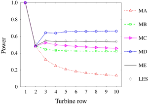
Figure 5. Normalized power production for different turbine rows.
Figure 5 shows the normalized power production of each turbine row (denoted as  $\overline{P_{i}}$), at a representative wind direction of
  $\unicode[STIX]{x1D703}=270^{\circ }$. As indicated by the LES results, the power production first drops and then remains approximately unchanged. The proposed new method, once again, outperforms the other methods by closely following the trend stipulated by LES. For Methods A and C, since the individual wake velocity deficits are directly summed, the total wake velocity deficit keeps accumulating unrealistically in the streamwise direction, leading to a decreasing trend of the power production. As a comparison, for Methods B and D, due to the usage of a square-sum operation in the combination of individual wake velocity deficits, the predicted power production quickly reaches a plateau after three turbine rows. Nevertheless, this plateau value deviates noticeably from that in the LES results.
4 Extension to wake deflection superposition
Active wake control has been increasingly recognized as an effective technique to mitigate the unfavourable wake interactions in wind farms. Bay et al. (Reference Bay, King, Fleming, Mudafort and Martinez2019) demonstrated that, to accurately predict the power production subject to active wake control, it is crucial to include the ‘secondary steering effect’ sketched in figure 6(a), where, as the upstream wind turbine  $\text{WT}_{1}$ yaws, the wake trajectory of a non-yawed downstream wind turbine
  $\text{WT}_{2}$ deviates from its rotor centreline. This unexpected wake deflection, originating from the non-vanishing transverse velocity induced by
  $\text{WT}_{1}$ at the position of
  $\text{WT}_{2}$, underlies the necessity of wake deflection superposition. Starting from the simplified spanwise momentum equation derived in appendix (A 4) and following a similar procedure as described in § 2, the superposition principle of
  $v^{i}$ can be derived, as follows:
 $$\begin{eqnarray}V(x,y,z)=\mathop{\sum }_{i}\frac{u_{c}^{i}(x)}{U_{c}(x)}v^{i}(x,y,z),\end{eqnarray}$$
 where  $V$ is the spatially dependent transverse velocity for the combined wake. This equation, together with (2.9), reiterates that a weighed sum should be used to combine the individual transverse velocity/wake velocity deficits, instead of a direct sum.

Figure 6. (a) Sketch of the secondary steering effect. The wake trajectories of  $\text{WT}_{1}$ and
  $\text{WT}_{2}$ are indicated by the solid lines. (b) Wake velocity fields measured at the hub level. Top plot (Case 1):
  $\unicode[STIX]{x1D6FD}_{1}=30^{\circ },\unicode[STIX]{x1D6FD}_{2}=0^{\circ },\unicode[STIX]{x1D6FD}_{2}=0^{\circ }$. Bottom plot (Case 2):
  $\unicode[STIX]{x1D6FD}_{1}=30^{\circ },\unicode[STIX]{x1D6FD}_{2}=20^{\circ },\unicode[STIX]{x1D6FD}_{2}=0^{\circ }$. The red solid lines and the white dash-dot lines represent the wake trajectories extracted from PIV data and computed by (4.3), respectively.
In the current wake models of yawed wind turbines, the wake deflection is typically integrated from the slope of the wake trajectory, defined as the ratio of the wake-centre transverse velocity to the mean convection velocity, as sketched in figure 6(a). Following this route and applying (4.1) to the wake centre of the  $j$th wind turbine
  $(x_{c}^{j},y_{c}^{j})$, the total transverse velocity experienced by the wake of
  $\text{WT}_{j}$ (
 $V_{c}^{j}$) can be obtained:
 $$\begin{eqnarray}V_{c}^{j}(x_{c}^{j},y_{c}^{j})=\mathop{\sum }_{i}\frac{u_{c}^{i}(x_{c}^{j})}{U_{c}(x_{c}^{j})}v^{i}(x_{c}^{j},y_{c}^{j}).\end{eqnarray}$$
 It is evident from (4.2) that, in order to derive the total wake deflection, the mean convection velocity for the combined wake ( $U_{c}$) has to be known a priori, which is impossible as
  $U_{c}$ is dependent on the spatial distributions of the individual wake velocity deficits and thus can only be computed once the wake deflection is given. In principle, an iterative method should be deployed to reconcile this conflict. However, to avoid increasing the computational cost,
  $u_{c}^{i}/U_{c}$ is approximated by
  $u_{0}^{i}/u_{0}^{j}$, and the slope of the wake trajectory of
  $\text{WT}_{j}$ is written as
 $$\begin{eqnarray}\frac{\text{d}y_{c}^{j}}{\text{d}x_{c}^{j}}\approx \frac{V_{c}^{j}}{u_{0}^{j}}\approx \mathop{\sum }_{i}\frac{u_{0}^{i}}{u_{0}^{j}u_{0}^{j}}v^{i}(x_{c}^{j},y_{c}^{j}).\end{eqnarray}$$
 Currently, several models are available to compute the transverse velocity induced by a stand-alone yawed wind turbine (i.e.  $v^{i}$) (Jiménez, Crespo & Migoya Reference Jiménez, Crespo and Migoya2010; Bastankhah & Porté-Agel Reference Bastankhah and Porté-Agel2016; Shapiro et al. Reference Shapiro, Gayme and Meneveau2018). For the sake of simplicity, the following expression adapted from Shapiro et al. (Reference Shapiro, Gayme and Meneveau2018) is used in this investigation:
 $$\begin{eqnarray}v^{i}(x,y)=\frac{-C_{t}^{i}u_{0}^{i}\cos ^{2}\unicode[STIX]{x1D6FD}_{i}\sin \unicode[STIX]{x1D6FD}_{i}}{8\unicode[STIX]{x1D70E}_{y}\unicode[STIX]{x1D70E}_{z}/\unicode[STIX]{x1D70E}_{y0}\unicode[STIX]{x1D70E}_{z0}}\cdot \left[1+\text{erf}\left(\frac{x}{D}\right)\right]\cdot \exp \left(-\frac{(y-y_{c}^{i})^{2}}{2\unicode[STIX]{x1D70E}_{y}^{2}}\right),\end{eqnarray}$$
 where  $\unicode[STIX]{x1D70E}_{y0}$ and
  $\unicode[STIX]{x1D70E}_{z0}$ are the initial wake widths along the spanwise and vertical directions, respectively. Different from the original expression, a Gaussian function (i.e.
  $\exp (-(y-y_{c}^{i})^{2}/2\unicode[STIX]{x1D70E}_{y}^{2})$) is added here, to spread the transverse velocity in the spanwise direction and thus generalize the wake deflection superposition to partial wake conditions.
The three-row model wind farm described in § 3.1 is used once again as a test bench to validate the proposed method of wake deflection superposition. Two cases are selected to execute PIV measurements. In the first case, only the most upstream wind turbine is yawed at  $\unicode[STIX]{x1D6FD}_{1}=30^{\circ }$. In the second case, both
  $\text{WT}_{1}$ and
  $\text{WT}_{2}$ are actuated, and the optimal yaw angle list for the maximum power production (
 $\unicode[STIX]{x1D6FD}_{1}=30^{\circ },\unicode[STIX]{x1D6FD}_{2}=20^{\circ },\unicode[STIX]{x1D6FD}_{3}=0^{\circ }$) reported in Bastankhah & Porté-Agel (Reference Bastankhah and Porté-Agel2019) is adopted. Figure 6(b) compares the wake trajectories extracted from the PIV measurements and obtained by (4.3). In both cases, the secondary steering effect is successfully reproduced by the proposed analytical method, and the wake deflections of the first two wind turbines (
 $y_{c}$) are predicted within a mean error of less than
  $0.05D$. For the last wind turbine, the measured wake deflection is higher than the model prediction, which can be attributed to the spanwise wind shear. Specifically, when the wake of
  $\text{WT}_{2}$ shifts preferably to the negative
  $y$-direction, the lower half of
  $\text{WT}_{3}$ perceives a lower wind speed than the upper half. Due to this noticeable wind shear, different levels of turbulent kinetic energy are generated on the two sides of the wake of
  $\text{WT}_{3}$, leading to uneven wake recovery rates. As a result, larger/smaller wake velocity deficits are exhibited on the side with a lower/higher wake recovery rate, resulting in an additional shift of the wake centre, independent from that caused by the non-vanishing transverse velocity induced by the upstream yawed wind turbines.
5 Summary
In this study, a novel wake superposition method is derived rigorously from the law of conservation of momentum. The total wake velocity deficit is expressed as a weighted sum of the individual wake velocity deficits, where the weight equals to the ratio of the characteristic convection velocity of the individual wake to that of the combined wake. The performance of this new method is validated against the PIV data obtained in a three-row model wind farm and the LES results pertaining to the Horns-Rev wind farm. Detailed comparisons show that, except for the near-wake region where the pressure gradient is non-trivial, the proposed wake superposition method can give a rather accurate prediction of the centreline wake velocity deficit. The maximum power prediction error in the case of the Horns-Rev wind farm is reduced to as low as 5 %. None of the wake superposition methods available in the literature is able to achieve such a high accuracy, largely because of their inability to conserve the total momentum deficit during wake superposition. Additionally, the momentum-conserving wake superposition principle has been extended to combine the transverse velocities induced by yawed wind turbines, and the secondary wake steering effect crucial to active wake control is successfully reproduced.
Acknowledgements
This research was funded by the Swiss National Science Foundation (grant number: 200021_172538) and the Swiss Federal Office of Energy. In addition, this project was carried out within the frame of the Swiss Centre for Competence in Energy Research on the Future Swiss Electrical Infrastructure (SCCER-FURIES) with the financial support of the Swiss Innovation Agency (Innosuisse – SCCER programme, contract number: 1155002544).
Declaration of interests
The authors report no conflict of interest.
Appendix A. Simplified momentum equations for wake flow
A sufficiently large stream tube enclosing the entire wind turbine is selected as the control volume, as sketched in figure 7. Only uniform inflow is considered, which is one of the inherent assumptions made to derive the analytical wind turbine wake models (Jensen Reference Jensen1983; Frandsen et al. Reference Frandsen, Barthelmie, Pryor, Rathmann, Larsen, Højstrup and Thøgersen2006; Bastankhah & Porté-Agel Reference Bastankhah and Porté-Agel2014). The inlet of the stream tube is placed far away from the induction zone of the turbine, such that both the static pressure and the inlet velocity remain unaffected and can be treated as ambient values of  $p=p_{0}$ and
  $u=u_{0}$. Similarly, the outlet is positioned in the far wake, where the static pressure deviates marginally from the ambient pressure, i.e.
  $p\approx p_{0}$. The turbulent momentum transportation contributed by the Reynolds normal stress term
  $\langle u^{\prime }u^{\prime }\rangle$ is typically small compared to the mean momentum transportation (
 $O(u_{0}^{2})$), and, thus, can be readily neglected (Tennekes & Lumley Reference Tennekes and Lumley1972). In addition, since the stream tube is selected to be sufficiently large, the pressure disturbances and turbulent shear stresses generated by wakes will not be felt by the side boundaries, leading to zero pressure force and zero turbulent momentum transfer in the spanwise and vertical directions, i.e.
  $\langle u^{\prime }v^{\prime }\rangle \approx 0$ and
  $\langle u^{\prime }w^{\prime }\rangle \approx 0$.

Figure 7. The control volume and boundary conditions used to derive the simplified momentum equations for wake flow.
Based on the above assumptions, the integral form of the streamwise momentum equation (Anderson Reference Anderson2010), when applied to the control volume shown in figure 7, can be simplified as follows:
 $$\begin{eqnarray}\unicode[STIX]{x1D70C}\iint _{inlet}u_{0}^{2}\,\text{d}y\,\text{d}z-\unicode[STIX]{x1D70C}\iint _{outlet}u_{w}(x,y,z)^{2}\,\text{d}y\,\text{d}z=T,\end{eqnarray}$$
 where  $T$ denotes the turbine thrust in the streamwise direction. Essentially, equation (A 1) states that the total momentum difference between the inlet and outlet of the stream tube equals the drag imposed to the flow. Further, applying the law of conservation of mass to the control volume, we have
 $$\begin{eqnarray}\unicode[STIX]{x1D70C}\iint _{inlet}u_{0}\,\text{d}y\,\text{d}z=\unicode[STIX]{x1D70C}\iint _{outlet}u_{w}(x,y,z)\,\text{d}y\,\text{d}z.\end{eqnarray}$$
Substituting (A 2) into (A 1), the following expression can be obtained:
 $$\begin{eqnarray}T=\unicode[STIX]{x1D70C}\iint _{outlet}u_{w}(x,y,z)\cdot u_{s}(x,y,z)\,\text{d}y\,\text{d}z.\end{eqnarray}$$
 In the case of a yawed wind turbine, a similar expression for the lateral turbine thrust (denoted as  $F$) can be derived from the spanwise momentum equation. In particular, there is no spanwise momentum flowing into the control volume, and the total spanwise momentum integrated over the outlet is directly balanced out by the lateral force
  $F$, which reads as
 $$\begin{eqnarray}F=\unicode[STIX]{x1D70C}\iint _{outlet}u_{w}(x,y,z)\cdot v(x,y,z)\,\text{d}y\,\text{d}z.\end{eqnarray}$$


