


1 Introduction
Flow-induced motion, deformation and breakup of droplets on a solid surface have been the subject of intense research because of their scientific and technical importance (Dimitrakopoulos & Higdon Reference Dimitrakopoulos and Higdon1998; Spelt Reference Spelt2006; Dimitrakopoulos Reference Dimitrakopoulos2007; Ding & Spelt Reference Ding and Spelt2008; Gupta & Basu Reference Gupta and Basu2008; Sugiyama & Sbragaglia Reference Sugiyama and Sbragaglia2008; Ding, Gilani & Spelt Reference Ding, Gilani and Spelt2010). In many applications involving droplets on a solid surface, surfactants are often present as impurities or are added deliberately to the bulk fluid, which can critically affect the dynamics of multiphase flow systems. For example, in the petroleum industry, enhanced oil recovery depends strongly on the displacement of oil droplets through rock formation, and surfactants are commonly used to increase oil production by decreasing the interfacial tension between fluids and altering the wetting properties of rock surfaces (Shah & Schechter Reference Shah and Schechter2012; Hou et al. Reference Hou, Wang, Cao, Zhang, Song, Ding and Chen2016; Wei et al. Reference Wei, Hou, Sukop and Liu2019). In the coating industry, surfactants can mitigate the wetting failure (Schunk & Scriven Reference Schunk and Scriven1997; Liu et al. Reference Liu, Vandre, Carvalho and Kumar2016a,Reference Liu, Vandre, Carvalho and Kumarb), which occurs when the liquid no longer entirely displaces the ambient gas at the contact line, thus improving the uniformity required for precision film coating. Recently, rapid developments in microfluidic technologies have enabled reliable fabrication and manipulation of small droplets with controlled size using low-cost devices, where the addition of surfactants is essential to stabilise the droplets against coalescence (Binks et al. Reference Binks, Fletcher, Holt, Beaussoubre and Wong2010; Li, Wang & Luo Reference Li, Wang and Luo2017; Zinchenko & Davis Reference Zinchenko and Davis2017; Riaud et al. Reference Riaud, Zhang, Wang, Wang and Luo2018; Roumpea et al. Reference Roumpea, Kovalchuk, Chinaud, Nowak, Simmons and Angeli2019).
There have been a number of experimental studies investigating the motion of a liquid droplet on a solid surface in the presence of surfactants (Rafaïet al. Reference Rafaï, Sarker, Bergeron, Meunier and Bonn2002; Tan, Gee & Stevens Reference Tan, Gee and Stevens2003; Nikolov & Wasan Reference Nikolov and Wasan2015; Jiang, Sun & Santamarina Reference Jiang, Sun and Santamarina2016; Roumpea et al. Reference Roumpea, Kovalchuk, Chinaud, Nowak, Simmons and Angeli2019). Nevertheless, it is still very challenging to conduct precise experimental measurements of the local surfactant concentration and flow fields during the droplet movement, and experimental studies suffer from the difficulty to assess the effect of each influencing factor. Theoretical studies based on a lubrication approximation have been used for analysing the spreading and stability of a surfactant-covered droplet with a sufficiently small aspect ratio (defined by the maximum height of the droplet to its length) on a substrate (Clay & Miksis Reference Clay and Miksis2004; Jensen & Naire Reference Jensen and Naire2006; Karapetsas, Craster & Matar Reference Karapetsas, Craster and Matar2011a,Reference Karapetsas, Craster and Matarb; Weidner Reference Weidner2012; Wei Reference Wei2018). Unfortunately, they are unable to solve the instantaneous behaviour of a spherical cap droplet with a large contact angle due to the limitation of lubrication approximation. Numerical simulations can complement theoretical and experimental studies, providing additional insights into how the flow and physical parameters influence the dynamical behaviours of droplets on a solid surface in the presence of surfactants.
The efficient and accurate computational modelling of droplet motion on a solid surface with surfactants is a challenging task. The surfactant concentration at the interface alters the interfacial tension locally, and a non-uniform distribution of surfactants creates non-uniform capillary forces and tangential Marangoni stresses, which affect the flow field in a complicated manner. In turn, the flow field advects the surfactants and influences their distribution, causing the surfactant concentration and flow field to couple. From a numerical point of view, the surfactant evolution equation must be solved together with the hydrodynamic equations at moving and deforming interfaces, which may undergo topological changes such as breakup and coalescence. In addition, when the droplet moves over a solid surface, the contact angle should dynamically vary with the local surfactant concentration and the moving contact lines (MCL) need to be handled properly, which have for many years remained an issue of controversy and debate (Sui, Ding & Spelt Reference Sui, Ding and Spelt2014), posing an additional numerical challenge.
To tackle the aforementioned challenges, many efforts have been dedicated to the study of interfacial flows with both surfactants and contact-line dynamics. Yon & Pozrikidis (Reference Yon and Pozrikidis1999) studied the effect of insoluble surfactants on a droplet attached to a plane wall and subject to an overpassing shear flow in the limit of Stokes flow. To simplify the problem, they assumed that the contact line retains a circular shape and pins on the solid surface during the droplet deformation. Their results revealed that the overall behaviour of the droplet is determined not only by the capillary number and viscosity ratio, but also by the sensitivity of interfacial tension to variations in surfactant concentration. Schleizer & Bonnecaze (Reference Schleizer and Bonnecaze1999) presented a boundary-integral method to investigate the role of surfactants on the displacement of a two-dimensional (2-D) immiscible droplet over a solid wall in both shear and pressure-driven flows. They considered the contact lines either fixed or mobile, and assumed that, when the contact lines are allowed to move, the contact angle is independent of the slip velocity and is therefore equal to its static value. They found that for a neutral surface the critical capillary number, above which the droplet cannot reach a steady shape, is larger for droplets with MCL compared to those with pinned contact lines. Axisymmetric spreading of a liquid droplet containing soluble surfactants on an ideal substrate was numerically investigated by Chan & Borhan (Reference Chan and Borhan2006), where the slip velocity of a contact line was related to the dynamic contact angle through a constitutive equation. Lai, Tseng & Huang (Reference Lai, Tseng and Huang2010) developed an immersed boundary method to simulate a droplet on a solid substrate under the influence of insoluble surfactants. An unbalanced Young stress, resulting from the deviation of the dynamic contact angle from the static one, was incorporated into the momentum equations as a driving force for the contact-line motion. An arbitrary Lagrangian–Eulerian finite element scheme for a soluble surfactant droplet impingement on a horizontal surface was presented by Ganesan (Reference Ganesan2013). In his work, the dynamic contact angle was expressed as a function of the static contact angle and the local surfactant concentration. Xu & Ren (Reference Xu and Ren2014) presented a level-set method for the simulation of two-phase flows with insoluble surfactants and MCL. A contact angle condition, which relates the unbalanced Young stress to the slip velocity of the contact line, was used to include the effect of surfactants on surface wettability. By decomposing the fluid interface into segments with local Eulerian grids, af Klinteberg, Lindbo & Tornberg (Reference af Klinteberg, Lindbo and Tornberg2014) developed a numerical method for two-phase flows with insoluble surfactants and contact-line dynamics in two dimensions. To drive the movement of the contact line, they defined the tangential velocity in the vicinity of the contact line and used the Navier slip condition on the walls away from the contact line. Based on thermodynamic principles, Zhang, Xu & Ren (Reference Zhang, Xu and Ren2014) derived a continuous model for the dynamics of two immiscible fluids with MCL and insoluble surfactants, in which the condition for the dynamic contact angle was obtained by the consideration of energy dissipations. Recently, we presented a lattice-Boltzmann (LB) and finite-difference hybrid method for the simulation of a 2-D droplet moving on a solid wall subject to a linear shear flow (Zhang, Liu & Ba Reference Zhang, Liu and Ba2019). To model the fluid–surface interactions, a dynamic contact angle formulation that describes the dependence of the local contact angle on the surfactant concentration was derived, and the resulting contact angle was enforced by a geometrical wetting condition. By comparing a clean droplet with a surfactant-covered droplet at the same effective capillary number ( $Ca_{e}$), we explored, for the first time, how the presence of surfactants influences the droplet motion, deformation and breakup for varying
  $Ca_{e}$. Wei et al. (Reference Wei, Hou, Sukop and Liu2019) conducted a pore-scale study of ternary amphiphilic fluid flow through a porous media using a bottom-up LB model, in which a dipole is introduced to capture the amphiphilic structure of surfactant molecules. It was found that surfactants could improve the oil recovery in all wetting conditions, but the surfactant loss due to adsorption onto walls diminishes the effect of interfacial tension reduction. In addition, Tang et al. (Reference Tang, Xiao, Lei, Yuan, Peng, He, Luo and Pei2019) carried out molecular dynamics simulations to study the surfactant flooding driven detachment of oil droplet in a nanosilica channel. They revealed that the surfactant molecules tend to migrate to the rear bottom of the oil molecular aggregate caused by the water flow effect and hydration of polar head groups of surfactants, which facilitate the penetration of water molecules into the oil–rock interface, and the oil molecule detachment occurs at the rear bottom of the oil molecular aggregate.
As reviewed above, most of the studies focus on developing numerical methods for computation of interfacial flows with both surfactants and contact-line dynamics, but these methods are not applicable when the local surfactant concentration approaches or exceeds the critical micelle concentration (CMC, at which surfactant molecules begin to self-associate to form stable aggregates known as micelles). In addition, although several works have studied the dynamical behaviour of a surfactant-covered droplet on a solid surface subject to a shear flow, e.g. Schleizer & Bonnecaze (Reference Schleizer and Bonnecaze1999), Yon & Pozrikidis (Reference Yon and Pozrikidis1999), Zhang et al. (Reference Zhang, Liu and Ba2019), they commonly suffer from the following drawbacks: (I) they either have not considered the MCL or are limited to two dimensions, which cannot reproduce the physical three-dimensional test conditions accurately; (II) the factors influencing the droplet motion and deformation have not yet been studied systematically; and (III) the critical conditions of droplet breakup, e.g. for varying viscosity ratio, have been rarely explored so far.
In this work we will extend our recently developed hybrid method to three dimensions for the simulation of a surfactant-covered droplet moving on a solid surface subject to a linear shear flow, where the droplet is of equal density to the ambient fluid and the Reynolds number is fixed at 1. Unlike its 2-D counterpart (Zhang et al. Reference Zhang, Liu and Ba2019), the present method is able to deal with the surfactant concentration beyond the CMC. In order to break the limitations of the existing works, we will study not only the droplet deformation and motion for varying effective capillary number, viscosity ratio and surfactant coverage, but also the critical conditions of droplet breakup for varying viscosity ratio, in which the roles of surfactants will be identified by comparing with the results of a clean droplet. The paper is organised as follows. In § 2 the mathematical model and numerical method are described briefly, and in § 3 the results of droplet motion, deformation and breakup are presented and discussed. The paper closes with a summary of the main results in § 4.
2 Problem statement and numerical method
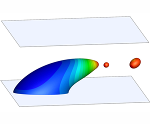
We consider the dynamical behaviour of a surfactant-covered droplet moving on a solid surface and subject to a three-dimensional (3-D) linear shear flow. As sketched in figure 1, two infinite walls, both parallel to the  $x$–
$x$– $y$ plane, are separated by a distance
  $H$. The bottom wall is stationary, and the top wall moves to the right with a constant velocity
  $u_{w}$, thus creating a shear flow with the shear rate
  $\dot{\unicode[STIX]{x1D6FE}}=u_{w}/H$. Initially, a hemispherical droplet (red fluid) with the radius of
  $R$ rests on the bottom wall. Both droplet and ambient fluid (blue fluid) are assumed to be incompressible, viscous and immiscible, and to have equal densities. The dynamic viscosities for the droplet and ambient fluid are
  $\unicode[STIX]{x1D707}^{R}$ and
  $\unicode[STIX]{x1D707}^{B}$, respectively. For the sake of simplicity, the surfactants are considered to be insoluble and present only at the interface between the droplet and the ambient fluid, and they are initially distributed uniformly at the droplet surface with a concentration of
  $\unicode[STIX]{x1D713}_{0}$.

Figure 1. A hemispherical droplet sitting on a solid wall subject to a linear shear flow. The shear flow is created by moving the top wall with a constant velocity  $u_{w}$. The computational domain has a size of
  $L\times W\times H=560\times 400\times 100$, and the droplet has an initial radius of
  $R=50$. The droplet and the ambient fluid are assumed to have equal densities, and their dynamic viscosities are
  $\unicode[STIX]{x1D707}^{R}$ and
  $\unicode[STIX]{x1D707}^{B}$, which give a viscosity ratio of
  $\unicode[STIX]{x1D706}=\unicode[STIX]{x1D707}^{R}/\unicode[STIX]{x1D707}^{B}$.
Using the continuum surface force formulation, the fluid flow for such a multiphase system is governed by a single set of Navier–Stokes equations (NSE):
 $$\begin{eqnarray}\displaystyle & \displaystyle \unicode[STIX]{x1D735}\boldsymbol{\cdot }\boldsymbol{u}=0, & \displaystyle\end{eqnarray}$$
 $$\begin{eqnarray}\displaystyle & \displaystyle \unicode[STIX]{x2202}_{t}(\unicode[STIX]{x1D70C}\boldsymbol{u})+\unicode[STIX]{x1D735}\boldsymbol{\cdot }(\unicode[STIX]{x1D70C}\boldsymbol{u}\boldsymbol{u})=-\unicode[STIX]{x1D735}p+\unicode[STIX]{x1D735}\boldsymbol{\cdot }[\unicode[STIX]{x1D707}(\unicode[STIX]{x1D735}\boldsymbol{u}+\unicode[STIX]{x1D735}\boldsymbol{u}^{\text{T}})]+\boldsymbol{F}_{s}, & \displaystyle\end{eqnarray}$$
 where  $t$ is the time,
  $\unicode[STIX]{x1D707}$ is the dynamic viscosity and
  $\unicode[STIX]{x1D70C}$,
  $\boldsymbol{u}$ and
  $p$ are the total density, fluid velocity and pressure, respectively. The last term in (2.2) represents the interfacial force which includes not only the interfacial tension force but also the Marangoni stress, and is defined as
 $$\begin{eqnarray}\boldsymbol{F}_{s}=\unicode[STIX]{x1D70E}\unicode[STIX]{x1D705}\boldsymbol{n}\unicode[STIX]{x1D6FF}_{\unicode[STIX]{x1D6E4}}+\unicode[STIX]{x1D6FF}_{\unicode[STIX]{x1D6E4}}\unicode[STIX]{x1D735}_{s}\unicode[STIX]{x1D70E},\end{eqnarray}$$
 where  $\unicode[STIX]{x1D70E}$ is the interfacial tension,
  $\unicode[STIX]{x1D705}$ is the interface curvature,
  $\boldsymbol{n}$ is the unit normal to the interface,
  $\unicode[STIX]{x1D735}_{s}=\unicode[STIX]{x1D735}-\boldsymbol{n}(\boldsymbol{n}\boldsymbol{\cdot }\unicode[STIX]{x1D735})$ is the surface gradient operator and
  $\unicode[STIX]{x1D6FF}_{\unicode[STIX]{x1D6E4}}$ is the Dirac delta function which should satisfy
  $\int _{-\infty }^{\infty }\unicode[STIX]{x1D6FF}_{\unicode[STIX]{x1D6E4}}\text{d}\unicode[STIX]{x1D712}=1$ in order to recover properly the stress jump condition in the sharp-interface limit. Here
  $\unicode[STIX]{x1D712}$ is the spatial location normal to the interface.
In addition to (2.1) and (2.2), an advection equation has to be solved to capture the interface evolution in traditional multiphase solvers, e.g. the volume-of-fluid and level-set methods, where the sophisticated interface reconstruction algorithm or unphysical reinitialization process is often required. In order to avoid these issues, we use an improved LB colour-gradient model for immiscible two-phase flows with variable interfacial tension, where the surfactant concentration can be above the CMC. In the colour-gradient model, the red and blue distribution functions  $f_{i}^{R}$ and
  $f_{i}^{B}$ are introduced to represent the droplet and the ambient fluid, respectively. The implementation of this model consists of three steps, i.e. collision, recolouring and streaming. The recolouring and streaming steps are exactly the same as those in Liu et al. (Reference Liu, Ba, Wu, Li, Xi and Zhang2018) and thus are not shown here. For the collision step, the total distribution function
  $f_{i}=f_{i}^{R}+f_{i}^{B}$ evolves as
 $$\begin{eqnarray}f_{i}^{\dagger }(\boldsymbol{x},t)=f_{i}(\boldsymbol{x},t)+\unicode[STIX]{x1D6FA}_{i}(\boldsymbol{x},t)+\bar{F_{i}},\end{eqnarray}$$
 where  $f_{i}(\boldsymbol{x},t)$ is the total distribution function in the
  $i$th velocity direction at the position
  $\boldsymbol{x}$ and time
  $t$,
$t$,  $f_{i}^{\dagger }(\boldsymbol{x},t)$ is the post-collision total distribution function,
  $\unicode[STIX]{x1D6FA}_{i}(\boldsymbol{x},t)$ is the collision operator and
  $\bar{F_{i}}$ is the forcing term.
To obtain viscosity-independent wall location and contact-line dynamics, the multiple-relaxation-time collision operator is adopted instead of its Bhatnagar–Gross–Krook counterpart, and is given by (Zhang et al. Reference Zhang, Liu and Ba2019)
 $$\begin{eqnarray}\unicode[STIX]{x1D6FA}_{i}(\boldsymbol{x},t)=-\mathop{\sum }_{j}(\unicode[STIX]{x1D648}^{-1}\unicode[STIX]{x1D64E}\unicode[STIX]{x1D648})_{ij}(f_{j}(\boldsymbol{x},t)-f_{j}^{eq}(\boldsymbol{x},t)),\end{eqnarray}$$
 where  $\unicode[STIX]{x1D648}$ is the transformation matrix that linearly maps the distribution functions onto their moments and
  $\unicode[STIX]{x1D64E}$ is a diagonal relaxation matrix. Here
  $f_{i}^{eq}$ is the equilibrium distribution function defined as
 $$\begin{eqnarray}f_{i}^{eq}=\unicode[STIX]{x1D70C}w_{i}\left[1+\frac{\boldsymbol{e}_{i}\boldsymbol{\cdot }\boldsymbol{u}}{c_{s}^{2}}+\frac{(\boldsymbol{e}_{i}\boldsymbol{\cdot }\boldsymbol{u})^{2}}{2c_{s}^{4}}-\frac{\boldsymbol{u}^{2}}{2c_{s}^{2}}\right],\end{eqnarray}$$
 where  $\unicode[STIX]{x1D70C}$ is calculated by
  $\unicode[STIX]{x1D70C}=\unicode[STIX]{x1D70C}^{R}+\unicode[STIX]{x1D70C}^{B}$ with the superscripts ‘
 $R$’ and ‘
 $B$’ referring to the droplet and ambient fluid respectively,
  $\boldsymbol{e}_{i}$ is the lattice velocity in the
  $i$th direction,
  $w_{i}$ is the weighting factor and
  $c_{s}$ is the speed of sound. For the 3-D 19-velocity (D3Q19) lattice model used in the present study, the speed of sound
  $c_{s}=\unicode[STIX]{x1D6FF}_{x}/(\sqrt{3}\unicode[STIX]{x1D6FF}_{t})=1/\sqrt{3}$, where the lattice spacing
  $\unicode[STIX]{x1D6FF}_{x}$ and the time step
  $\unicode[STIX]{x1D6FF}_{t}$ are both taken as 1, and the explicit expressions of
  $\unicode[STIX]{x1D648}$,
  $\boldsymbol{e}_{i}$ and
  $w_{i}$ can be found in D’humières et al. (Reference D’humières, Ginzburg, Krafczyk, Lallemand and Luo2002).
The diagonal relaxation matrix  $\unicode[STIX]{x1D64E}$ reads as (Ginzburg & d’Humières Reference Ginzburg and d’Humières2003; Wang, Liu & Zhang Reference Wang, Liu and Zhang2017)
 $$\begin{eqnarray}\unicode[STIX]{x1D64E}=\text{diag}\left[0,s_{1},s_{2},0,s_{4},0,s_{4},0,s_{4},s_{9},s_{10},s_{9},s_{10},s_{13},s_{13},s_{13},s_{16},s_{16},s_{16}\right],\end{eqnarray}$$
 with the relaxation rates  $s_{i}$ given as
 $$\begin{eqnarray}s_{1}=s_{2}=s_{9}=s_{10}=s_{13}=\unicode[STIX]{x1D714},\quad s_{4}=s_{16}=\frac{8(2-s_{1})}{8-s_{1}},\end{eqnarray}$$
 where  $\unicode[STIX]{x1D714}$ is the dimensionless relaxation parameter related to the dynamic viscosity
  $\unicode[STIX]{x1D707}$ by
  $\unicode[STIX]{x1D707}=(1/\unicode[STIX]{x1D714}-0.5)\unicode[STIX]{x1D70C}c_{s}^{2}\unicode[STIX]{x1D6FF}_{t}$. To account for unequal viscosities of the two fluids, the dynamic viscosity
  $\unicode[STIX]{x1D707}$ is determined by the harmonic mean as
 $$\begin{eqnarray}\frac{1}{\unicode[STIX]{x1D707}}=\frac{1+\unicode[STIX]{x1D70C}^{N}}{2\unicode[STIX]{x1D707}^{R}}+\frac{1-\unicode[STIX]{x1D70C}^{N}}{2\unicode[STIX]{x1D707}^{B}},\end{eqnarray}$$
 where  $\unicode[STIX]{x1D70C}^{N}$ is the phase field function responsible to identify the interface location, and is defined by
 $$\begin{eqnarray}\unicode[STIX]{x1D70C}^{N}(\boldsymbol{x},t)=\frac{\unicode[STIX]{x1D70C}^{R}(\boldsymbol{x},t)-\unicode[STIX]{x1D70C}^{B}(\boldsymbol{x},t)}{\unicode[STIX]{x1D70C}^{R}(\boldsymbol{x},t)+\unicode[STIX]{x1D70C}^{B}(\boldsymbol{x},t)}.\end{eqnarray}$$
The CMC is the surfactant concentration above which surfactant molecules aggregate to form micelles, and it is an important parameter that characterises the surfactant behaviour. Before reaching the CMC, the interfacial tension decreases rapidly with the surfactant concentration, and the Langmuir equation of state can be adopted to describe the relation between the surfactant concentration and the interfacial tension. However, after reaching the CMC, the interfacial tension changes slowly with the surfactant concentration or even remains a constant (Zhao et al. Reference Zhao, Zhang, Xu, Li and Liu2017; Kovalchuk et al. Reference Kovalchuk, Roumpea, Nowak, Chinaud, Angeli and Simmons2018). To allow for surfactant concentration beyond the CMC, a modified Langmuir equation of state is often used and it reads as (Pawar & Stebe Reference Pawar and Stebe1996; Young et al. Reference Young, Booty, Siegel and Li2009; Ngangia et al. Reference Ngangia, Young, Vlahovska and Blawzdziewicz2013)
 $$\begin{eqnarray}\unicode[STIX]{x1D70E}(\unicode[STIX]{x1D713})=\max \{\unicode[STIX]{x1D70E}_{0}[1+E_{0}\ln (1-\unicode[STIX]{x1D713}/\unicode[STIX]{x1D713}_{\infty })],\unicode[STIX]{x1D70E}_{min}\},\end{eqnarray}$$
 where  $\unicode[STIX]{x1D713}_{\infty }$ is the surfactant concentration at the maximum packing,
  $\unicode[STIX]{x1D70E}_{0}$ is the interfacial tension of a clean interface (i.e.
  $\unicode[STIX]{x1D713}=0$),
  $E_{0}$ is the elasticity number that measures the sensitivity of
  $\unicode[STIX]{x1D70E}$ to the variation of
  $\unicode[STIX]{x1D713}$ and
  $\unicode[STIX]{x1D70E}_{min}$ is the interfacial tension after reaching the CMC. Note that the value of
  $\unicode[STIX]{x1D70E}_{min}$ varies for different combinations of fluids and surfactants. In the present study, we follow the previous works (De Bruijn Reference De Bruijn1993; Ngangia et al. Reference Ngangia, Young, Vlahovska and Blawzdziewicz2013) to simply take
  $\unicode[STIX]{x1D70E}_{min}=\unicode[STIX]{x1D70E}_{0}/10$. The value of CMC, according to its definition, can be computed by equating the two terms in max function. As previously done by Xu et al. (Reference Xu, Li, Lowengrub and Zhao2006) and Liu et al. (Reference Liu, Ba, Wu, Li, Xi and Zhang2018), we also quantify the initial average surfactant concentration
  $\unicode[STIX]{x1D713}_{0}$ through the surfactant coverage, which is defined as
  $x_{in}=\unicode[STIX]{x1D713}_{0}/\unicode[STIX]{x1D713}_{\infty }$.
By defining  $\boldsymbol{n}=-\unicode[STIX]{x1D735}\unicode[STIX]{x1D70C}^{N}/|\unicode[STIX]{x1D735}\unicode[STIX]{x1D70C}^{N}|$ and
  $\unicode[STIX]{x1D6FF}_{\unicode[STIX]{x1D6E4}}=|\unicode[STIX]{x1D735}\unicode[STIX]{x1D70C}^{N}|/2$ and substituting the above equation of state, (2.3) can be further written as
 $$\begin{eqnarray}\boldsymbol{F}_{s}=\left\{\begin{array}{@{}ll@{}}\displaystyle -\frac{1}{2}\unicode[STIX]{x1D70E}\unicode[STIX]{x1D705}\unicode[STIX]{x1D735}\unicode[STIX]{x1D70C}^{N}-\frac{1}{2}|\unicode[STIX]{x1D735}\unicode[STIX]{x1D70C}^{N}|\frac{\unicode[STIX]{x1D70E}_{0}E_{0}}{\unicode[STIX]{x1D713}_{\infty }-\unicode[STIX]{x1D713}}\left[\unicode[STIX]{x1D735}\unicode[STIX]{x1D713}-(\boldsymbol{n}\boldsymbol{\cdot }\unicode[STIX]{x1D735}\unicode[STIX]{x1D713})\boldsymbol{n}\right], & \unicode[STIX]{x1D713}<\text{CMC},\\ \displaystyle -\frac{1}{2}\unicode[STIX]{x1D70E}\unicode[STIX]{x1D705}\unicode[STIX]{x1D735}\unicode[STIX]{x1D70C}^{N}, & \unicode[STIX]{x1D713}\geqslant \text{CMC},\end{array}\right.\end{eqnarray}$$
 where the interface curvature  $\unicode[STIX]{x1D705}$ is related to
  $\boldsymbol{n}$ by
  $\unicode[STIX]{x1D705}=-\unicode[STIX]{x1D735}_{s}\boldsymbol{\cdot }\boldsymbol{n}$. With the interfacial force given by (2.12), the forcing term
  $\bar{F_{i}}$ that is applied to realize the interfacial tension effect reads as (Yu & Fan Reference Yu and Fan2010)
 $$\begin{eqnarray}\bar{\boldsymbol{F}}=\unicode[STIX]{x1D648}^{-1}\left(\unicode[STIX]{x1D644}-{\textstyle \frac{1}{2}}\unicode[STIX]{x1D64E}\right)\unicode[STIX]{x1D648}\widetilde{\boldsymbol{F}},\end{eqnarray}$$
 where  $\unicode[STIX]{x1D644}$ is a
  $19\times 19$ unit matrix,
  $\bar{\boldsymbol{F}}=[\bar{F}_{0},\bar{F}_{1},\bar{F}_{2},\ldots ,\bar{F}_{18}]^{\text{T}}$ and
  $\widetilde{\boldsymbol{F}}=[\widetilde{F}_{0},\widetilde{F}_{1},\widetilde{F}_{2},\ldots ,\widetilde{F}_{18}]^{\text{T}}$ is given by Guo, Zheng & Shi (Reference Guo, Zheng and Shi2002):
 $$\begin{eqnarray}\widetilde{F}_{i}=w_{i}\left[\frac{\boldsymbol{e}_{i}-\boldsymbol{u}}{c_{s}^{2}}+\frac{(\boldsymbol{e}_{i}\boldsymbol{\cdot }\boldsymbol{u})\boldsymbol{e}_{i}}{c_{s}^{4}}\right]\boldsymbol{\cdot }\boldsymbol{F}_{s}\unicode[STIX]{x1D6FF}_{t}.\end{eqnarray}$$
Using the Chapman–Enskog multiscale expansion, equation (2.4) can reduce to the NSE in the low frequency, long wavelength limit with the pressure and the fluid velocity given by
 $$\begin{eqnarray}p=\unicode[STIX]{x1D70C}c_{s}^{2},\quad \unicode[STIX]{x1D70C}\boldsymbol{u}(\boldsymbol{x},t)=\mathop{\sum }_{i}f_{i}(\boldsymbol{x},t)\boldsymbol{e}_{i}+\boldsymbol{F}_{s}(\boldsymbol{x},t)\unicode[STIX]{x1D6FF}_{t}/2.\end{eqnarray}$$
With a diffuse-interface description, the surfactant transport is governed by a convection–diffusion equation with the Dirac function (Teigen et al. Reference Teigen, Song, Lowengrub and Voigt2011)
 $$\begin{eqnarray}\unicode[STIX]{x2202}_{t}(\unicode[STIX]{x1D6FF}_{\unicode[STIX]{x1D6E4}}\unicode[STIX]{x1D713})+\unicode[STIX]{x1D735}\boldsymbol{\cdot }(\unicode[STIX]{x1D6FF}_{\unicode[STIX]{x1D6E4}}\unicode[STIX]{x1D713}\boldsymbol{u})=D_{s}\unicode[STIX]{x1D735}\boldsymbol{\cdot }(\unicode[STIX]{x1D6FF}_{\unicode[STIX]{x1D6E4}}\unicode[STIX]{x1D735}\unicode[STIX]{x1D713}),\end{eqnarray}$$
 where  $D_{s}$ is the surfactant diffusivity. The asymptotic analysis showed that (2.16) could converge to the commonly used surfactant evolution equation of sharp-interface form as the interface thickness approaches zero (Teigen et al. Reference Teigen, Li, Lowengrub, Wang and Voigt2009). Unlike the evolution equation of sharp-interface form, equation (2.16) not only allows for the solution of surfactant concentration in the entire fluid domain without additional extension or initialization procedures, but also offers great simplicity in dealing with topological changes such as the droplet breakup and coalescence. Some remarks are made here on the surfactant transport. When the surfactant concentration exceeds the CMC, from the physical point of view, an additional equation should be introduced to describe the evolution of micelle concentration (Edmonstone, Matar & Craster Reference Edmonstone, Matar and Craster2006; Craster & Matar Reference Craster and Matar2009), which would greatly increase the complexity of numerical modelling and simulation. For the sake of simplicity, we assume that the surfactant transport still follows (2.16) even though the surfactant concentration exceeds the CMC, as previously done by De Bruijn (Reference De Bruijn1993), Pawar & Stebe (Reference Pawar and Stebe1996), Young et al. (Reference Young, Booty, Siegel and Li2009) and Ngangia et al. (Reference Ngangia, Young, Vlahovska and Blawzdziewicz2013). Finally, it should be noted that, to the best of our knowledge, none of the existing simulations have considered the surfactant transport with micelle dynamics.
After replacing  $\unicode[STIX]{x1D6FF}_{\unicode[STIX]{x1D6E4}}$ with
  $|\unicode[STIX]{x1D735}\unicode[STIX]{x1D70C}^{N}|/2$, equation (2.16) can be solved by the finite-difference method (Liu et al. Reference Liu, Ba, Wu, Li, Xi and Zhang2018). Specifically, a modified Crank–Nicholson scheme is used for the time discretization, and the resulting spatial derivatives are all discretized using the standard central difference schemes except for the convection term
  $\unicode[STIX]{x1D735}\boldsymbol{\cdot }(|\unicode[STIX]{x1D735}\unicode[STIX]{x1D70C}^{N}|\unicode[STIX]{x1D713}\boldsymbol{u})$, which is discretized by the third-order weighted essentially non-oscillatory (WENO) scheme (Jiang & Shu Reference Jiang and Shu1996; Xu & Zhao Reference Xu and Zhao2003; Liu et al. Reference Liu, Ba, Wu, Li, Xi and Zhang2018). In order to apply the third-order WENO scheme, two layers of solid nodes (also termed as ghost nodes) neighbouring to a solid wall need to be considered. Take the bottom wall, which is located halfway between the first layer of solid nodes
  $z=0$ and the first layer of fluid nodes
  $z=1$, as an example, the values of
  $\boldsymbol{u}$,
  $\unicode[STIX]{x1D713}$ and
  $|\unicode[STIX]{x1D735}\unicode[STIX]{x1D70C}^{N}|$ at the ghost nodes, i.e.
  $z=-1$ and
  $z=0$, can be specified as
  $\boldsymbol{u}_{x,y,-1}=-\boldsymbol{u}_{x,y,2}$,
  $\boldsymbol{u}_{x,y,0}=-\boldsymbol{u}_{x,y,1}$,
  $\unicode[STIX]{x1D713}_{x,y,-1}=\unicode[STIX]{x1D713}_{x,y,2}$,
  $\unicode[STIX]{x1D713}_{x,y,0}=\unicode[STIX]{x1D713}_{x,y,1}$,
  $|\unicode[STIX]{x1D735}\unicode[STIX]{x1D70C}^{N}|_{x,y,-1}=|\unicode[STIX]{x1D735}\unicode[STIX]{x1D70C}^{N}|_{x,y,2}$ and
  $|\unicode[STIX]{x1D735}\unicode[STIX]{x1D70C}^{N}|_{x,y,0}=|\unicode[STIX]{x1D735}\unicode[STIX]{x1D70C}^{N}|_{x,y,1}$, which can ensure the continuity of velocity and zero flux of surfactants across the solid wall. The algebraic equation system arising from the discretization is then solved by the successive over relaxation method with the relaxation factor of 1.2. In addition, we impose the conservation of surfactant mass at each time step, which is achieved by multiplying the surfactant concentration by a constant factor (Xu et al. Reference Xu, Li, Lowengrub and Zhao2006).
It is known that the presence of surfactants not only reduces the interfacial tension between fluids but also alters the wetting properties of solid surfaces. The wetting properties are usually evaluated through the contact angle, which is defined as the angle between the tangent to the droplet surface and the solid surface at the contact line. Assuming that the surfactants are only present at the interface between the droplet and the ambient fluid, a dynamic contact angle formulation, which describes the dependence of the contact angle on the local surfactant concentration, can be established (Zhang et al. Reference Zhang, Liu and Ba2019)
 $$\begin{eqnarray}\unicode[STIX]{x1D703}(\unicode[STIX]{x1D713})=\arccos \left(\frac{\unicode[STIX]{x1D70E}_{0}\cos \unicode[STIX]{x1D703}_{0}}{\unicode[STIX]{x1D70E}(\unicode[STIX]{x1D713})}\right),\end{eqnarray}$$
 where  $\unicode[STIX]{x1D703}_{0}$ is the static contact angle in the absence of surfactants (
 $\unicode[STIX]{x1D713}=0$) and
  $\unicode[STIX]{x1D703}$ is the dynamic contact angle in the presence of surfactants. Note that (2.17) is only valid within the range of
  $-1\leqslant (\unicode[STIX]{x1D70E}_{0}\cos \unicode[STIX]{x1D703}_{0})/(\unicode[STIX]{x1D70E})\leqslant 1$. However, for a hydrophilic or hydrophobic surface (i.e.
  $\unicode[STIX]{x1D703}_{0}\neq 90^{\circ }$), the value of
  $(\unicode[STIX]{x1D70E}_{0}\cos \unicode[STIX]{x1D703}_{0})/(\unicode[STIX]{x1D70E})$ may be beyond this range as the interfacial tension decreases. To avoid the unsolvability of (2.17), two threshold values of contact angle, e.g.
  $\unicode[STIX]{x1D703}_{min}=10^{\circ }$ and
  $\unicode[STIX]{x1D703}_{max}=170^{\circ }$, are introduced, and we directly take
  $\unicode[STIX]{x1D703}=\unicode[STIX]{x1D703}_{min}$ when
  $(\unicode[STIX]{x1D70E}_{0}\cos \unicode[STIX]{x1D703}_{0})/(\unicode[STIX]{x1D70E})>\cos (\unicode[STIX]{x1D703}_{min})$ and
  $\unicode[STIX]{x1D703}=\unicode[STIX]{x1D703}_{max}$ when
  $(\unicode[STIX]{x1D70E}_{0}\cos \unicode[STIX]{x1D703}_{0})/(\unicode[STIX]{x1D70E})<\cos (\unicode[STIX]{x1D703}_{max})$.
Once the dynamic contact angle  $\unicode[STIX]{x1D703}$ is determined on the solid surface, it can be enforced through the geometrical formulation proposed by Ding & Spelt (Reference Ding and Spelt2007):
 $$\begin{eqnarray}\boldsymbol{n}_{w}\boldsymbol{\cdot }\unicode[STIX]{x1D735}\unicode[STIX]{x1D70C}^{N}=-\tan \left(\frac{\unicode[STIX]{x03C0}}{2}-\unicode[STIX]{x1D703}\right)\left|\unicode[STIX]{x1D735}\unicode[STIX]{x1D70C}^{N}-(\boldsymbol{n}_{\text{w}}\boldsymbol{\cdot }\unicode[STIX]{x1D735}\unicode[STIX]{x1D70C}^{N})\boldsymbol{n}_{\text{w}}\right|.\end{eqnarray}$$
 Here  $\boldsymbol{n}_{w}$ is the unit normal vector to wall pointing towards the fluids. The enforcement of (2.18) is realized also through a layer of ghost nodes, which are a half-lattice spacing away from the wall. Again, we consider the case of the bottom wall, where the no-slip boundary condition is imposed by the halfway bounce-back scheme (Ladd Reference Ladd1994). Spatial discretization of (2.18) leads to (Huang, Huang & Wang Reference Huang, Huang and Wang2014)
 $$\begin{eqnarray}\unicode[STIX]{x1D70C}_{x,y,0}^{N}=\unicode[STIX]{x1D70C}_{x,y,1}^{N}+\tan \left(\frac{\unicode[STIX]{x03C0}}{2}-\unicode[STIX]{x1D703}\right)\unicode[STIX]{x1D709},\end{eqnarray}$$
with
 $$\begin{eqnarray}\unicode[STIX]{x1D709}=\sqrt{(1.5\unicode[STIX]{x2202}_{x}\unicode[STIX]{x1D70C}^{N}|_{x,y,1}-0.5\unicode[STIX]{x2202}_{x}\unicode[STIX]{x1D70C}^{N}|_{x,y,2})^{2}+(1.5\unicode[STIX]{x2202}_{y}\unicode[STIX]{x1D70C}^{N}|_{x,y,1}-0.5\unicode[STIX]{x2202}_{y}\unicode[STIX]{x1D70C}^{N}|_{x,y,2})^{2}},\end{eqnarray}$$
 where all the derivatives can be easily evaluated by the second-order central difference approximation. Using the values of  $\unicode[STIX]{x1D70C}_{x,y,0}^{N}$, we are then able to compute the partial derivatives of
  $\unicode[STIX]{x1D70C}^{N}$ at all fluids nodes through the fourth-order isotropic finite-difference scheme (Liu, Valocchi & Kang Reference Liu, Valocchi and Kang2012). As such, the dynamic contact angle is implicitly imposed on the solid surface.
As a diffuse-interface model, the present method simulates the contact-line dynamics with an artificially enlarged interface thickness, which results in an effective slip length far greater than the one that an experiment represents. Thus, the obtained droplet velocity is faster than the experimental result (Ding et al. Reference Ding, Zhu, Gao and Lu2018). Even so, the diffuse-interface simulations are still able to produce impressive results and important insights in the interplay between the macroscopic motion and the contact-line dynamics (Sui et al. Reference Sui, Ding and Spelt2014). For example, Ding et al. (Reference Ding, Zhu, Gao and Lu2018) obtained experiment-matched droplet shapes for a climbing droplet on a vibrated oblique plate; using the LB colour-gradient model, we quantitatively reproduced the two-phase displacement process observed in micromodel experiments (Xu, Liu & Valocchi Reference Xu, Liu and Valocchi2017).
We run the simulations in a lattice domain of  $L\times W\times H=11.2R\times 8R\times 2R$. The droplet is initially centred at a distance of
  $2R$ away from the left boundary. The boundary conditions are imposed as follows. In the
  $x$ and
  $y$ directions, the periodic boundary conditions are used; while on the top and bottom walls in the
  $z$ direction, the wetting boundary condition described above is imposed with the static contact angle
  $\unicode[STIX]{x1D703}_{0}=90^{\circ }$.
3 Results
In the presence of surfactants, the dimensionless parameters that characterize the droplet behaviour could be defined as follows: the Reynolds number  $Re=\unicode[STIX]{x1D70C}^{B}\dot{\unicode[STIX]{x1D6FE}}R^{2}/\unicode[STIX]{x1D707}^{B}$ (the ratio of inertial to viscous forces), the capillary number
  $Ca=\unicode[STIX]{x1D707}^{B}\dot{\unicode[STIX]{x1D6FE}}R/\unicode[STIX]{x1D70E}_{0}$ (the ratio of viscous to capillary forces), the surface Péclet number
  $Pe=\dot{\unicode[STIX]{x1D6FE}}R^{2}/D_{s}$ (the ratio of the convective to diffusive transport of surfactants) and the viscosity ratio
  $\unicode[STIX]{x1D706}=\unicode[STIX]{x1D707}^{R}/\unicode[STIX]{x1D707}^{B}$. Since the presence of surfactants leads to a reduction of interfacial tension, the effective capillary number
 $$\begin{eqnarray}Ca_{e}=\frac{\unicode[STIX]{x1D707}^{B}\dot{\unicode[STIX]{x1D6FE}}R}{\unicode[STIX]{x1D70E}_{0}[1+\text{E}_{0}\ln (1-x_{in})]}=\frac{Ca}{1+\text{E}_{0}\ln (1-x_{in})}\end{eqnarray}$$
 is used instead of  $Ca$ in order to rule out the effect of average surfactant concentration in reducing interfacial tension. Throughout this study, the Reynolds number and the surface Péclet number are fixed at 1 and 10, respectively. Unless otherwise stated, we choose
  $\unicode[STIX]{x1D706}=1$ and
  $x_{in}=0.3$. In many cases, the numerical results are compared with those of a clean droplet at the same value of
  $Ca_{e}$, and the difference in their results is attributed to two factors: (1) non-uniform effects from non-uniform capillary pressure at the droplet interface and Marangoni stresses along the interface; and (2) surfactant dilution due to the interfacial stretching. In addition, the elasticity number is set as
  $E_{0}=0.5$ and the effective interfacial tension, defined as
  $\unicode[STIX]{x1D70E}_{e}=\unicode[STIX]{x1D70E}_{0}[1+E_{0}\ln (1-x_{in})]$, is fixed at
  $1\times 10^{-3}$ for both clean (
 $x_{in}=0$) and surfactant-covered droplets.
Since the grid resolution may influence the simulation results, it is necessary to carry out a grid independence test to minimise the simulation error. The grid independence test is conducted for  $Ca_{e}=0.15$,
  $x_{in}=0.3$ and
  $\unicode[STIX]{x1D706}=1$. Three different grid resolutions, i.e.
  $R=25$,
  $50$ and
  $65$, are considered, and the corresponding domain sizes are
  $280\times 200\times 50$,
  $560\times 400\times 100$ and
  $728\times 520\times 130$, respectively. Table 1 shows the steady state results at three different grid resolutions. In this table,
  $S_{0}$ and
  $S$ are the surface areas of the initial droplet and the equilibrium droplet,
  $u_{d}$ is the moving velocity of the equilibrium droplet, and
  $\unicode[STIX]{x1D713}_{min}^{\ast }$ and
  $\unicode[STIX]{x1D713}_{max}^{\ast }$ are the minimum and maximum values of
  $\unicode[STIX]{x1D713}^{\ast }$ on the droplet surface (represented by
  $\unicode[STIX]{x1D70C}^{N}=0$), where
  $\unicode[STIX]{x1D713}^{\ast }=\unicode[STIX]{x1D713}/\unicode[STIX]{x1D713}_{0}$ is the dimensionless surfactant concentration. It is seen that the grid resolutions of
  $R=50$ and
  $R=65$ produce nearly identical results (with a relative difference below 1.5
 $\%$). Therefore, the grid resolution of
  $R=50$ lattice cells will be used in the subsequent simulations.
Table 1. Steady state results of different grid sizes for  $Ca_{e}=0.15$ and
  $x_{in}=0.3$.

3.1 Droplet deformation
In this section we restrict our simulations to low values of  $Ca_{e}$ where the droplet eventually reaches a steady shape, and investigate the influence of effective capillary number, viscosity ratio and surfactant coverage on the droplet motion and deformation in a 3-D linear shear flow. Note that only the steady state results will be presented in the following discussion.
3.1.1 Effect of effective capillary number
The effect of  $Ca_{e}$ on the droplet deformation is investigated by increasing
  $Ca_{e}$ from zero with an increment of
  $0.05$. In the deformation mode, the droplet eventually reaches a steady shape and moves over the solid surface at a constant velocity. It is found that droplet deformation occurs at
  $Ca_{e}\leqslant 0.3$ for the surfactant-covered droplet, but at
  $Ca_{e}\leqslant 0.34$ for the clean droplet. Figure 2 illustrates the snapshots of the moving droplet at the effective capillary numbers of
  $0.15$ and
  $0.3$ for the clean and surfactant-covered droplets. In this figure, the droplet surface is coloured by the dimensionless surfactant concentration
  $\unicode[STIX]{x1D713}^{\ast }$ for the surfactant-covered droplet. As
  $Ca_{e}$ increases, droplet deformation increases in both the clean and surfactant-covered cases. At the same
  $Ca_{e}$, the surfactant-covered droplet exhibits a larger deformation and moves faster than the clean one. The increased droplet deformation in the surfactant-covered case is attributed to the non-uniform distribution of surfactants, which is shown in figure 2(b,d). In the presence of surfactants, the shear flow sweeps the surfactants along the droplet interface from the rear to the front, which results in a high surfactant concentration and thus a low interfacial tension at the droplet front. Since the interfacial tension acts to resist against the droplet deformation, the low interfacial tension at the droplet front contributes to the increased droplet deformation in the surfactant-covered case.

Figure 2. The snapshots of a droplet sliding along the solid wall for (a,b)  $Ca_{e}=0.15$ at
  $\dot{\unicode[STIX]{x1D6FE}}t=15$ and (c,d)
  $Ca_{e}=0.3$ at
  $\dot{\unicode[STIX]{x1D6FE}}t=25$; (a) and (c) correspond to the clean droplet, while (b) and (d) correspond to the surfactant-covered droplet, for which the surface is shaded by the dimensionless surfactant concentration
  $\unicode[STIX]{x1D713}^{\ast }$.
Figure 3 plots the dimensionless surfactant concentration  $\unicode[STIX]{x1D713}^{\ast }$ as a function of the arclength
  $s$ in the
  $x$–
$x$– $z$ mid-plane for various values of
  $Ca_{e}$. The arclength
  $s$, measured clockwise along the droplet interface from the receding to advancing contact points (i.e. the intersection points between the contact line and
  $x$–
$x$– $z$ mid-plane), is normalized by the initial droplet radius
  $R$. When the shear flow is imposed, i.e.
  $Ca_{e}>0$, the surfactant distribution becomes non-uniform, and there exist a maximum surfactant concentration (
 $\unicode[STIX]{x1D713}_{max}^{\ast }$) and two minimum surfactant concentrations (
 $\unicode[STIX]{x1D713}_{min}^{\ast }$) which occur at the front and rear interfaces bounded by the droplet tip. As
  $Ca_{e}$ increases, the enhanced shear flow can sweep more surfactants from the rear to the front, so
  $\unicode[STIX]{x1D713}_{min}^{\ast }$ at the rear decreases and
  $\unicode[STIX]{x1D713}_{max}^{\ast }$ increases (see the inset of figure 3). Meanwhile,
  $\unicode[STIX]{x1D713}_{min}^{\ast }$ at the front is expected to monotonously increase. However, it does not increase but rapidly decreases with increasing
  $Ca_{e}$ from 0.25 to 0.3. This is because at relatively high
  $Ca_{e}$ the droplet is highly stretched, leading to an excessive dilution of surfactants. As can be seen from figure 3, for each
  $Ca_{e}$, the non-uniformity of surfactants consists of two parts, namely the rear part and the front part, which can be quantified by the difference between
  $\unicode[STIX]{x1D713}_{max}^{\ast }$ and
  $\unicode[STIX]{x1D713}_{min}^{\ast }$ at the rear and by the difference between
  $\unicode[STIX]{x1D713}_{max}^{\ast }$ and
  $\unicode[STIX]{x1D713}_{min}^{\ast }$ at the front, respectively. It is clear that both differences increase and, thus, the non-uniformity of surfactants increases with
  $Ca_{e}$. In addition, we note that
  $\unicode[STIX]{x1D713}_{min}^{\ast }$ at the rear and
  $\unicode[STIX]{x1D713}_{min}^{\ast }$ at the front are positioned close to the receding contact point and the advancing contact point, respectively. On the other hand, the position of
  $\unicode[STIX]{x1D713}_{max}$ gradually moves away from the advancing point with the increase of
  $Ca_{e}$, which can be explained as the increased interface curvature at the droplet tip where the surfactants prefer accumulation.

Figure 3. The dimensionless surfactant concentration  $\unicode[STIX]{x1D713}^{\ast }$ as a function of the arclength
  $s$ in the
  $x$-
$x$- $z$ mid-plane for various values of
  $Ca_{e}$. The inset shows the variation of the maximum and minimum surfactant concentrations (denoted as
  $\unicode[STIX]{x1D713}_{max}^{\ast }$ and
  $\unicode[STIX]{x1D713}_{min}^{\ast }$, respectively) with
  $Ca_{e}$. It should be noted that there are two minimum surfactant concentrations, which occur at the front (downstream) and rear (upstream) interfaces bounded by the droplet tip.
The droplet deformation can be quantified by the relative surface area, defined as  $S_{r}=(S-S_{0})/S_{0}$. It is noted that the greater
  $S_{r}$ is, the more the droplet will deform. Figure 4 shows the variation of
  $S_{r}$ with
  $Ca_{e}$ for both clean and surfactant-covered droplets. Consistent with the observation in figure 2, the droplet deformation increases with
  $Ca_{e}$ in both the clean and surfactant-covered cases, and the surfactant-covered droplet always undergoes a larger deformation at each value of
  $Ca_{e}$. Similar results were also obtained by Schleizer & Bonnecaze (Reference Schleizer and Bonnecaze1999) for a droplet adhering to a substrate subject to a shear flow. As stated above, the increased droplet deformation in the surfactant-covered case is caused by the non-uniform distribution of surfactants, and thus increasing non-uniformity of surfactants leads to a bigger difference in
  $S_{r}$ between the clean and surfactant-covered droplets. The results of figure 3 suggest that the non-uniformity of surfactants increases with
  $Ca_{e}$, so the difference in
  $S_{r}$ between the clean and surfactant-covered droplets increases with
  $Ca_{e}$, which can be clearly seen in figure 4.

Figure 4. The relative interfacial area  $S_{r}$ as a function of the effective capillary number
  $Ca_{e}$ for both clean and surfactant-covered droplets.
When the droplet eventually moves over the surface at a constant velocity  $u_{d}$, the forces acting on the droplet would reach a balance, which consist of the viscous force exerted by the ambient fluid, the wall stress on the wetted surface and the capillary force at the contact line (CL). The force balance can be written as (Ding et al. Reference Ding, Gilani and Spelt2010)
 $$\begin{eqnarray}\int _{S_{I}}\boldsymbol{n}\boldsymbol{\cdot }\boldsymbol{T}\,\text{d}S-\int _{S_{w}}\boldsymbol{n}_{w}\boldsymbol{\cdot }\boldsymbol{T}\,\text{d}S+\oint _{CL}\unicode[STIX]{x1D70E}\boldsymbol{t}\,\text{d}l=0,\end{eqnarray}$$
 where  $S_{I}$ is the fluid–fluid interface,
  $S_{w}$ is the wetted area by the droplet,
  $\boldsymbol{T}$ is the stress tensor and
  $\boldsymbol{t}$ is the unit vector tangent to the fluid–fluid interface in the plane spanned by the vectors normal to the substrate and to the CL. As previously done by Ding et al. (Reference Ding, Gilani and Spelt2010), the capillary force
  $\oint _{CL}\unicode[STIX]{x1D70E}\boldsymbol{t}\,\text{d}l$ can be written as
  $\oint _{CL}\unicode[STIX]{x1D70E}\boldsymbol{e}_{x}\boldsymbol{\cdot }\boldsymbol{n}_{c}\cos \unicode[STIX]{x1D703}\text{d}l$, where
  $\boldsymbol{e}_{x}$ and
  $\boldsymbol{n}_{c}$ are the unit vectors in the
  $x$ direction and normal to the CL in the
  $x$–
$x$– $y$ plane, respectively. In this work, a static contact angle of
  $\unicode[STIX]{x1D703}_{0}=90^{\circ }$ is only considered, which leads to
  $\unicode[STIX]{x1D703}=90^{\circ }$ from (2.17), so the capillary force is 0 no matter if the surfactants are present or not. For a clean droplet, the viscous force exerted by the ambient fluid and the wall stress can be analytically expressed as
  $\int _{S_{I}}\boldsymbol{n}\boldsymbol{\cdot }\boldsymbol{T}\,\text{d}S=\unicode[STIX]{x1D6FC}_{\unicode[STIX]{x1D708}}\unicode[STIX]{x1D707}^{B}\dot{\unicode[STIX]{x1D6FE}}R^{2}$ and
  $\int _{S_{w}}\boldsymbol{n}_{w}\boldsymbol{\cdot }\boldsymbol{T}\,\text{d}S=\unicode[STIX]{x1D6FC}_{m}\unicode[STIX]{x1D707}^{R}u_{cl}R$ (Ding et al. Reference Ding, Gilani and Spelt2010), where the contact-line velocity
  $u_{cl}$ equals the terminal velocity
  $u_{d}$ of the droplet, and the coefficients
  $\unicode[STIX]{x1D6FC}_{\unicode[STIX]{x1D708}}$ and
  $\unicode[STIX]{x1D6FC}_{m}$ depend on the specific simulation parameters. Thus, the force balance will lead to
 $$\begin{eqnarray}Ca_{cl}=\frac{\unicode[STIX]{x1D6FC}_{\unicode[STIX]{x1D708}}}{\unicode[STIX]{x1D6FC}_{m}}\frac{1}{\unicode[STIX]{x1D706}}Ca_{e},\end{eqnarray}$$
 where  $Ca_{cl}$ is the contact-line capillary number, defined as
  $Ca_{cl}=\unicode[STIX]{x1D707}^{B}u_{cl}/\unicode[STIX]{x1D70E}_{e}$. Equation (3.3) suggests that
  $Ca_{cl}$ increases linearly with
  $Ca_{e}$ for a constant viscosity ratio
  $\unicode[STIX]{x1D706}$.
Figure 5 plots the contact-line capillary number as a function of  $Ca_{e}$ for both clean and surfactant-covered droplets. It can be clearly seen that in the clean case,
  $Ca_{cl}$ linearly increases with
  $Ca_{e}$, consistent with the force-balance analysis, i.e. (3.3). In the surfactant-covered case,
  $Ca_{cl}$ also exhibits linear dependence on
  $Ca_{e}$ but the slope is always higher than in the clean case. We note that similar results were recently reported by Zhang et al. (Reference Zhang, Liu and Ba2019) in a 2-D case, and the linear relationship between
  $Ca_{cl}$ and
  $Ca_{e}$ was earlier found by Schleizer & Bonnecaze (Reference Schleizer and Bonnecaze1999) for a 2-D droplet in the absence of surfactants. In addition, the slope refers to the ratio of
  $Ca_{cl}$ to
  $Ca_{e}$, which can be further expressed as
  $\text{K}=Ca_{cl}/Ca_{e}=2u_{d}/u_{w}$. By the linear fitting, we obtain the terminal velocity
  $u_{d}=0.1076u_{w}$ and
  $u_{d}=0.124u_{w}$ for the clean and surfactant-covered droplets, respectively. This indicates that the presence of surfactants is able to promote the droplet motion, different from the role of surfactants in the bubble rising (Griffith Reference Griffith1962; Bel Fdhila & Duineveld Reference Bel Fdhila and Duineveld1996; Palaparthi, Papageorgiou & Maldarelli Reference Palaparthi, Papageorgiou and Maldarelli2006) and droplet sedimentation (Chen & Stebe Reference Chen and Stebe1996; Poddar et al. Reference Poddar, Mandal, Bandopadhyay and Chakraborty2018), where the surfactants retard the droplet or bubble motion. In the present shear flow, the enhanced droplet motion in the presence of surfactants is attributed to the Marangoni-induced viscous force, which acts on the droplet surface and is directed towards the low interfacial tension region, i.e. in the same direction as the droplet motion (Zhang et al. Reference Zhang, Liu and Ba2019).

Figure 5. The contact-line capillary number  $Ca_{cl}$ as a function of the effective capillary number
  $Ca_{e}$ for both clean and surfactant-covered droplets. The simulation data of the clean droplet and the surfactant-laden droplet are fitted separately using a linear relationship, and the resulting fitting lines are represented by the solid and dashed lines, respectively.
In addition to an additional viscous force on the droplet surface, the Marangoni stresses also generate a flow inside the droplet, which exerts a hydrodynamic force on the solid surface that points in the direction of the surfactant concentration gradient. The solid surface, which is held immobile, exerts an equal and opposite reaction on the droplet that retards the droplet motion as an additional wall stress (Paratap, Moumen & Sbramanian Reference Paratap, Moumen and Sbramanian2008). Thus, it is observed in figure 6 that the wall stress in the surfactant-covered case is always higher than in the clean case. Moreover, in the surfactant-covered case, the wall stress no longer exhibits a linear dependence on  $\unicode[STIX]{x1D707}^{R}u_{cl}$ due to the Marangoni effects, and how to obtain its analytical expression so that a comprehensive force-balance analysis is attainable still remains an open question.

Figure 6. The integrated wall stress, defined by  $\unicode[STIX]{x1D70F}_{w}=\int _{S_{w}}\boldsymbol{n}_{w}\boldsymbol{\cdot }\boldsymbol{T}\,\text{d}S$, as a function of
  $\unicode[STIX]{x1D707}^{R}u_{cl}$ for both clean and surfactant-covered droplets. The simulation data of the clean droplet are fitted using a linear relationship, and the resulting fitting line is represented by the black solid line.

Figure 7. (a) The relative wetting area  $A_{r}$ as a function of the effective capillary number
  $Ca_{e}$ and (b) the wetting shapes at different values of
  $Ca_{e}$ for both clean and surfactant-covered droplets. In (b) the solid and dash–dot lines correspond to the clean and surfactant-covered droplets, respectively, and the values of
  $Ca_{e}$ are 0.1, 0.2 and 0.3 along the arrow direction.
The wetting area is an important parameter influencing mass and energy transfer in many industrial applications, and it is defined as the contact area between the droplet and the solid surface. In the present study, the wetting area is quantified by  $A_{r}$, defined as
  $A_{r}=(A-A_{0})/A_{0}$, where
  $A_{0}$ and
  $A$ are the initial wetting area and the steady-state wetting area, respectively. In figure 7(a) we plot
  $A_{r}$ as a function of
  $Ca_{e}$ in both the clean and surfactant-covered cases. As
  $Ca_{e}$ increases,
  $A_{r}$ increases in the clean case but decreases in the surfactant-covered case. Also, for each
  $Ca_{e}$, the surfactant-covered droplet always exhibits a smaller wetting area than the clean one, even though its corresponding wall stress is higher (see figure 6). Figure 7(b) shows the wetting shapes of both clean and surfactant-covered droplets for different values of
  $Ca_{e}$. As we expect, because of the stretching of shear flow, the wetting width decreases but the wetting length increases with increasing
  $Ca_{e}$ in both cases. The presence of surfactants is found to decrease the wetting width, which is more significant at higher
  $Ca_{e}$; however, it only has a slight effect on the wetting length. In addition, we note that at high values of
  $Ca_{e}$, e.g.
  $Ca_{e}=0.3$, the wetting shape looks like an egg for both clean and surfactant-covered droplets, and its curvature radius is bigger at the front than the rear, consistent with the previous results of Ding et al. (Reference Ding, Gilani and Spelt2010).
3.1.2 Effect of viscosity ratio
The effect of the viscosity ratio on the droplet motion and deformation is studied for  $Ca_{e}=0.15$ and
  $x_{in}=0.3$. Different values of viscosity ratio are achieved by varying
  $\unicode[STIX]{x1D707}^{R}$ solely. Figure 8 shows the snapshots of the surfactant-covered droplet for different viscosity ratios, i.e.
  $\unicode[STIX]{x1D706}=0.125$, 0.25, 0.5, 1, 2, 4, 10 and 20 at steady state. Note that all the droplets have reached the steady state at
  $\dot{\unicode[STIX]{x1D6FE}}t=20$. As
  $\unicode[STIX]{x1D706}$ increases, the region of high surfactant concentration extends from the droplet tip to the advancing contact line, and at the same time the region of low surfactant concentration expands from the left top corner of the droplet to the receding contact line. It seems that the non-uniformity of surfactants first increases and then decreases with increasing
  $\unicode[STIX]{x1D706}$. In addition, as
  $\unicode[STIX]{x1D706}$ increases, the droplet is closer to its initial position, suggesting that the droplet slides more slowly over the substrate.

Figure 8. The snapshots of a surfactant-covered droplet sliding along a solid surface at  $\dot{\unicode[STIX]{x1D6FE}}t=20$ for different values of
  $\unicode[STIX]{x1D706}$. From top to bottom, the values of
  $\unicode[STIX]{x1D706}$ are 0.125, 0.25, 0.5, 1, 2, 4, 10 and 20. The droplet surface is shaded by the dimensionless surfactant concentration
  $\unicode[STIX]{x1D713}^{\ast }$.
Figure 9 shows the distribution of the dimensionless surfactant concentration  $\unicode[STIX]{x1D713}^{\ast }$ along the arclength
  $s$ in the
  $x$–
$x$– $z$ mid-plane for different values of
  $\unicode[STIX]{x1D706}$. As
  $\unicode[STIX]{x1D706}$ increases, the lowest surfactant concentration gradually moves towards the receding contact point, while the highest surfactant concentration tends to move towards the advancing contact point. Also, we can notice that the surfactant concentration monotonously varies along
  $s$ when the viscosity ratio is increased to
  $\unicode[STIX]{x1D706}=4$ or higher. As shown in the inset of figure 9, with increasing
  $\unicode[STIX]{x1D706}$ from 0.125 to 2, the difference between
  $\unicode[STIX]{x1D713}_{max}^{\ast }$ and
  $\unicode[STIX]{x1D713}_{min}^{\ast }$ on the droplet interface increases, suggesting an increased non-uniformity of surfactants. This is because increasing
  $\unicode[STIX]{x1D706}$ is able to slow down the droplet motion and thus a stronger shear flow is exerted on the droplet, which sweeps more surfactants downstream. However, upon further increasing
  $\unicode[STIX]{x1D706}$ from 2 to 20, the difference between
  $\unicode[STIX]{x1D713}_{max}^{\ast }$ and
  $\unicode[STIX]{x1D713}_{min}^{\ast }$ on the droplet interface gradually decreases. This is likely attributed to the decrease of the droplet height (see figure 10a below), which offsets the enhancement of shear flow caused by the slowdown of the droplet.

Figure 9. The dimensionless surfactant concentration  $\unicode[STIX]{x1D713}^{\ast }$ as a function of the arclength in the
  $x$-
$x$- $z$ mid-plane for various values of
  $\unicode[STIX]{x1D706}$. The inset shows the maximum and minimum surfactant concentrations at the whole interface versus
  $\unicode[STIX]{x1D706}$. The other parameters are fixed at
  $Ca_{e}=0.15$,
  $Pe=10$ and
  $x_{in}=0.3$.
In figure 10(a) we present the variation of the wetting area  $A_{r}$ and the droplet height
  $h_{r}$ with
  $\unicode[STIX]{x1D706}$ for both clean and surfactant-covered droplets, where
  $h_{r}$ is defined by the initial droplet height
  $h_{0}$ and the equilibrium droplet height
  $h$ as
  $h_{r}=(h-h_{0})/h_{0}$. Overall, the clean and surfactant-covered droplets exhibit similar variations in
  $A_{r}$ and
  $h_{r}$:
  $A_{r}$ increases but
  $h_{r}$ decreases with increasing
  $\unicode[STIX]{x1D706}$. This could be explained as follows: for a given
  $Ca_{e}$, as
  $\unicode[STIX]{x1D706}$ increases, the influence of the bottom wall on the droplet becomes important due to the increased droplet viscosity
  $\unicode[STIX]{x1D707}^{R}$, which increases the contact area between the droplet and bottom wall and decreases the droplet height. In spite of the similar variation trends, we also notice some differences between the clean and surfactant-covered droplets. At each value of
  $\unicode[STIX]{x1D706}$,
  $A_{r}$ in the surfactant-covered case is smaller than in the clean case, consistent with the result shown in figure 7. Such a trend is also reflected in figure 10(b), from which we can see that the wetting shape gradually deviates from a circle with an increase in
  $\unicode[STIX]{x1D706}$. For low viscosity ratios, i.e.
  $\unicode[STIX]{x1D706}<1$,
  $h_{r}$ in the surfactant-covered case is bigger than that in the clean case. This is because at low
  $\unicode[STIX]{x1D706}$ the droplet preferentially deforms to a horn with a pointed tip (see figure 19 below), where the accumulation of surfactants dramatically decreases the interfacial tension and thus favours the interface stretching. With increasing
  $\unicode[STIX]{x1D706}$ to the range of 1 to 4, the region of high surfactant concentration at the downstream interface extends from the droplet tip towards the advancing contact line, which offsets the stretching of the tip. As a result,
  $h_{r}$ in the surfactant-covered case is smaller than that in the clean case. As
  $\unicode[STIX]{x1D706}$ is further increased,
  $h_{r}$ in the surfactant-covered case is again bigger than that in the clean case. In addition, it is observed in the clean case that
  $A_{r}$ and
  $h_{r}$ are both insensitive to the variation of viscosity ratio as long as
  $\unicode[STIX]{x1D706}<1$, which can be greatly modified by the presence of surfactants.

Figure 10. (a) The wetting area  $A_{r}$ and the droplet height
  $h_{r}$, and (b) the wetting shapes at different values of
  $\unicode[STIX]{x1D706}$ for both clean and surfactant-covered droplets. In (b) the solid and dash–dot lines correspond to the clean and surfactant-covered droplets, respectively, and the values of
  $\unicode[STIX]{x1D706}$ are 0.15, 4 and 20 along the arrow direction. The other parameters are fixed at
  $Ca_{e}=0.15$,
  $Pe=10$ and
  $x_{in}=0.3$.
Figure 11 displays the contact-line capillary number  $Ca_{cl}$ and the relative surface area
  $S_{r}$ plotted against the viscosity ratio
  $\unicode[STIX]{x1D706}$. In either the clean or surfactant-covered case,
  $S_{r}$ first increases and then decreases with increasing
  $\unicode[STIX]{x1D706}$. The former increase can be explained as follows: as
  $\unicode[STIX]{x1D706}$ increases, the droplet moves more slowly, so a stronger viscous force will be exerted on the droplet, leading to a larger droplet deformation. The later decrease is due to the weakened shear flow past the droplet, which is caused by the decreased droplet height (see figure 10a). In addition,
  $Ca_{cl}$ monotonously decreases with
  $\unicode[STIX]{x1D706}$, indicating a reduction of the droplet velocity
  $u_{d}$. This is attributed to the increased wall friction caused by the increase of droplet viscosity. For a constant viscosity ratio, the surfactant-covered droplet usually moves faster than the clean one, and the velocity difference between the clean and surfactant-covered droplets decreases with increasing viscosity ratio. As
  $\unicode[STIX]{x1D706}$ increases, although the difference between
  $\unicode[STIX]{x1D713}_{max}^{\ast }$ and
  $\unicode[STIX]{x1D713}_{min}^{\ast }$ may increase slightly (see figure 9), the surfactant dilution becomes pronounced due to the increased droplet deformation, which means that the Marangoni stress decreases with increasing
  $\unicode[STIX]{x1D706}$. Since the increased droplet velocity in the surfactant-covered case is a result of the Marangoni-induced viscous force, increasing
  $\unicode[STIX]{x1D706}$ and thus decreasing Marangoni stress, would lead to the decrease in the velocity difference between the clean and surfactant-covered droplets. It is also noticed that the presence of surfactants has almost no effect on the droplet deformation at high values of
  $\unicode[STIX]{x1D706}$, which was also found by Yon & Pozrikidis (Reference Yon and Pozrikidis1999) for
  $\unicode[STIX]{x1D706}=10$.

Figure 11. The contact-line capillary number  $Ca_{cl}$ and the relative surface area
  $S_{r}$ as a function of the viscosity ratio
  $\unicode[STIX]{x1D706}$ for both clean and surfactant-covered droplets. The other parameters are fixed at
  $Ca_{e}=0.15$,
  $Pe=10$ and
  $x_{in}=0.3$.
The results in figure 5 show that the contact-line capillary number linearly increases with  $Ca_{e}$ for the viscosity ratio of unity. Now we adjust the viscosity ratio for the surfactant-covered droplets and find that
  $Ca_{cl}$ still obeys a linear relation with
  $Ca_{e}$ for each
  $\unicode[STIX]{x1D706}$, which can be seen from figure 12(a). However, the slopes are different for different viscosity ratios and, specifically, a lower viscosity ratio corresponds to a higher slope, indicating that the less viscous droplet always moves faster for a fixed wall velocity
  $u_{w}$. It is noted that in the clean case, the viscosity ratio exhibits a similar effect on the droplet motion, which can be seen from (3.3). We also quantify the droplet deformation by
  $S_{r}$ for varying
  $Ca_{e}$ at
  $\unicode[STIX]{x1D706}=0.25$, 1, 4, 10 and 20, and the results are shown in figure 12(b). As anticipated, increasing
  $Ca_{e}$ always increases the droplet deformation for each viscosity ratio. By contrast, the viscosity ratio exhibits a relatively complex effect on the droplet deformation. For each
  $Ca_{e}$, the droplet deformation first increases and then decreases with increasing viscosity ratio, and the maximum deformation occurs at the viscosity ratio of
  $\unicode[STIX]{x1D706}_{m}$. We record the values of
  $\unicode[STIX]{x1D706}_{m}$ at various
  $Ca_{e}$, and find that
  $\unicode[STIX]{x1D706}_{m}$ shows an overall decreasing trend with an increase in
  $Ca_{e}$, and
  $\unicode[STIX]{x1D706}_{m}=1$ is reached at the highest
  $Ca_{e}$. Considering the inherent analogies, such a variation trend could be explained with the aid of the MMSH model (Vananroye, Puyvelde & Moldenaers Reference Vananroye, Puyvelde and Moldenaers2007), which was derived for predicting the deformation of a clean droplet suspended in a simple shear flow where the droplet does not contact with the solid wall. Note that the MMSH model has been extensively validated against experimental and simulation data and exhibits excellent prediction accuracy (Vananroye et al. Reference Vananroye, Puyvelde and Moldenaers2007, Reference Vananroye, Cardinaels, Puyvelde and Moldenaers2008; Jensen et al. Reference Jensen, Vananroye, Moldenaers and Anderson2010; Wang et al. Reference Wang, Liu and Zhang2017; Liu et al. Reference Liu, Ba, Wu, Li, Xi and Zhang2018). According to the MMSH model, for the confinement ratio (
 $R/H$) of 0.5, the values of the deformation parameter (defined as
  $D=(a-b)/(a+b)$, where
  $a$ and
  $b$ are the half-lengths of the major and minor axes of the ellipsoidal droplet) are 0.117, 0.1268, 0.1281, 0.1036 and 0.0716 for
  $\unicode[STIX]{x1D706}=0.25$, 1, 4, 10 and 20 at
  $Ca=0.1$, while the values of the deformation parameter are 0.3822, 0.3909, 0.2974, 0.1919 and 0.1352 for
  $\unicode[STIX]{x1D706}=0.25$, 1, 4, 10 and 20 at
  $Ca=0.3$. From these values of deformation parameter, we easily obtain
  $\unicode[STIX]{x1D706}_{m}=4$ at
  $Ca=0.1$ and
  $\unicode[STIX]{x1D706}_{m}=1$ at
  $Ca=0.3$. Clearly, our results agree well with the predictions from the MMSH model in trend.

Figure 12. (a) The contact-line capillary number  $Ca_{cl}$ and (b) the relative interfacial area
  $S_{r}$ as a function of the effective capillary number
  $Ca_{e}$ at different viscosity ratios. The other parameters are fixed at
  $Pe=10$ and
  $x_{in}=0.3$.
3.1.3 Effect of surfactant coverage
The initial surfactant concentration is quantified by  $x_{in}$, and its effect is investigated for
  $Ca_{e}=0.15$,
  $\unicode[STIX]{x1D706}=1$ and
  $Pe=10$. Figure 13(a) shows the distribution of the dimensionless surfactant concentration
  $\unicode[STIX]{x1D713}^{\ast }$ along the arclength
  $s$ in the
  $x$-
$x$- $z$ mid-plane for different values of
  $x_{in}$. It is seen that the non-uniformity of surfactants decreases with increasing
  $x_{in}$. For a high value of
  $x_{in}$, the small non-uniformity in surfactant concentration could give rise to large Marangoni stresses, which prevent the further accumulation of surfactants, thus resulting in more uniformly distributed surfactants along the droplet interface. For a constant
  $\unicode[STIX]{x1D70E}_{e}$, the interfacial tension can be written as
  $\unicode[STIX]{x1D70E}=\unicode[STIX]{x1D70E}_{e}(1+E_{0}\ln (1-\unicode[STIX]{x1D713}^{\ast }x_{in}))/(1+E_{0}\ln (1-x_{in}))$, which suggests that the non-uniformity of the interfacial tension cannot be represented solely by
  $\unicode[STIX]{x1D713}^{\ast }$ for varying
  $x_{in}$. Thus, we plot the dimensionless interfacial tension (
 $\unicode[STIX]{x1D70E}^{\ast }=\unicode[STIX]{x1D70E}/\unicode[STIX]{x1D70E}_{e}$) as a function of
  $s$ for various
  $x_{in}$ in figure 13(b). It is clear that the lowest interfacial tension decreases with increasing
  $x_{in}$. Since the lowest interfacial tension is most related to the droplet deformation, the droplet deformation, i.e.
  $S_{r}$, would increase with
  $x_{in}$, as can be seen in figure 14 (represented by the solid lines with squares). In addition, figure 13(b) shows that as
  $x_{in}$ increases, the non-uniformity of interfacial tension increases and thus the Marangoni stress increases. The Marangoni-induced drag force is known to promote the droplet motion, so the contact-line capillary number would rise with
  $x_{in}$, which is shown in figure 14 (represented by the dashed lines with circles).

Figure 13. The distributions of (a) the dimensionless surfactant concentration  $\unicode[STIX]{x1D713}^{\ast }$ and (b) the dimensionless interfacial tension
  $\unicode[STIX]{x1D70E}^{\ast }$ along the arclength
  $s$ in the
  $x$–
$x$– $z$ mid-plane for different values of
  $x_{in}$.

Figure 14. (a) The contact-line capillary number  $Ca_{cl}$ and (b) the relative surface area
  $S_{r}$ as a function of
  $x_{in}$ for
  $Ca_{e}=0.15$,
  $Pe=10$ and
  $\unicode[STIX]{x1D706}=1$.
3.2 Droplet breakup
As the effective capillary number  $Ca_{e}$ increases, the droplet deformation increases until a critical value
  $Ca_{e,c}$ is reached, above which the droplet finally breaks up into several daughter droplets. Following previous works (Jensen et al. Reference Jensen, Vananroye, Moldenaers and Anderson2010; Liu et al. Reference Liu, Ba, Wu, Li, Xi and Zhang2018), the
  $Ca_{e,c}$ is defined as the lowest effective capillary number at which an initial hemispherical droplet breaks up. In our simulations, the effective capillary number is increased by 0.02 at most each time to obtain
  $Ca_{e,c}$, so the error of
  $Ca_{e,c}$ is small enough. In this section we focus on the effect of the viscosity ratio
  $\unicode[STIX]{x1D706}$ on
  $Ca_{e,c}$ and the droplet breakup mode, where the results of clean and surfactant-covered droplets are compared to show the role of surfactants. For either the clean or surfactant-covered droplet, seven different values of
  $\unicode[STIX]{x1D706}$ are considered, i.e.
  $\unicode[STIX]{x1D706}=0.125$, 0.25, 0.5, 1, 2, 4 and 10, which are achieved by varying
  $\unicode[STIX]{x1D707}^{R}$ while keeping
  $\unicode[STIX]{x1D707}^{B}$ fixed.
First, we study the effect of  $\unicode[STIX]{x1D706}$ on
  $Ca_{e,c}$ for the clean droplet, and the results are shown in figure 15. In this figure no droplet breakup and droplet breakup are represented by the empty squares and the filled squares, respectively. For each viscosity ratio, the inset plots the droplet shapes before and after the breakup at
  $Ca_{e,c}$. It is found that the values of
  $Ca_{e,c}$ are respectively 0.53, 0.44, 0.38, 0.35, 0.36, 0.43 and 0.73 for
  $\unicode[STIX]{x1D706}=0.125$, 0.25, 0.5, 1, 2, 4 and 10. Evidently,
  $Ca_{e,c}$ first decreases sharply and then increases mildly with a minimum value occurring at
  $\unicode[STIX]{x1D706}=1$. This trend could be explained as follows: for
  $\unicode[STIX]{x1D706}\leqslant 1$, decreasing
  $\unicode[STIX]{x1D706}$ increases the droplet moving velocity
  $u_{d}$, so a weaker shear stress would act on the droplet which hinders the droplet breakup; whereas for
  $\unicode[STIX]{x1D706}\geqslant 1$, increasing
  $\unicode[STIX]{x1D706}$ increases the wetting area and decreases the droplet height, which enables the ambient fluid to bypass the droplet more easily (see, e.g. figure 10), thus hindering the droplet breakup. As illustrated in the insets of figure 15, the droplet eventually breaks into two daughter droplets for
  $\unicode[STIX]{x1D706}>1$, known as binary breakup; whereas, for
  $\unicode[STIX]{x1D706}\leqslant 1$, the droplet breaks into three daughter droplets, i.e. ternary breakup. It is known that for a spherical droplet suspended in an infinite shear flow, there is a critical value of the viscosity ratio,
  $\unicode[STIX]{x1D706}_{c}\approx 4$, above which the droplet does not break regardless of the capillary number. However, in the present study, the clean droplet exhibits continued elongation until the breakup occurs at any value of
  $\unicode[STIX]{x1D706}$ as long as
  $Ca_{e}$ is sufficiently large, which suggests that the critical value
  $\unicode[STIX]{x1D706}_{c}$ either does not arise or is much greater than 10 for a droplet attached on a solid wall subject to a linear shear flow. This result is consistent with the previous finding by Yon & Pozrikidis (Reference Yon and Pozrikidis1999), where the contact line is assumed to remain a prescribed circular shape. In addition, we interestingly note that after the breakup, the daughter droplet remaining behind on the solid wall keeps growing in size with
  $\unicode[STIX]{x1D706}$.

Figure 15. Effective capillary numbers at which the clean droplet obtains a steady shape or undergoes breakup for different values of  $\unicode[STIX]{x1D706}$. No droplet breakup and droplet breakup are represented by the empty squares and the filled squares, respectively. Each inset plots the droplets before and after the breakup. The dashed lines are to show the variation of
  $Ca_{e,c}$ with
  $\unicode[STIX]{x1D706}$.
We then turn to the surfactant-covered case ( $x_{in}=0.3$) and obtain the values of
  $Ca_{e,c}$ for varying
  $\unicode[STIX]{x1D706}$, which are shown in figure 16. In this figure no droplet breakup and droplet breakup are represented by the empty circles and the filled circles, respectively. Again, the inset plots the droplet shapes before and after the breakup at
  $Ca_{e,c}$ for each viscosity ratio. It can be observed that the values of
  $Ca_{e,c}$ at
  $\unicode[STIX]{x1D706}=0.125$, 0.25, 0.5, 1, 2, 4 and 10 are 0.35, 0.32, 0.3, 0.31, 0.35, 0.41 and 0.69, respectively. This suggests that
  $Ca_{e,c}$ first decreases and then increases with
  $\unicode[STIX]{x1D706}$, and the minimum value of
  $Ca_{e,c}$ occurs at
  $\unicode[STIX]{x1D706}=0.5$, consistent with the results of droplet deformation at
  $Ca_{e}=0.3$ (see figure 12, where the droplet exhibits a bigger deformation at
  $\unicode[STIX]{x1D706}\approx 1$). In addition, we can see from the insets that a ternary breakup occurs instead of the binary breakup at low viscosity ratios, i.e.
  $\unicode[STIX]{x1D706}\leqslant 0.5$. Unlike in the clean case, the daughter droplet remaining behind on the solid wall after the breakup, first decreases and then increases in size with increasing
  $\unicode[STIX]{x1D706}$, and its minimum size is reached at
  $\unicode[STIX]{x1D706}=0.5$. For the lowest viscosity ratio of 0.125, an interesting phenomenon is observed that the surfactant-covered droplet breaks up via tip streaming (see the insets of figure 16), different from the droplet breakup in the clean case. Tip streaming has been long studied (e.g. De Bruijn (Reference De Bruijn1993), Stone (Reference Stone1994), Eggleton, Tsai & Stebe (Reference Eggleton, Tsai and Stebe2001), Booty & Siegel (Reference Booty and Siegel2005)) since the pioneering work by Taylor (Reference Taylor1934), and it is caused by the severe accumulation of surfactants at the droplet tip or end, which reduces the local interfacial tension to an extremely low level and so facilitates the formation of pointed ends.

Figure 16. Effective capillary numbers at which the surfactant-covered droplet obtains a steady shape or undergoes breakup for different values of  $\unicode[STIX]{x1D706}$. No droplet breakup and droplet breakup are represented by the empty circles and the filled circles, respectively. Each inset plots the droplets before and after the breakup. The dashed lines are to show the variation of
  $Ca_{e,c}$ with
  $\unicode[STIX]{x1D706}$.
In order to show the role of surfactants on  $Ca_{e,c}$, we plot
  $Ca_{e,c}$ as a function of the viscosity ratio for both clean and surfactant-covered droplets in figure 17, where the solid lines with squares and the dashed lines with circles are directly adapted from figures 15 and 16, respectively. Also, we use discrete symbols without a ‘+’ to represent binary breakup and discrete symbols with a ‘
 $+$’ to represent ternary breakup. Clearly, at a fixed viscosity ratio,
  $Ca_{e,c}$ is always lower in the surfactant-laden case than that in the clean case. This is because the accumulation of surfactants at the droplet tip reduces the interfacial tension and so promotes local deformation and breakup. For both clean and surfactant-covered droplets, the variations of
  $Ca_{e,c}$ with
  $\unicode[STIX]{x1D706}$ exhibit the same trend, and the viscosity ratios corresponding to the minimum value of
  $Ca_{e,c}$ are fairly close:
  $\unicode[STIX]{x1D706}=1$ for the clean droplet and
  $\unicode[STIX]{x1D706}=0.5$ for the surfactant-covered droplet. This justifies the use of the MMSH model for explaining the effect of viscosity ratio and capillary number on the droplet deformation, as we have done in § 3.1.2. In addition, we can clearly see that the effect of surfactants on the droplet breakup is more significant when
  $\unicode[STIX]{x1D706}\leqslant 1$. This can be explained by the non-uniformity of surfactants during the stretching stage. As shown below in figure 19, in the stretching stage, the distribution of surfactants is more non-uniform for less viscous droplets, which can increase droplet deformation and promote droplet breakup, so the surfactants can decrease
  $Ca_{e,c}$ more significantly at low values of
  $\unicode[STIX]{x1D706}$.

Figure 17. The critical effective capillary number  $Ca_{e,c}$ as a function of the viscosity ratio
  $\unicode[STIX]{x1D706}$ for both clean and surfactant-covered droplets. Binary and ternary breakups are represented by discrete symbols without a ‘+’ and discrete symbols with a ‘+’, respectively.
Figure 17 also shows that as the viscosity ratio increases from 0.125 to 10, the droplet breakup mode undergoes the transition from binary breakup to ternary breakup in both the clean and surfactant-covered cases. To deeply understand the effect of  $\unicode[STIX]{x1D706}$ on the droplet breakup mode, we first plot the snapshots of a clean droplet undergoing binary breakup (
 $\unicode[STIX]{x1D706}=4$ and
  $Ca_{e}=0.43$) and ternary breakup (
 $\unicode[STIX]{x1D706}=0.5$ and
  $Ca_{e}=0.38$) in figure 18. In this figure the dimensionless time is defined as
  $\unicode[STIX]{x1D70F}=\dot{\unicode[STIX]{x1D6FE}}t$. At low viscosity ratio, i.e.
  $\unicode[STIX]{x1D706}=0.5$, it is seen in figure 18(a) that the droplet is first stretched to a long thread in the middle part, then breaks up into two daughter droplets (
 $\unicode[STIX]{x1D70F}=45$), and finally a small satellite droplet is formed owing to the Rayleigh–Plateau instability (Rayleigh Reference Rayleigh1878) as the long thread retracts (
 $\unicode[STIX]{x1D70F}=45.5$). By contrast, at high viscosity ratio (see figure 18b), the droplet is stretched to a more obtuse shape and only a short neck is formed in the necking stage (
 $\unicode[STIX]{x1D70F}=28.4$), so no additional droplet is produced during the neck retraction (
 $\unicode[STIX]{x1D70F}=30$). Moreover, it can be seen in figure 18 that the droplet breaks up much earlier at a high viscosity ratio due to a higher
  $Ca_{e}$. By comparing the results in figures 18(a) and 18(b), it can be found that a liquid ligament has a tendency to break up into more droplets as its length increases, consistent with the previous findings (Tjahjadi, Stone & Ottino Reference Tjahjadi, Stone and Ottino1992; Ashgriz & Mashayek Reference Ashgriz and Mashayek1995; Liang et al. Reference Liang, Chai, Shi, Guo and Zhang2014; Liu et al. Reference Liu, Wu, Ba, Xi and Zhang2016c).

Figure 18. Snapshots of the droplet breakup process at (a)  $\unicode[STIX]{x1D706}=0.5$,
  $Ca_{e}=0.38$ and (b)
  $\unicode[STIX]{x1D706}=4$,
  $Ca_{e}=0.43$ for a clean droplet.
Then, we focus on the breakup mode of a surfactant-covered droplet for various viscosity ratios at  $x_{in}=0.3$ and
  $Pe=10$. Figure 19 shows the snapshots of the droplet breakup process at (a)
  $\unicode[STIX]{x1D706}=0.125$ and
  $Ca_{e}=0.35$, (b)
  $\unicode[STIX]{x1D706}=0.5$ and
  $Ca_{e}=0.3$, and (c)
  $\unicode[STIX]{x1D706}=4$ and
  $Ca_{e}=0.41$, where the droplet surface is coloured by the dimensionless surfactant concentration
  $\unicode[STIX]{x1D713}^{\ast }$. At
  $\unicode[STIX]{x1D706}=0.125$ (figure 19a), the droplet is first deformed into the shape of an ox horn, and at the same time the surfactants accumulate at the droplet tip where the interface curvature is quite high (
 $\unicode[STIX]{x1D70F}=40$). A visible neck is then formed near the droplet tip (
 $\unicode[STIX]{x1D70F}=52.5$), and the surfactant concentration in the necking region increases due to the increased interface curvature, which accelerates the necking process. Quickly, this neck fragments and a small daughter droplet is emitted from the pointed end, which decreases the surfactant concentration of the remanent droplet (
 $\unicode[STIX]{x1D70F}=52.6$). Afterwards, the surfactant concentration at the tip of the remanent droplet keeps increasing and again a visible neck is formed near the tip (
 $\unicode[STIX]{x1D70F}=53.1$), leading to the formation of another droplet at
  $\unicode[STIX]{x1D70F}=53.4$. Notably, as the daughter droplets with high surfactant concentration detach from the remanent one, the surfactant concentration of the remanent droplet decreases, which increases the interfacial tension and thus prevents further interface breaking. Moreover, we emphasise that the CMC has reached for
  $\unicode[STIX]{x1D70F}\geqslant 52.5$, which means extremely low interfacial tension near the droplet tip, so the interface over there can break up easily and small droplets are often generated (also known as the tip-streaming mode).
When the viscosity ratio is increased to  $0.5$ (figure 19b), a neck forms near the middle of the droplet (
 $\unicode[STIX]{x1D70F}=50$) after the droplet undergoes an initial stretching, then the neck gradually thins until the droplet breaks up into two similar-sized droplets (
 $\unicode[STIX]{x1D70F}$=67–67.5). Finally, a small satellite droplet is formed via the Rayleigh-Plateau instability (Rayleigh Reference Rayleigh1878) as the neck retracts (
 $\unicode[STIX]{x1D70F}=67.8$). In addition, we note that in the necking stage (
 $\unicode[STIX]{x1D70F}=50$–67.4) the non-uniformity of the surfactants, represented by the difference between
  $\unicode[STIX]{x1D713}_{max}^{\ast }$ and
  $\unicode[STIX]{x1D713}_{min}^{\ast }$, decreases progressively, exhibiting a pronounced dilution of the surfactants.
Upon further increasing  $\unicode[STIX]{x1D706}$ to 4 (figure 19c), it is found that the droplet prefers to adhere on the solid wall due to the higher viscosity, which leads to a more obtuse shape in the stretching stage (
 $\unicode[STIX]{x1D70F}=5$ and 10) and thus a shorter neck in the necking stage (
 $\unicode[STIX]{x1D70F}=30$ and 34). Finally, the droplet breaks up into two unequal-sized droplets and no satellite droplet is formed as the neck retracts (
 $\unicode[STIX]{x1D70F}=35.1$), like those observed in the clean case (see figure 18b). Again, the non-uniformity of the surfactants progressively decreases in the necking stage. Similar findings were also reported in previous studies (Stone & Leal Reference Stone and Leal1990; Teigen et al. Reference Teigen, Song, Lowengrub and Voigt2011; Liu et al. Reference Liu, Ba, Wu, Li, Xi and Zhang2018), which considered a surfactant-covered droplet suspended in an extensional or a shear flow, away from the solid wall.

Figure 19. Snapshots of the droplet breakup process at (a)  $\unicode[STIX]{x1D706}=0.125$,
  $Ca_{e}=0.35$, (b)
  $\unicode[STIX]{x1D706}=0.5$,
  $Ca_{e}=0.3$ and (c)
  $\unicode[STIX]{x1D706}=4$,
  $Ca_{e}=0.41$ for a surfactant-covered droplet. It should be noted that the droplet surface is coloured by the dimensionless surfactant concentration
  $\unicode[STIX]{x1D713}^{\ast }$.
4 Conclusions
In this paper a lattice Boltzmann and finite difference hybrid method is developed to simulate the dynamical behaviour of a surfactant-covered droplet on a solid surface subject to a 3-D linear shear flow, where the simulation is limited to density-matched fluids and a constant Reynolds number of 1 is only considered. This method, as an extension of its 2-D counterpart (Zhang et al. Reference Zhang, Liu and Ba2019), not only allows for the computation of 3-D interfacial flows with both insoluble surfactants and contact-line dynamics, but also is able to handle the surfactant concentration up to CMC and even higher. First, we conduct the simulations at low values of effective capillary number ( $Ca_{e}$) and study the effect of
  $Ca_{e}$, viscosity ratio (
 $\unicode[STIX]{x1D706}$) and surfactant coverage (
 $x_{in}$) on the droplet behaviour. Results show that at low
  $Ca_{e}$, the droplet eventually reaches a steady deformation and moves at a constant velocity. Consistent with the previous 2-D results (Zhang et al. Reference Zhang, Liu and Ba2019), it is found that in either the clean or surfactant-covered case, the contact-line capillary number of a moving droplet linearly increases with
  $Ca_{e}$, but the slope is always higher in the surfactant-covered case, where the droplet exhibits a bigger deformation. This suggests that the presence of surfactants can not only increase droplet deformation but also promote droplet motion. In the surfactant-covered case, the wall stress exerted on the moving droplet no longer exhibits a linear dependence on
  $\unicode[STIX]{x1D707}^{R}u_{cl}$ because of the Marangoni effects, and its value is always higher than in the clean case. Increasing viscosity ratio of the droplet to ambient fluid always slows down the droplet motion due to the increased viscous resistance between the droplet and solid surface. In contrast, the viscosity ratio exhibits a complicated effect on the droplet deformation: for each
  $Ca_{e}$, the droplet deformation first increases and then decreases with increasing
  $\unicode[STIX]{x1D706}$; the viscosity ratio at which the highest deformation is reached overall decreases with
  $Ca_{e}$, and its value is down to
  $\unicode[STIX]{x1D706}\approx 1$ at relatively high
  $Ca_{e}$. Increasing
  $x_{in}$ significantly decreases the non-uniformity of surfactant distribution, but it favours the droplet deformation and promotes the droplet motion because for high
  $x_{in}$ a small non-uniformity in surfactants gives rise to large Marangoni stresses.
In addition, the droplet breakup is studied for varying  $\unicode[STIX]{x1D706}$, where the role of surfactants on the critical
  $Ca_{e}$ (
 $Ca_{e,c}$) for droplet breakup is identified. In the clean case,
  $Ca_{e,c}$ first decreases and then increases with increasing
  $\unicode[STIX]{x1D706}$, and the minimum
  $Ca_{e,c}$ occurs at the viscosity ratio of 1; in the surfactant-covered case,
  $Ca_{e,c}$ exhibits the same variation in trend, but the minimum
  $Ca_{e,c}$ is reached at the viscosity ratio of 0.5. The presence of surfactants always decreases the value of
  $Ca_{e,c}$, and its effect is more pronounced at low values of
  $\unicode[STIX]{x1D706}$. This is because for less viscous droplets, the surfactant distribution is more non-uniform in the stretching stage, which enhances the droplet deformation and thus the subsequent breakup. We also find that decreasing viscosity ratio favours the ternary breakup in both clean and surfactant-covered cases, and the tip streaming occurs only at the lowest viscosity ratio in the surfactant-covered case where the surfactant concentration at the droplet tip has reached the CMC.
Acknowledgements
This work is supported by the National Natural Science Foundation of China (No. 51876170), the Natural Science Basic Research Plan in Shaanxi Province of China (No. 2019JM-343) and the National Key Research and Development Project of China (No. 2016YFB0200902). H. Liu gratefully acknowledges the financial supports from the Young Talent Support Plan of Xi’an Jiaotong University. The authors also thank Professor Hang Ding from University of Science and Technology of China for his fruitful discussion.
Declaration of interests
The authors report no conflict of interest.


